2.1. Non-dimensionalisation

The similarity solution for the steady laminar flow over an infinite rotating disk with a constant rotation rate $\varOmega _0^{*}$, was first formulated by von Kármán (Reference von Kármán1921). In the following, we describe the necessary modifications to the base flow that arise with the inclusion of a time-periodic modulation. Cylindrical polar coordinates are used, where $r^{*}$, $\theta$ and $z^{*}$ denote the radial, azimuthal and wall-normal directions. (An asterisks denotes dimensional quantities.) The dimensional velocity field is defined by $\boldsymbol {U}^{*}=(U^{*}, V^{*},W^{*})$, while $\nu ^{*}$ and $\varOmega ^{*}(t^{*})$ denote the kinematic viscosity of the fluid and the unsteady angular velocity of the disk, respectively. Due to the inherent azimuthal periodicity of the problem, the dependence on the azimuthal $\theta$-direction is removed from the velocity field $\boldsymbol {U}^{*}$.

The unsteady base flow is computed in a non-rotating frame of reference. This strategy is implemented to facilitate the numerical solution that is based on Chebyshev methods (outlined in § 2.2). Boundary conditions on the disk surface are defined as

(2.1a–c)\begin{equation} U^{*}=W^{*}=0, \quad V^{*} = r^{*}\varOmega^{*}(t^{*}) \quad \textrm{on} \quad z^{*}=0, \end{equation}

while in the far field they are

(2.1d,e)\begin{equation} U^{*} \rightarrow 0 \quad \textrm{and} \quad V^{*} \rightarrow 0 \quad \text{as} \quad z^{*} \rightarrow \infty. \end{equation}

A small time-periodic modulation is applied to the constant disk rotation rate $\varOmega _0^{*}$ to give the total unsteady disk rotation rate

(2.2)\begin{equation} \varOmega^{*}(t^{*}) = \varOmega_0^{*} + \lambda\phi^{*}\cos(\phi^{*}t^{*}-{\rm \pi}/2), \end{equation}

where $\lambda$ and $\phi ^{*}$ denote the angular displacement and frequency of the modulation, respectively. The unsteady component of (2.2) has been shifted by a phase ${\rm \pi} /2$, so that time $t^{*}=0$ is matched to the steady state. Moreover, in the instance $\lambda = 0$, the steady von Kármán flow (without time-periodic modulation) is recovered.

There are two length scales associated with the system that are based on the constant rotation rate $\varOmega _0^{*}$ and the modulation frequency $\phi ^{*}$. These are, respectively, referred to as the von Kármán and the Stokes length scales,

(2.3a,b)\begin{equation} \delta^{*}_k = \sqrt{\frac{\nu^{*}}{\varOmega_0^{*}}} \quad \textrm{and} \quad \delta^{*}_s = \sqrt{\frac{2\nu^{*}}{\phi^{*}}}. \end{equation}

(The subscript notation $k$ and $s$ references scales based on the von Kármán layer and the Stokes layer, respectively.) Additionally there are three temporal scales to consider. A local time scale is defined as the ratio of the circumferential speed of the rotating disk $r^{*}_L\varOmega ^{*}_0$ and the von Kármán length scale $\delta ^{*}_k$,

(2.4a)\begin{equation} \tau^{l}_k = \frac{r^{*}_L\varOmega^{*}_0t^{*}}{\delta^{*}_k}, \end{equation}

for a reference radius $r_L^{*}$, while a global time scale is characterised by the constant disk angular velocity

(2.4b)\begin{equation} \tau^{g}_k = \varOmega^{*}_0t^{*}. \end{equation}

A third time scale is based on the modulation frequency as follows:

(2.4c)\begin{equation} \tau_s = \phi^{*}t^{*}. \end{equation}

In the subsequent analysis, the amplitude of the time-periodic modulation is assumed to be small. Thus, units of length are scaled on the von Kármán length scale (2.3a), while non-dimensional time is specified by (2.4a).

The dimensional unsteady base flow is defined as

(2.5)\begin{equation} \boldsymbol{U}^{*}(r^{*},z^{*},t^{*})=(r^{*}\varOmega_0^{*}F(z,\tau), r^{*}\varOmega_0^{*}G(z,\tau), \delta_k^{*}\varOmega_0^{*}H(z,\tau)), \end{equation}

where $F$, $G$ and $H$ represent the non-dimensional unsteady velocity profiles along the three coordinate directions. (Note that the subscript $k$ and superscript $l$ notation in the non-dimensional time term $\tau$ have been dropped for simplicity.) Scaling the velocity field $\boldsymbol {U}^{*}$ on the circumferential speed of the disk $r_L^{*}\varOmega _0^{*}$ gives the following definition for the non-dimensional unsteady velocity field $\boldsymbol {U}=(U,V,W)$ as

(2.6)\begin{equation} \boldsymbol{U}(r,z,\tau)= \left(\frac{r}{{Re}}F(\tau,z),\frac{r}{{Re}}G(\tau,z),\frac{1}{{Re}} H(\tau,z)\right), \end{equation}

where the Reynolds number ${Re}$, associated with the constant disk rotation rate $\varOmega ^{*}_0$, is given as

(2.7)\begin{equation} {Re} = \frac{r_L^{*}\varOmega_0^{*}\delta_k^{*}}{\nu^{*}} = \frac{r_L^{*}}{\delta_k^{*}} = r_L. \end{equation}

A second, so-called Stokes Reynolds number ${Re}_s$, related to the time-periodic modulation of the disk, is defined as

(2.8)\begin{equation} {Re}_s = \frac{\lambda r_L^{*}\phi^{*}\delta^{*}_s}{2\nu^{*}} = \lambda r_L\sqrt{\frac{\phi^{*}}{2\varOmega^{*}_0}} = \frac{\epsilon{Re}}{\sqrt{2\varphi}}, \end{equation}

where the non-dimensional frequency $\varphi = \phi ^{*}/\varOmega ^{*}_0$ corresponds to the number of cycles of time-periodic modulation during one full rotation of the disk. The dimensionless parameter

(2.9)\begin{equation} \epsilon = \frac{\lambda\phi^{*}}{\varOmega_0^{*}}=\frac{\sqrt{2\varphi}{Re}_s}{{Re}}, \end{equation}

represents the modulation amplitude.

On substituting (2.5) into the Navier–Stokes equations in cylindrical coordinates, the following system of differential equations for $F$, $G$ and $H$ is derived:

(2.10a)\begin{gather} \frac{\partial F}{\partial \tau} = \frac{1}{{Re}}\left(\frac{\partial^{2} F}{\partial z^{2}} + G^{2} - F^{2} - H\frac{\partial F}{\partial z} \right), \end{gather}

(2.10b)\begin{gather}\frac{\partial G}{\partial \tau} = \frac{1}{{Re}}\left(\frac{\partial^{2} G}{\partial z^{2}} - 2FG - H \frac{\partial G}{\partial z}\right), \end{gather}

(2.10c)\begin{gather}\frac{\partial H}{\partial z} ={-}2F, \end{gather}

which is solved subject to the boundary conditions

(2.11a–c)\begin{equation} F(0,\tau)=H(0,\tau)=0, \quad G(0,\tau) = 1 + \epsilon\cos\left(\frac{\varphi}{{Re}}\tau-\frac{{\rm \pi} }{2}\right) \end{equation}

and

(2.11d,e)\begin{equation} F \rightarrow 0,\quad G \rightarrow 0 \quad \text{as} \quad z \rightarrow \infty. \end{equation}

Thus, velocity profiles are fully specified by the Reynolds number ${Re}$, the non-dimensional modulation frequency $\varphi$ and amplitude $\epsilon$. (The steady von Kármán flow is recovered by setting $\epsilon = 0$.)

As our primary goal is to control stationary convective instabilities in the rotating disk boundary layer via the application of a small time-periodic modulation to the disk rotation rate, we restrict $\epsilon \leq 0.2$ for the remainder of this investigation. This ensures that the modulation is small relative to the constant disk rotation rate. Furthermore, the corresponding Stokes Reynolds number ${Re}_s$ is small relative to that found by Blennerhassett & Bassom (Reference Blennerhassett and Bassom2002) for the onset of linear instability in the semi-infinite Stokes layer, ${Re}_{s}\approx 707$. Thus, the time-periodic modulation implemented here is unlikely to introduce any new forms of instability (other than those disturbances already present in the steady von Kármán flow). Validation for this particular argument is given in Morgan (Reference Morgan2018).

2.2. Numerical solution

Numerical solutions to the system of (2.10) and (2.11) are obtained using the following procedure. The three velocity components $F$, $G$ and $H$ are defined on the semi-infinite physical domain $z\in [0,\infty )$ and mapped onto the computational domain $\eta \in (0,1]$ via the coordinate transformation

(2.12)\begin{equation} \eta = \frac{l}{l+z}, \end{equation}

where $l$ is a stretching factor. For this investigation $l=4$, and several checks were performed to ensure that this particular choice for $l$ did not influence the stability calculations.

As a consequence of the decision to model the unsteady base flow in a non-rotating frame and the boundary conditions (2.11), velocity fields $F$ and $G$ are expanded using an odd Chebyshev series

(2.13a)\begin{equation} q(z,\tau)=\sum_{k=1}^{M}q_k(\tau)T_{2k-1}(\eta), \end{equation}

where $T_k$ is the $k$th Chebyshev polynomial. On the other hand, the wall-normal velocity component $H$ is expanded as an even Chebyshev series

(2.13b)\begin{equation} q(z,\tau)=\frac{1}{2}q_0+\sum_{k=1}^{M}q_k(\tau)T_{2k}(\eta). \end{equation}

Furthermore, the coordinate transformation (2.12) allows derivatives with respect to the wall-normal $z$-direction to be reformulated as

(2.14a,b)\begin{equation} \frac{\partial}{\partial z}={-}\frac{\eta^{2}}{l}\frac{\partial}{\partial \eta} \quad \textrm{and} \quad D^{2}=\frac{\partial^{2}}{\partial z^{2}}=\frac{\eta^{2}}{l}\left(\eta^{2}\frac{\partial^{2}}{\partial \eta^{2}}+2\eta\frac{\partial}{\partial\eta} \right). \end{equation}

Thus, after setting $\tilde {H} = \eta ^{2} H$, the system of (2.10) is recast as

(2.15a)\begin{gather} \frac{\partial F}{\partial \tau} - \frac{1}{{Re}}D^{2}F = \frac{1}{{Re}}\left(G^{2} - F^{2} +\frac{\tilde{H}}{l}\frac{\partial F}{\partial\eta} \right), \end{gather}

(2.15b)\begin{gather}\frac{\partial G}{\partial \tau} - \frac{1}{{Re}}D^{2}G = \frac{1}{{Re}}\left({-}2FG +\frac{\tilde{H}}{l}\frac{\partial G}{\partial\eta}\right), \end{gather}

(2.15c)\begin{gather}\frac{\partial \tilde{H}}{\partial \eta} = \frac{2}{\eta}\tilde{H} + 2lF. \end{gather}

Equation (2.15c) can be solved using an integrating factor to give

(2.16)\begin{equation} \tilde{H}=2l\eta^{2}\int_0^{\eta}\frac{F}{\eta'^{2}}\,\textrm{d} \eta',\end{equation}

while the remaining two (2.15a) and (2.15b) require the implementation of a time-marching procedure. The temporal integration is performed via a three-point backward difference scheme of the form

(2.17)\begin{equation} \left(\frac{\partial f}{\partial \tau}\right)^{l} = \frac{1}{2{\rm \Delta} \tau}(3f^{l} - 4f^{l-1} + f^{l-2}) \quad \text{for } f^{l} = f|_{\tau = l{\rm \Delta} \tau}, \end{equation}

and a time-step ${\rm \Delta} \tau$. Additionally, all terms on the right-hand side of (2.14a,b) are treated explicitly via a predictor–corrector method.

Finally, second-order derivatives $D^{2}$ are treated implicitly to enhance the numerical stability of the scheme.

Equations (2.15a) and (2.15b) are integrated twice with respect to the mapped variable $\eta$ to give

(2.18a)\begin{gather} \int_0^{\eta}\int_0^{\eta'}\left(\frac{3}{2{\rm \Delta} \tau}-D^{2}\right)F^{l+1}\,\textrm{d} \eta''\,\textrm{d}\eta' = \int_0^{\eta}\int_0^{\eta'} \left(\frac{2}{{\rm \Delta} \tau} F^{l} - \frac{1}{2{\rm \Delta} \tau} F^{l-1} + \mathcal{R}_F^{l}\right) \,\textrm{d} \eta''\,\textrm{d}\eta', \end{gather}

(2.18b)\begin{gather}\int_0^{\eta}\int_0^{\eta'}\left(\frac{3}{2{\rm \Delta} \tau}-D^{2}\right)G^{l+1}\,\textrm{d} \eta''\,\textrm{d}\eta' = \int_0^{\eta}\int_0^{\eta'} \left(\frac{2}{{\rm \Delta} \tau} G^{l} - \frac{1}{2{\rm \Delta} \tau} G^{l-1} + \mathcal{R}_G^{l}\right) \,\textrm{d} \eta''\,\textrm{d}\eta', \end{gather}

where $\mathcal {R}_F$ and $\mathcal {R}_G$ encompass all terms on the right-hand side of (2.15a) and (2.15b), respectively. Moreover, the velocity field $H$ is defined explicitly in terms of $F$ via (2.16).

The Chebyshev polynomial representation allows the integral expressions (2.18) to be recast as matrix operators, while the time-marching procedure is achieved using matrix inversion and multiplication operations. A pseudo-spectral fast Fourier transform (FFT) is then utilised to transform quantities between the physical and Chebyshev space. In all subsequent numerical calculations, $M=64$ Chebyshev points were used to accurately compute the velocity profiles $F$, $G$ and $H$. Several tests were performed for larger values of $M$ to ensure numerical convergence was achieved. Further details of the numerical procedure are described in Morgan (Reference Morgan2018).

Figure 1 displays the three velocity fields $F$, $G$ and $H$ as a function of the wall-normal $z$-direction, about four points in time during the modulation cycle, for the Reynolds number ${Re}=500$, modulation amplitude $\epsilon = 0.2$ and frequency $\varphi = 10$. Here $T=2{\rm \pi} \varphi /{Re}$ denotes one full cycle of the time-periodic modulation. The illustration demonstrates that modulation of the disk rotation rate brings about a considerable change to the azimuthal velocity field $G$, while the radial $F$ and wall-normal $H$ components are less affected. The corresponding temporal evolution of the azimuthal velocity field $G$ is plotted in figure 2 about three wall-normal $z$-locations, which further demonstrates the significant variation in this particular velocity component during the modulation cycle. Table 1 lists numerical values of the base flow fields $\partial F/\partial z$ and $\partial G/\partial z$, at the disk wall and four points in time, for the above parameter settings and several other modulation amplitudes $\epsilon$.

Figure 1.

Velocity profiles $F,G$ and $H$ as a function of the wall-normal $z$-direction, for the Reynolds number ${Re} = 500$, modulation amplitude $\epsilon = 0.2$ and frequency $\varphi = 10$ for (a) $\tau /T=0$, (b) $\tau /T={\rm \pi} /2$, (c) $\tau /T={\rm \pi}$ and (d) $\tau /T=3{\rm \pi} /2$.

Figure 2.

Temporal evolution of the azimuthal component $G$ of the base flow, for $z=0$ (solid line), $z=0.1$ (dashed) and $z=0.25$ (chain), over one period of time-periodic modulation. The Reynolds number ${Re} = 500$, modulation amplitude $\epsilon = 0.2$ and frequency $\varphi = 10$.

Table 1.

Numerical values of the base flow fields $\partial F/\partial z$ and $\partial G/\partial z$, at the disk wall $z=0$ and four points in time $\tau /T$, for the Reynolds number ${Re} = 500$, modulation frequency $\varphi = 10$ and variable modulation amplitudes $\epsilon$.

4.1. Velocity–vorticity formulation

Linear stability analysis is performed using the vorticity-based formulation developed by Davies & Carpenter (Reference Davies and Carpenter2001) that requires the Chebyshev-tau method used by Bridges & Morris (Reference Bridges and Morris1984) and Cooper & Carpenter (Reference Cooper and Carpenter1997). Velocity and vorticity perturbations to the homogeneous base flow (4.3) are denoted by

(4.4a,b)\begin{equation} \boldsymbol{u} = (u_r,u_{\theta},u_z) \quad \textrm{and} \quad \boldsymbol{\xi}=(\xi_r,\xi_{\theta},\xi_z). \end{equation}

Following Davies & Carpenter (Reference Davies and Carpenter2001), perturbation fields are separated into primary $(\xi _r,\xi _{\theta }, u_z)$ and secondary variables $(u_r,u_{\theta },\xi _z)$. The three primary variables are then given as solutions of the following equations that are fully equivalent to the linearised Navier–Stokes equations:

(4.5a)\begin{gather} \frac{\partial \xi_r}{\partial t} + \frac{1}{r}\frac{\partial N_r}{\partial \theta} - \frac{\partial N_{\theta}}{\partial z} - \frac{2}{{Re}}\left(\xi_{\theta} + \frac{\partial u_z}{\partial r}\right) = \frac{1}{{Re}}\left(\left(\nabla^{2} - \frac{1}{r^{2}}\right)\xi_r - \frac{2}{r^{2}}\frac{\partial \xi_{\theta}}{\partial \theta}\right), \end{gather}

(4.5b)\begin{gather}\frac{\partial \xi_{\theta}}{\partial t} + \frac{\partial N_r}{\partial z} - \frac{\partial N_z}{\partial r} + \frac{2}{{Re}}\left(\xi_r - \frac{1}{r}\frac{\partial u_z}{\partial\theta}\right) = \frac{1}{{Re}}\left(\left(\nabla^{2} - \frac{1}{r^{2}}\right)\xi_{\theta} + \frac{2}{r^{2}}\frac{\partial \xi_r}{\partial \theta}\right), \end{gather}

(4.5c)\begin{gather}\nabla^{2} u_z = \frac{1}{r}\left(\frac{\partial \xi_r}{\partial \theta} - \frac{\partial(r\xi_{\theta})}{\partial r}\right), \end{gather}

where

(4.6)\begin{equation} \boldsymbol{N} = (N_r,N_{\theta},N_z) = (\boldsymbol{\nabla} \times \boldsymbol{U}) \times \boldsymbol{u} + \boldsymbol{\xi} \times \boldsymbol{U}, \end{equation}

and

(4.7)\begin{equation} \nabla^{2} = \frac{\partial^{2} }{\partial r^{2}} +\frac{1}{r}\frac{\partial }{\partial r}+\frac{1}{r^{2}}\frac{\partial^{2}}{\partial \theta^{2}}+\frac{\partial^{2}}{\partial z^{2}}. \end{equation}

Secondary variables $(u_r,u_{\theta }, \xi _z)$ are expressed in terms of the primary variables by rearranging the definition for vorticity and the solenoidal condition as follows:

(4.8a)\begin{gather} u_r ={-} \int_z^{\infty}\left(\xi_{\theta} + \frac{\partial u_z}{\partial r}\right) \,\textrm{d} z, \end{gather}

(4.8b)\begin{gather}u_{\theta} = \int_z^{\infty}\left(\xi_r - \frac{1}{r}\frac{\partial u_z}{\partial \theta}\right) \,\textrm{d} z, \end{gather}

(4.8c)\begin{gather}\xi_z = \frac{1}{r}\int_z^{\infty}\left(\frac{\partial(r\xi_r)}{\partial r} + \frac{\partial \xi_{\theta}}{\partial \theta}\right) \,\textrm{d} z. \end{gather}

Moreover, since the rotating disk is rigid, the no-slip conditions on the disk surface

(4.9)\begin{equation} u_r=u_{\theta}=u_z=0 \quad \textrm{on} \quad z=0, \end{equation}

can be reformulated using the definitions for $u_r$ and $u_{\theta }$ as the following integral constraints on the primary variables $\xi _r$ and $\xi _{\theta }$:

(4.10a,b)\begin{equation} \int_z^{\infty}\left(\xi_{\theta} + \frac{\partial u_z}{\partial r}\right) \,\textrm{d} z= 0 \quad \textrm{and} \quad \int_z^{\infty}\left(\xi_r - \frac{1}{r}\frac{\partial u_z}{\partial \theta}\right) \,\textrm{d} z = 0. \end{equation}

Furthermore, as per Davies & Carpenter (Reference Davies and Carpenter2001), all velocity and vorticity perturbation fields are assumed to vanish in the far-field limit, $z \to \infty$.

4.2. Floquet theory

Since the base flow (4.3) is time-dependent, perturbations $\boldsymbol {q}= (\boldsymbol {u},\boldsymbol {\xi })$ are decomposed into the form

(4.11)\begin{equation} \boldsymbol{q}(r,\theta,z,\tau) = \exp(\mu\tau+\textrm{i}(\alpha r + n\theta))\hat{\boldsymbol{q}}(z,\tau) + \textrm{c.c.}, \end{equation}

where $\hat {\boldsymbol {q}}$ is time-periodic with the same period $T$ as the disk modulation and $\textrm {c.c.}$ denotes the complex conjugate. Due to the circumferential periodicity of the disk, the azimuthal mode number $n=\beta {Re}$ is an integer. However, for practical purposes it is treated as a continuous parameter, similar to the azimuthal wavenumber $\beta$ that is more commonly used in linear stability studies (Lingwood Reference Lingwood1995; Cooper & Carpenter Reference Cooper and Carpenter1997; Cooper et al. Reference Cooper, Harris, Garrett, Özkan and Thomas2015). The parameters $\alpha$ and $\mu$ denote the radial wavenumber and Floquet exponent of the disturbance, respectively. Spatial growth is encompassed in the imaginary part of $\alpha$, while the real part of $\mu$ specifies the temporal growth of the perturbation. Additionally, all terms of $O(1/{Re}^{2})$ and higher are neglected, to ensure compatibility with earlier local linear stability studies.

The time-periodic function $\hat {\boldsymbol {q}}$ is decomposed into Fourier harmonics as

(4.12)\begin{equation} \hat{\boldsymbol{q}}(z,\tau) = \sum_{m={-}\infty}^{\infty}\boldsymbol{q}_m(z)\exp(\textrm{i}m\varphi\tau/{Re}), \end{equation}

where the factor $\varphi /{Re}$ ensures the harmonics have the same period as $\hat {\boldsymbol {q}}$. Similarly, the unsteady base flow (4.3) is decomposed into Fourier harmonics as

(4.13)\begin{equation} \boldsymbol{U}(z,\tau) = \boldsymbol{U}_0(z) + \sum_{k={-}\infty}^{\infty}\boldsymbol{U}_k(z)\exp(\textrm{i}k\varphi\tau/{Re}), \end{equation}

where $\boldsymbol {U}_0$ represents the steady von Kármán flow.

Numerical solutions are then obtained by truncating the number of harmonics in the two infinite series expressions (4.12) and (4.13) to finite values $N_F$ and $N_B$, respectively. Substituting (4.11) with the truncated series expressions (4.12) and (4.13), into the governing perturbation (4.5), establishes a coupled system of ordinary differential equations given by the dispersion relationship

(4.14)\begin{equation} \mathcal{D}(\mu,\alpha;{Re},n)=0. \end{equation}

The system of (4.14) is solved numerically using the methods outlined in Morgan & Davies (Reference Morgan and Davies2020), whereby perturbations are represented using the Chebyshev series expansion (2.13). The dispersion relationship (4.14) is then integrated twice with respect to the mapped variable $\eta$ (recall (2.12)), resulting in a numerical eigenvalue problem that is solved using the eigensolver routines in MATLAB.

There are two distinct types of analysis that may be undertaken. A temporal approach consists of specifying the radial wavenumber $\alpha \in \mathbb {R}$ and calculating the complex valued Floquet exponent $\mu$. On the other hand, a spatial analysis is achieved by setting $\mu \in \mathbb {R}$ and computing the complex valued wavenumber $\alpha$. Since our primary aim is to suppress the growth of convectively unstable disturbances, and in particular stationary cross-flow vortices, a spatial analysis is undertaken.

4.3. Numerical validation

In the earlier Floquet stability study by Blennerhassett & Bassom (Reference Blennerhassett and Bassom2002) on the semi-infinite Stokes layer, numerical convergence was achieved for Fourier harmonics $N_F=0.8\alpha {Re}_s$, which was typically greater than $200$. Hence, significant computational resources were required to accurately determine conditions for linear instability. However, for the current study we do not anticipate any $O({Re})$ separation between the time scales of the base flow and the disturbance, at least for those small modulation amplitudes $\epsilon$ modelled herein. Following careful calculations it was determined that a six (or greater) decimal place accuracy was realised, by setting the number of harmonics in the perturbation field (4.12) and base flow (4.13) as $N_F=6$ and $N_B=4$, respectively (see table 2 for a list of radial wavenumbers $\alpha$ computed for variable $N_F$ and $N_B$). Thus, the computational requirements are significantly reduced. Additionally, setting the number of wall-normal Chebyshev polynomials, $M=64$, was sufficient to ensure numerical convergence. Further details of the validation checks are presented in Morgan (Reference Morgan2018).

Table 2.

Radial wavenumber $\alpha$, for variable harmonics $N_F$ in (4.12) and $N_B$ in (4.13). The modulation frequency $\varphi =6$ and amplitude $\epsilon = 0.2$, for the stationary type I cross-flow instability with the Reynolds number ${Re}=300$ and azimuthal mode number $n=20$.

4.4. Stationary convective disturbances

In addition to the Reynolds number ${Re}$, modulation amplitude $\epsilon$ and frequency $\varphi$ (that fully specify the base flow (4.3)), a spatial analysis of the dispersion relationship (4.14) is based on the azimuthal mode number $n$ and Floquet exponent $\mu$. Since stationary cross-flow vortices play a significant role in the early stages of laminar–turbulent transition on a rotating disk (Gregory et al. Reference Gregory, Stuart and Walker1955), the following analysis is limited to stationary disturbances by setting the Floquet exponent $\mu =0$. The dispersion relationship (4.14) is then used to determine the complex valued radial wavenumber $\alpha$, where a negative imaginary part corresponds to unstable behaviour.

Stationary disturbances will be stabilised by the application of time-periodic modulation to the disk rotation rate, if

(4.15)\begin{equation} \alpha_i^{s} < \alpha_i^{m}, \end{equation}

where $\alpha _i^{s}$ and $\alpha _i^{m}$ denote the radial growth rates without and with modulation, respectively. (Note that the inequality is as given in (4.15), as a consequence of radial growth occurring when $\alpha _i$ is negative.)

Differences in the radial growth rates

(4.16)\begin{equation} {\rm \Delta} \alpha_i = \alpha_i^{m} - \alpha_i^{s}, \end{equation}

are plotted in figure 4 as a function of the modulation frequency $\varphi$, for two modulation amplitudes $\epsilon$. Results correspond to the Reynolds number ${Re}=500$ and azimuthal mode number $n=32$, while a positive (negative) valued ${\rm \Delta} \alpha _i$ indicates a reduction (increase) in the radial growth rate and a stabilising (destabilising) effect. This particular azimuthal mode number was chosen to illustrate disturbance behaviour, since earlier investigations found this mode to be the most significant in the laminar–turbulent transition process. With the exception of very small modulation frequencies, ${\rm \Delta} \alpha _i$ is always positive. Hence, time-periodic modulation of the disk rotation rate is stabilising and reduces the growth of the stationary cross-flow vortex. A peak level of stabilisation is observed for frequencies $\varphi \sim 8$, while modulation is found to have a negligible effect for very high frequencies. Thus, there is an optimal range of frequencies $\varphi$ for which a considerable level of flow control is realised.

Figure 4.

Variation in the radial growth rate, ${\rm \Delta} \alpha _i$, as a function of the modulation frequency $\varphi$, for the stationary type I cross-flow instability with the Reynolds number ${Re}=500$ and azimuthal mode number $n=32$. The modulation amplitude $\epsilon = 0.1$ (solid) and $\epsilon = 0.2$ (dashed), while ${\rm \Delta} \alpha _i > 0$ indicates a reduction in the radial growth rate and a stabilising effect.

Figure 5 displays neutral stability curves for stationary disturbances in both the $({Re},\alpha _r)$- and $({Re},n)$-planes, with the modulation frequency $\varphi = 6$ in 5(a,b) and $\varphi = 10$ in 5(c,d). Results are plotted for modulation amplitudes $\epsilon =0.1$ (dashed) and $\epsilon =0.2$ (chain), while solid lines depict the solutions corresponding to the steady von Kármán flow without time-periodic modulation. (As the base flow (2.6) is dependent on the Reynolds number ${Re}$, it was necessary to compute the velocity profiles $F,G,H$ at every ${Re}$ step in the neutral stability calculations.) Solutions demonstrate that the stabilising effect observed in figure 4 for the type I cross-flow instability is not an isolated occurrence, but is found for a range of modulation parameter settings $(\epsilon ,\varphi )$, Reynolds numbers ${Re}$ and azimuthal mode numbers $n$. Furthermore, the neutral stability curves indicate that the type II Coriolis instability is marginally stabilised when modulating the disk with a frequency $\varphi =6$, but undergoes a significant stabilisation in the instance $\varphi =10$. (The type II instability is evidenced by those secondary protrusions near ${Re}=450$ and $n=20$.) Thus, contrary to other flow control methods, such as surface roughness (Cooper et al. Reference Cooper, Harris, Garrett, Özkan and Thomas2015; Garrett et al. Reference Garrett, Cooper, Harris, Özkan, Segalini and Thomas2016) and wall compliance (Cooper & Carpenter Reference Cooper and Carpenter1997) that could only be used to control the type I mode, time-periodic modulation stabilises both the stationary cross-flow and Coriolis instabilities.

Figure 5.

Neutral stability curves for the onset of stationary disturbances in the $({Re},\alpha _r)$- and $({Re},n)$-planes. (a,b) The modulation frequency $\varphi =6$; (c,d) $\varphi =10$. The modulation amplitude $\epsilon =0$ (solid), $\epsilon = 0.1$ (dashed) and $\epsilon = 0.2$ (chain).

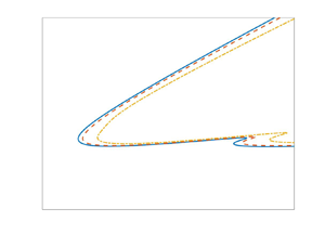
Neutral stability curves are replotted in figure 6 over a reduced $({Re},\alpha _r)$ range for both $\varphi =6$ and $\varphi =10$. The behaviour near the onset of the type I cross-flow instability and the type II Coriolis instability are shown in figure 6(a,c) and figure 6(b,d), respectively. The illustration further demonstrates the strong stabilising effect of time-periodic modulation on the cross-flow instability. However, the effect on the Coriolis instability is only noticeably different in the instance $\varphi =10$. Moreover, results suggest that the stabilising effect found for the cross-flow instability increases as the modulation amplitude $\epsilon$ increases.

Figure 6.

Same as figure 5 but over a reduced $({Re},\alpha _r)$ range, highlighting the behaviour near (a,c) the type I cross-flow instability and (b,d) the type II Coriolis instability. (a,b) The modulation frequency $\varphi =6$; (c,d) $\varphi =10$. The modulation amplitude $\epsilon =0$ (solid), $\epsilon = 0.1$ (dashed) and $\epsilon = 0.2$ (chain).

The above analysis was extended to encompass a range of modulation frequencies $\varphi$ and two modulation amplitudes: $\epsilon =0.1$ and $\epsilon =0.2$. Critical conditions for the onset of the stationary convective instability were then determined, with the critical Reynolds number ${Re}_c$ and azimuthal mode number $n_c$ plotted in figure 7. The horizontal chain lines depict the critical conditions obtained for the rotating disk without modulation, where ${Re}_c\approx 285.6$ and $n_c\approx 22$. The calculations for $\epsilon =0$ are consistent with those found in the earlier linear stability studies by Malik (Reference Malik1986) and Lingwood (Reference Lingwood1997), amongst many others. Table 3 presents numerical values for ${Re}_c$ and $n_c$, alongside the critical radial wavenumber $\alpha _c$, for several modulation $(\epsilon ,\varphi )$ settings. In all instances modelled, the most unstable disturbance corresponds to the cross-flow instability (given in bold); the type II Coriolis instability (given in brackets) emerges at significantly larger Reynolds numbers. Thus, the cross-flow instability is the most unstable form of disturbance and will ultimately be responsible for bringing about the early stages of laminar–turbulent transition on the modulated rotating disk. Furthermore, time-periodic modulation increases the Reynolds number for the onset of unstable behaviour, with a peak stabilising effect achieved for frequencies $\varphi \sim 8$. However, for modulation frequencies $\varphi >25$, the stabilising effect is negligible. Finally, the critical azimuthal mode number $n_c$ for linear instability is only marginally affected by modulating the disk rotation rate.

Figure 7.

(a) Critical Reynolds number ${Re}_c$ and (b) azimuthal mode number $n_c$ for the stationary type I cross-flow instability, as a function of the modulation frequency $\varphi$. The modulation amplitude $\epsilon = 0.1$ (solid line) and $\epsilon = 0.2$ (dashed). Solutions corresponding to the steady von Kármán flow are indicated by the horizontal chain lines.

Table 3.

Critical conditions for the onset of the stationary type I cross-flow instability (bold) and type II Coriolis instability (brackets). The cross-flow mode is the most dangerous in all instances modelled.

Optimum modulation frequencies $\varphi$ are presented in table 4 that establish the greatest level of stabilisation for both the type I cross-flow instability (bold) and type II Coriolis instability (italics). Numerical calculations indicate that different modulation frequencies are required to achieve the maximum stabilisation effect for the two forms of instability. While we might expect optimum $\varphi$ to be the same for both forms of instability, the differences reported in table 4 can be explained by noting that the two instabilities are brought about by very different mechanisms and so can be expected to react differently to the imposed modulation frequency. The cross-flow instability is inviscid in nature and is associated with an inflection point in the mean velocity profiles. On the other hand, the Coriolis instability is essentially viscous and is destabilised by the Coriolis forces present within the rotating disk boundary layer.

Table 4.

Optimum modulation frequencies $\varphi$ that establish the greatest level of stabilisation for the type I cross-flow instability (bold) and type II Coriolis instability (italics).

5.1. Formulation

In order to compute the energy balance across a full period of modulation, a Q-S formulation is adopted, whereby the homogeneous base flow (4.3) is frozen at each time-step. Thus, time $\tau$ is treated as a parameter, and the Floquet mode structure (4.11) is replaced by the simpler normal mode form

(5.1)\begin{equation} \boldsymbol{q}(r,\theta,z,\tau) = \tilde{\boldsymbol{q}}(z)\exp(\textrm{i}(\alpha r + n\theta-\omega\tau))+\textrm{c.c.}, \end{equation}

which is more commonly utilised in local stability studies on the steady rotating disk. The radial wavenumber and azimuthal mode number are again denoted by $\alpha$ and $n$, while the frequency $\omega =0$ for stationary disturbances. On substituting (5.1) into the governing perturbation (4.5), a single system of ordinary differential equations is established, given by the dispersion relationship

(5.2)\begin{equation} \mathcal{D}(\omega,\alpha;{Re},n,\tau)=0, \end{equation}

which is solved using the numerical methods outlined in § 4. By imposing the Q-S flow approximation, the stability problem is cast as a series of locally defined systems for a succession of different basic states at each phase during the modulation cycle.

The energy equation is formulated by multiplying the three linearised momentum equations by the respective velocity perturbation fields $\boldsymbol {u}=(u_r,u_{\theta },u_z)$, and summing together to give the following equation for the kinetic energy:

(5.3)\begin{align} &\left(\frac{\partial K}{\partial t} + U\frac{\partial K}{\partial r} + \frac{V}{r}\frac{\partial K}{\partial \theta} + W\frac{\partial K}{\partial z} \right) ={-}u_ru_z\frac{\partial U}{\partial z} - u_{\theta}u_z \frac{\partial V}{\partial z} - u_z^{2}\frac{\partial W}{\partial z} - u_r^{2}\frac{\partial U}{\partial r} - \frac{u_{\theta}^{2}U}{r} \nonumber\\ &\quad - \left(\frac{\partial}{\partial r}(u_rp) + \frac{1}{r}\frac{\partial }{\partial r}(u_{\theta}p) + \frac{\partial }{\partial z}(u_zp) + \frac{u_rp}{r}\right) + \left(\frac{\partial}{\partial x_i}(u_j\sigma_{ij}) - \sigma{ij}\frac{\partial u_j}{\partial x_i}\right), \end{align}

where $p$ represents the pressure perturbation field, $K = (u_r^{2} + u_{\theta }^{2} + w^{2})/2$, repeated suffices indicate summation and $\sigma _{ij}$ denotes the viscous stress terms

(5.4)\begin{equation} \sigma_{ij} = \frac{1}{{Re}}\left(\frac{\partial u_i}{\partial x_j} - \frac{\partial u_j}{\partial x_i}\right). \end{equation}

The $O(1/{Re}^{2})$ terms have been neglected for consistency with the Floquet analysis presented in § 4.

By averaging over a single azimuthal mode number $n$ and integrating across the boundary layer, azimuthal $\theta$-derivatives are removed from (5.3) to give

(5.5)\begin{align} &\int_{0}^{\infty}\left(\frac{\partial \bar{K}}{\partial t} + \underbrace{U\frac{\partial \bar{K}}{\partial r}}_{{(A)}} + \underbrace{\frac{\partial\left(\bar{u_rp}\right)}{\partial r}}_{{(B)}} - \underbrace{\frac{\partial}{\partial r}\left(\bar{u_{r}\sigma_{11}} +\bar{u_{\theta}\sigma_{12}} + \bar{u_z\sigma_{13}}\right)}_{{(C)}}\right) \,\textrm{d} z \nonumber\\ &\quad = \underbrace{\int_{0}^{\infty}\left(-\bar{u_ru_z}\frac{\partial U}{\partial z} - \bar{u_{\theta}u_z}\frac{\partial V}{\partial z} - \bar{u_z^{2}}\frac{\partial W}{\partial z} \right)\,\textrm{d} z}_{{(I)}} - \underbrace{\int_{0}^{\infty}\left(\bar{\sigma_{ij}\frac{\partial u_{j}}{\partial i}}\right) \,\textrm{d} z}_{{(II)}} \nonumber\\ &\qquad - \underbrace{\int_{0}^{\infty}\left(\frac{\bar{u_rp}}{r}\right) \,\textrm{d} z \!+\! (u_zp)_w}_{{(III)}} \!-\! \underbrace{(u_r\sigma_{31} \!+\! u_{\theta}\sigma_{32})_w}_{{(IV)}} - \underbrace{\int_{0}^{\infty}\left(W\frac{\partial \bar{K}}{\partial z}+\bar{u_r^{2}}\frac{\partial U}{\partial r}+\frac{\overline{u_{\theta}^{2}}U}{r}\right) \,\textrm{d} z}_{{(V)}}. \end{align}

The $w$ subscript in $(III)$ and $(IV)$ denotes a quantity evaluated at the disk wall, while overbars denote a period-averaged quantity. Velocity perturbation fields $\boldsymbol {u}$ are given as solutions of the dispersion relationship (5.2), while the pressure $p$ perturbation field is obtained by integrating the linearised $z$-momentum component of the Navier–Stokes equations to give the formula

(5.6)\begin{equation} p = \int_0^{\infty}\left(\frac{\partial u_z}{\partial t} + U\frac{\partial u_z}{\partial r} + \frac{1}{r{Re}}\frac{\partial (r \xi_{\theta})}{\partial r}\right) \,\textrm{d} z + Wu_z. \end{equation}

As described by Cooper and coauthors (Cooper & Carpenter Reference Cooper and Carpenter1997; Cooper et al. Reference Cooper, Harris, Garrett, Özkan and Thomas2015; Garrett et al. Reference Garrett, Cooper, Harris, Özkan, Segalini and Thomas2016), each term in (5.5) has a physical interpretation in terms of its contribution to the system energy. On the left-hand side, $(A)$ represents the average kinetic energy convected by the radial component of the base flow, $(B)$ the work done by the pressure perturbation field and $(C)$ the work done by the viscous stresses across some internal boundary in the fluid. For the subsequent analysis, the latter term $(C)$ is negligible. On the right-hand side, $(I)$ represents the Reynolds stress energy production, $(II)$ the viscous dissipation energy removal, $(III)$ the pressure work, $(IV)$ the contributions from work done on the wall by viscous stresses and $(V)$ the streamline curvature effects and the three-dimensionality of the mean flow.

Equation (5.5) is normalised by the integrated mechanical energy flux to give

(5.7)\begin{align} -2\alpha_i &={-}\frac{\partial K}{\partial t} + \underbrace{(P_1 + P_2 + P_3)}_{{(I)}} + \underbrace{D}_{{(II)}} + \underbrace{(PW_1 + PW_2)}_{{(III)}} \nonumber\\ &\quad + \underbrace{(S_1 + S_2 + S_3)}_{{(IV)}} + \underbrace{(G_1 + G_2 + G_3)}_{{(V)}}, \end{align}

where all terms, including the mechanical energy flux, are time-dependent. In particular, terms are time-periodic with a period $T$. Positive terms correspond to an energy production, while negative terms are matched to the removal of energy from the system. A disturbance is then amplified when the energy production exceeds the energy dissipation from the system, which corresponds to a negative radial growth rate $(\alpha _i < 0)$. All components of the energy balance equation (5.7) are then determined to identify those terms that are most affected by the time-periodic modulation.

It was shown by the Cooper group (Cooper & Carpenter Reference Cooper and Carpenter1997; Cooper et al. Reference Cooper, Harris, Garrett, Özkan and Thomas2015; Garrett et al. Reference Garrett, Cooper, Harris, Özkan, Segalini and Thomas2016) that the energy production due to the Reynolds stress $(P_2)$ and the viscous energy removal $(D)$ dominate (5.7) for the steady von Kármán flow, while $S_1, S_2, S_3$ and $PW_2$ are zero as a consequence of the boundary conditions. Furthermore, the remaining terms are negligible, with the exception of the geometric terms $G_1$ and $G_3$ for the type II Coriolis instability.

For the periodically modulated rotating disk flow (4.3), Q-S perturbations (5.1) and by extension the energy terms in (5.7), are computed over a full cycle $T$ of the time-periodic modulation. It is expected that quantities will vary across the period of modulation. Thus, to help draw comparisons with the solutions of the steady von Kármán flow, terms are averaged over one modulation period $T$, by computing the quantity

(5.8)\begin{equation} \bar{q}=\frac{1}{T}\int_0^{T}q \,\textrm{d} \tau. \end{equation}

For instance, $\bar {\alpha }_i$ denotes the time-averaged (T-A) radial growth rate over one modulation period.

In the following analysis, we compute the energy terms in (5.7) for two specific flow conditions that are matched to the type I cross-flow instability and the type II Coriolis instability. In the former instance the Reynolds number ${Re}=500$ and azimuthal mode number $n=32$, while in the latter case ${Re}$ is unchanged but $n=20$. The decision to focus on these modes, and in particular the $n=32$ cross-flow mode, was made as a consequence of earlier experimental observations that found the early stages of laminar–turbulent transition were dominated by azimuthal modes $n\in [28,32]$ (Gregory et al. Reference Gregory, Stuart and Walker1955; Kobayashi et al. Reference Kobayashi, Kohama and Takamadate1980; Jarre et al. Reference Jarre, Le Gal and Chauve1996). The effects of time-periodic modulation are then determined for modulation amplitudes $\epsilon =0.1$ and $0.2$, and frequencies $\varphi =6$ and $10$, and solutions compared against those results obtained for the steady von Kármán flow. These particular parameters were chosen as they correspond to a near optimal stabilisation of the cross-flow and Coriolis instabilities (recall figures 4–7). Although this only illustrates the effect of modulation on disturbance characteristics in a few specific instances, comparable behaviour was observed for other modulation settings and flow conditions.

5.2. Stationary type I cross-flow instability

The disturbance evolution matching the conditions given above for the stationary cross-flow instability are considered first. Figure 8(a) displays the variation of the radial wavenumber $\alpha$ in the complex $(\alpha _r,\alpha _i)$-plane, while figure 8(b) depicts the temporal evolution of the radial growth rate $\alpha _i$ as a function of time $\tau$. Solutions are plotted over one full period of time-periodic modulation, for the modulation amplitude $\epsilon =0.2$ and frequency $\varphi =10$. The radial growth rate $\alpha$ obtained for the steady von Kármán flow is indicated by the blue circular marker and solid blue line in the respective illustrations. Cross and square markers in figure 8(a) display the Q-S and T-A solutions of the modulated system, while the equivalent results in figure 8(b) are indicated by dashed and chain lines. The Q-S radial growth rate $\alpha _i$ fluctuates over the time interval shown. A minimum and maximum growth rate are realised about the respective $\tau /T=1/4$ and $\tau /T=3/4$ stages of the modulation cycle, which coincides with the unsteady part of the disk rotation rate (2.2) achieving a maximum and minimum, respectively (recall figure 2). The corresponding T-A radial growth rate $\bar {\alpha }_i$ indicates that a reduction in growth is achieved over a modulation period compared with the steady von Kármán flow. Hence, time-periodic modulation of the disk rotation rate is stabilising, which is to be expected given the earlier Floquet analysis.

Figure 8.

Evolution of the radial wavenumber $\alpha$, over one modulation period $T$, for the stationary type I cross-flow instability with the Reynolds number ${Re}=500$ and azimuthal mode number $n=32$. The modulation amplitude $\epsilon = 0.2$ and frequency $\varphi = 10$. (a) The $(\alpha _r,\alpha _i)$-plane, (b) $\alpha _i$ as a function of time $\tau /T$.

The corresponding radial wavenumber $\alpha$ obtained via Floquet linear stability theory is indicated by a star in figure 8(a), and coincides with the T-A wavenumber $\bar {\alpha }$ (square marker). Indeed, as shown in table 5, agreement between the Floquet and T-A wavenumbers is realised to at least two decimal places for the above parameter settings and in many other instances.

Table 5.

Radial growth rates obtained using Floquet theory and via a time-averaging of the Q-S solutions, for the stationary type I cross-flow instability with the Reynolds number ${Re}=500$ and azimuthal mode number $n=32$.

The evolution of the Reynolds stress energy production $(P_2)$ and viscous dissipation $(D)$ are plotted in figure 9, for modulation amplitudes $\epsilon =0.1$ and $0.2$, and the modulation frequency $\varphi =10$. Line types for the steady and modulated systems are the same as that given in figure 8. Quasi-steady solutions again fluctuate over the modulation cycle. The energy production $(P_2)$ displays behaviour qualitatively similar to the above description of the radial growth rate $\alpha _i$. A minima and maxima are observed about the quarter and three-quarter stages of the modulation cycle, which coincides with the time-periodic modulation attaining, respectively, a maximum and minimum (recall (2.2) and figure 2). The behaviour is reversed for the viscous dissipation, with maximum and minimum absolute values realised about $\tau /T=1/4$ and $\tau /T=3/4$, respectively. This particular feature of the energy balance is to be expected, as a reduction (increase) in the radial growth rate will establish a comparable drop (rise) and rise (drop) in the respective energy terms $P_2$ and $|D|$. Furthermore, as the modulation amplitude $\epsilon$ increases, there is a marginal increase in the maximum value of the energy production, while there is a significant decrease in the corresponding minimum value. On the other hand, the minimum absolute value of the viscous dissipation is relatively unchanged by increasing $\epsilon$, while there is a noticeable increase in the maximum absolute value. Since the energy terms $P_2$ and $D$ are, respectively, positive and negative, and are matched to an energy production and reduction, this behaviour would suggest that the stabilising effect induced by modulating the disk rotation rate will become more pronounced as the modulation amplitude $\epsilon$ increases. Finally, as $\epsilon$ increases, the T-A energy production $(\bar {P}_2)$ decreases and the T-A viscous dissipation $(\bar {D})$ attains a larger absolute value. Hence, the T-A calculations provide a further illustration of the stabilising effect brought about by the time-periodic modulation.

Figure 9.

Evolution of (a,b) the Reynolds stress energy production ($P_2$) and (c,d) the viscous dissipation $(D)$ across one full period $T$ of disk modulation. Modulation amplitudes $\epsilon$ are as given in the caption for the modulation frequency $\varphi =10$, for the stationary type I cross-flow instability with the Reynolds number ${Re}=500$ and azimuthal mode number $n=32$.

Figure 10 depicts the full energy balance of those terms given in (5.7), for the Reynolds number ${Re}=500$ and azimuthal mode number $n=32$. Results are plotted for the steady von Kármán flow and four time-periodically modulated systems that are based on the T-A calculations. Similar to the steady von Kármán flow, the Reynolds stress energy production and viscous dissipation energy removal are the most significant in all instances modelled. All remaining terms are again negligibly small. Furthermore, figure 10 displays behaviour comparable with the trends observed by Cooper & Carpenter (Reference Cooper and Carpenter1997) on wall compliance, and Garrett et al. (Reference Garrett, Cooper, Harris, Özkan, Segalini and Thomas2016) on surface roughness. Similar to these other flow control strategies, the stabilising effect brought about by time-periodic modulation corresponds to a reduction in $\bar {P}_2$ and an increase in $\bar {D}$. The illustration infers that the stabilising effect, induced by modulating the disk rotation rate, is enhanced for larger modulation amplitudes $\epsilon$ and frequencies $\varphi \sim 6$, which is consistent with the earlier Floquet analysis.

Figure 10.

Energy balance terms in (5.7) for the stationary type I cross-flow instability with the Reynolds number ${Re}=500$ and azimuthal mode number $n=32$. The solutions to the steady system (blue) are compared against four time-periodically modulated systems based on the T-A computations.

The T-A Reynolds stress energy production and viscous dissipation are plotted in figure 11 as a function of the azimuthal mode number $n$. Solutions correspond to the stationary type I cross-flow instability, with the Reynolds number ${Re}=500$ and modulation frequency $\varphi =10$. Results are plotted for three modulation amplitudes $\epsilon$, over the interval $30\leq n\leq 40$ that are the most unstable mode numbers for the given parameter settings. There is a marked reduction and growth in the respective energy terms $\bar {P}_2$ and $|\bar {D}|$, for all azimuthal mode numbers $n$ considered, which further emphasises the stabilising effect brought about by modulating the disk rotation rate.

Figure 11.

Variation in the T-A (a) Reynolds stress energy production ($\bar {P}_2$) and (b) the viscous dissipation $(\bar {D})$ with the azimuthal mode number $n$. Modulation amplitudes $\epsilon$ are as given in the caption for the modulation frequency $\varphi =10$ and the Reynolds number ${Re}=500$. Solutions correspond to the stationary type I cross-flow instability ($\bar {P}_2$ attains a maximum about $n=34.55$, $35.13$ and $36.33$, for $\epsilon =0$, $0.1$ and $0.2$, respectively).

5.3. Stationary type II Coriolis instability

The above analysis was extended to the type II Coriolis instability, where the Reynolds number ${Re}=500$ and azimuthal mode number $n=20$. Figure 12 depicts the corresponding full energy balance terms in (5.7), with the modulation parameter settings and colourbars the same as those given in figure 10. The T-A Reynolds stress energy production and viscous dissipation energy removal again dominate the energy (5.7), while the geometric terms $\bar {G}_1$ and $\bar {G}_3$ are also significant. Unlike the earlier studies on surface roughness (Cooper et al. Reference Cooper, Harris, Garrett, Özkan and Thomas2015; Garrett et al. Reference Garrett, Cooper, Harris, Özkan, Segalini and Thomas2016) that observed an increase in the energy production and a destabilisation of the Coriolis instability, time-periodic modulation establishes a small reduction in the magnitude of $\bar {P}_2$ and an increase in the absolute value of $\bar {D}$. This behaviour is identical to the effect of modulation on the stationary cross-flow instability, although the effect is less pronounced. Hence, modulating the disk rotation rate acts to stabilise both the stationary type I and II instabilities.

Figure 12.

Energy balance terms in (5.7) for the stationary type II Coriolis instability with the Reynolds number ${Re}=500$ and azimuthal mode number $n=20$. The solutions to the steady system (blue) are compared against four time-periodically modulated systems based on the T-A computations.