1. Introduction
Magnetic fields in astrophysical systems are thought to arise by amplification of a seed magnetic field by dynamo action. In this process, kinetic energy of motion is converted to magnetic energy. A generic dynamo is the small-scale or fluctuation dynamo that arises in any random or turbulent flow (Kazantsev Reference Kazantsev1968; Zeldovich, Ruzmaikin & Sokolov Reference Zeldovich, Ruzmaikin and Sokolov1983; Zeldovich, Ruzmaikin & Sokoloff Reference Zeldovich, Ruzmaikin and Sokoloff1990; Haugen, Brandenburg & Dobler Reference Haugen, Brandenburg and Dobler2004; Schekochihin et al.
Reference Schekochihin, Cowley, Taylor, Maron and McWilliams2004; Brandenburg & Subramanian Reference Brandenburg and Subramanian2005; Tobias, Cattaneo & Boldyrev Reference Tobias, Cattaneo, Boldyrev, Davidson, Kaneda and Sreenivasan2013; Brandenburg, Sokoloff & Subramanian Reference Brandenburg, Sokoloff and Subramanian2012; Bhat & Subramanian Reference Bhat and Subramanian2014). It is well known that when the magnetic Reynolds number
 $\mathit{Re}_{M}$
of such a flow is above a certain critical threshold
 $R_{\mathit{crit}}\sim 100$
, the magnetic field in the fluid is amplified rapidly on the eddy turnover time scales. This amplification is due to the random stretching by the velocity shear. Such shearing motions also lead to the magnetic field developing smaller and smaller spatial scales, until resistive diffusion becomes important to balance the growth. The field then becomes highly intermittent (Zeldovich et al.
Reference Zeldovich, Ruzmaikin and Sokoloff1990) with the kinematic eigenfunction having power peaked on the resistive scales (Kazantsev Reference Kazantsev1968). For a random flow driven on a (single) scale
 $l$
, the resistive scale is
 $l_{{\it\eta}}\sim l/\mathit{Re}_{M}^{1/2}$
, and for
 $\mathit{Re}_{M}\gg 1$
it is much smaller than the driving scale
 $l$
. Eventually the Lorentz force of the growing magnetic field provides a back-reaction to the dynamo action, leading to the saturation of magnetic field growth. The nature and spatial coherence of the field in the saturated state are of paramount importance to the observational signatures of this field in different astrophysical systems (Enßlin & Vogt Reference Enßlin and Vogt2006; Schekochihin & Cowley Reference Schekochihin and Cowley2006; Subramanian, Shukurov & Haugen Reference Subramanian, Shukurov and Haugen2006; Bhat & Subramanian Reference Bhat and Subramanian2013), but is however not well understood at present (Brandenburg & Subramanian Reference Brandenburg and Subramanian2005; Brandenburg et al.
Reference Brandenburg, Sokoloff and Subramanian2012; Tobias et al.
Reference Tobias, Cattaneo, Boldyrev, Davidson, Kaneda and Sreenivasan2013).
Indeed, there is considerable evidence for magnetic fields in several systems such as galaxy clusters (Clarke, Kronberg & Böhringer Reference Clarke, Kronberg and Böhringer2001; Clarke Reference Clarke2004) and in young galaxies (Bernet et al.
Reference Bernet, Miniati, Lilly, Kronberg and Dessauges-Zavadsky2008) from observations of Faraday rotation that these systems induce on background polarized sources. A possible origin of these fields is the fluctuation dynamo action. However, whether one can indeed reproduce the observed levels of Faraday rotation measure (FRM) depends on the spatial coherence of the fields produced by the fluctuation dynamo. As these systems typically have
 $\mathit{Re}_{M}\gg 1$
, the field needs to become much more coherent in the saturated state than it is at the kinematic stage for it to explain the observations (Bhat & Subramanian Reference Bhat and Subramanian2013).
The saturation of fluctuation dynamos has been studied via both direct numerical simulations(DNS)and some simple analyticalmodels.A simplemodel of Subramanian (Reference Subramanian1999) suggests that the dynamo can saturate by the Lorentz force driving the dynamo to its marginal state. In such a case, the magnetic field in the saturated state concentrates on scales
 $l_{c}\sim l/R_{\mathit{crit}}^{1/2}$
. As
 $R_{\mathit{crit}}\ll \mathit{Re}_{M}$
typically, this implies a much more coherent field in the saturated state of the dynamo than during the kinematic stage. Using DNS with large magnetic Prandtl numbers (
 $\mathit{Pr}_{M}=\mathit{Re}_{M}/\mathit{Re}\gg 1$
), but small fluid Reynolds numbers (
 $\mathit{Re}$
), Schekochihin et al. (Reference Schekochihin, Cowley, Taylor, Maron and McWilliams2004) argued that the fluctuation dynamo saturates with the magnetic field still concentrated on resistive scales. On the other hand, the simulations of Haugen, Brandenburg & Dobler (Reference Haugen, Brandenburg and Dobler2003), Haugen et al. (Reference Haugen, Brandenburg and Dobler2004) and Eyink et al. (Reference Eyink, Vishniac, Lalescu, Aluie, Kanov, Bürger, Burns, Meneveau and Szalay2013) with
 $\mathit{Pr}_{M}=1$
and a large
 $\mathit{Re}_{M}=\mathit{Re}\approx 10^{3}$
found that the magnetic integral scale is just a modest fraction of the velocity integral scale, and much larger than the resistive scale. One could then expect significant FRMs, as is also consistent with the theoretical expectation from Subramanian (Reference Subramanian1999) and the DNS results of Subramanian et al. (Reference Subramanian, Shukurov and Haugen2006), Cho & Ryu (Reference Cho and Ryu2009) and Bhat & Subramanian (Reference Bhat and Subramanian2013). The case when both
 $\mathit{Re}$
and
 $\mathit{Pr}_{M}$
are large, as in galactic and cluster plasmas, is of course not easy to simulate, and the saturation of the fluctuation dynamo could be quite different (Eyink Reference Eyink2011).
Note that DNS are limited by the
 $\mathit{Re}_{M}$
values that are achievable and still perhaps do not have a large enough
 $\mathit{Re}_{M}$
to determine the saturated state unambiguously. At the same time, the analytical models are still rather simplistic. In this context, one may wonder if there is any other independent and simple way of studying the generic saturation properties of fluctuation dynamos. We consider here map dynamos, which have been studied earlier to mimic kinematic fast dynamo action, and examine how such maps could saturate. Such map dynamos typically lead to a fractal structure of the field, where the field goes into smaller and smaller scales (Finn & Ott Reference Finn and Ott1988, Reference Finn and Ott1990; Childress & Gilbert Reference Childress and Gilbert1995). However, with the incorporation of a diffusive step in the map, they can lead to eigenfunctions that preserve their shape, and have the smallest scale determined by the resistivity (or the effective
 $\mathit{Re}_{M}$
). In the case of such map dynamos, one can reach much larger
 $\mathit{Re}_{M}$
than for the case of DNS. We then examine simple models of saturating the map dynamo and study how the spatial structure of the map eigenfunction changes from the kinematic to the saturated state. Our aim is then to gain insight into generic properties of the saturated states of the fluctuation dynamo itself.
In the next section we begin with the description of the standard stretch–twist–fold (STF) dynamo (Vaĭnshteĭn & Zel’dovich Reference Vaĭnshteĭn and Zel’dovich1972). The corresponding map model for the STF dynamo is outlined in § 3. Results from numerical simulation of the STF map dynamo for various
 $\mathit{Re}_{M}$
are given in § 4. The saturation of the STF map dynamos is taken up in § 5. The last section presents a discussion of the results and our conclusions.
2. Zeldovich’s stretch–twist–fold dynamo
To explain the possibility of the fast dynamos, i.e. growth of magnetic field even when resistivity tends to zero, Vaĭnshteĭn & Zel’dovich (Reference Vaĭnshteĭn and Zel’dovich1972) put forward a heuristic description referred to as the STF dynamo. The algorithm involves first stretching a closed flux tube to double its length (see, for example, figure 4.6 in Brandenburg & Subramanian Reference Brandenburg and Subramanian2005), preserving its volume (a characteristic of an incompressible flow). Assuming magnetic flux to be frozen in the fluid, the magnetic field doubles as the area of the cross-section goes down by a factor of 2. Next, the flux tube is twisted into a figure of eight and then folded so the direction of the magnetic field is the same in both sub-parts. Then both parts are merged together into one through small diffusive effects to occupy the same volume as the starting flux tube. A weak diffusion is thus required to make the process of merging irreversible by smoothing the region between the two flux tubes during joining without much loss in the flux or energy. (Note that diffusion is not essential for the process of amplification of magnetic field in the STF dynamo. Even in random flows where both constructive and destructive twisting and folding are possible, the probability of a constructive effect dominates and leads to field amplification (Molchanov, Ruzmaikin & Sokolov Reference Molchanov, Ruzmaikin and Sokolov1984; Zeldovich et al. Reference Zeldovich, Ruzmaikin and Sokoloff1990). However, without the diffusion, the map is in principle reversible, so that one can restore the previous state. This is not possible after the diffusive step. Of course, diffusion is also required to develop an eigenfunction of the STF dynamo.)
It may thus be more appropriate to refer to this process as the stretch–twist–fold–merge dynamo, although we continue with the standard terminology here.
Hence, the final flux tube becomes equivalent to the original single flux tube, but with a field that is double the initial field. It is important to mark the way the two parts are folded. If they are folded with fields pointing in opposite directions, it would lead to the cancellation of the field and can model the field reversals due to turbulence in the actual physical situation. For a constructive folding, with each step the flux and thus the magnetic field increases by a factor of 2; repeating the same process
 $n$
times, the magnetic field increases by a factor of
 $2^{n}$
. Thus the growth rate is
 ${\sim}T^{-1}\ln 2$
, where
 $T$
is the time for one STF step. The stretching can also be done in a non-uniform manner. Suppose the stretching is done non-uniformly, by stretching a fraction
 ${\it\beta}$
(where
 $0<{\it\beta}<1/2$
) of the circumference (
 $2{\rm\pi}R$
) by an amount
 $1/{\it\beta}$
and the remaining length
 $2{\rm\pi}{\it\alpha}R$
of the circumference by
 $1/{\it\alpha}$
(where
 ${\it\alpha}=1-{\it\beta}$
). Then this would give rise to the same growth rate in the magnetic field as before but in a non-uniform way. Repeated operation of the inhomogeneous STF process on a flux tube or on one that has developed reversals would lead to the magnetic field developing a fine-scale structure that can mimic the intermittent nature of the field generated by fluctuating dynamos.
3. Map models for Zeldovich’s stretch–twist–fold dynamos
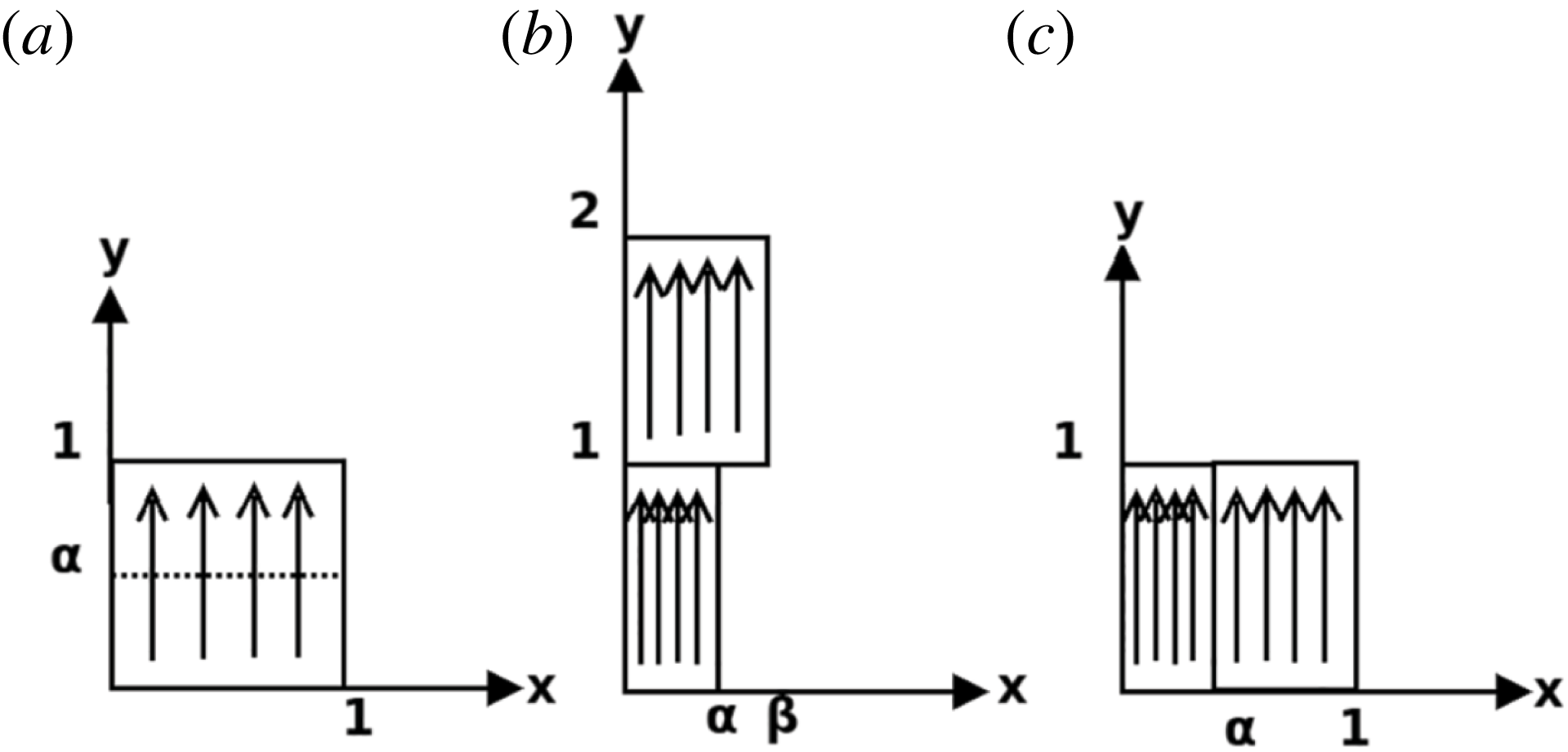
Finn & Ott (Reference Finn and Ott1988, Reference Finn and Ott1990) studied a map analogue of Zeldovich’s STF fast dynamo. Figure 1 represents the two-dimensional map that is used to model the dynamo. This map is an example of the generalized Baker’s map (Childress & Gilbert Reference Childress and Gilbert1995). We begin with a perfectly conducting two-dimensional square sheet in the
 $(x,y)$
plane, and a uniform upward (or
 $y$
) directed seed magnetic field of, say, unit strength. The magnetic field initially and at all times is independent of
 $y$
(analogous to being independent of the toroidal direction in a flux tube). Now, the lower part of the square
 $(0<y<{\it\alpha})$
is horizontally compressed by a factor of
 ${\it\alpha}$
and, to conserve the area, simultaneously stretched vertically by a factor of
 $1/{\it\alpha}$
. Similarly, the upper part
 $({\it\alpha}<y<1)$
is compressed by a factor of
 ${\it\beta}$
(along
 $x$
) and stretched by a factor of
 $1/{\it\beta}$
(along
 $y$
) where
 ${\it\beta}=1-{\it\alpha}$
. Then the two parts are separated, the magnetic field between the two parts is cut and the two pieces are rearranged to get back the original square. (This non-physical action allows one to describe an inherently three-dimensional physical process by a two-dimensional map; there cannot be any dynamo action in two-dimensional flows (Zeldovich et al.
Reference Zeldovich, Ruzmaikin and Sokolov1983).) As the flux is frozen in the region (
 ${\it\eta}\rightarrow 0$
), the field
 $B_{{\it\alpha}}$
through the
 ${\it\alpha}$
strip increases to
 $B/{\it\alpha}$
and the field
 $B_{{\it\beta}}$
through the
 ${\it\beta}$
strip increases by
 $B/{\it\beta}$
, where
 $B=1$
is the initial field. Then the total flux is
 $B{\it\alpha}+B{\it\beta}=2$
, and thus the flux through the entire square doubles. The average magnetic field also doubles within the square as compared to the initial field.
The two-dimensional Baker’s map as a model for the STF dynamo, but with non-uniform stretching.

The map that captures the above process is as follows:
 $$\begin{eqnarray}\displaystyle x_{n+1}\! & = & \displaystyle \!\left\{\begin{array}{@{}ll@{}}{\it\alpha}x_{n},\quad & \text{for}~y_{n}<{\it\alpha},\\ {\it\beta}x_{n}+{\it\alpha},\quad & \text{for}~y_{n}>{\it\alpha},\end{array}\right.\end{eqnarray}$$
 $$\begin{eqnarray}\displaystyle y_{n+1}\! & = & \displaystyle \!\left\{\begin{array}{@{}ll@{}}y_{n}/{\it\alpha},\quad & \text{for}~y_{n}<{\it\alpha},\\ (y_{n}-{\it\alpha})/{\it\beta},\quad & \text{for}~y_{n}>{\it\alpha}.\end{array}\right.\end{eqnarray}$$
 $x_{n}$
and
 $y_{n}$
take values in the interval
 $[0,1]$
. The corresponding amplification of the magnetic field in the region is given as
 $$\begin{eqnarray}B_{n+1}(x_{n+1})=\left\{\begin{array}{@{}ll@{}}B_{n}(x_{n})/{\it\alpha},\quad & \text{for}~x_{n}<{\it\alpha};\\ B_{n}(x_{n})/{\it\beta},\quad & \text{for}~x_{n}>{\it\alpha}.\end{array}\right.\end{eqnarray}$$
3.1. Amplification, cancellation and the four-strip map
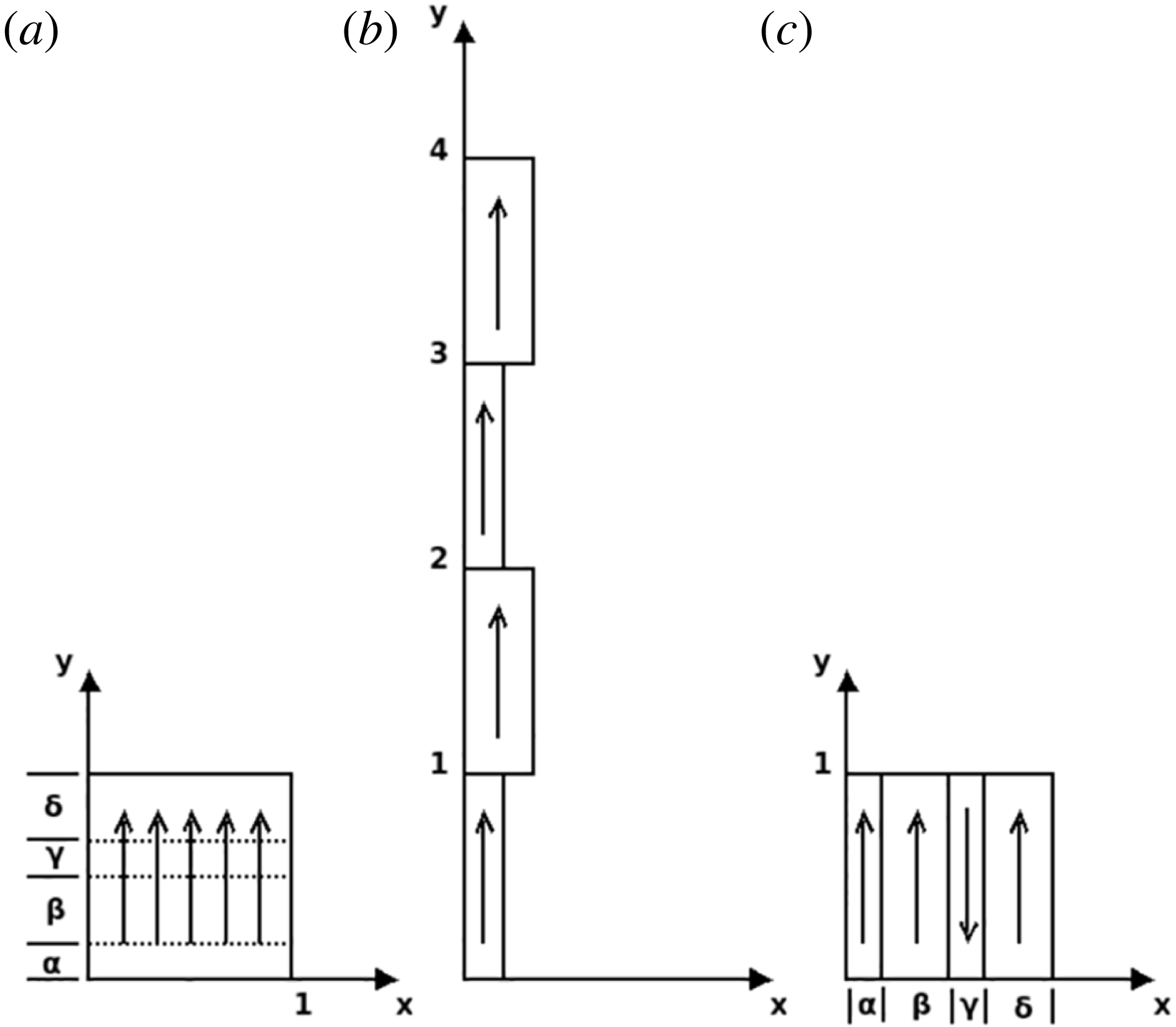
To include field reversals, which are an important part of the physical dynamo process leading to cancellation of magnetic fields, Finn & Ott (Reference Finn and Ott1988, Reference Finn and Ott1990) suggest a different model for STF dynamos. The flux tube in this case is stretched non-uniformly to four times its original circumference, twisted into four loops, and two of the loops are folded with the same orientation of magnetic field while the other two are folded with the opposite directions of fields, thus leading to a partial field cancellation. The corresponding map is shown in figure 2. The net field increase is the same as in the two-strip map – the field doubles with each step. As shown in figure 2, the analogous map would involve dividing the square into four strips and, while rearranging the strips, one of them is inverted and then placed to regain the initial square configuration. The analytical description of the four-strip map is given by
 $$\begin{eqnarray}\displaystyle x_{n+1}\! & = & \displaystyle \!\left\{\begin{array}{@{}ll@{}}{\it\alpha}x_{n},\quad & \text{for}~y_{n}<{\it\alpha},\\ {\it\beta}x_{n}+{\it\alpha},\quad & \text{for}~{\it\alpha}<y_{n}<({\it\alpha}+{\it\beta}),\\ {\it\gamma}(1-x_{n})+{\it\alpha}+{\it\beta},\quad & \text{for}~({\it\alpha}+{\it\beta})<y_{n}<({\it\alpha}+{\it\beta}+{\it\gamma}),\\ {\it\delta}x_{n}+{\it\alpha}+{\it\beta}+{\it\gamma},\quad & \text{for}~({\it\alpha}+{\it\beta}+{\it\gamma})<y_{n}<1,\end{array}\right.\end{eqnarray}$$
 $$\begin{eqnarray}\displaystyle y_{n+1}\! & = & \displaystyle \!\left\{\begin{array}{@{}ll@{}}y_{n}/{\it\alpha},\quad & \text{for}~y_{n}<{\it\alpha},\\ (y_{n}-{\it\alpha})/{\it\beta},\quad & \text{for}~{\it\alpha}<y_{n}<({\it\alpha}+{\it\beta}),\\ (({\it\alpha}+{\it\beta}+{\it\gamma})-y_{n})/{\it\gamma},\quad & \text{for}~({\it\alpha}+{\it\beta})<y_{n}<({\it\alpha}+{\it\beta}+{\it\gamma}),\\ (y_{n}-({\it\alpha}+{\it\beta}+{\it\gamma}))/{\it\delta},\quad & \text{for}~({\it\alpha}+{\it\beta}+{\it\gamma})<y_{n}<1.\end{array}\right.\end{eqnarray}$$
 $x_{n}$
and
 $y_{n}$
take values in the interval
 $[0,1]$
. The corresponding amplification of magnetic field with a flip of sign in the third strip is now given by
 $$\begin{eqnarray}B_{n+1}(x_{n+1})=\left\{\begin{array}{@{}ll@{}}B_{n}(x_{n})/{\it\alpha},\quad & \text{for}~y_{n}<{\it\alpha},\\ B_{n}(x_{n})/{\it\beta},\quad & \text{for}~{\it\alpha}<y_{n}<({\it\alpha}+{\it\beta}),\\ -B_{n}(x_{n})/{\it\gamma},\quad & \text{for}~({\it\alpha}+{\it\beta})<y_{n}<({\it\alpha}+{\it\beta}+{\it\gamma}),\\ B_{n}(x_{n})/{\it\delta},\quad & \text{for}~({\it\alpha}+{\it\beta}+{\it\gamma})<y_{n}<1.\end{array}\right.\end{eqnarray}$$
The two-dimensional four-strip Baker’s map as a model for the STF dynamo with cancellation of fields.

We will study both two-strip and four-strip maps in what follows.
3.2. Magnetic diffusion
As discussed above, it is important to include the smoothing effect of diffusion in the STF dynamo. We do this in the maps by convolving the evolved magnetic field after each step with a Gaussian. If
 $T$
is the time interval for each complete cycle of the STF map, the assumption is that for the time
 $T/2$
the diffusive term in the induction equation can be neglected, the flux is frozen and the field amplifies. For the remaining period,
 $T/2$
, the advection term vanishes and diffusion acts, with twice the normal diffusivity. The magnetic Reynolds number
 $\mathit{Re}_{M}$
is the measure of advection in comparison to diffusion and thus should be a parameter in the convolving function. The convolving Gaussian (also the Green’s function for diffusion) is therefore taken as (Finn & Ott Reference Finn and Ott1990)
 $$\begin{eqnarray}G(x,x^{\prime })=(\mathit{Re}_{M}/4{\rm\pi}T)^{1/2}\exp [-(x-x^{\prime })^{2}(\mathit{Re}_{M}/4T)].\end{eqnarray}$$
The width of the Gaussian (
 ${\it\sigma}=\sqrt{2T/\mathit{Re }_{M}}$
) is inversely proportional to
 $\sqrt{\mathit{Re }_{M}}$
and shows that the diffusion diminishes when
 $\mathit{Re}_{M}$
increases and vice versa. A single iteration involves applying the map to amplify the magnetic field and then convolving the evolved field with the above Gaussian.
4. Results: kinematic stage
We have coded the amplification of the magnetic field using the maps given in (5.3)–(3.6) and also included diffusion using the set of points in the unit square in the
 $(x,y)$
plane. The positions of the points are evolved using the map equations. The distribution of points in the interval
 $[0,1]$
is dynamic and the map automatically allocates more points to areas where the magnetic field has finer structure. This allows us to achieve higher
 $\mathit{Re}_{M}$
than the number of points that are used. We have generally adopted
 $300\times 300$
points for lower
 $\mathit{Re}_{M}$
runs, while for higher
 $\mathit{Re}_{M}$
we use
 $500\times 500$
points.
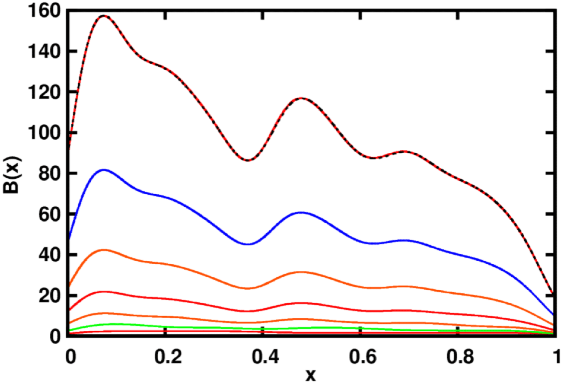
We first show in figure 3 the result of applying the two-strip map, excluding diffusion, to explore the kinematic evolution of the magnetic field starting from a unit seed field. Figure 3 shows the magnetic field
 $B(x)$
, as a function of position
 $x$
, after one, two, four and eight iterations. We have adopted
 ${\it\alpha}=0.4$
. It is clear from figure 3 that, as the number of iterations increases, the magnetic field grows but becomes more and more intermittent. Moreover, within a small spatial scale, the magnetic field varies significantly and develops a fractal structure (Finn & Ott Reference Finn and Ott1988, Reference Finn and Ott1990).
Magnetic field evolution in the two-strip map with
 ${\it\alpha}=0.4$
after (a) one, (b) two, (c) four and (d) eight iterations. The magnetic field strength
 $B(x)$
is given in units of the seed field. We see the amplification of the field strength and development of the intermittent structure of the field as the number of iterations increases.

4.1. Critical magnetic Reynolds number
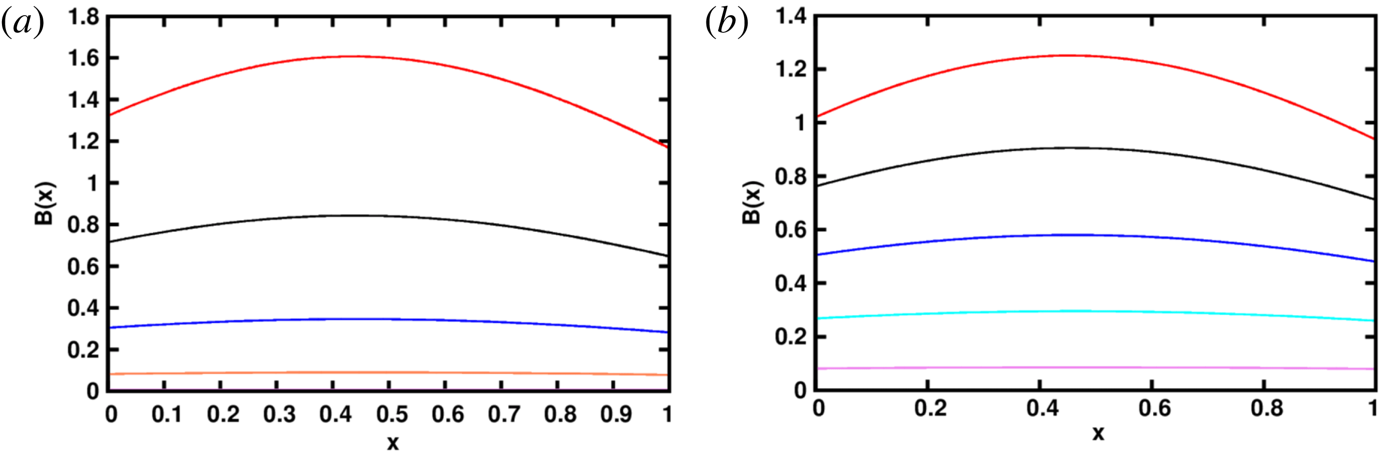
In the presence of diffusion, the amplification has to win over it for net amplification to occur. This introduces a critical
 $\mathit{Re}_{M}=R_{\mathit{crit}}$
, only above which does net amplification take place. We show in figure 4(a) that, starting with an initial seed field of 1,
 $B(x)$
is not amplified unless
 $\mathit{Re}_{M}>R_{\mathit{crit}}$
. The critical magnetic Reynolds number for the two-strip map is
 $R_{\mathit{crit}}\approx 4.35$
.
Plots of
 $B(x)$
for (a) the two-strip map and (b) the four-strip map, including diffusion, after eight iterations. In (a) the curves from bottom to top correspond to values of
 $\mathit{Re}_{M}=2$
, 3, 4, 5, respectively; while in (b) they correspond to
 $\mathit{Re}_{M}=1$
, 2, 3, 4, 5. The field is amplified for a critical magnetic Reynolds number
 $R_{\mathit{crit}}\gtrsim 4$
in both cases.

We have also incorporated diffusion into the four-strip map with cancellation adopting
 ${\it\alpha}={\it\delta}=7/16$
and
 ${\it\beta}={\it\gamma}=1/16$
. The results shown in figure 5(b) suggest a critical magnetic Reynolds number that is very close to that obtained for the two-strip map.
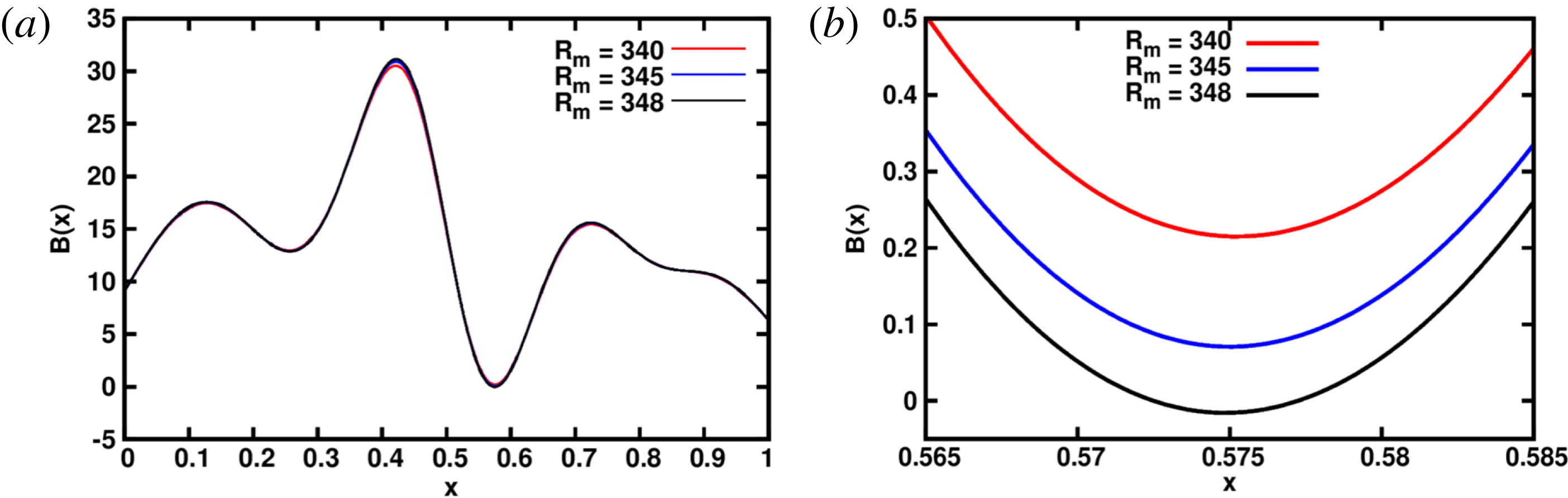
(a) Plot
 $B(x)$
for the four-strip map after four iterations, with the darkest curve corresponding to
 $\mathit{Re}_{M}=348$
. (b) A magnified version. It can be seen that
 $B(x)$
becomes negative first for
 $\mathit{Re}_{M}\sim 348$
, depending on the stretching parameters. Here we have adopted
 ${\it\alpha}={\it\delta}=7/16$
and
 ${\it\beta}={\it\gamma}=1/16$
.

It is interesting to note that, in the four-strip map, where the magnetic fields of both polarities are amplified, there is no field with negative polarity in the solution till a large enough
 $\mathit{Re}_{M}$
is reached. This critical
 $\mathit{Re}_{M}$
of course depends on the stretching parameters, in particular the value of
 ${\it\gamma}$
, which determines the degree of amplification of the negative field. As shown in figure 5, the field in the region has negative polarity solutions only for
 $\mathit{Re}_{M}\gtrsim 348$
for
 ${\it\alpha}={\it\delta}=7/16$
and
 ${\it\beta}={\it\gamma}=1/16$
.
4.2. Eigenfunctions of the map dynamo
After a few iterations, the function
 $B(x)$
representing the variation of the magnetic field along
 $x$
settles to an eigenfunction of a specific shape and
 $B(x)$
from future iterations can be matched to it by scaling. This can be seen in figure 6 for the two-strip map. For example,
 $B(x)$
after the seventh iteration can be scaled back in amplitude to
 $B(x)$
after the sixth iteration. Thus
 $B(x)$
tends to an eigenfunction of the map with diffusion included (which represents the STF dynamo). The eigenfunction of the two-strip map depends of course on
 $\mathit{Re}_{M}$
.
Plot of
 $B(x)$
for the two-strip map for one to seven iterations (from bottom to top), adopting
 ${\it\alpha}=0.4$
and
 $\mathit{Re}_{M}=1000$
. After the seventh iteration
 $B(x)$
is just a scaled version of
 $B(x)$
after the sixth one, illustrating the development of the map eigenfunction.

This is clear from figure 7: the eigenfunction of the magnetic field develops a finer and finer structure with increasing
 $\mathit{Re}_{M}$
(from
 $10^{2}$
to
 $10^{5}$
). The eigenfunctions shown in figure 7 for different values of
 $\mathit{Re}_{M}$
match those in figure 6 of Finn & Ott (Reference Finn and Ott1990) for the same
 ${\it\alpha}=0.4$
. The eigenfunctions for the four-strip map with
 $\mathit{Re}_{M}$
ranging from
 $10^{2}$
to
 $10^{5}$
are shown in figure 8. Besides showing features similar to the two-strip maps, the eigenfunctions of the four-strip map have fine-scale reversals of magnetic field. These could be thought of as an analogue of the field reversals seen in the DNS of fluctuation dynamos (Schekochihin et al.
Reference Schekochihin, Cowley, Taylor, Maron and McWilliams2004; Brandenburg & Subramanian Reference Brandenburg and Subramanian2005).
Eigenfunctions for the two-strip map with
 ${\it\alpha}=0.4$
and for (a)
 $\mathit{Re}_{M}=100$
, (b) 1000, (c)
 $10^{4}$
and (d)
 $10^{5}$
.

Eigenfunctions for the four-strip map for (a)
 $\mathit{Re}_{M}=100$
, (b) 1000, (d)
 $10^{4}$
and (d)
 $10^{5}$
. We have adopted
 ${\it\alpha}={\it\delta}=7/16$
and
 ${\it\beta}={\it\gamma}=1/16$
.

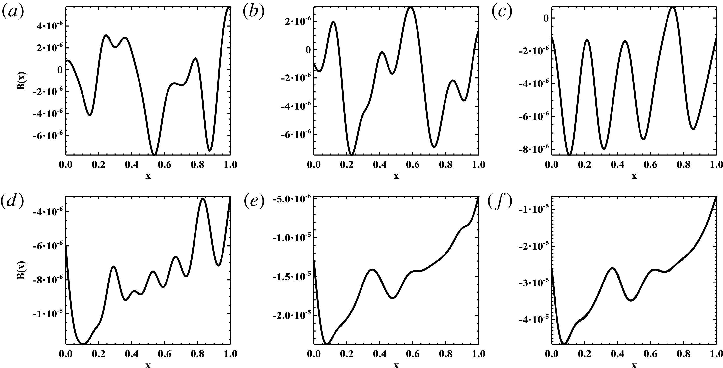
An interesting case is when we use a random initial seed field, instead of a uniform one. In figure 9, we show the evolution of such a run, from (a) to (f). It can be seen that, as the run progresses, the initial random field with both positive and negative values changes to an eigenfunction that is entirely negatively valued. This is clear on noting that the zero on the ordinate axis rapidly moves up, showing that
 $B(x)$
becomes more and more negative as it latches on to the eigenfunction. The
 $B(x)$
in figure 9( f) is the same eigenfunction as in the
 $Rm=1000$
case in figure 7, but with a negative amplitude. It could as well have become entirely positively valued depending on the initial seed field. This example also illustrates the fact that the eigenfunction of the map is realized independently of the initial conditions.
Evolution of
 $B(x)$
starting from a random initial seed field, for
 $\mathit{Re}_{M}=1000$
. The iteration number increases from (a) to ( f). The
 $B(x)$
plot in ( f) is the same eigenfunction as the
 $Rm=1000$
case in figure 7, but with a negative amplitude.

4.3. Fourier analysis of the magnetic field
We can also calculate the Fourier series for
 $B(x)$
to study the distribution of the magnetic power on different scales. The Fourier series is given by
 $$\begin{eqnarray}\tilde{B}(k)=\int _{0}^{1}B(x)\,\text{e}^{-2{\rm\pi}\text{i}xk}\,\text{d}x,\end{eqnarray}$$
where
 $k$
is wavenumber conjugate to
 $x$
. Then the magnetic power spectrum can be defined as
 $M(k)=|\tilde{B}(k)\tilde{B}^{\ast }(k)|/2$
.
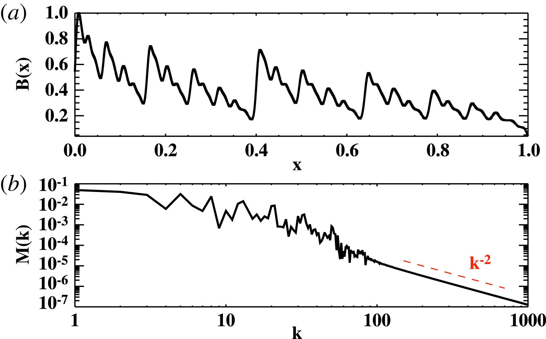
In figure 10, we show
 $M(k)$
corresponding to the eigenfunction
 $B(x)$
resulting from the two-strip map dynamo with
 $\mathit{Re}_{M}=10^{5}$
. The log–log plot does not show
 $M(k)$
for
 $k=0$
, which holds a significant amount of total power. However, in the given context, the
 $k=0$
component is just an overall constant factor in the eigenfunction and we would instead like to focus on the distribution of the power on smaller scales. We find that
 $M(k)$
is non-smooth and can vary sharply within adjacent values of
 $k$
. This is due to the fractal nature of the eigenfunction,
 $B(x)$
. For fractal functions, several intermediate coefficients in their Fourier series are expected to be zero (Korner Reference Korner1988).
(a) The eigenfunction
 $B(x)$
for a two-strip map dynamo for
 $\mathit{Re}_{M}=10^{6}$
. (b) The corresponding power spectrum
 $M(k)$
.

Note that
 $M(k)$
at large
 $k$
follows as
 $1/k^{2}$
. This is because, at large
 $k$
, the sines and cosines in (4.1) would sample a nearly constant part of
 $B(x)$
(or a ramp function in this case), and the Fourier transform of the ramp function is
 $\propto 1/k^{2}$
. In figures 11, 13 and 17, we show
 $M(k)$
for both two-strip and four-strip cases for different
 $\mathit{Re}_{M}$
in the kinematic stage and compare it to the saturated one. We will say more about these figures below in the following section.
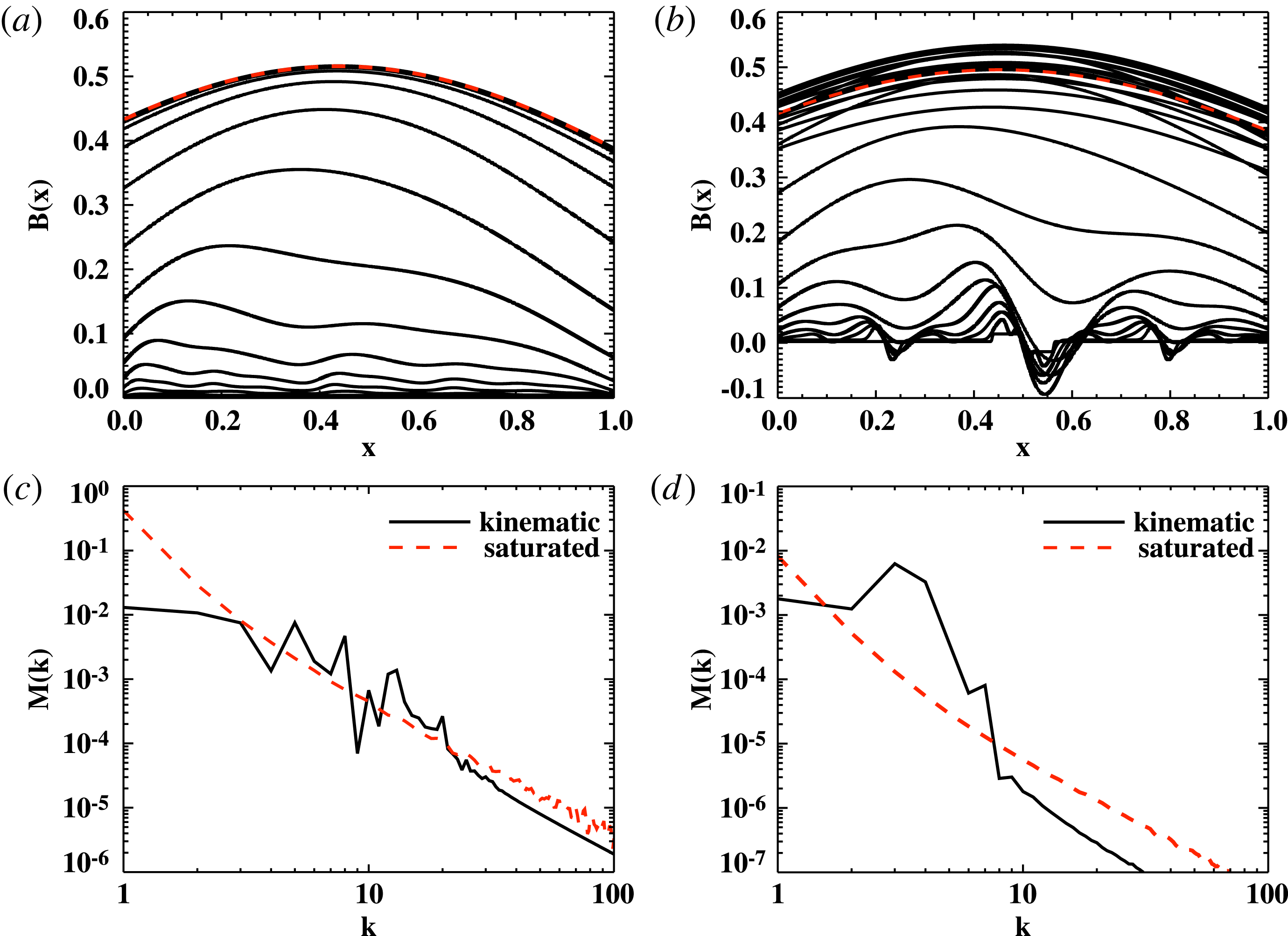
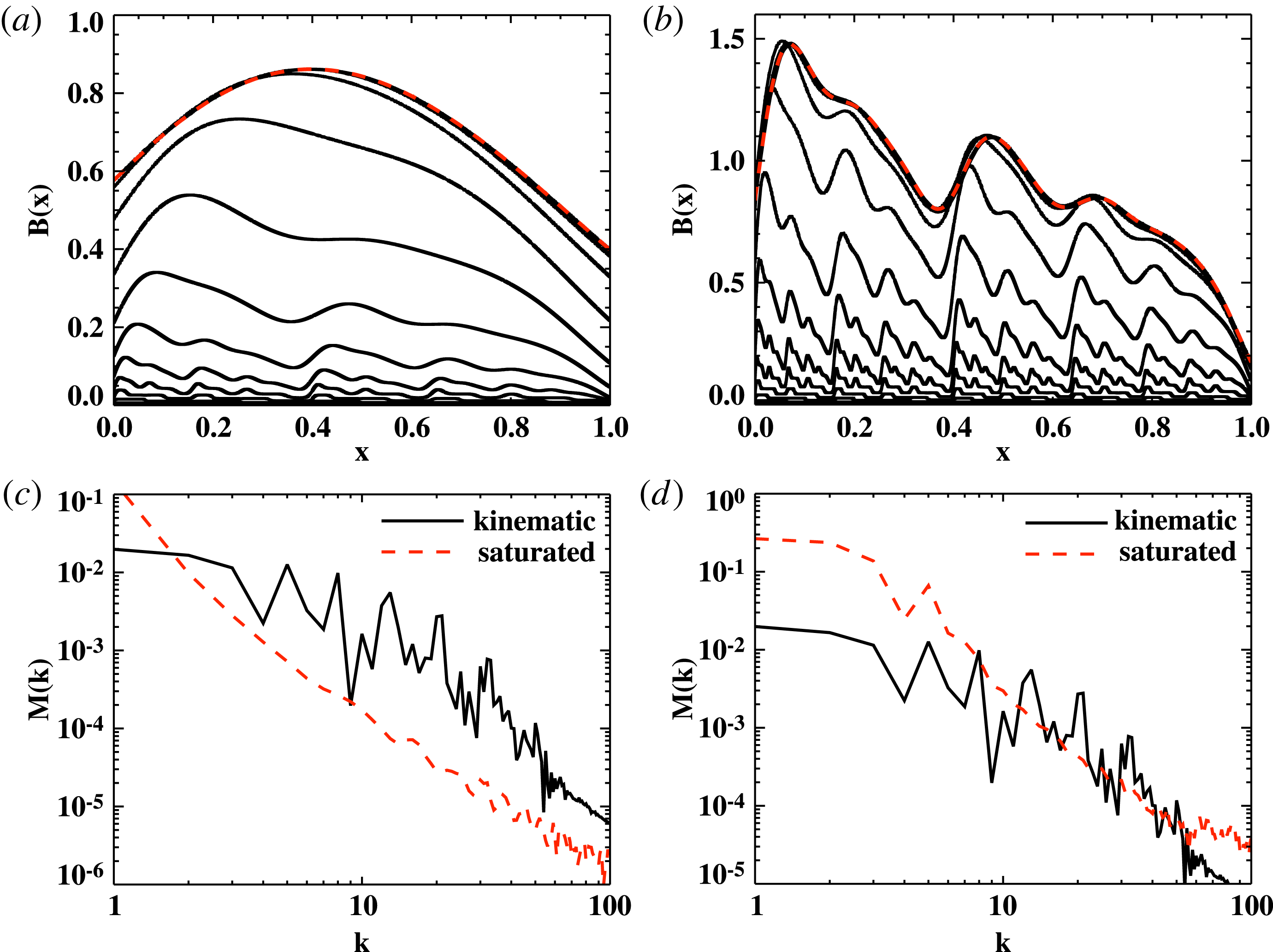
The nonlinear evolution of
 $B(x)$
, due to saturation by increasing resistivity. (a) Two-strip map evolution adopting
 ${\it\alpha}=0.4$
and initial
 $\mathit{Re}_{M}=10^{4}$
. (b) Four-strip map evolution with
 ${\it\alpha}={\it\delta}=7/16$
,
 ${\it\beta}={\it\gamma}=1/16$
and initial
 $\mathit{Re}_{M}=10^{6}$
. We see that the eigenfunction in both cases is driven to that of the marginal eigenfunction corresponding to
 $\mathit{Re}_{M}=R_{\mathit{crit}}$
on saturation. (c,d) The magnetic power spectrum,
 $M(k)$
, for the two cases, respectively. The bold black line shows
 $M(k)$
in kinematic regime and the red dashed line is the saturated case.

5. Saturation of stretch–twist–fold map dynamos
Saturation of dynamos can occur in several different ways. Possibilities include the renormalization and increase of the effective resistivity due to Lorentz forces (Subramanian Reference Subramanian1999) or the decreased stretching efficiency (Schekochihin et al.
Reference Schekochihin, Cowley, Taylor, Maron and McWilliams2004). We model these in simple ways below to study the saturation of the map dynamos. We will now set the absolute value of the saturated magnetic field strength to be of order unity, and therefore start with an initial seed field of
 $10^{-4}$
.
5.1. Saturation by decreasing
 $\mathit{Re}_{M}$

As one possibility, consider saturating the dynamo by a nonlinear increase of the effective resistivity as in the ambipolar drift model of Subramanian (Reference Subramanian1999). In this model, as the magnetic field grows and Lorentz forces become important, the effective resistivity becomes
 ${\it\eta}={\it\eta}_{0}+{\it\tau}B_{rms}^{2}/4{\rm\pi}{\it\rho}$
. Here
 ${\it\eta}_{0}$
is the microscopic resistivity,
 ${\it\tau}$
is a response time,
 ${\it\rho}$
is the fluid density and
 $B_{rms}$
is the root-mean-square (r.m.s.) value of
 $|\boldsymbol{B}|$
. Multiplying and dividing the second term in
 ${\it\eta}$
by
 $v^{2}$
, where
 $v$
is the r.m.s. turbulent velocity, we can rewrite this as
 ${\it\eta}={\it\eta}_{0}(1+R_{M0}B_{rms}^{2}/B_{eq}^{2})$
, where
 $R_{M0}=v^{2}{\it\tau}/{\it\eta}_{0}$
and
 $B_{eq}^{2}=4{\rm\pi}{\it\rho}v^{2}$
. Thus
 ${\it\eta}_{0}/{\it\eta}=\mathit{Re}_{M}/R_{M0}=(1+R_{M0}B_{rms}^{2}/B_{eq}^{2})^{-1}$
. We adopt such a picture for the map dynamo as well and model the nonlinear effect of the growing field by varying
 $\mathit{Re}_{M}$
at every iteration as
 $$\begin{eqnarray}\mathit{Re}_{M}=\frac{R_{M0}}{1+R_{M0}B_{rms}^{2}}.\end{eqnarray}$$
Again,
 $R_{M0}$
is the initial value of
 $\mathit{Re}_{M}$
for the map and
 $B_{rms}^{2}$
is now the average value of
 $B^{2}(x)$
at any iteration (or time), taken to be normalized to the equipartition value.
This form models the possible increase of the renormalized resistivity due to Lorentz forces.
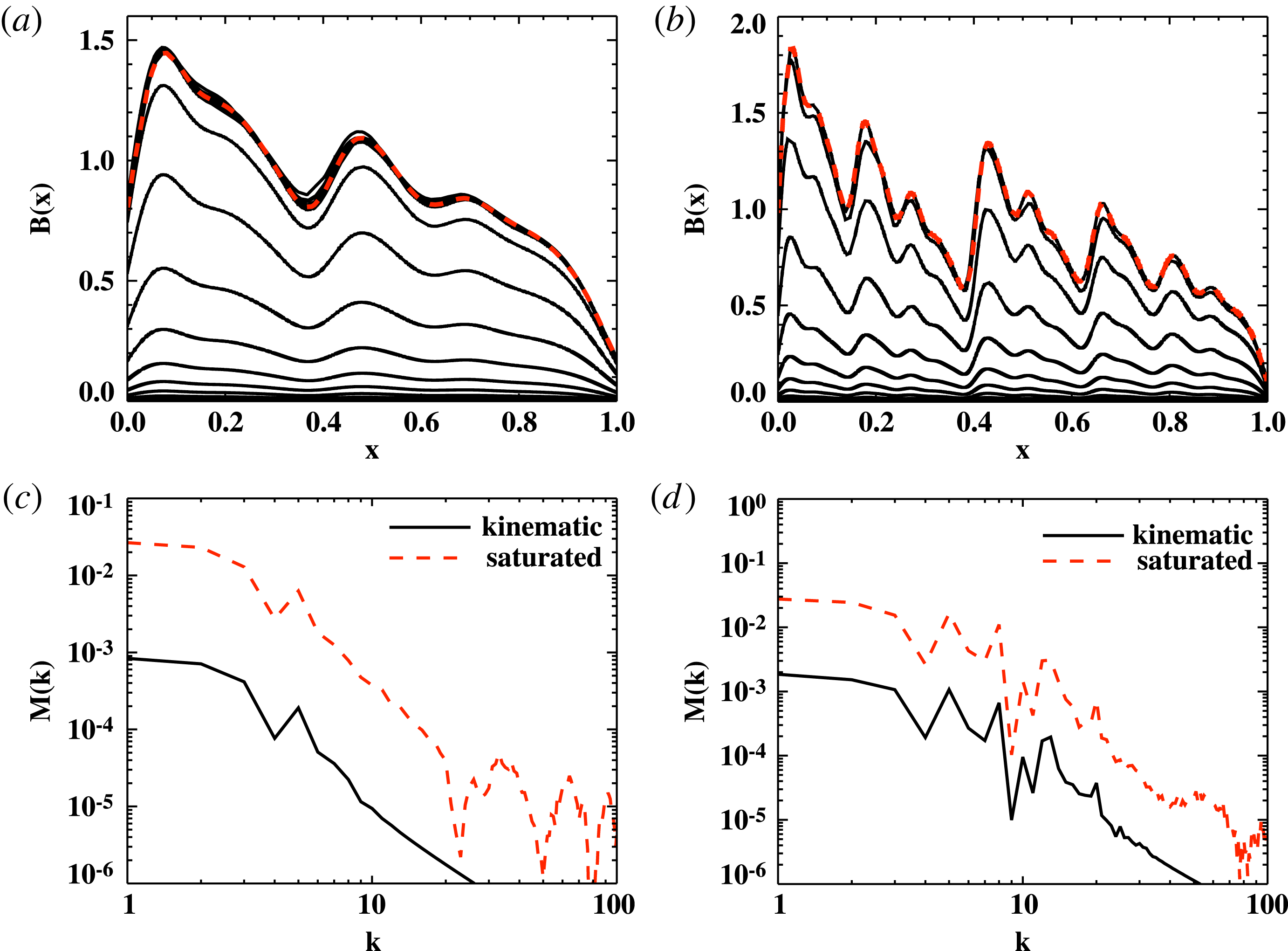
The time evolution of
 $B(x)$
is shown in figure 11(a,b) for two-strip,
 $R_{M0}=10^{4}$
, and four-strip,
 $R_{M0}=10^{6}$
, respectively. The evolution of the corresponding
 $B_{rms}$
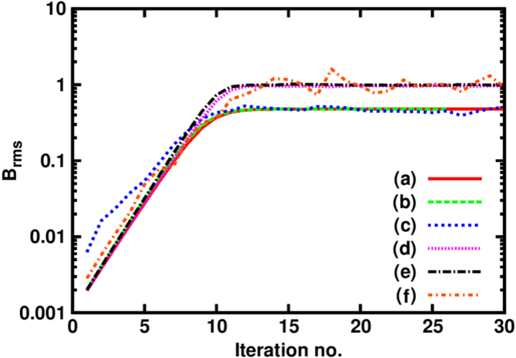
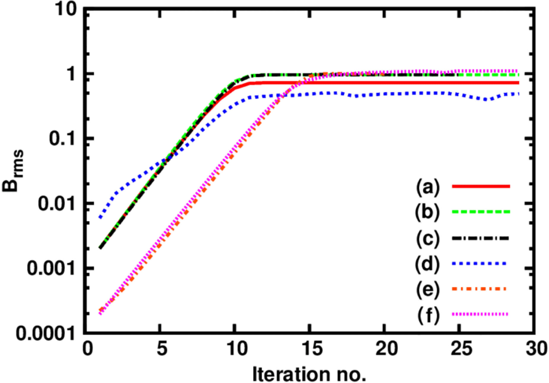
is shown in figure 12 as cases (a) and (c), respectively. We see from figure 12 that
 $B_{rms}$
indeed saturates after about 7–10 iterations, to a value of order unity. Moreover, on comparing figure 11(a,c) with figure 4(a) and figure 11(b,d) with figure 4(b), it is clear that the function
 $B(x)$
representing the saturated state is of the same form as
 $B(x)$
for the critical
 $\mathit{Re}_{M}~({\sim}4.35)$
. Further, in the saturated stage, the
 $\mathit{Re}_{M}$
given by (5.1) also settles to
 $R_{\mathit{sat}}=R_{\mathit{crit}}\sim 4$
, using
 $B_{rms}\sim 0.5$
and
 $R_{M0}=1000$
.
Comparison of
 $B_{rms}$
for various cases: (a) two-strip map with
 $\mathit{Re}_{M}=1000$
, saturation by decreasing
 $\mathit{Re}_{M}$
; (b) two-strip map with
 $\mathit{Re}_{M}=10^{4}$
, saturation by decreasing
 $\mathit{Re}_{M}$
; (c) four-strip map with
 $\mathit{Re}_{M}=10^{6}$
, saturation by decreasing
 $\mathit{Re}_{M}$
; (d) two-strip map with
 $\mathit{Re}_{M}=1000$
, saturation by decreasing stretching; (e) two-strip map with
 $\mathit{Re}_{M}=10^{4}$
, saturation by decreasing stretching; and (f) four-strip map with
 $\mathit{Re}_{M}=1000$
, saturation by decreasing stretching.

The nonlinear evolution of
 $B(x)$
of the two-strip map, due to saturation by reduced stretching, adopting initial
 ${\it\alpha}_{0}=0.4$
and (a)
 $\mathit{Re}_{M}=1000$
and (b)
 $\mathit{Re}_{M}=10^{4}$
. The red dashed line shows
 $B(x)$
in saturated state. (c,d) The magnetic power spectrum,
 $M(k)$
, for the two cases, respectively. The bold black line shows
 $M(k)$
in kinematic regime and the red dashed line is the saturated case.

In figure 11, we also show the corresponding magnetic power spectrum,
 $M(k)$
, where the solid black curve is from the kinematic stage and the red dashed line is for the saturated field. It can be seen that the kinematic field exhibits peaks on smaller scales, around
 $k\sim 5{-}20$
in the two-strip case and
 $k\sim 3{-}10$
in the four-strip case. The peaks seen on smaller scales (or larger
 $k$
) in the kinematic stage seem to be smoothed out by saturation with an increase in the power in
 $k\sim 1{-}2$
. Note that in both stages, however, the maximum power is in the
 $k=0$
constant component, which does not appear in such a log–log plot. Thus in the case where saturation is obtained by renormalization of
 $\mathit{Re}_{M}$
, we find that the saturated state has the same spatial structure as the marginal state of the kinematic map dynamo. Such a result is similar to the saturation behaviour obtained in Subramanian (Reference Subramanian1999) and perhaps in the simulations of Haugen et al. (Reference Haugen, Brandenburg and Dobler2004) for the
 $\mathit{Pr}_{M}=1$
fluctuation dynamo.
5.2. Saturation by decreasing stretching
5.2.1. Without changing the map
As the magnetic field strength increases, the effect of the Lorentz force would be to make it more difficult to amplify the field by stretching. Therefore, another way to achieve saturation in the maps would be to decrease the field amplification factor
 $\propto 1/{\it\alpha}$
as a function of
 $B_{rms}$
. We model this effect by multiplying
 ${\it\alpha}$
,
 ${\it\beta}$
in (5.5) for the two-strip map and
 ${\it\alpha}$
,
 ${\it\beta}$
,
 ${\it\gamma}$
,
 ${\it\delta}$
in (3.6) for the four-strip map by
 $(1+B_{rms}^{2})$
. For example, we adopt
 $$\begin{eqnarray}{\it\alpha}={\it\alpha}_{0}(1+B_{rms}^{2}),\end{eqnarray}$$
where
 ${\it\alpha}_{0}$
is the initial value of
 ${\it\alpha}$
. Note that, to begin with, we still leave the mapping of
 $(x_{n},y_{n})\rightarrow (x_{n+1},y_{n+1})$
described by (3.1), (3.2), (3.4) and (3.5) as before, described by the initial
 ${\it\alpha}_{0}$
,
 ${\it\beta}_{0}$
,
 ${\it\gamma}_{0}$
and
 ${\it\delta}_{0}$
. Thus the unit square in the
 $x{-}y$
plane is still mapped to the unit square, but the amplification by stretching becomes progressively inefficient as
 $B_{rms}$
grows.
Note that, as one reduces stretching by a factor of
 $f_{0}=1/(1+B_{rms}^{2})$
and applies the STF map to a flux tube, its final radius
 $R$
would decrease by
 $f_{0}$
while its cross-sectional area
 $A$
would increase by
 $1/f_{0}$
. In principle, the physical dimensions of the unit square that we use to represent the flux tube would then change accordingly and it will become a rectangle with its
 $y$
dimension (analogous to the length of the flux tube) reduced by
 $f_{0}$
and its
 $x$
dimension (analogous to the cross-sectional area of the flux tube) increased by
 $1/f_{0}$
. However, we are thinking of the unit square used in the map as representing the normalized flux tube radius and the normalized cross-sectional area. It is in this sense that the unit square is mapped onto itself, even though the degree of stretching is reducing with the growth of the field. We also now do not change the value of
 $\mathit{Re}_{M}$
during the diffusive step.
Theresult ofsuch reducedstretchingfor thetwo-strip mapis shownin figure 13(a,b) for
 $\mathit{Re}_{M}=1000$
and
 $\mathit{Re}_{M}=10^{4}$
, respectively. The corresponding
 $B_{rms}$
, whose evolution is shown in figure 12 as cases (d) and (e), saturates after about 10 iterations. It is clear from comparing figure 13 with figure 7 that the distribution
 $B(x)$
representing the saturated state in this case retains the complex structure of the growing kinematic eigenfunction and is quite different from the case of saturation by increased resistivity. It is thus not the marginal eigenfunction. In figure 13, we also show the magnetic power spectrum
 $M(k)$
in (c,d). Here again we see peaks on small scales, at
 $k\sim 6$
for
 $\mathit{Re}_{M}=1000$
and
 $k\sim 4{-}20$
for
 $\mathit{Re}_{M}=10^{4}$
. The saturated spectrum here matches with the one in the kinematic stage. This saturation behaviour is similar to what is argued by Schekochihin et al. (Reference Schekochihin, Cowley, Taylor, Maron and McWilliams2004) for the fluctuation dynamo with large
 $\mathit{Pr}_{M}$
, that the field in the saturated state appears to be qualitatively similar to the growing field in the kinematic stage.
We have also employed a similar scheme for the four-strip map with
 $\mathit{Re}_{M}=1000$
. The results shown in figure 14 indicate a very different saturation behaviour. Now, the saturated eigenfunction
 $B(x)$
oscillates with time, although its form is similar to the kinematic eigenfunction. Also
 $B_{rms}$
oscillates about a steady value around unity, as can be seen in figure 12 (case (f)). This seems to indicate that, if reversals are present, the saturated eigenfunction may never settle to a unique form.
Same as figure 13 but now for the four-strip map adopting an initial
 ${\it\alpha}_{0}={\it\delta}_{0}=7/16,{\it\beta}_{0}={\it\gamma}_{0}=1/16$
and
 $\mathit{Re}_{M}=1000$
. The eigenfunction on saturation oscillates with a structure similar to the kinematic eigenfunction. The shape of the kinematic eigenfunction is shown in dashed (red) line.

5.2.2. Changing the map
On reduced stretching, as explained earlier, the physical dimensions of a unit square map will change to become a rectangle. In the previous subsection, such a changed map is renormalized to a unit square before the diffusion is carried out, thus effectively not changing the map. We now explore the consequences of renormalizing the map to a unit square only after the diffusion step, before we carry out further STF mapping. This renormalization process is to ensure that the next STF mapping can be done, as before, on a unit square. Such a modified mapping for the two-strip case can be given as:
 $$\begin{eqnarray}\displaystyle x_{n+1}\! & = & \displaystyle \!\left\{\begin{array}{@{}ll@{}}{\it\alpha}_{1}x_{n},\quad & \text{for}~y_{n}<{\it\alpha},\\ {\it\beta}_{1}x_{n}+{\it\alpha}_{1},\quad & \text{for}~y_{n}>{\it\alpha},\end{array}\right.\end{eqnarray}$$
 $$\begin{eqnarray}\displaystyle y_{n+1}\! & = & \displaystyle \!\left\{\begin{array}{@{}ll@{}}y_{n}/{\it\alpha}_{1},\quad & \text{for}~y_{n}<{\it\alpha},\\ (y_{n}-{\it\alpha})/{\it\beta}_{1},\quad & \text{for}~y_{n}>{\it\alpha}.\end{array}\right.\end{eqnarray}$$
 $$\begin{eqnarray}B_{n+1}(x_{n+1})=\left\{\begin{array}{@{}ll@{}}B_{n}(x_{n})/{\it\alpha}_{2},\quad & \text{for}~x_{n}<{\it\alpha}_{1},\\ B_{n}(x_{n})/{\it\beta}_{2},\quad & \text{for}~x_{n}>{\it\alpha}_{1},\end{array}\right.\end{eqnarray}$$
where, initially, both
 ${\it\alpha}_{1}$
and
 ${\it\alpha}_{2}$
are
 ${\it\alpha}_{0}$
. After the diffusion step, once we evaluate the current
 $B_{rms}$
, we estimate
 ${\it\alpha}_{1}^{n}={\it\alpha}_{1}^{n-1}(1+B_{rms}^{2})$
, where
 ${\it\alpha}_{1}^{n}$
is the
 ${\it\alpha}_{1}$
of the
 $n$
th iteration and
 ${\it\alpha}_{2}={\it\alpha}_{0}(1+B_{rms}^{2})$
.
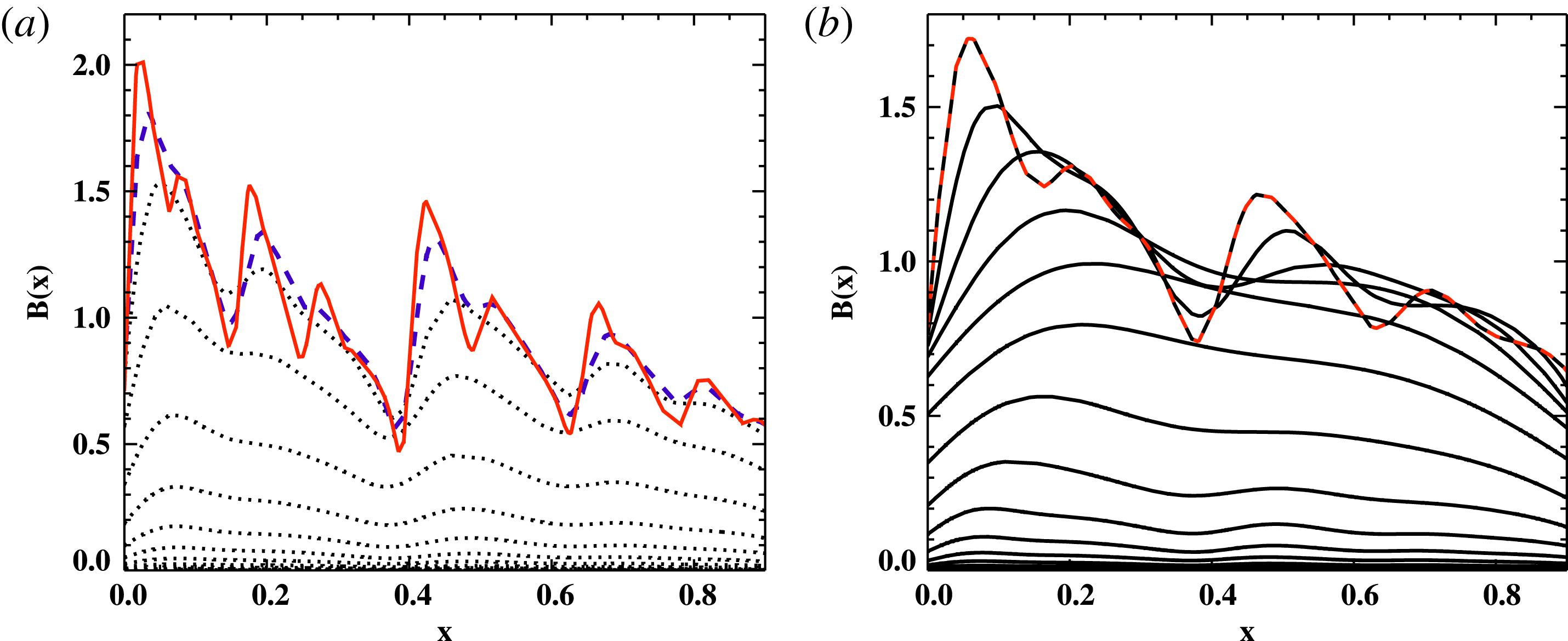
This implies that we are effectively working with a rectangle, which gets elongated further and further as the dynamo progresses. Figure 16(a) shows the evolution of a two-strip,
 $\mathit{Re}_{M}=1000$
run with such a saturation mechanism. We can see that the last few iterations overlap, indicating the onset of saturation. While the magnetic energy saturates as seen in figure 15 in curve (e), such a process eventually becomes unstable in
 $B(x)$
. This is because, as the run progresses, the map grows in the
 $x$
direction and diminishes continuously in the
 $y$
direction, thus making the diffusion step progressively inefficient. This tends to a scenario wherein the effective
 $\mathit{Re}_{M}$
for the map keeps increasing, leading to the ideal case in figure 3. The
 $B(x)$
value seems to acquire more and more structures, as can be seen in the final two curves in dashed blue and solid red in figure 16(a), reflecting the scenario of growing effective
 $\mathit{Re}_{M}$
.
Comparison of
 $B_{rms}$
for various cases. (a)–(d) Saturation by combining both decreasing
 $\mathit{Re}_{M}$
and stretching: (a) two-strip map with initial
 $\mathit{Re}_{M}=10^{6}$
,
 $c_{1}=0.1$
,
 $c_{2}=0.9$
; (b) two-strip map with initial
 $\mathit{Re}_{M}=10^{6}$
,
 $c_{1}=0.001$
,
 $c_{2}=0.999$
; (c) two-strip map with initial
 $\mathit{Re}_{M}=10^{4}$
,
 $c_{1}=0.001$
,
 $c_{2}=0.999$
; and (d) four-strip map with initial
 $\mathit{Re}_{M}=10^{5}$
,
 $c_{1}=0.001$
,
 $c_{2}=0.999$
. (e) Two-strip map with initial
 $\mathit{Re}_{M}=10^{3}$
, saturation by decreasing stretching (by changing map). (f) Two-strip map with initial
 $\mathit{Re}_{M}=10^{3}$
, saturation by decreasing stretching (by changing map) and also decreasing
 $\mathit{Re}_{M}$
, adopting
 $c_{1}=0.1$
and
 $c_{2}=0.9$
.

The evolution of
 $B(x)$
in a two-strip map dynamo,
 $\mathit{Re}_{M}=1000$
in two cases. (a) Saturation by only reduced stretching with changed map. The last two iterations have been shown as dashed blue line and solid red line. (b) Saturation by reduced stretching with changed map along with decreasing
 $\mathit{Re}_{M}$
, with
 $c_{1}=0.1$
and
 $c_{2}=0.9$
. The final iteration is shown in dashed red line.

In the flux tube picture, the flux tube will keep thickening and simultaneously grow smaller in size (radius). But, at some point, this process will have to stop when the two dimensions become comparable. Of course, the other possibility is that, when the field grows to sufficiently high values, the tension in the flux tube will not allow further twisting and folding. One way of implementing a suppression in twisting and folding is to stop the map when
 $B_{rms}$
exceeds a threshold and allow for only diffusion. Although we have not explicitly shown this here, we expect that
 $B(x)$
will freeze to its form when it first crosses the threshold in
 $B_{rms}$
, thus retaining some structures from the kinematic eigenfunction.
5.3. Saturation by combining decreasing both
$\mathit{Re}_{M}$
and stretching

We now consider the saturation of the STF map dynamo, when the effects of decreasing effective
 $\mathit{Re}_{M}$
(due to increasing renormalized resistivity) and decreasing stretching efficiency are combined. We model this by introducing efficiency parameters
 $c_{1}$
and
 $c_{2}$
into (5.1) and (5.2). We adopt
 $$\begin{eqnarray}\mathit{Re}_{M}=\frac{R_{M0}}{1+c_{1}R_{M0}B_{rms}^{2}},\quad {\it\alpha}={\it\alpha}_{0}(1+c_{2}B_{rms}^{2}).\end{eqnarray}$$
For
 $c_{1}=1$
and
 $c_{2}=0$
we have saturation purely by the nonlinear decrease of
 $\mathit{Re}_{M}$
, while
 $c_{1}=0$
and
 $c_{2}=1$
corresponds to the case when saturation occurs purely due to reduced stretching. We consider now the intermediate case where both
 $c_{1}$
and
 $c_{2}$
are non-zero.
The evolution of
 $B(x,t)$
of the two-strip map, adopting initial
 ${\it\alpha}_{0}=0.4$
and
 $R_{M0}=10^{6}$
, is shown in figure 17, for two cases. Figure 17(a) shows the result of adopting
 $c_{1}=0.1$
and
 $c_{2}=0.9$
(case A), while figure 17(b) shows the case when
 $c_{1}=0.001$
and
 $c_{2}=0.999$
(case B). The effective magnetic Reynolds numbers at saturation have now reduced from
 $R_{M0}=10^{6}$
to
 $\mathit{Re}_{M}=R_{\mathit{sat}}=18$
and
 $\mathit{Re}_{M}=R_{\mathit{sat}}=1066$
, for cases A and B, respectively. The corresponding kinematic eigenfunctions are shown as dashed lines in the figure. Remarkably, we see from figure 17 that the shape of
 $B(x)$
at saturation for both cases now closely matches that of the corresponding kinematic eigenfunction for
 $\mathit{Re}_{M}=R_{\mathit{sat}}$
. Thus when both the effective diffusion of the field and the stretching efficiency are affected by Lorentz forces, as would perhaps be most realistic, then the dynamo saturates with an intermediate spatial structure, that of the kinematic eigenfunction with
 $\mathit{Re}_{M}=R_{\mathit{sat}}$
with
 $R_{M0}>R_{\mathit{sat}}>R_{\mathit{crit}}$
. The
 $R_{\mathit{sat}}$
value is determined by the relative importance of the increased diffusion versus the reduced stretching. However, a change in
 $c_{1}$
has a more dramatic effect than an equal change in
 $c_{2}$
, as
 $c_{1}$
appears in an exponential function, the Gaussian in (3.7) involved in convolution to incorporate resistive effects. In figure 15, we show saturation levels of the two runs in curves (a) and (b), which are close to a value of order unity. We also show the curve (c) for a run with lower
 $\mathit{Re}_{M}=10^{4}$
, which saturates to a similar level.
The nonlinear evolution of
 $B(x)$
of the two-strip map, due to saturation by combining both increased diffusion and reduced stretching (without changing the map), adopting initial
 ${\it\alpha}_{0}=0.4$
and
 $\mathit{Re}_{M}=10^{6}$
. (a) The result of adopting
 $c_{1}=0.1$
and
 $c_{2}=0.9$
(case A); (b) the case when
 $c_{1}=0.001$
and
 $c_{2}=0.999$
(case B). The effective magnetic Reynolds number at saturation is
 $R_{\mathit{sat}}=18$
and
 $R_{\mathit{sat}}=1066$
, for cases A and B, respectively. The corresponding kinematic eigenfunctions are shown as dashed lines in the panels. We see that the shape of
 $B(x)$
at saturation closely matches that of the kinematic eigenfunction for
 $\mathit{Re}_{M}=R_{\mathit{sat}}$
. (c,d) The magnetic power spectrum,
 $M(k)$
, for the two cases, respectively. The bold black line shows
 $M(k)$
in the kinematic regime and the red dashed line is the saturated case.

We also show the magnetic power spectrum,
 $M(k)$
, in figure 17(c,d). For the case A, the saturated spectrum is smooth and increases monotonically towards smaller
 $k$
. In case B, the saturated spectrum seems to still retain some peaks near
 $k\sim 5$
and is flatter near
 $k\sim 1{-}3$
, unlike case A. This reflects the nature of the field as expected for their corresponding lower and higher
 $R_{\mathit{sat}}$
of 18 and 1066, respectively.
In the four-strip map dynamo, this kind of saturation mechanism, with coefficients
 $c_{1}=0.001$
and
 $c_{2}=0.999$
, leads to large oscillations in the form of
 $B(x)$
similar to the case when the saturation was only by reduced stretching. The field gets quite ordered by saturation as a result of inclusion of the mechanism of increased resistivity even though the value of
 $c_{1}$
is very small. These oscillations are also reflected in the evolution curve of
 $B_{rms}$
in figure 15 in curve (d).
Finally, we have also considered a case where we combine the two saturation mechanisms and at the same time change the map. The resulting
 $B(x)$
evolution is shown in figure 16(b) adopting
 $c_{1}=0.1$
and
 $c_{2}=0.9$
, with
 $\mathit{Re}_{M}=1000$
, for a two-strip map dynamo. Compared to the case in figure 16(a),
 $B(x)$
saturates to a smoother kinematic eigenfunction, but then the diffusion becomes less and less important, causing the field to develop finer-scale structures, while its r.m.s. value still maintains a steady state as seen in curve (f) of figure 15.
6. Conclusions
We have explored here the evolution and saturation behaviour of map dynamos used by Finn & Ott (Reference Finn and Ott1988, Reference Finn and Ott1990) to model Zeldovich’s STF dynamo. One of our aims is to use these simpler systems to develop some intuitive understanding of the saturation behaviour of more realistic fluctuation dynamos. The use of maps also allows one to analyse dynamos with very high values of
 $\mathit{Re}_{M}$
, much higher than what can be achieved in DNS.
We have considered in particular two types of generalized Baker’s maps, the two-strip map, where there is constant constructive folding, and the four-strip map, which allows the possibility of reversal of the field. In the absence of diffusion, the magnetic field
 $B(x)$
generated by the map dynamo develops fractal structures (Finn & Ott Reference Finn and Ott1988, Reference Finn and Ott1990). On including a diffusive step in the map, parametrized by the magnetic Reynolds number
 $\mathit{Re}_{M}$
, we find that the magnetic field
 $B(x)$
latches on to an eigenfunction of the map dynamo and is amplified only above a critical
 $\mathit{Re}_{M}=R_{\mathit{crit}}\sim 4$
for both types of dynamos. The spatial structure of the growing
 $B(x)$
also becomes shape-invariant (with iteration number), but whose complexity increases with increasing
 $\mathit{Re}_{M}$
. Such an eigenfunction is obtained independently of the initial field configuration, as we illustrated with an initial random seed field. The kinematic eigenfunction of the four-strip map shows reversals of the field, whose number increases with
 $\mathit{Re}_{M}$
. These results are similar to those presented in Finn & Ott (Reference Finn and Ott1988, Reference Finn and Ott1990) on the kinematic stage of the map dynamos, wherever the comparisons can be made. We have also illustrated both the kinematic and saturated structure of
 $B(x)$
by considering its power spectrum
 $M(k)$
. In the kinematic case, the fractal nature of
 $B(x)$
till the diffusive scale is reflected in sharp peaks in
 $k$
-space.
We then explored different ways by which the STF map dynamos could saturate. Saturation can occur due to a renormalized increase of the effective resistivity or by decreasing
 $\mathit{Re}_{M}$
. Such an effect obtains in a model where the Lorentz forces leads to an ‘ambipolar’-type nonlinear drift velocity (Subramanian Reference Subramanian1999). For both the two-strip map and the four-strip map that includes field reversals,
 $B(x)$
in the saturated state goes back to the marginal eigenfunction that would obtain for the critical
 $\mathit{Re}_{M}=R_{\mathit{crit}}$
. The structure developed during the kinematic stage is lost on saturation, and thus one can conclude that the energy is being effectively transferred to the larger scales due to nonlinear evolution, as can also be seen from their power spectra. This is analogous to the analytical results of Subramanian (Reference Subramanian1999) and the DNS results of Haugen et al. (Reference Haugen, Brandenburg and Dobler2004), Bhat & Subramanian (Reference Bhat and Subramanian2013) and Eyink et al. (Reference Eyink, Vishniac, Lalescu, Aluie, Kanov, Bürger, Burns, Meneveau and Szalay2013) for fluctuation dynamos with
 $\mathit{Pr}_{M}=1$
.
We have also explored the saturation of the dynamo when the effect of Lorentz forces is to decrease the efficiency of field amplification by stretching. This is implemented in two ways: (i) by not changing the map and (ii) when the map is changed to reflect the decreasing physical length (radius) of the flux tube and its increasing thickness.
For the two-strip map, in case (i), we show that
 $B(x)$
now saturates, preserving the structure of the kinematic eigenfunction obtained using the initial
 $\mathit{Re}_{M}=R_{M0}$
.
In case (ii), where we implement reduced stretching in the map, the magnetic energy (or
 $B_{rms}$
) saturates, but the fractal structures in
 $B(x)$
keep growing as in the ideal limit. Thus energy is still preserved at the smallest scales that survive resistive diffusion. This is analogous to the results of Schekochihin et al. (Reference Schekochihin, Cowley, Taylor, Maron and McWilliams2004) for the large-
 $\mathit{Pr}_{M}$
and small-
 $\mathit{Re}$
fluctuation dynamo, where power on resistive scales appears to be preserved during saturation. However, an intermediate behaviour obtains when the two saturation mechanisms operate in tandem. The saturated
 $B(x)$
has now the spatial structure of a kinematic eigenfunction with an intermediate
 $\mathit{Re}_{M}=R_{\mathit{sat}}$
where
 $R_{M0}>R_{\mathit{sat}}>R_{\mathit{crit}}$
. Even a small increase in the effective diffusion with growing field (with
 $c_{1}\ll 1$
) significantly smoothens the spatial structure of the field. For the four-strip map, saturation due to decreased stretching efficiency with or without increased diffusion leads to a more complicated behaviour, as now the saturated
 $B(x)$
oscillates with time, although with a structure similar to the kinematic eigenfunction.
One could have naively expected that
 $B(x)$
is driven to a universal form on saturation. However, it appears that the field structure when dynamos saturate is a non-trivial issue even for the simple map dynamos, and depends on the exact manner of saturation. The two natural possibilities, that the saturated eigenfunction approaches the marginal eigenfunction or remains of the same form as the kinematic eigenfunction, are both realized for different modes of saturation. If one takes a hint from such map dynamos, then, even for the fluctuation dynamo in a random flow, the structure of the saturated state could depend on the control parameters of the system, such as
 $\mathit{Re}_{M}$
,
 $\mathit{Re}$
and
 $R_{\mathit{crit}}$
. It would be interesting to explore such issues further. It would also be interesting to extend the map dynamos to incorporate a range of length scales, so as to mimic more realistically a turbulent flow with a range of eddy scales, and study their saturation behaviour.
Acknowledgements
A.S. thanks IUCAA for hospitality during his visits there under the Visiting Student Programme. P.B. acknowledges support from CSIR. We acknowledge the use of the high-performance computing facility at IUCAA. We thank the two referees for useful comments, which have led to many improvements in the paper, and Professor A. D. Gangal for sharing his thoughts on the Fourier analysis of fractals.