Irrigation water demand and implications for water pricing policy in rural China

QIUQIONG HUANG; SCOTT ROZELLE; RICHARD HOWITT; JINXIA WANG; JIKUN HUANG

doi:10.1017/S1355770X10000070

Irrigation water demand and implications for water pricing policy in rural China

Published online by Cambridge University Press: 26 February 2010

JINXIA WANG and

QIUQIONG HUANG: Affiliation:
Department of Applied Economics, University of Minnesota, Classroom Office Building 249e, 1994 Buford Ave. St. Paul, MN 55108, USA. Tel: (612) 624-1692. Fax: (612) 625-6245. Email: qhuang@umn.edu
SCOTT ROZELLE: Affiliation:
Shorenstein Asia Pacific Research Center, Freeman Spogli Institute, Stanford University, Stanford, CA, USA. Email: rozelle@stanford.edu
RICHARD HOWITT: Affiliation:
Department of Agricultural and Resource Economics, University of California, Davis, CA, USA. Email: howitt@primal.ucdavis.edu
JINXIA WANG: Affiliation:
Center for Chinese Agricultural Policy, Institute of Geographical Sciences and Natural Resources Research, Chinese Academy of Sciences, Beijing, China. Email: jxwang.ccap@igsnrr.ac.cn
JIKUN HUANG: Affiliation:
Center for Chinese Agricultural Policy, Institute of Geographical Sciences and Natural Resources Research, Chinese Academy of Sciences, China. Email: jkhuang.ccap@igsnrr.ac.cn

Article contents

Abstract
Introduction
Data description
Nature of irrigation water demand in northern China
Household water demand framework
Estimation strategy
Effectiveness and impacts of water pricing policies in rural China
Conclusions
Footnotes
References

Rights & Permissions

Abstract

The goal of this paper is to analyze whether reforming groundwater pricing has the potential to encourage water conservation and assess its impacts on crop production and producer income in rural China. Household-level water demands are estimated so that adjustments at both the intensive and extensive margins are captured. The results show that a large gap exists between the cost of water and the value of water to producers. Simulation analysis shows that reforming water pricing can induce water savings. However, the price of water needs to be raised to a relatively high level. We also find that the value-based policy is more effective than the cost-based policy since it generates larger water savings, given the same increase in the average price of water. While raising the price of water negatively affects crop production and crop income, higher water prices do not adversely affect the distribution of household income.

Information

Type: Research Article
Information: Environment and Development Economics , Volume 15 , Issue 3 , June 2010 , pp. 293 - 319

DOI: https://doi.org/10.1017/S1355770X10000070 [Opens in a new window]
Copyright: Copyright © Cambridge University Press 2010

1. Introduction

Water scarcity is one of the key problems affecting northern China. Past projects have tapped almost all of northern China's surface water resources. With the diminishing supplies of surface water, groundwater has played an increasingly important role in the region's economic growth. In 2007, on average, 37 per cent of total water supply came from groundwater (Ministry of Water Resources [MWR], 2008). Agriculture relies even more heavily on groundwater. With the exception of rice, at least 70 per cent of the sown area of grains and other staple crops are irrigated by groundwater (Wang et al., Reference Wang, Blanke, Huang, Huang, Giordano and Villholth2007). However, the rapidly growing industrial and urban sectors are beginning to compete with the agricultural sector for water. As a result, groundwater resources are diminishing in large areas of northern China (MWR, World Bank, and AusAID, 2001).

After several decades of past water policies that focused on increasing water supply by constructing more canals and larger reservoirs (Ross, Reference Ross1983), China's leaders have started to recognize the need to stem the rising demand for water (Boxer, Reference Boxer2001). In 2006, the government set the target for water saving for the 12th five-year plan period (2006–2010); water use per GDP should be reduced by 20 per cent relative to the 2005 level (National Development and Reform Commission et al., 2006). Since agriculture is the main water-using sector in China (62 per cent in 2007; MWR, 2008), a large portion of the water saving has been slated to come from the agricultural sector. Unfortunately, past policy efforts in promoting a number of different types of water-saving initiatives (such as the extension of water-saving technologies) have not succeeded. For example, the proportion of sown area for which farm households adopted sprinkler irrigation was only 3 per cent in northern China in 2004 (Blanke et al., Reference Blanke, Rozelle, Lohmar, Wang and Huang2007).

When trying to explain why past policy efforts have not been effective, researchers invariably have pointed to the absence of economic incentives facing water users (Lohmar et al., Reference Lohmar, Wang, Rozelle, Huang and Dawe2003; Yang et al., Reference Yang, Zhang and Zehnder2003). Similar to the situation in many places around the world, the price of irrigation water is low in China. Surface water is priced between 30 per cent and 50 per cent of the cost of supply (Zheng, Reference Zheng2002) and fees are assessed based on the size of the irrigated area. When the price of water is low and not related to the quantities demanded, the benefit from saving water is low or nonexistent. Groundwater users only need to pay for the cost of energy to pump water. No extraction fees are charged for water itself. Neither the price of surface water nor the price of groundwater played the economic role of signaling the scarcity rent.Footnote ¹ Under such a pricing scheme, users do not have any incentive to save water since the benefit of using water far exceeds the cost they pay.

Under these circumstances, China's water officials have begun to consider reforming the pricing of irrigation water as a key policy instrument for dealing with the nation's water scarcity problem (Wei, Reference Wei2001). The objective of the reform is to provide agricultural users with economic incentives to save water through higher water prices. In particular, local governments are encouraged to reform the way they price groundwater so as to better reflect the scarcity of groundwater resources (National Development and Reform Commission et al., 2006).

While there is increasing consensus that reforming water pricing is necessary, two basic issues need to be addressed before any new policies can be made. The first issue is the effectiveness of increasing the cost of irrigation. Previous economic studies in several developed countries have shown that demand for irrigation water is inelastic (e.g., Ogg and Gollehon, Reference Ogg and Gollehon1989; Moore et al., Reference Moore, Gollehon and Carey1994; Schoengold et al., Reference Schoengold, Sunding and Moreno2006). If water users in China are not responsive either, raising the price of water will not significantly reduce demand. The second issue is the potential lower production that may affect China's food security and subsequent income losses producers would suffer from higher irrigation costs. The current government is intent on raising rural incomes (Lohmar et al., Reference Lohmar, Wang, Rozelle, Huang and Dawe2003); hence, it is imperative to assess how much producers would be hurt should pricing policies be effectively implemented.

The goal of this paper is to analyze whether reforming groundwater pricing has the potential to encourage water conservation and assess its impacts on crop production and producer income in rural China. To meet this goal, we develop an approach that can inform policymakers about the responsiveness of household water users and assessing the magnitudes of the water price increments that are required to achieve the water saving targets of policymakers. Unlike most previous studies, we first assess whether or not the current price of water reflects the value of water. To do so, we estimate a set of county-level, crop-specific production frontiers, as well as household-level technical efficiency parameters. The results indicate a large gap between the cost of water and the value of water to producers. We then proceed to examine the effects of water pricing policy on water savings using a series of simulation analyses.Footnote ² In particular, we examine two different water pricing policies, one that takes into account the gap between the cost of water and the water value (henceforth, the value-based policy); the other that ignores this gap (henceforth, the cost-based policy). Finally, we analyze the impacts of water pricing policy on crop production (especially the production of grain crops) and producer income.

The contributions of this paper are two-fold. First, this paper is one of the few quantitative studies of water demand that can be used to advise policymakers. Only a few studies have attempted to analyze water demand in rural China (e.g., Yang et al., Reference Yang, Zhang and Zehnder2003; Chen et al., Reference Chen, Zhang, Sun, Liu, Wang and Savenije2005) and most are only qualitative. Second, to our knowledge, this paper is the only study that analyzes water demand in rural China using household level survey data. Our approach of estimating water demand at the household level characterizes the responsiveness of water users more accurately for two reasons. The decision on irrigation water use is made at the household level. Moreover, households often grow multiple crops and adjust their water use either by reducing water use per unit of land or by reallocating irrigated land among crops.

The rest of the paper is organized as follows: In section 2, we describe the data, and in section 3, we describe the relationship between water cost and water use that we observe in the data. In section 4, we introduce the framework for studying household water demand, while in section 5, we describe the estimation approach. The results of the estimation are reported and used in section 6 to simulate the effects of raising water prices. Section 7 concludes the paper.

2. Data description

The data used in the study come from the 2004 China Water Institutions and Management (CWIM) survey, which was jointly run by the authors. We collected household level data in 24 communities in Hebei province, a province that covers most of the Hai River Basin (HRB) and surrounds Beijing. The communities were chosen randomly from three counties that were also randomly selected according to their locations, which were correlated with the extent of water scarcity in the HRB. Xian County is located along the coastal belt (the most water-scarce area of China), Tang County is located along the inland belt (an area with relatively abundant water resources since it is next to the mountains in the western part of Hebei province), and Ci County is located in between the coast and mountains.

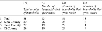
In the survey, we collected data on household-level production activities, in particular, irrigation water use, during year 2004. The major crops in Hebei province are wheat, maize, and cotton. The numbers of sample households that grew each crop are reported in table 1. For each crop, we collected information on yields, crop prices, costs, and quantities of each type of input: fertilizer, labor (by production activity), machinery (use of own equipment or rent), pesticide, plastic sheeting, etc.

Table 1.

Number of sample households that grew wheat, maize, or cotton, Hebei Province, China, 2004

Data source: Authors’ survey in 2004 (CWIM data).

Rural households in Hebei province rely on groundwater as the major source of irrigation.Footnote ³ To construct a measure of the volume of water applied, we asked households to report for each crop the length of irrigating time, the total number of irrigations during the entire growing season, and the volume of water applied per irrigation. If households were not clear about the volume of water applied, we obtained information from the manager of the well from which the household obtained the water. The managers usually were able to give us detailed information about the size of the irrigation pump and the average volume of water that each pump lifted out of the wells per hour. We then calculated the volume of water by multiplying the average volume of water pumped per hour by the length of irrigating time.

In addition, households reported the amount of money that they paid for irrigation water for each crop. In almost all communities, households paid for water according to the number of hours that the managers operated the pumps to irrigate their crop. Therefore, the cost of water is closely related to the energy cost of lifting water out of wells (either electricity or diesel). The cost of water is calculated as total payment for water divided by the volume of water used. In the rest of the paper, the cost of water and the price of water are used interchangeably.

3. Nature of irrigation water demand in northern China

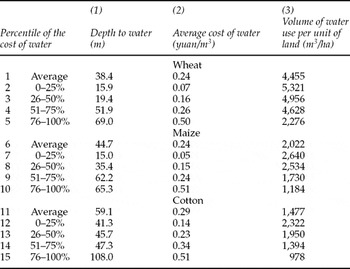
Our sample data show large variations in the price of water paid by households. Most variation in the price of water arises because the depth to water varies significantly across space, from less than 20 m to more than 100 m, as shown in table 2, column 1. Furthermore, there is a strong positive correlation between the price of water and the depth to water for wheat, maize, and cotton (columns 1 and 2). Households that paid more for water are usually those that faced greater depth to water because it cost more to pump the water out. For example, maize-growing households in the fourth quartile (those pumping from the deepest wells) paid as much as 0.51 yuan/m³ for water (column 2, row 10). In contrast, households in the first quartile paid as little as 0.05 yuan/m³ (column 2, row 7).

Table 2.

The cost of water, depth to water, and water use in Hebei Province, China, 2004

Data source: Authors’ survey in 2004 (CWIM data).

With the large variation in the price of water across space, we observe several patterns of water use. First, there is a strong inverse relationship between the price of water and the level of water use. As the price of water rises, households adjust water use by lowering their water use per unit of irrigated area. In this paper, we define this as adjustments at the intensive margin or stress irrigation. For example, wheat-growing households that face a price of 0.07 yuan/m³ water applied 5,321 m³/ha; other wheat-growing households that pay 0.5 yuan/m³ used only 2,276 m³/ha (table 2, columns 2 and 3, rows 2 and 5). The water use among households that grew maize or cotton also monotonically decrease in response to rising water prices.

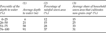
In addition to the adjustments at intensive margin, households also respond to price increases in several other ways. In particular, households may choose not to irrigate some of their crops or change their crop mix. We defined these responses as adjustments at the extensive margin. On average, households in the first quartile of depth to water left 12 per cent of their sown area to be rainfed, as shown in table 3 (row 1, column 2). The share of sown area that is rainfed increases to 37 per cent among households in the fourth quartile of depth to water (row 4, column 2).

Table 3.

The depth to water and crop mix in Hebei Province, China, 2004

Data source: Authors’ survey in 2004 (CWIM data).

^aNongrain crops include cotton, vegetables, fruits, trees, and peanuts.

Households also tend to allocate greater shares of sown area to nongrain crops as the depth to water increases. On average, households in the first quartile allocate 15 per cent of their sown area to nongrain crops (table 3, row 1, column 3). The share is more than 30 per cent for households in the third and fourth quartiles (rows 3 and 4, column 3).

4. Household water demand framework

Most of our sample households are engaged in producing multiple crops including wheat and maize (table 1, row 1). Some households also grow cotton. Our data show that households respond to changes in water prices through intensive margins as well as through extensive margins; the latter calls for analyzing water use at the household level instead of at the crop level. In this section, we lay out the framework that we use to analyze water demand at the household level.

Five inputs are used in production of crop j. Two inputs are variable inputs: material (x_kj) and fertilizer (x_fj). Material costs include expenditures on machinery, seed, plastic sheeting, herbicides, and pesticides.Footnote ⁴ It is assumed that the farmers can purchase fertilizer at unlimited quantities at the market price. Land (x_Lj), family labor (x_lj), and water (x_wj) are treated as fixed allocatable inputs.Footnote ⁵

Households are assumed to maximize the total profit from all three crops.Footnote ⁶ Given the small sizes of farms in rural China, all households are price-takers. The constrained profit maximization problem (problem P1) can be expressed asFootnote ⁷

$\begin{equation} \begin{array}{l} \mathop {{\rm Max}}\limits_{x_{ij} } \,\sum\limits_j {p_j \theta f_j (x_{Lj} ,x_{wj} ,x_{lj} ,x_{fj} ,x_{kj} )} - \sum\limits_i {c_i x_{ij} } \\ \begin{array}{*{20}l} {{\rm Subject}\;{\rm to:}} & {\sum\limits_j {x_{ij} \le B_i } {\rm }\quad \quad \forall i = {\rm Land,}\{\rm labor,}\{\rm water}} \\ \, & {x_{ij} \ge 0,} \\ \end{array} \\ \end{array}\end{equation}$

where the output price for crop j is p_j and the production frontier for crop j is f_j. The cost for input i is c_i. B_i is the available quantity of the ith fixed allocatable input.

The parameter θ is the technical efficiency parameter that captures the degree of deviation of each household's actual production from the production frontier. More importantly, since technical efficiency is often the result of a lack of managerial ability (Farrell, Reference Farrell1957; Leibenstein, Reference Leibenstein1966), θ reflects the interhousehold differences in managerial ability. Accounting for technical efficiency is important since it can help us overcome a common problem in estimating a production function – the potential omitted variable bias. In particular, household managerial ability is often omitted because it is not directly observable to econometricians. Since the managerial ability affects both output level and the producer's choice of input, omitting it will bias the estimates of production function parameters (Griliches, Reference Griliches1957).Footnote ⁸ Fortunately, the estimated technical efficiency parameters are able to capture unobservable heterogeneity that is relevant in our analysis (that is, managerial ability). As a result, we believe that our estimates will be less affected by the omitted variable bias.

After solving problem P1, the first-order condition associated with x_wj is

(1)

$\begin{equation} p_j \theta \frac{{\partial f_j (\bullet)}}{{\partial x_{wj} }} = c_w + \lambda _w .\end{equation}$

Equation (1) shows that household water demand is determined by balancing the marginal benefit and cost of water. The marginal benefit of water is measured by the value marginal product (VMP) of irrigation water, p_j (∂f_j (•)/∂x_wj, which is also the household's valuation of irrigation water (Young, Reference Young2005). The actual cost of irrigation water that the households paid is c_w.

The actual cost, however, does not always reflect the true value of water to the households. In particular, when the water resource constraint is binding, λ_w is positive. The positive λ_w creates a gap between the VMP of water and the cost of water that the households need to pay. We can call λ_w the shadow value of water since it measures the amount a household is willing to pay to relax the water constraints by one unit.

From equation (1), it is clear that as long as c_w is not raised to the level of VMP, that is, if λ_w is nonzero, households will not change the way they use water. This is because the right-hand side of equation (1) does not change (because a higher c_w reduces the value of λ_w, while the total value of c_w + λ_w does not change). If this was the case, the effects of water pricing policy would be simply increasing the cost of irrigation without inducing any water savings. Thus, in designing a water pricing policy, the first necessary task is to determine whether there is a gap between VMP and c_w, and if so, how large the gap is.

When studying household water demand, unlike most studies, we use a two-step approach. Since λ_w measures the gap between the value of water and the actual cost of water, our first step in studying water demand is to estimate λ_w. The shadow value of water, λ_w, is measured by the increment in household profit due to one more unit of water available to households. This change in net income method has been shown to generate better estimates of water values than other approaches, especially in the presence of fixed allocatable inputs (Young, Reference Young2005). The value of water to households is calculated as the change in household profits after relaxing the water constraint by one unit while holding everything else constant (e.g., prices of inputs and output, the amount of available land, and family labor).

In the second step, we first parameterize problem P1 using estimation results. We then solve problem P1 when water prices are raised to higher levels. The simulation approach allows us to predict the extent of water savings in response to price changes that include adjustments at both the intensive margin and the extensive margin.Footnote ⁹

5. Estimation strategy

From the previous section, it is clear that to characterize household-level water demand, we need to estimate two sets of parameters: the production frontier f_j and the household-specific technical efficiency parameter θ. In this paper, the production frontier parameters are estimated using the method of generalized maximum entropy (GME) and the set of technical efficiency parameters are estimated using data envelopment analysis (DEA). Our strategy is to estimate these two sets of parameters simultaneously to increase estimation efficiency.

5.1. Production frontier and generalized maximum entropy

We estimate one set of crop-specific production function for each county, allowing production technology to vary by county, but restricting it to be equal across communities within the same county. Since the price responsiveness of water demand depends on its own- and cross-price elasticities, a flexible functional form should be used so that these relationships are not arbitrarily restricted by the choice of the functional form. We specify a quadratic function frontier, $f_j () = \sum\nolimits_i {\alpha _{ij} x_{ijn} } - \sum\nolimits_i {\sum\nolimits_{i\prime } {x_{ijn} z_{ii\prime j} x_{i\prime jn} } }$ , where n is the index for households. Then the production function of household n can be expressed as

(2)

$\begin{equation} Y_{jn} = \theta _n \left( {\sum\limits_i {\alpha _{ij} x_{ijn} } - \sum\limits_i {\sum\limits_{i'} {x_{ijn} z_{ii'j} x_{i'jn} } } } \right) + e_{jn} .\end{equation}$

The observed output and input use of household n for crop j are denoted by Y_jn and x_ijn respectively. The symbol θ_n denotes the technical efficiency of household n. The error term e_jn captures variation in outputs due to random events such as weather.

In addition to the data-consistent constraints, which are specified in equation (2), two sets of theoretical constraints are also used so that the estimated production technology is consistent with the profit maximization behavior of households. The first set is the optimality condition constraints, which is obtained by deriving the first-order condition of problem P1 using the functional form specified in equation (2) as

(3)

$\begin{eqnarray} x_{ijn} \,{=}\, \frac{1}{{2z_{iij} }}\Bigg[ {\alpha _{ij} - 2\sum\limits_{i' \ne i} {x_{i'jn} z_{ii'j} } - \frac{{c_{in} }}{{p_j \theta _n }}} \Bigg] \!{+}\, v_{ijn}\quad \forall i = {\rm Fertilizer,}\;{\rm material}{\rm .}\nonumber\\[-6pt] \end{eqnarray}$

We only include the optimality conditions for variable inputs. The optimality conditions for fixed allocatable inputs contain the shadow values, which are not directly estimatable.

The second set of theoretical constraints is the curvature constraint, which requires that Z, the matrix with elements being z _ii′js, be positive (semi)definite. The Cholesky decomposition is used (Paris and Howitt, Reference Paris and Howitt1998). The positive (semi)definiteness of Z is guaranteed by first decomposing Z into Z = LL' and then constraining the diagonal elements of L to be nonnegative, where L is a lower triangular matrix. The Cholesky decomposition also ensures the symmetry of Z. In addition, we also impose the monotonicity constraints $p_j \theta _n [ {\alpha _{ij} - 2\sum\nolimits_{i\prime } {x_{i\prime jn} z_{ii\prime j} } }] - c_{in} > 0$ .Footnote ¹⁰

5.2. Generalized maximum entropy

Estimating a flexible production frontier, however, would make the use of some estimation methods difficult or even infeasible. Since five inputs are used in production and a quadratic functional form is specified, there are 20 parameters to be estimated for each production frontier. If classical econometric methods (e.g., maximum likelihood estimation) were used, the estimation problem would be ill-posed due to insufficient number of data points. For example, when we estimate a production frontier for wheat in Tang and Ci counties, there are only 18 and 19 data points respectively (table 1, rows 3 and 4, column 2). This means that there are fewer observations than the number of parameters.

As a solution, we choose to use the GME method that was developed by Golan et al. (Reference Golan, Judge and Miller1996). The GME estimator allows for estimation with any sample size. The GME estimator emphasizes both prediction and precision in its objective function and, thus, has the properties of being both subject to limited bias and minimum variance (Golan et al., Reference Golan, Judge and Miller1996). Under very general conditions, the GME estimator also has desirable large sample properties, including both asymptotic efficiency and asymptotical normality.

Instead of directly estimating the mean and variance of the coefficient, when the GME method is used, a probability distribution is estimated for each coefficient and the error term. Several possible values of a coefficient are chosen as the support values of the probability distribution and an unknown probability is assigned to each value.Footnote ¹¹ The coefficients and the error terms are then reparameterized in terms of unknown probabilities and support values. This set of reparameterization constraints are defined as $\alpha _{ij} = \sum\nolimits_m {p_{\alpha _{ij} }^m } \bar \alpha _{ij}^m, z_{ii\prime j} = \sum\nolimits_m {p_{z_{ii\prime j} }^m } \bar z_{ii\prime j}^m, v_{ijn} = \sum\nolimits_m {p_{v_{ijn} }^m \bar v_{ijn}^m }$ , and $e_{jn} = \sum\nolimits_m {p_{e_{jn} }^m \bar e_{jn}^m }$ , where m is the index of the support values and the ps are the unknown probabilities to be estimated. Symbols with upper bars denote the support values. The unknown probabilities are positive and all probabilities associated with the same coefficient or error term add up to one (the adding up constraints).

In GME estimation, the estimates of probabilities, given their support values, are obtained through maximizing the negative of the joint entropy of the distributions of the coefficients and the error terms. The GME estimation problem (problem P2) can be summarized as

$\begin{eqnarray*} &&{\mathop {{\rm Max}}\limits_{p_{\alpha _i }^m ,p_{z_{ii'} }^m ,p_{e_n }^m ,p_{v_{in} }^m } \,H(p_{\alpha _i }^m ,p_{z_{ii'} }^m ,p_{e_n }^m ,p_{v_{in} }^m )}\\ &&\qquad = - \sum\limits_{j = 1}^J {\sum\limits_i {\sum\limits_m {p_{\alpha _{ij} }^m } \,\ln \,p_{\alpha _{ij} }^m } } - \sum\limits_{j = 1}^J {\sum\limits_i {\sum\limits_{i'} {\sum\limits_s {p_{z_{ii'j} }^m } \,\ln \,p_{z_{ii'j} }^m } } }\\ &&\qquad\quad - \sum\limits_{n = 1}^N {\sum\limits_m {p_{e_n }^m \,\ln \,p_{e_n }^m } } - \sum\limits_{n = 1}^N {\sum\limits_i {\sum\limits_m {p_{v_{in} }^m } \,\ln \,p_{v_{in} }^m } } , \end{eqnarray*}$

subject to the data-consistent constraints, the optimality condition constraints, the curvature constraints, the monotonicity constraints, the reparameterization constraints, and the adding up constraints.Footnote ¹² Note that the production frontiers of all crops are estimated jointly.

5.3. Technical efficiency parameters and data envelopment analysis

We use the Farrell definition of the output distance function to measure θ_n (Farrell, Reference Farrell1957). Using the DEA method, the technical efficiency of household n, θ_n, can be estimated through solving the following linear programming (LP) problem (problem P3) (Farrell, Reference Farrell1957; Charnes et al., Reference Charnes, Cooper and Rhodes1978; Färe and Primont, Reference Färe and Primont1995):

${\fontsize{8.7}{10.2}\selectfont{\begin{eqnarray*} \begin{array}{*{20}l} {\mathop {\rm Max}\limits_{\theta _n ,\psi _1 ,\psi _2 , \ldots ,\psi _H } \,1/\theta _n } \\ {{\rm Subject}\;{\rm to}:\left\{\!\! {\begin{array}{*{20}l} {\sum\limits_{h = 1}^H {\psi _h (Y_{jh} - e_{jh} )} \ge (Y_{jn} - e_{jn} )/\theta _n ;\quad {\rm }j = 1,2, \ldots ,J;\quad h = 1, \ldots ,H} \\ {\sum\limits_{h = 1}^H {\psi _h (x_{ijh} } - v_{ijh} ) \le (x_{ijn} - v_{ijn} )} \\ {\sum\limits_{h = 1}^H {\psi _h } \le 1} \\ {\psi _h \ge 0, \quad h = 1, \ldots ,N,} \\ \end{array}} \right.} \\ \end{array}\end{eqnarray*}}}$

where the variable ψ_h represents the intensity level of the production activity of household h and N is the total number of households in a county. The inequality $\sum\nolimits_{h = 1}^H {\psi _h } \le 1$ is specified so that the technology exhibits nonincreasing returning to scale, which is consistent with the quadratic frontier specified in (2) (Färe and Primont, Reference Färe and Primont1995). Note that in the constraints, we subtract e_jn from Y_jn and v_ijn from x_ijn, which avoids attributing any statistical noise to deviations from the frontier, a weakness of DEA pointed out by many researchers.

5.4. Summary of estimation strategy

Our estimation strategy is to estimate the production frontier parameters (using GME) and the technical efficiency parameters (using DEA) simultaneously. This is done by adding together the objective functions of problems P2 and P3 of all households. The joint estimation has been done in several previous studies (Oude Lansink et al., Reference Oude Lansink, Silva and Stefanou2001; Karagiannis et al., Reference Karagiannis, Tzouvelekas and Xepapadeas2003; Campbell et al., Reference Campbell, Rogers and Rezek2008), but has not been used extensively in analyzing water demand. In summary, our estimation problem (problem P4) can be expressed as

${\fontsize{9}{10.5}\selectfont{\begin{eqnarray*} &&\mathop {{\rm Max}}\limits_{p_{\alpha _i }^m ,p_{z_{ii'} }^m ,p_{e_n }^m ,p_{v_{in} }^m ,\theta _n } - \sum\limits_{j = 1}^J {\sum\limits_i {\sum\limits_m {p_{\alpha _{ij} }^m } \,\ln \,p_{\alpha _{ij} }^m } } - \sum\limits_{j = 1}^J {\sum\limits_i {\sum\limits_{i'} {\sum\limits_s {p_{z_{ii'j} }^m } \,\ln \,p_{z_{ii'j} }^m } } } \\ &&\qquad - \sum\limits_{n = 1}^N {\sum\limits_m {p_{e_n }^m \,\ln \,p_{e_n }^m } } - \sum\limits_{n = 1}^N {\sum\limits_i {\sum\limits_m {p_{v_{in} }^m } \,\ln \,p_{v_{in} }^m } } \\ &&\quad \quad + 1/\theta _1 + 1/\theta _2 + \cdots + 1/\theta _n + \cdots + 1/\theta _N .\end{eqnarray*}}}$

Problem P4 is subject to all the constraints in problems P2 and P3. Solving problem P4 is analogous to estimating a system of equations in classical econometrics. For example, when full-information maximum likelihood (FIML) is used, the objective function is the likelihood function that represents joint probability density of data from multiple equations. Similar to the reason that FIML is more efficient than single-equation estimation methods, our strategy of simultaneously estimating the two sets of parameters also generates more efficient estimates.

The use of DEA together with GME allows us to estimate technical efficiency and frontier parameters simultaneously. This is true for three reasons. First, constraints used in the DEA approach are consistent with the theoretical constraints (concavity and monotonicity) in the GME estimation approach. The constraints in the LP problem specify disposability, which corresponds to the monotonicity of the production frontier and the convexity of the feasible production set, which corresponds to the concavity of the frontier. Second, the simultaneous estimation of the technical efficiency parameters and the frontier parameters can be done with ease. This is because the objective function of the LP problem in DEA and its constraints are easily incorporated into those of the GME framework since GME is also solved through a maximization problem. Third, bootstrapping can be used to obtain standard errors of technical efficiency and frontier coefficients simultaneously. Bootstrapping is often used in GME estimation to obtain standard errors of coefficients. A series of papers by Simar and Wilson (Reference Simar and Wilson2000a, Reference Simar and Wilson2000b; Reference Simar and Wilson2007) developed several techniques that allow analysts to bootstrap and obtain bias-corrected estimates of technical efficiency parameters and standard errors. The DEA approach together with the Simar and Wilson bootstrapping technique generates consistent estimates of θ_n and standard errors (Kneip et al., Reference Kneip, Park and Simar1998). We used a bootstrapping procedure that combines algorithms developed in Simar and Wilson (Reference Simar and Wilson2000b; Reference Simar and Wilson2007). Details of bootstrapping are not presented here, but are available from authors upon request. Problem P4 is solved using the general algebraic modeling system (GAMS) software. STATA is used to generate bootstrapping samples.

6. Effectiveness and impacts of water pricing policies in rural China

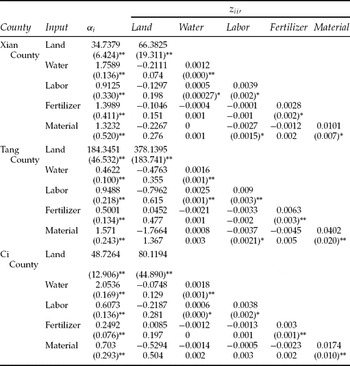
The estimation approach presented in the previous section produced reasonable estimates of the production frontier coefficients. In table 4, for the sake of brevity, we only report the results for wheat production frontiers. Bootstrapping results show that most estimates are statistically significant. The linear coefficients (the α_is) are all positive and statistically significant. The quadratic coefficients are also reasonable. For example, coefficients on the interaction term between water and labor are positive and statistically significant, indicating that water and labor are complements in all three counties. Our estimates of technical efficiency parameters range from 0.47 to 0.99 with a mean of 0.89. The statistics for estimated technical efficiency parameters (mean, minimum, and maximum) do not vary significantly across counties. The estimates have small standard errors, all within the order of magnitude of 0.001.

Table 4.

Estimation results of the wheat production frontier, $\sum\nolimits_i {\alpha _i x_i } - \sum\nolimits_i {\sum\nolimits_{i\prime } {x_i z_{ii\prime } x_{i\prime } } }$

a. For the sake of brevity, estimation results of the production frontier of maize and cotton as well as the set of technical efficiency parameters are not reported here.

b. Bootstrapped standard errors are reported in parentheses.

c. When performing the GME estimation, we change the unit of land to square meters so that the magnitude of land is in range with that of other inputs. Because of the rescaling, coefficients on land are large in magnitudes.

d. Asterisk (*), double asterisk (**), and triple asterisk (***) denote coefficients significant at 10 per cent, 5 per cent, and 1 per cent levels respectively.

In this section, we analyze the effects of water pricing policy on water use, crop production, and household income. We parameterize the household maximization problem P1 using estimation results. Treating the current costs of water as the baseline water prices, we first run a baseline model by solving problem P1 for each household. We then increase the price of water to several different levels while holding prices of other inputs and outputs constant. We solve problem P1 at each of these new water price levels. Simulation results form the basis of our policy analyses. By comparing the changes in household water use, we can predict the extent of water savings that occur when water prices are raised to different levels. Since the simulations also generate the level of crop outputs and household profits, we can also predict the impact on crop production and income.

Since wheat, maize, and cotton account for 80 per cent of total sown area in our sample, we only include these three crops in the simulations. If more crops, such as nongrain crops (e.g., vegetables and fruits), were included, households would be able to adjust more at extensive margins by switching to these crops. We also keep the same rotations, as in practice. Only wheat is grown in summer season and either cotton or maize (or both) is grown in fall season.

6.1. Effectiveness of water pricing policy: value-based policy and cost-based policy

The effectiveness of water pricing policy depends crucially on the responsiveness of households. If the water price is lower than the value of water to households, households will not change water use at all in response to small changes in water prices. Thus, a necessary task in designing a water pricing policy is to determine whether the current price of water reflects the value of water to households. This is our first step in this subsection. We then compare the effects of two types of water policies that differ in their treatment of the value of water.

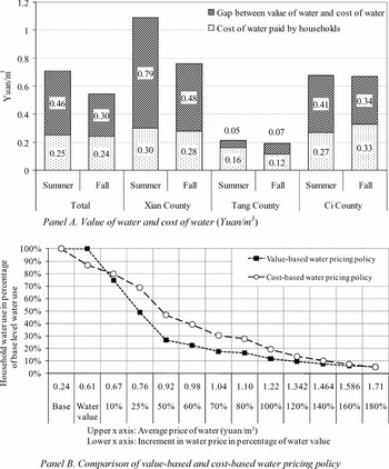
Our results show that there is a large gap between the cost of water and the value of water in most households in Xian and Ci counties (figure 1, panel A). Since resource constraints are season specific, we have calculated the value of water to households for both the summer and fall seasons. For most households in Tang County, the cost of water they paid is the same as the value of water. In Xian County, however, the gap is almost double the irrigation cost in both seasons. In Ci County, the gap is also large in both seasons.Footnote ¹³ The same finding has been observed in many other countries: water is usually underpriced and its price usually does not reflect the scarcity value (Dinar and Saleth, Reference Dinar, Saleth, Folmer and Tietenberg2005). From our results, it is clear that at least in Xian and Ci counties, households will not change their water use much in response to small increases in water prices. This is because the new price level after small increases would still be lower than the household's actual value of the water.

Figure 1.

Effects of higher water prices on household water use

Given the large gap between the price of water and the value of water, policymakers can design two types of water policies: a cost-based policy and a value-based policy. When implementing a cost-based policy, we assume that policymakers are not aware of the gap between the current water cost and the true value of water to households. As a result, officials consider the current price of water as the starting point and simply raise the price of water from there. In contrast, policymakers can first find out whether the current cost of water reflects the household's value of water. They could do so by collecting information and generating estimates of the households’ actual value of water. With such information, a value-based policy could be implemented in a two-step way. In the first step, the price of water of each household could be increased from its current level to a level that equals their value of water. In the second step, the price of water could then be increased to a point at which users would begin to cut back water use enough to meet the water saving target.

In order to make cost-based and value-based policies comparable, we make sure that the changes in the average prices of water under the two policy regimes are the same. For example, under the value-based policy scenario, when the price is first increased to the level of water value and then increased further by 50 per cent of the water value (a two-step procedure), the average price is raised by 0.68 yuan/m³ and reaches 0.92 yuan/m³. Then we also raise the price under the cost-based policy by 0.68–0.92 yuan/m³ (in one step). Since the average price of water before and after the changes under the two policies are the same, we can put changes in household water use under these two policies on the same graph and plot them against the average water prices (figure 1, panel B).

The simulation results show that the value-based policy has the potential to induce sizable water saving. By construction, households do not change water use in the first step when the cost of water is raised to equal the value of water. Once the cost of water has hit the level of water value, however, households are highly responsive to price changes. Suppose policymakers plan to reduce water by 20 per cent, which means households need to reduce their water use to 80 per cent of the base level. In order to meet the 20 per cent water savings target, after the price is increased to 0.61 yuan/m³ in the first step, the price only needs to be further raised by 10 per cent more (from 0.61 to 0.67, figure 1, panel B). In order to achieve a 50 per cent water savings target, the price of water only needs to be raised further to 0.76 yuan/m³, only 0.09 yuan/m³ higher than the level that was needed to hit a 20 per cent target. Therefore, when the price of water reflects the value of water, water pricing policy can be an effective tool in dealing with the water scarcity problem.

Our results also show that the price of water needs to be increased greatly. For example, in order to meet a 20 per cent water saving target, the average price is increased to about 0.67 yuan/m³, a 180 per cent increase from the base level. It is important to note that most of the rise in the price of water is in the first step of the value-based policy. Of the total rise of price (0.43 yuan/m³), 0.37 yuan/m³ is just needed to get all households to the point that the cost of their water is equal to the value of water. Such large price rises may conflict with other policy goals that aim at keeping food production high and lifting rural incomes. This issue is addressed in later subsections.

Comparisons indicate that when the water saving target is high, the value-based policy is the more effective water pricing policy. For example, if water officials set a target of a 50 per cent reduction in water use, under the value-based policy, the price is increased to 0.76 yuan/m³. However, to achieve a similar saving under the cost-based policy, the price would need to be raised to 0.92 yuan/m³. This is because under the cost-based policy, policymakers increase the price by an amount that is the same for all of the households, regardless of whether the household has a high or low value for water. Because of the large gaps between the cost of water and the value of water, especially in Xian County and Ci County, if the price was increased only to 0.76 yuan/m³ (the average water price under the value-based policy), it would still be below the true value of water to some of the households. These households would not respond to price changes at all, and so, the 50 per cent water saving target could not be achieved. As a result, policymakers have to raise the price to 0.92 yuan/m³ to make sure that it exceeds the level of water values of enough households to reach the target. Although the change in the average price is the same under both policies, the value-based policy increases prices in a more targeted way to make sure that all households are responsive. So, under the value-based policy, the same amount of water price increment is much more effective. In this case, following the cost-based policy would force policymakers to increase the price of water to a higher level than necessary. This higher price would not only result in higher costs for farmers, but also increase the financial burdens of the water pricing policy if policymakers planned to compensate farmers for their higher costs.

The value-based policy, however, does not always outperform the cost-based policy. When the water saving target is small (e.g., less than a 20 per cent reduction in our case, as marked by the intersection of the value-based policy and cost-based policy in the upper left corner of panel B in figure 1), the cost-based policy works more effectively in reaching the target. This is because only a small proportion of households need to be responsive in order to reach a small water saving target. Therefore, the uniform increase in water prices under the cost-based policy is sufficient. The cost-based policy works better because it does not require the large increment in water prices to get all households to the point that they are facing their actual water values as is needed in the first step of the valued-based policy.Footnote ¹⁴

Whether a value-based policy or a cost-based policy should be pursued depends on the specific water saving target, the implementation cost and other considerations. The cost of implementing a cost-based policy is probably significantly lower than that of the value-based policy since it does not involve collecting information that is needed to estimate household level water demand. So, a cost-based policy is appropriate when the water saving target is small (less than 20 per cent reduction in our case). Since the government has set the water saving target at 20 per cent in the 11th five-year plan, at least for now, the cost-based policy may be appropriate. If the water saving target is more than 20 per cent reduction, the need for a value-based policy increases. Although the cost of implementing the value-based policy at the household level may be high, implementing it at a less disaggregated level, such as the county level, may be feasible.

6.2. Impacts of water pricing policy on crop production

Although increasing the price of water has been shown to be effective in reducing water use, leaders must also take into account other impacts of higher irrigation costs. We examine how increasing the price of water will affect crop production in this subsection and producer income in the next subsection. In the rest of our analysis, we focus only on the value-based policy scenario. We run four different simulations. In each simulation, we first raise the price of water each household faces to their value of water, and then increase the price of water further by percentages of the level of water values (10 per cent, 25 per cent, 50 per cent and 100 per cent respectively).Footnote ¹⁵

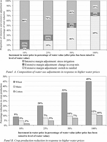
Consistent with findings from descriptive analysis, when the price of water is raised above the level of the value of water, households indeed will adjust their use of water (seen in figure 1) and these changes occur at both the intensive and extensive margins (figure 2, panel A). Importantly, when the price increment is small, most of the adjustments come from intensive margins. For example, when the price of water is increased by 10 per cent after being increased to the level of water value, about 80 per cent of the total reduction in water use comes from adjustments at intensive margins. On average, wheat producers reduce their water use per hectare from 4,436 to 3,637 m³.Footnote ¹⁶ Maize producers also cut back from 2,150 to 1,516 m³ and cotton producers from 1,653 to 1,244 m³. At the same time, adjustments at the extensive margin account for the remaining 20 per cent of the total reduction. About 3 per cent of the total change comes from shifting from irrigated to nonirrigated agriculture and 17 per cent comes from shifting the crop mix. In our case, most households shift from maize to cotton, which requires less water than maize.

Figure 2.

Effects of higher water prices on crop production under value-based water pricing policy

While most of the adjustments occur at the intensive margins when price rises are relatively small, as the price rise gets higher to target more water savings, more of the adjustments come from the extensive margins. For example, when the water price is double the level of water value (that is, a 100 per cent increment in the price), almost 75 per cent of the total water reduction comes from adjustments at extensive margins (versus 20 per cent when the price was increased by 10 per cent) (figure 2, panel A). Most changes at the extensive margin occur when farmers choose to stop irrigating their crops (69 per cent). The remaining 6 per cent comes from changing crop mix. In contrast, only 25 per cent of the fall comes from adjustments at the intensive margins.

Simulations show that adjustments at the intensive and extensive margins affect crop production in two ways. First, stress irrigation reduces the yields of all three crops. For example, when the price increment is 25 per cent of the water value, the average yields of irrigated wheat are reduced by 23.4 per cent, irrigated maize by 11 per cent and irrigated cotton by 4.8 per cent. With lower yields, the level of crop production is, of course, lower for all crops, ceteris paribus. Yield changes due to adjustments at the intensive margin, however, only partly explains why grain production changes. Adjustments at the extensive margins shift crop production from grain to nongrain crops. Grain area (the sown area of wheat and maize) is reduced by 4.3 per cent with a 25 per cent increase in water prices. Farmers also switch from irrigated area to nonirrigated area. The total irrigated area of all crops falls by 15.6 per cent. Hence, in total, when the price of water is raised by 25 per cent, grain production falls by 14.3 per cent, of which 3.5 percentage points came from changes at the extensive margin.

When accounting for both lower yields and smaller acreage that arise from rising water costs, the simulation results imply that a wide-ranging, pan-provincial water pricing policy would reduce food production in China significantly. In particular, the production of wheat is most affected. Since the growing season of maize and cotton in Hebei province coincides with the rainy season, while that of wheat does not, wheat production relies more on irrigation and falls more when the cost of irrigation rises. For example, when the price of water is doubled, wheat production is reduced by 45 per cent (figure 2, panel B), of which 32.4 percentage points come from adjustments at the extensive margin. Since Hebei province produces about 12 per cent of China's wheat output, if the value-based water policy were implemented in Hebei, the fall in wheat output would be equivalent to more than 5 per cent reduction in China's total wheat production.

6.3. Impacts of water pricing policy on producer income

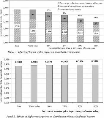
The impact of higher irrigation costs is not limited to crop production. Incomes of rural households are also lower if the water pricing policy is implemented (figure 3, panel A). In the first step of each simulation, since the real price of water each household faces (as measured by the value of water) did not change, households do not change their water use or crop production. Incomes are reduced since the actual cost of water rises and the negative effect on income of pricing policy is solely attributed to higher water prices. As can be seen when moving from bar 1 to bar 2 in panel A, on average, crop income drops by 268 yuan per household.

Figure 3.

Effects of higher water prices on produce income under value-based water pricing policy

When irrigation costs are increased during step 2, although income continued to decline due to higher water price, the rate of decline slows. For example, when policymakers increase the price of water by 10 per cent (after the initial increment in the first step), on average, crop income decreases from 1,938 yuan to 1,634 yuan (figure 3, panel A). A 10 per cent increase in the water price only drops crop income further by 30 yuan. This is because farmers are responsive to changes in water price since it reflects the value of water to them. Since farmers respond to increase in water price by reducing water use, the impact on crop income is smaller than that in the initial step. Crop income drops from 1,938 to 1,518 yuan when the price of water is doubled.Footnote ¹⁷

Hence, while water policy has great potential in saving water, the impact of water pricing policy on producer income poses a major challenge to China's policymakers in today's political economy environment. China has made remarkable progress in alleviating poverty in its rural areas in the past and the leaders are definitely intent on continuing to alleviate poverty in rural China (Rozelle et al., Reference Rozelle, Zhang, Huang, Hope, Yang and Li2003). The government has set the target of lifting 23.65 million people out of poverty in the next five years (Xinhua News Agency, 2006). With such a policy environment, there will be strong resistance against any policy that results in lower rural incomes. Almost certainly, if any water policy were to be implemented in rural China, complementary policies would be needed to offset the impacts of higher irrigation costs on rural income.

Since rural households shoulder the burden of conserving water, they should be compensated for their incomes losses. One solution is to develop a subsidy program in tandem with the water pricing policy that transfers income to households. Our results, however, show that such a policy will need outside funding, especially as the price of water is raised to higher levels. Suppose the price of water is raised through imposing a tax on per unit of water use. When the price of water is raised from its initial level to the value of water, most of the amount needed to fund the transfer program (administrative costs aside) can come from the program (the tax revenue collected). However, as the level of the water tax increases, the deadweight loss associated with the tax becomes larger. Our results show this clearly. The tax rebate can offset some income loss, but is not enough to compensate completely for the loss in crop income.Footnote ¹⁸ For example, with a 25 per cent increase in the irrigation cost, on average, each household loses 343 yuan of their crop income, while only 187 yuan per household is collected as tax (figure 3, Panel A). There is a 156-yuan gap (or 8 per cent of the base level crop income) between the income loss and the tax revenue collected. The level of the gap increases with the level of increment in the irrigation cost. When irrigation cost is doubled, the crop income loss (420 yuan) is more than six times the level of tax revenue (65 yuan). To compensate for these gaps, outside funding must be provided.

Despite its significant negative effects on average income, our simulation results show that water pricing policy does not deteriorate the distribution of income. For example, doubling irrigation cost only increases the Gini coefficient of household total income from 0.3881 to 0.391, which is only a 0.7 per cent increase (figure 3, panel B). This is consistent with findings in Dinar and Tsur (Reference Dinar and Tsur1995). In our case, one important reason for this small impact is that in rural China, land is equally allocated to households both in terms of land size and soil quality.

7. Conclusions

Tackling the growing water scarcity problem has become one of the most important tasks that China's leaders face today. Relying on a set of household level data, this paper examined the potential for conserving water through water pricing reform. Our study shows that water pricing policy has the potential of resolving the water scarcity problem in China. However, because the current cost of water is far below the true value of water in many of our sample areas, large increase in the price of water from the current level is required. For example, a reduction of 20 per cent of the current level of water use would require the water price to be more than doubled.

The difficulties of implementing water pricing are well recognized in the literature (e.g., Sampath, Reference Sampath1992; Dinar, Reference Dinar and Dinar2000). We believe, however, the cost of implementing water pricing policies in northern China may not be as high as in many other places. Almost all wells in northern China run off electric pumps. In almost all communities, households paid for water according to the number of hours that the managers operated the pumps to irrigate their crop. Therefore, groundwater is effectively volumetrically priced. Moreover, rural electricity systems are set up such that the supply of electricity can only come from one source and that source is easily monitored to prevent stealing electricity or tampering with the meters. This means that the cost of water could be raised with ease by adding a tax or fee to the price of electricity.

However, our analysis also shows that there are other costs associated with higher water prices. Higher irrigation costs will lower the production of all crops, in general, and that of grain crops, in particular. This may hurt the nation's food security goal of achieving 95 per cent self-sufficiency for all major grains in the short run. Furthermore, when facing higher irrigation costs, households suffer income losses, although income distribution does not deteriorate.

In summary, our study provides both good news and bad news to policymakers. On the one hand, water pricing policies have great potential for curbing demand and helping policymakers address the emerging water crisis. Irrigation is central for China to maintain food security in the long run and will continue to be one investment that enables China to lift its future production of food and meet its food grain security goals (Huang et al., Reference Huang, Rozelle and Rosegrant1999). The goal of water pricing policy, which is to manage water resources in a sustainable way, does not conflict with the long-run goal of the nation's food security policy. On the other hand, dealing with the negative production and income impacts of higher irrigation cost will pose a number of challenges to policymakers, at least in the short run.

One possible solution is to set a water saving target in the agricultural sector to be below the national target of 20 per cent.Footnote ¹⁹ Other sectors (e.g., industrial and residential sectors) can have the options to recycle water use for industrial use, but the recycling options are limited for agricultural producers. When the congruence of the water policy is taken with the poverty reduction and agricultural production self-sufficiency, shooting for a less than 20 per cent reduction in water use for agriculture can mitigate the damage to rural income and agricultural production.

In addition to setting a modest water saving target, if China's leaders plan to increase water prices to address the nation's water crisis, an integrated package of policies will be needed to achieve water savings without hurting rural incomes or national food security. One solution is to develop a subsidy program in tandem with the water pricing policy that transfers income to households. A subsidy program is a realistic solution in China's political economy environment. China's agricultural policy has gradually switched from taxing farmers to directly subsidizing farmers. The tax-for-free reform that targets at eventual elimination of taxation on rural households has been implemented over the past decades (Brandt et al., Reference Brandt, Rozelle and Zhang2005). The Chinese government has also started to provide nationwide direct subsidies for farmers, including direct payments to grain producers based on planting areas, direct subsidies to purchased farm inputs, subsidies to seeds, and subsidies to agricultural machineries. These subsidies amounted to RMB 31 billion (US$3.8 billion) and 42.7 billion (US$ 5.2 billion) in 2006 and 2007 respectively (Yu and Jensen, Reference Yu and Jensen2009). The “No. 1 documents” (the most important policy statements issued by China's central government) of recent years (including the year 2009) continue to promote direct farm subsidies as essential instruments in increasing rural incomes. Hence, a subsidy program is well in line with the government's policy agenda.Footnote ²⁰

Footnotes

¹ Dinar and Saleth (Reference Dinar, Saleth, Folmer and Tietenberg2005) summarized the two key roles of the price of water. The first is a financial role to recover the cost of supplying water. The second is an economic role to signal scarcity. However, in the literature, the efficient/first-best pricing method often refers to marginal-cost pricing (MCP), where water is priced at its marginal cost of supply (Dinar, Reference Dinar and Dinar2000; Tsur et al., Reference Tsur, Dinar, Doukkali and Roe2004). MCP does not consider the economic role of water price.

Scarcity rents measure the in situ scarcity of a resource. In the case of groundwater, scarcity rents reflect the opportunity cost associated with the unavailability in a future time period of a unit of water used in the present (Koundouri, Reference Koundouri2004). The social cost of pumping groundwater is generated by the externalities that arise when the pumping of one user imposes a cost on another (Provencher and Burt, Reference Provencher and Burt1993). One of the major components in the social cost is the higher cost of future pumping due to a smaller groundwater stock that results from current pumping.

² It should be noted that the objective of this study is not to determine the efficient or optimal level of the price of water. To determine the efficient price of water we would need to estimate the scarcity rent and the social cost of pumping (Koundouri, Reference Koundouri2004). However, a scarcity rent can only be observed when there is a competitive market for groundwater (Lynne, Reference Lynne1989) – which does not exist in northern China. Because of the difficulty of estimating scarcity rent, it is often ignored (Koundouri, Reference Koundouri2004). One exception is Koundouri and Xepapadeas (Reference Koundouri and Xepapadeas2004). Social cost is also difficult to estimate. Because the estimates of scarcity rents and social costs are difficult or impossible to obtain, any policy analysis based on such error-ridden estimates would not be useful. Instead, we focus on assessing the magnitude of water price increments that are required to achieve the water saving targets of policymakers.

³ All groundwater irrigation activities are organized within the community. Above level governments (e.g., the town or county) and regional water agencies (such as, irrigation districts) are rarely involved in the daily management.

⁴ In our data, the expenditure on machinery measures the flow of capital services, not the stock of capital. During the survey, if a household rent machinery for plowing, sowing, or harvesting crops, the renting cost (include the cost of energy and the cost of hiring labor to drive the tractor) was included in the expenditure on machinery. If a household owned machinery, the cost of energy was included. Furthermore, Chinese agriculture is characterized by small-scale, labor-intensive operations using little physical capital. The farm size is small in China. In our sample data, the median farm size (land holdings per household) was 0.6 ha. Mostly due to the small farm size, the level of capital asset in farming is also small in rural China. In our sample data, the median value of capital asset (the sum of the value of farm machinery and draft animals, etc.) was only 2,523 yuan per household (about $315) in 2004. Because of this, the expenditure on machinery is not a large part of the production cost. Therefore, we group the expenditure on machinery with expenditures on other material inputs and treat it as a variable input.

⁵ In rural China, the collective (or community) allocates land among households based upon household size. Since only a small proportion of plots are rented (about 3% in 1995 and 7% in 2000) (Brandt et al., Reference Brandt, Rozelle and Turner2004), we assume there is no cost for land, but that it is fixed. In addition to family labor, which is fixed by definition, labor input also may include hired labor (x_hl). Since only a small percentage of farm labor is hired in rural China (Benjamin and Brandt, Reference Benjamin and Brandt2002), it is reasonable to assume that labor is largely a fixed input. While there are no formal restrictions on pumping in the sample communities, our data show that in some communities the quantity of groundwater may be constrained, at least during the irrigation season.

⁶ In our preliminary analysis, we assume households were risk averse. The estimated risk aversion parameter is not statistically different from zero. Therefore, without loss of generality, we assume households are risk neutral.

⁷ Since there is no regulation on pumping, groundwater is a common-property resource in rural China. The large number of users (on average 500 households per community and 30 households per well in our sample) also implies that households are myopic users and only maximize profit from the current period.

⁸ Conventional panel data models, such as fixed-effects or random-effects models, have been employed to account for unobserved heterogeneity. Unfortunately, for most households in our sample, we do not have more than one observation for a single crop. Therefore, it is not possible to use a household fixed effects approach.

⁹ Moore et al. (Reference Moore, Gollehon and Carey1994) used a rigorous econometric approach to calculate the intensive and extensive margins. In our case, since large price changes, instead of marginal increments, are more relevant, simulations are more appropriate.

¹⁰ In our empirical estimation, the monotonicity constraints hold for all observations.

¹¹ We follow Golan et al. (Reference Golan, Judge and Miller1996) and choose five support points for both coefficients and error terms.

¹² We believe that our approach of estimating the production frontier does not suffer from the fundamental identification problems raised by Marschak and Andrews (Reference Marschak and Andrews1944) for several reasons. First, a system of equations is estimated including both the production frontier equation and the optimality condition equations. Second, in a separate set of analyses, we instrumented for inputs using a set of variables (input prices, whether there is a production shock or not, distance from house to plots, etc.), the results do not differ much from the case using the raw input uses. Third, since levels of output used in estimation (after correcting for the impacts of production shocks) are close to the expected levels of outputs, we believe there is no simultaneous equation bias pointed out by Hoch (Reference Hoch1958), which is associated with using actual output instead of expected output in estimation. Finally, the reasonable range out-of-prediction errors (not reported here) further shows that there is no serious bias in our estimates. This confirms what Golan (Reference Golan, Judge and Miller1996) has stated, ‘this formulation (of GME estimation) may lead to parameter estimates that are slightly biased but have excellent precision’.

¹³ The large gaps in Xian and Ci counties are consistent with findings from our survey. When asked whether there was sufficient water in the wells to meet demand during the irrigation seasons for 2002, 2003, and 2004, 13 out of 24 community leaders said there was not. Most of these communities are located in Xian and Ci counties. The constraints on groundwater arise from both the increasing water demand and the rapidly declining groundwater levels in these communities. Since water resources are scarce in Xian and Ci counties and prices do not reflect the scarcity of water, it is not surprising to find large gaps between the current costs of water and the value of water.

¹⁴ When the water saving target is ambitious (e.g., more than 90% in our case), there is also not much difference between the performance of the two pricing policies. This is because a large price increment would be needed to meet such a target under either policy (about 120% of the water value even under the value-based policy in our case, panel B). Then, it is likely the price level reaches or exceeds the value of water to most households. Consequently, most households would be responsive under either type of policy, which results in little difference between the two.

¹⁵ Because water use does not change, production does not change at all during the first step when the price is raised to each household's value of water (figure 1, panel B). The effect of this step is not graphed in figure 2.

¹⁶ Water use per hectare in the base run is obtained from simulations. These figures will be slightly different from the observed data in table 2.

¹⁷ It should be noted that in our analysis we do not consider any general equilibrium effects. If water pricing policies were implemented over large areas of China, and millions of farmers changed their crop mix, the price of grain crops might rise. If this effect were considered, the income impact of higher irrigation costs would be lower.

¹⁸ If the tax rebates households receive equal the amount of taxes they paid, it may undermine their incentives to reduce water use had households known beforehand the compensation mechanism. Hence, the rebate is given to each household in the form of a share of the total tax revenue collected in the community. The share is the proportion of the household land holding in the total cultivated area of the community. Returning the tax revenue based upon the land size makes the amount of rebate independent of the amount of water used. Meanwhile, since the level of water use is correlated with the size of land, the amount of rebate each household receives is correlated with the amount of tax they paid.

¹⁹ We thank one of the referees for pointing this out.

²⁰ Another concern is whether farmers will comply with the pricing policy. In our opinion, if farmers were fully compensated for their income losses, there would be no reasons for them to oppose since groundwater savings resulting from the policy work in favor of their long-term interests. Although the pricing policy has not been implemented nationwide, experiences in some groundwater-using areas seem to support our opinion. One well-known example is the pricing plus subsidy program in Taocheng District, Hebei Province (Wang, Reference Wang2009). With the support from the provincial government and the local government (county and township levels), the price of groundwater was raised since 2005. At the same time, subsidies were paid to rural households based upon the size of their land holdings. The subsidies were funded by part of the water fees collected from rural households and additional funding from the local water bureaus. The majority of rural households benefited from the pricing plus subsidy program because they were able to reduce their water uses to partly offset the impact of higher prices and also enjoyed subsidies that further offset their income losses.

References

Benjamin, D. and Brandt, L. (2002), ‘Property rights, labour markets, and efficiency in a transition economy: the case of rural China’, Canadian Journal of Economics 35: 689–716.CrossRef Google Scholar

Blanke, A., Rozelle, S., Lohmar, B., Wang, J., and Huang, J. (2007), ‘Water saving technology and saving water in China’, Agricultural Water Management 87: 139–150.CrossRef Google Scholar

Boxer, B. (2001), ‘Contradictions and challenges in China's water policy development’, Water International 26: 335–341.CrossRef Google Scholar

Brandt, L., Rozelle, S., and Turner, M.A. (2004), ‘Local government behavior and property right formation in rural China’, Journal of Institutional and Theoretical Economics 160: 627–662.CrossRef Google Scholar

Brandt, L., Rozelle, S., and Zhang, L. (2005), ‘Tax-for-Fee reform, village operating budgets and public goods investment’, Report to the World Bank, Beijing.Google Scholar

Campbell, R., Rogers, K., and Rezek, J. (2008), ‘Efficient frontier estimation: a maximum entropy approach’, Journal of Productivity Analysis 30: 213–221.CrossRef Google Scholar

Charnes, A., Cooper, W.W., and Rhodes, E. (1978), ‘Measuring the efficiency of decision making units’, European Journal of Operational Research 2: 429–444.CrossRef Google Scholar

Chen, Y., Zhang, D., Sun, Y., Liu, X., Wang, N., and Savenije, H.H.G. (2005), ‘Water demand management: a case study of the Heihe River Basin in China’, Physics and Chemistry of the Earth 30: 408–419.CrossRef Google Scholar

Dinar, A. (2000), ‘Political economy of water pricing reforms’, in Dinar, A. (ed.), The Political Economy of Water Pricing Reforms, New York: Oxford University Press, pp. 1–27.Google Scholar

Dinar, A. and Saleth, R.M. (2005), ‘Issues in water pricing reforms: from getting correct prices to setting appropriate institutions’, in Folmer, H. and Tietenberg, T. (eds.), International Yearbook of Environmental and Resource Economics 2005/2006: A Survey of Current Issues, Cheltenham, UK: Edward Elgar.Google Scholar

Dinar, A. and Tsur, Y. (1995), ‘Efficiency and equity considerations in pricing and allocating irrigation water’, Policy Research Working Paper No. 1460, The World Bank, Washington, DC.Google Scholar

Färe, R. and Primont, D. (1995), Multi-output Production and Duality: Theory and Applications, Boston/London/Dordrecht: Kluwer Academic Publisher.CrossRef Google Scholar

Farrell, M.J. (1957), ‘The measurement of production efficiency’, Journal of the Royal Statistics Society A 120: 253–281.CrossRef Google Scholar

Golan, A., Judge, G.G., and Miller, D. (1996), Maximum Entropy Econometrics: Robust Estimation with Limited Data, New York: John Wiley.Google Scholar

Griliches, Z. (1957), ‘Specification bias in estimates of production functions’, Journal of Farm Economics 39: 8–20.CrossRef Google Scholar

Hoch, I. (1958), ‘Simultaneous equation bias in the context of the Cobb–Douglas production function’, Econometrica 26: 566–578.CrossRef Google Scholar

Huang, J., Rozelle, S., and Rosegrant, M.W. (1999), ‘China's food economy to the twenty-first century: supply, demand, and trade’, Economic Development and Cultural Change 47: 737–766.CrossRef Google Scholar

Karagiannis, G., Tzouvelekas, V., and Xepapadeas, A. (2003), ‘Measuring irrigation water efficiency with a stochastic production frontier’, Environmental and Resource Economics 26: 57–72.CrossRef Google Scholar

Kneip, A., Park, B.U., and Simar, L. (1998), ‘A note on the convergence of nonparametric DEA estimators for production efficiency scores’, Econometric Theory 14: 783–793.CrossRef Google Scholar

Koundouri, P. (2004), ‘Current issues in the economics of groundwater resource management’, Journal of Economic Surveys 18: 703–740.CrossRef Google Scholar

Koundouri, P. and Xepapadeas, A. (2004), ‘Estimating accounting prices for common pool natural resources: a distance function approach’, Water Resources Research 40: W06S17.CrossRef Google Scholar

Leibenstein, H. (1966), ‘Allocative efficiency versus X-efficiency’, American Economic Review 56: 392–415.Google Scholar

Lohmar, B., Wang, J., Rozelle, S., Huang, J., and Dawe, D. (2003), ‘China's agricultural water policy reforms: increasing investment, resolving conflicts, and revising incentives’, Agriculture Information Bulletin No. 782, Market and Trade Economics Division, Economic Research Service, US Department of Agriculture, Washington, DC.Google Scholar

Lynne, G.D. (1989), ‘Scarcity rents for water: a valuation and pricing model: comment’, Land Economics 65: 420–424.CrossRef Google Scholar

Marschak, J. and Andrews, W.H. Jr. (1944), ‘Random simultaneous equations and the theory of production’, Econometrica 12: 143–205.CrossRef Google Scholar

Ministry of Water Resources (MWR) (2008), ‘2007 China water resources bulletin’. Beijing: China Water Resources and Hydropower Press.Google Scholar

Ministry of Water Resources, World Bank, and AusAID (2001), ‘Agenda for water sector strategy for North China’, No. 22040-CHA, MWR, World Bank and AusAID.Google Scholar

Moore, M.R., Gollehon, N.R., and Carey, M.B. (1994), ‘Multicrop production decisions in western irrigated agriculture: the role of water price’, American Journal of Agricultural Economics 76: 859–874.CrossRef Google Scholar

National Development and Reform Commission, Ministry of Water Resources, and Ministry of Housing and Urban-Rural Development of the People's Republic of China (2006), ‘Policy directive on Water-saving society-building during the 11th five-year plan’, Beijing.Google Scholar

Ogg, C.W. and Gollehon, N.R. (1989), ‘Western irrigation response to pumping costs: a water demand analysis using climatic regions’, Water Resources Research 25: 767–773.CrossRef Google Scholar

Oude Lansink, A., Silva, E., and Stefanou, S. (2001), ‘Inter-firm and intra-firm efficiency measures’, Journal of Productivity Analysis 15: 185–199.CrossRef Google Scholar

Paris, Q. and Howitt, R.E. (1998), ‘An analysis of ill-posed production problems using maximum entropy’, American Journal of Agricultural Economics 80: 124–138.CrossRef Google Scholar

Provencher, B. and Burt, O.R. (1993), ‘The externalities associated with the common property exploitation of groundwater’, Journal of Environmental Economics and Management 24: 139–158.CrossRef Google Scholar

Ross, L. (1983), ‘Changes in water policy in the People's Republic of China’, Water Resources Bulletin 19: 69–72.CrossRef Google Scholar

Rozelle, S., Zhang, L., and Huang, J. (2003), ‘China's war on poverty’, in Hope, N.C., Yang, D.T., and Li, M.Y. (eds.), How Far across the River? Chinese Policy Reform at the Millennium, Stanford, CA: Stanford University Press.Google Scholar

Sampath, R. K. (1992), ‘Issues in irrigation pricing in developing countries’, World Development 20: 967–77.CrossRef Google Scholar

Schoengold, K., Sunding, D.L., and Moreno, G. (2006), ‘Price elasticity reconsidered: panel estimation of an agricultural water demand function’, Water Resources Research 42: W09411.CrossRef Google Scholar

Simar, L. and Wilson, P.W. (2000a), ‘A general methodology for bootstrapping in non-parametric frontier models’, Journal of Applied Statistics 27: 779–802.CrossRef Google Scholar

Simar, L. and Wilson, P.W. (2000b), ‘Statistical inference in nonparametric frontier models: the state of the art’, Journal of Productivity Analysis 13: 49–78.CrossRef Google Scholar

Simar, L. and Wilson, P.W. (2007), ‘Estimation and inference in two-stage, semi-parametric models of production processes’, Journal of Econometrics 136: 31–64.CrossRef Google Scholar

Tsur, Y., Dinar, A., Doukkali, R.M., and Roe, T. (2004), ‘Irrigation water pricing: policy implications based on international comparison’, Environment and Development Economics 9: 735–55.CrossRef Google Scholar

Wang, J., S. Rozelle, Blanke, A., Huang, Q., and Huang, J. (2007), ‘The development, challenges and management of groundwater in rural China’, in Giordano, M. and Villholth, K. (eds.), The Agricultural Groundwater Revolution: Opportunities And Threats to Development, Cambridge: CAB International.Google Scholar

Wang, M. (2009), ‘Taocheng District, Hengshui City: use higher water price and subsidy to promote water savings’ [Online], http://news.xinhuanet.com/newscenter/2009-04/21/content_11226592.htm, posted April 21, 2009, accessed December 28, 2010.Google Scholar

Wei, B. (2001), ‘Suggestions on the reform of water supply pricing systems’, Paper presented at the Water Rights and Water Market Forum, Beihai, China.Google Scholar

Xinhua News Agency (2006), ‘China to lift 23.65 million people out of poverty in 5 years’, Xinhua News Agency, April 18, 2006.Google Scholar

Yang, H., Zhang, X., and Zehnder, A.J.B. (2003), ‘Water scarcity, pricing mechanism and institutional reform in northern China irrigated agriculture’, Agricultural Water Management 61: 143–161.CrossRef Google Scholar

Young, R.A. (2005), Determining the Economic Value of Water: Concepts and Methods. Washington, DC: Resources for the Future.Google Scholar

Yu, W. and Jensen, H.G. (2009), ‘China's agricultural policy transition: impacts of recent reforms and future scenarios’, Paper presented at the 27th Conference of the International Association of Agricultural Economists, Beijing, China.Google Scholar

Zheng, T. (2002), ‘Several issues on the reform of the pricing of water supplied in irrigation projects’, Presented at the China Water Pricing Reform Workshop, Haikou, Hainan Province, China.Google Scholar

Table 1. Number of sample households that grew wheat, maize, or cotton, Hebei Province, China, 2004

Table 2. The cost of water, depth to water, and water use in Hebei Province, China, 2004

Table 3. The depth to water and crop mix in Hebei Province, China, 2004

Table 4. Estimation results of the wheat production frontier, $\sum\nolimits_i {\alpha _i x_i } - \sum\nolimits_i {\sum\nolimits_{i\prime } {x_i z_{ii\prime } x_{i\prime } } }$

Figure 1. Effects of higher water prices on household water use

Figure 2. Effects of higher water prices on crop production under value-based water pricing policy

Figure 3. Effects of higher water prices on produce income under value-based water pricing policy

Article contents

Irrigation water demand and implications for water pricing policy in rural China

Abstract

Information

1. Introduction

2. Data description

3. Nature of irrigation water demand in northern China

4. Household water demand framework

5. Estimation strategy

5.1. Production frontier and generalized maximum entropy

5.2. Generalized maximum entropy

5.3. Technical efficiency parameters and data envelopment analysis

5.4. Summary of estimation strategy

6. Effectiveness and impacts of water pricing policies in rural China

6.1. Effectiveness of water pricing policy: value-based policy and cost-based policy

6.2. Impacts of water pricing policy on crop production

6.3. Impacts of water pricing policy on producer income

7. Conclusions

Footnotes

References

Save article to Kindle

Save article to Dropbox

Save article to Google Drive

Reply to: Submit a response

Your details

You have entered the maximum number of contributors

Conflicting interests