1 Introduction
Today's organizations collect data in various structured and unstructured digital formats, but they cannot fully utilize these data to support their resource management. It is evident that the analysis and interpretation of the collected data need to be automated, in order for large data volumes to be transformed into operational knowledge. Events are particularly important pieces of knowledge, as they represent activities of special significance within an organization. Therefore, the recognition of events is of utmost importance.
Systems for symbolic event recognition—‘event pattern matching’, in the terminology of Luckham (Reference Luckham2002)—accept as input a stream of time-stamped low-level events (LLE). A LLE is the result of applying a computational derivation process to some other event, such as an event coming from a sensor. Using LLE as input, event recognition systems identify high-level events (HLE) of interest—collections of events that satisfy some patternFootnote 1. Consider, for example, the recognition of attacks on nodes of a computer network given the Transmission Control Protocol/Internet Protocol messages, the recognition of suspicious trader behaviour given the transactions in a financial market and the recognition of whale songs given a symbolic representation of whale sounds.
Numerous event recognition systems have been proposed in the literature—see Luckham (Reference Luckham2002), Vu et al. (Reference Vu, Brémond and Thonnat2003), Lv et al. (Reference Lv, Nevatia and Lee2005), Arasu et al. (Reference Arasu, Babu and Widom2006), Hakeem and Shah (Reference Hakeem and Shah2007), Thonnat (Reference Thonnat2008) and Etzion and Niblett (Reference Etzion and Niblett2010) for a few examples and Paschke and Kozlenkov (Reference Paschke and Kozlenkov2009) and Cugola and Margara (Reference Cugola and Margara2011) for two recent surveys. Recognition systems with a logic-based representation of event structures, in particular, have been attracting considerable attention. In this paper, we will present representative approaches of logic-based event recognition.
Logic-based event recognition systems exhibit a formal, declarative semantics, in contrast to other types of recognition system that often exhibit an informal and/or procedural semantics. As pointed out in Paschke (Reference Paschke2005), informal semantics constitutes a serious limitation for many real-world applications, where validation and traceability of the effects of events are crucial. Moreover, given that a declarative programme states what is to be computed, not necessarily how it is to be computed, declarative semantics can be more easily applied to a variety of settings, not just those that satisfy some low-level operational criteria. A comparison between, and a comprehensive introduction to, logic-based and non-logic-based event recognition systems may be found in Paschke (Reference Paschke2005).
Non-logic-based event recognition systems have proven to be, overall, more efficient than logic-based ones and, thus, most industrial applications use the former type of system. However, there are logic-based event recognition systems that have also proven to be very efficient and scalable—we will present such systems in this paper.
Furthermore, logic-based event recognition systems can be, and have been, used in combination with existing non-logic-based enterprise event processing infrastructures and middleware. The Prolog-based ProvaFootnote 2 system, for example, has been used in enterprise event processing networks.
The ‘definition’ of a HLE imposes temporal and, possibly, atemporal constraints on its sub-events, that is, LLE or other HLE. An event recognition system, therefore, should allow for, at the very least, temporal representation and reasoning. In this paper, we will review a Chronicle Recognition System (CRS), the Event Calculus (EC) and Markov Logic Networks (MLNs). CRS is a purely temporal reasoning system that allows for very efficient and scalable event recognition. CRS has been used in various domains, ranging from medical applications to computer network management. EC, which has also been used for event recognition, allows for the representation of temporal as well as atemporal constraints. Consequently, EC may be used in applications requiring spatial reasoning, for example. Finally, MLNs, unlike EC and CRS, allow for uncertainty representation and are thus suitable for event recognition in noisy environments.
The manual development of HLE definitions is a tedious, time-consuming and error-prone process. Moreover, it is often necessary to update HLE definitions due to new information about the application under consideration. Consequently, methods for automatically generating and refining HLE definitions from data are highly desirable. For this reason, we chose to review approaches that are supported by machine learning techniques. The presentation of each approach, therefore, is structured as follows: representation, reasoning and machine learning.
1.1 Running example: city transport management
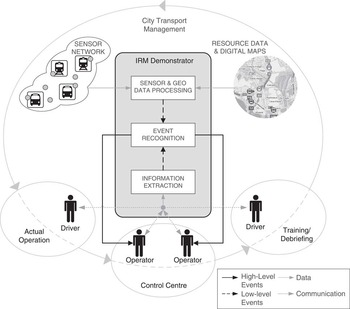
To illustrate the reviewed approaches we will use a real-world case study: event recognition for city transport management (CTM). In the context of the PRONTO projectFootnote 3, an event recognition system is being developed with the aim to support the management of public transport—see Figure 1. Buses and trams are equipped with in-vehicle units that send GPS coordinates to a central server, offering information about the current status of the transport system (e.g. the location of buses and trams on the city map). Additionally, buses and trams are being equipped with sensors for in-vehicle temperature, in-vehicle noise level and acceleration. Given the LLE that will be extracted from these sensors and other data sources, such as digital maps, as well as LLE that will be extracted from the communication between the drivers and the public transport control centre, HLE will be recognized related to, among others, the punctuality of a vehicle, passenger and driver comfort, passenger and driver safety and passenger satisfaction. A detailed description of this case study may be found in Artikis et al. (Reference Artikis, Kukurikos, Paliouras, Karampiperis and Spyropoulos2011).
Event Recognition for City Transport Management. IRM = Intelligence Resource Management

2 Chronicle recognition
Chronicle recognition systems are temporal reasoning systems developed for efficient, run-time HLE—chronicle—recognition. A chronicle is expressed in terms of a set of events linked together by time constraints and, possibly, a set of context constraints. A number of implementations have been developed for chronicle recognition. In this section, we will present the CRS of Dousson and colleaguesFootnote 4 (Dousson, Reference Dousson2002; Dousson & Maigat, Reference Dousson and Maigat2006, Reference Dousson and Maigat2007). CRS is an extension of IxTeT (Ghallab & Alaoui, Reference Ghallab and Alaoui1989; Dousson et al., Reference Dousson, Gaborit and Ghallab1993; Dousson, Reference Dousson1996; Ghallab, Reference Ghallab1996), a version of which was marketed and tested for the supervision of gas turbines, aircraft turbines and electrical power networks. CRS has been applied to numerous application domains such as cardiac monitoring (Callens et al., Reference Callens, Carrault, Cordier, Fromont, Portet and Quiniou2008), intrusion detection (Morin & Debar, Reference Morin and Debar2003) and mobility management (Dousson et al., Reference Dousson, Pentikousis, Sutinen and Mäkelä2007) in computer networks and distributed diagnosis of web services (Le Guillou et al., Reference Le Guillou, Cordier, Robin and Rozé2008).
In the following section, we present the input language of CRS; in Section 2.2 we present various reasoning algorithms of this system; and in Section 2.3 we present techniques for automatically constructing HLE definitions in the CRS language.
2.1 Representation
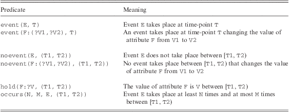
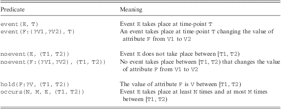
A chronicle can be seen as a HLE—as mentioned above, it is expressed in terms of a set of events linked together by time constraints and, possibly, a set of context constraints. The input language of CRS relies on a reified temporal logic, where propositional terms are related to time-points or other propositional terms. Time is considered as a linearly ordered discrete set of instants. The language includes predicates for persistence, event absence and event repetition. Table 1 presents the CRS predicates. Variables start with an upper case letter, while predicates and constants start with a lower-case letter. ? is the prefix of an atemporal variable. ‘Attributes’ represent context information. Attributes and events (also called ‘messages’ in the CRS language) may have any number of parameters. Details about the input language of CRS, and CRS in general, can be found on the web page of the system (see footnote 4).
Predicates of the Chronicle Recognition System
The code below, for example, expresses HLE related to vehicle (bus/tram) punctuality in the CRS language:
(1) chronicle punctual [?Id, ?VehicleType] (T2) {
(2) event (stop_enter [?Id, ?VehicleType, ?StopId, scheduled], T1)
(3) event (stop_leave [?Id, ?VehicleType, ?StopId, scheduled], T2)
(4) T2−T1 in [1, 2000]
(5) }
(6) chronicle non_punctual [?Id, ?VehicleType] (T1) {
(7) event (stop_enter [?Id, ?VehicleType, *, late], T1)
(8) }
(9) chronicle punctuality_change [?Id, ?VehicleType, non_punctual] (T2) {
(10) event (punctual[?Id, ?VehicleType], T1)
(11) event (non_punctual [?Id, ?VehicleType], T2)
(12) T2−T1 in [1, 20000]
(13) noevent (punctual [?Id, ?VehicleType], (T1+1, T2))
(14) noevent(non_punctual [?Id, ?VehicleType], (T1+1, T2))
(15) }
The atemporal variables of a chronicle (HLE) and an event (LLE or HLE) are displayed in square brackets. * denotes that a variable can take any value. Lines (1)–(5) of the above CRS code express a set of conditions in which a vehicle of a particular type (represented by VehicleType) and Id is said to be punctual: the vehicle enters a stop and leaves the same stop (represented by StopId) at the scheduled time. The time-stamp of the ‘punctual’ HLE is the same as that of the ‘stop leave’ sub-event (i.e. T2). The first and the last sub-event of the ‘punctual’ HLE, that is, ‘stop enter’ and ‘stop leave’, must take place within 2000 time-points in order to recognize ‘punctual’ (see Line (4)). Lines (6)–(8) express one out of several cases in which a vehicle is said to be non-punctual: the vehicle enters a stop after the scheduled time (i.e. it is late). ‘Non-punctual’ (respectively ‘punctual’) is defined as a disjunction of ‘stop enter’ and ‘stop leave’ LLE satisfying certain conditions. Disjunction is expressed in the CRS language with the use of multiple chronicles (explicit representation of disjunction is not allowed because it makes reasoning in CRS NP-complete—a presentation of the reasoning techniques of CRS is given in the following section). For simplicity, we do not show here the chronicles expressing the other cases in which a vehicle is said to be non-punctual (respectively, punctual).
Lines (9)–(15) of the above code fragment express the ‘punctuality change’ HLE: punctuality changes (to non-punctual) when a vehicle that was punctual at an earlier time now is not punctual. Another HLE definition (similar to the one shown above) deals with the case in which a vehicle was not punctual earlier and now is punctual.
Both quantitative and qualitative temporal constraints can be represented in the CRS language, the latter being replaced by numerical constraints during compilation—for instance, a constraint of the form T1 > T0 is translated to T1−T0 in [1, ∞). More details about the compilation stage of CRS are given in the following section. Note that the CRS language allows events not to be completely ordered. Consider the following code fragment:
event (abrupt_acceleration [?Id, ?VehicleType], T1)
event(sharp_turn [?Id, ?VehicleType], T2)
T2−T1 in [−3, 8]
According to the above constraints, ‘sharp turn’ may take place before, at the same time or after ‘abrupt acceleration’.
All events shown in the above code fragments are instantaneous. CRS does not allow for the explicit representation of durative events. One may implicitly represent the interval/duration of such an event in the CRS language by representing two instantaneous events, one indicating the time-point at which the durative event starts taking place, and one indicating the time-point at which it stops occurring. The CRS treatment of durative events allows the representation of the interval relations of a restricted interval algebra (Vilain and Kautz, Reference Vilain and Kautz1986; Nebel and Bürckert, Reference Nebel and Bürckert1995), but does not support all of Allen's (Reference Allen1983) interval relations.
Often in the literature, durative events are not even implicitly represented—they are treated as if they occur at an atomic instant. It has been pointed out (Paschke, Reference Paschke2005) that such a treatment leads to logical problems and unintended semantics for several event algebra operators—such operators facilitate the development of HLE definitions.
CRS is a temporal reasoner and, as such, it does not support mathematical operators on the constraints of atemporal variables. It is not possible to compute the distance between two entities given their coordinates, for example. In the CTM HLE definition concerning passenger safety, for instance, we cannot express that a vehicle accident or violence within a vehicle is more severe when the vehicle is far from a hospital or a police station. Moreover, the CRS language does not support universally quantified conditions. In CTM, for instance, we cannot define HLE using LLE coming from all vehicles (of a particular route).
Although the CRS language is limited in the aforementioned ways, it has proven to be expressive enough for numerous application domains, some of which were mentioned in the beginning of Section 2.
2.2 Reasoning
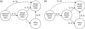
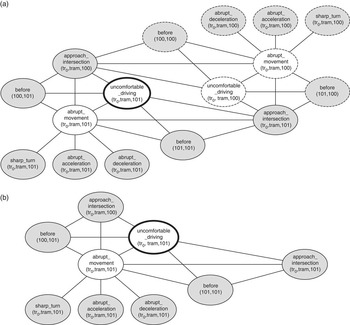
Each HLE definition expressed in the CRS language is typically translated to a Temporal Constraint Network (TCN; Dechter et al., Reference Dechter, Meiri and Pearl1991; Dousson, Reference Dousson1996; Ghallab, Reference Ghallab1996; Dousson & Maigat, Reference Dousson and Maigat2007; see Choppy et al. (Reference Choppy, Bertrand and Carle2009), however, for a Petri-Net-based semantics of the CRS language). Each sub-event of a HLE definition corresponds to a node in the TCN, whereas the temporal constraints between two sub-events determine the edge between the nodes expressing the sub-events. Figure 2(a), for example, shows the TCN expressing the CTM HLE ‘uncomfortable driving’. The sub-events of this HLE are ‘approach intersection’, ‘abrupt deceleration’, ‘sharp turn’ and ‘abrupt acceleration’. The temporal constraints on these events that, if satisfied, will lead to the recognition of ‘uncomfortable driving’, are expressed by the edges of the TCN. For example, ‘abrupt deceleration’ should take place, at the earliest, 2 time-points after the ‘approach intersection’ LLE and, at the latest, 5 time-points after this LLE. Briefly, a vehicle is said to be driven in an uncomfortable manner if, within a specified time period, it approaches an intersection, and then decelerates abruptly, turns sharply and accelerates abruptly. (There are other ways of defining ‘uncomfortable driving’. This example is presented simply to provide a concrete illustration.) The CRS code of this simplified definition of ‘uncomfortable driving’ may be found below:
Temporal Constraint Network

(1) chronicle uncomfortable_driving [?Id, ?VehicleType] (T4) {
(2) event(approach_intersection [?Id, ?VehicleType], T1)
(3) event(abrupt_deceleration [?Id, ?VehicleType], T2)
(4) event(sharp_turn [?Id, ?VehicleType], T3)
(5) event(abrupt_acceleration [?Id, ?VehicleType], T4)
(6) T2 – T1 in [2, 5]
(7) T4 – T2 in [1, 5]
(8) T4 – T3 in [0, 8]
(9) T4 – T1 in [0, 10]
(10) T2 <= T3
(11) }
During the off-line compilation stage, CRS propagates the constraints of a TCN using an incremental path consistency algorithm (Mackworth & Freuder, Reference Mackworth and Freuder1985), in order to produce the least constrained TCN expressing the user constraints. Figure 2(b), for example, shows the TCN for ‘uncomfortable driving’ after constraint propagation. In this example, the edge between ‘abrupt deceleration’ and ‘sharp turn’, and that between ‘sharp turn’ and ‘abrupt acceleration’, becomes [0, 5] due to the temporal constraint [1, 5] between ‘abrupt deceleration’ and ‘abrupt acceleration’. The constraint [3, 10] (dashed in Figure 2(b)) is removed because it is redundant with respect to the two other constraints [2, 5] and [1, 5] from which it can be completely deduced.
The use of the incremental path consistency algorithm allows for checking the consistency of the temporal constraints of a TCN—see Dousson (Reference Dousson1996) for details. CRS, therefore, detects inconsistent HLE definitions at compile-time and reports the inconsistencies to the user.
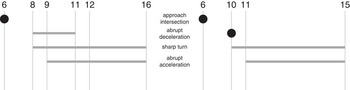
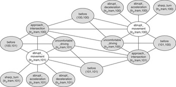
Once the least constrained TCNs expressing the user constraints have been compiled, HLE recognition may commence. The recognition process of CRS is illustrated in Figure 3—this figure shows the process of recognizing ‘uncomfortable driving’. The left part of Figure 3 shows the effects of the arrival of ‘approach intersection’ at time-point 6, while the right part of this figure shows the effects of the arrival of ‘abrupt deceleration’ at time-point 10. The arrival of ‘approach intersection’ creates an instance of ‘uncomfortable driving’, that is, a partial instantiation of the definition of this HLE. The horizontal grey lines in Figure 3 show the temporal windows of the sub-events of ‘uncomfortable driving’, that is, the possible times in which a sub-event may take place without violating the constraints of the ‘uncomfortable driving’ instance. Upon the arrival of ‘approach intersection’, the temporal window of ‘abrupt deceleration’ becomes [8, 11] because, according to the TCN of ‘uncomfortable driving’ (see Figure 2(b)), ‘abrupt deceleration’ must take place 2 time-points after the ‘approach intersection’ LLE at the earliest, and, at the latest, 5 time-points after this LLE. Similarly, the temporal window of ‘sharp turn’ becomes [8, 16], while that of ‘abrupt acceleration’ becomes [9, 16]. The occurrence of ‘abrupt deceleration’ at time-point 10 is integrated into the displayed instance of ‘uncomfortable driving’, as it complies with the constraints of the instance (i.e. ‘abrupt deceleration’ takes place within its temporal window), and constrains further the temporal windows of the (yet) undetected sub-events of ‘uncomfortable driving’ (see the right part of Figure 3).
High-Level Event Instance Recognition

Using this type of recognition, CRS may report to the user not only a fully recognized HLE, but also a partially recognized one, that is, a pending HLE instance. Moreover, CRS may report the events that need to be detected in order to fully recognize a HLE. These types of information have proven to be very helpful in various application domains (see, e.g. Gao et al., Reference Gao, Sripada, Hunter and Portet2009).
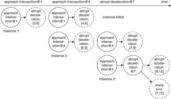
Figure 3 shows the evolution of one HLE instance. For each HLE definition more than one instance may be created. Figure 4 illustrates the instance management of CRS using the example of the ‘uncomfortable driving’ HLE. The occurrence of ‘approach intersection’ at time-point 1 creates a new instance of ‘uncomfortable driving’. CRS computes the temporal windows of the forthcoming events—for example, ‘abrupt deceleration’ is expected between [3, 6]. The occurrence of the second ‘approach intersection’ LLE at time-point 4 creates a new instance of ‘uncomfortable driving’. Moreover, the passing of time results in constraining the temporal windows of the forthcoming events of the first instance. For example, the temporal window of ‘abrupt deceleration’ becomes [4, 6]. Upon the arrival of ‘abrupt deceleration’ at time-point 7, CRS makes a copy of the second instance of ‘uncomfortable driving’, thus creating a third instance of this HLE, and integrates ‘abrupt deceleration’ into the third HLE instance. CRS keeps the second instance because another ‘abrupt deceleration’ LLE may take place in the future (more precisely, between 7 and 9), which may lead to another recognition of ‘uncomfortable driving’. The first instance of ‘uncomfortable driving’ is killed at time-point 7, because no ‘abrupt deceleration’ LLE was detected between [4, 6], and thus it is not possible to satisfy the constraints of this instance any more.
High-Level Event Instance Management

In the examples presented in this section, we assume that events arrive in a timely manner. Such an assumption is made to simplify the presentation. We will discuss shortly the consequences of the delayed arrival of events.
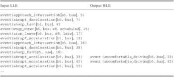
Table 2 illustrates event recognition in CRS using a larger LLE narrative. More precisely, this table shows an example LLE narrative concerning a particular vehicle, and the ‘uncomfortable driving’ HLE that are recognized given this narrative. By time-point 19, all sub-events of the ‘uncomfortable driving’ HLE are detected. However, this HLE is not recognized because the detected LLEs do not satisfy the temporal constraints of the HLE definition. The occurrence of ‘abrupt acceleration’ at time-point 19 is too late; at that time there are no pending instances of ‘uncomfortable driving’ (the last instance was killed at time-point 14).
Event Recognition in the Chronicle Recognition System

LLE = low-level events; HLE = high-level events.
The first recognition of ‘uncomfortable driving’ takes place at time-point 39. The occurrence of ‘abrupt acceleration’ at that time is integrated into the pending instance of ‘uncomfortable driving’ that consists of the occurrence of ‘approach intersection’ at time-point 36, ‘abrupt deceleration’ and ‘sharp turn’ at time-point 38. This instance is duplicated before integrating the occurrence of ‘abrupt acceleration’ at 39 because it may lead to another recognition of ‘uncomfortable driving’ in the future. Indeed, at time-point 42 ‘uncomfortable driving’ is recognized again: the occurrence of ‘abrupt acceleration’ at time-point 42 is integrated into the aforementioned pending instance.
Unlike the occurrences of ‘abrupt acceleration’ at time-points 39 and 42, the occurrence of this LLE at time-point 55 does not lead to the recognition of ‘uncomfortable driving’. At this time-point there is no pending instance of ‘uncomfortable driving’, as the last pending instance was killed at time-point 44.
CRS stores all pending HLE instances in trees, one for each HLE definition. At the arrival of a new event, and at a clock update, CRS traverses these trees in order to further develop, or kill, some HLE instances. For K HLE instances, each having n sub-events, the complexity of processing each incoming event or a clock update is  $ {\scr O}{\rm{(}}K{{n}^{\rm{2}}} {\rm{)}} $.
To allow for the delay in the information exchange between distributed components, such as the LLE detection component and the HLE recognition component, CRS processes LLEs arriving in a non-timely manner—the user specifies the maximum allowed delay for LLE. In this way, CRS may process LLEs arriving in a non-chronological order, that is, process LLEs that happened (were detected) before some of the already acquired LLEs. This feature, however, affects the efficiency of CRS: CRS delays the time at which a pending HLE instance must be killed due to the possibility of a late arrival of a sub-event of the HLE. In other words, the number K of HLE instances reduces at a slower rate.
Various techniques have been proposed for reducing the number K of HLE instances that are generated, and thus improving the efficiency of CRS. Bounding the temporal distance between the first sub-event and the last sub-event of a HLE (see, e.g. the definition of punctual in Section 2.1) is one way to reduce HLE instance duplication. Moreover, there may be HLEs that cannot have two completed instances overlapping in time or share the occurrence of an event. In this case, when a HLE instance is completed (the HLE is recognized) all its pending instances must be removed.
A recently developed technique for reducing the number of generated HLE instances, and, therefore, improving the efficiency of CRS, is called temporal focusing (Dousson & Maigat, Reference Dousson and Maigat2007). This technique can be briefly described as follows. Let us assume that, according to the definition of HLE Γ, event er should take place after event ef in order to recognize Γ, er is a very rare event and ef is a frequent event. The frequency of events is determined by an a priori analysis of the application under consideration. In this case, CRS stores all incoming ef events and starts the recognition process, that is, creates a new instance of Γ, only upon the arrival of an er event—the new instance will include er and a stored ef that satisfies the constraints of Γ. In this way the number of generated HLE instances is significantly reduced.
Temporal focusing significantly improves the efficiency of recognizing ‘uncomfortable driving’, for example, as ‘approach intersection’ is a very frequent LLE, ‘abrupt deceleration’ is a rare LLE, and ‘abrupt deceleration’ should take place after ‘approach intersection’ in order to recognize ‘uncomfortable driving’.
Empirical analysis has shown that CRS can be very efficient and scalable (Dousson & Maigat, Reference Dousson and Maigat2007).
Although the CRS language is fairly comprehensible, synthesizing and generalizing expert temporal knowledge, which can be highly application-dependent, is not a trivial task. Therefore, methods for automatically generating and refining HLE definitions from data are highly desirable. In the following section, we review machine learning techniques that have been used for constructing HLE definitions in the CRS language.
2.3 Machine learning
Various approaches have been proposed in the literature for the automated construction of HLE definitions expressed in the CRS language. One of the earliest approaches is the automata-based learning method of Ghallab (Reference Ghallab1996). Briefly, this method, which is inspired from learning techniques used in syntactical pattern recognition, learns automata from positive and negative HLE examples. Based on the learnt automata, discriminative ‘skeleton models’ are generated, containing only events and constraints, without context information. These skeleton models have to be completed by the human user with context information as well as quantitative temporal constraints.
Another line of research for the automated construction of HLE definitions concerns the use of unsupervised learning techniques. One such technique is the frequency-based analysis of sequences of events—see, for example, Dousson and Duong (Reference Dousson and Duong1999), Yoshida et al. (Reference Yoshida, Iizuka, Shiohara and Ishiguro2000), Fessant et al. (Reference Fessant, Clérot and Dousson2004); Hirate and Yamana (Reference Hirate and Yamana2006), Vautier et al. (Reference Vautier, Cordier and Quiniou2007) and Álvarez et al. (Reference Álvarez, Félix, Cariñena and Otero2010). Most of the approaches adopting this technique rely on an extended version of the Apriori algorithm (Mannila et al., Reference Mannila, Toivonen and Verkamo1997) to discover frequent sequences of events—the temporal distance between the events of a frequent sequence is computed using lower and higher frequency thresholds. A well-known approach for HLE definition discovery is the Frequency Analyser for Chronicle Extraction (FACE) system of Dousson and Duong (Reference Dousson and Duong1999). FACE uses an algorithm for incremental generation of definitions of HLE that are frequent in event narratives/logs. Fessant et al. (Reference Fessant, Clérot and Dousson2004) pointed out that FACE is very memory consuming in the presence of large event narratives. To address this issue, Fessant et al. proposed a pre-processing phase based on a Kohonen's self-organizing map (Kohonen, Reference Kohonen2001) to extract the most ‘interesting’ sub-narratives of events before the data mining phase of FACE. Frequency-based analysis is a promising approach for discovering unknown event patterns in databases or logs. However, these approaches are limited to propositional learning. Moreover, they may not be adapted to learning definitions of HLE that are not frequent in data—in some applications the recognition of such HLE is of utmost importance.
A common technique for learning HLE definitions in a supervised manner concerns the use of inductive logic programming (ILP; Muggleton, Reference Muggleton1991)—see, for example, Carrault et al. (Reference Carrault, Cordier, Quiniou and Wang2003) and Callens et al. (Reference Callens, Carrault, Cordier, Fromont, Portet and Quiniou2008). ILP is well suited to the construction of HLE definitions expressed in the CRS language because, among others, the CRS HLE definitions can be straightforwardly translated into the logic programming representation used by ILP systems and vice-versa—this translation is illustrated below. In what follows, therefore, we will present the use of ILP for constructing HLE definitions for CRS.
To illustrate the translation of CRS HLE definitions into logic programming consider, for example, the definition of ‘uncomfortable driving’ in logic programming (this definition was presented in the CRS language in the previous section):
uncomfortable_driving (T4, Id, VehicleType) ←
approach_intersection (T1, Id, VehicleType),
abrupt_deceleration (T2, Id, VehicleType),
sharp_turn (T3, Id, VehicleType),
abrupt_acceleration (T4, Id, VehicleType),
T2–T1 >= 2, T2–T1 =< 5,
T4–T2 >= 1, T4–T2 =< 5,
T4 >= T3, T4–T3 =< 8,
T4 >= T1, T4–T1 =< 10,
T2 =< T3
A chronicle (‘uncomfortable driving’, in this example), as well as every event in the definition of a chronicle (here ‘approach intersection’, ‘abrupt deceleration’, ‘sharp turn’ and ‘abrupt acceleration’), can be translated into a predicate whose arguments are the chronicle/event occurrence time (T1, for example) and the chronicle/event parameters (e.g. Id and VehicleType). Temporal constraints in the CRS language can be translated into arithmetic expressions—for instance, T2–T1 in [2, 5] can be translated into T2–T1 >= 2, T2–T1 =< 5. In general, any chronicle definition can be translated into a Horn clause whose head is the predicate representing the chronicle, and whose body is the conjunction of predicates representing the events of the chronicle and arithmetic expressions constraining the occurrence of these events.
ILP is the combination of inductive machine learning and logic programming. It aims at inducing theories from examples in the form of a first-order logic program. It inherits, from machine learning, the principle of hypothesis induction from data, but its first-order logic representation allows the induction of more expressive theories than classical machine learning approaches, which induce propositional hypotheses. Furthermore, a priori background knowledge, such as human expertise, can easily be used to guide learning. ILP has proven adequate in learning from very small data sets, especially in the presence of strong prior knowledge, while making good use of large volumes of data, where available. This also includes constructing theories that capture exceptional cases in data sets, where exceptions are a small minority of a data set. A detailed account of ILP may be found in Dzeroski and Lavrac (Reference Dzeroski and Lavrac2001) and Konstantopoulos et al. (Reference Konstantopoulos, Camacho, Fonseca and Costa2008), for example.
The logical elements involved in ILP can be defined as follows:
• A set of positive examples E + and a set of negative examples E −. These are typically ground facts.
• A hypothesis language
 $ {{{\scr L}}_H} $, from which hypotheses H are constructed.
• A background knowledge base B. B and H are sets of clauses/rules of the form α ← l1, …, ln where α is a ‘head’ literal and each li is a ‘body’ literal.

ILP searches for hypotheses  $ H\: \subseteq \:{{{\scr L}}_H} $, such that
 $ B\: \wedge \:H\: \models \:{{E}^ + } $ (completeness) and
 $ B\: \wedge \:H\: \wedge \:{{E}^{\rm{ - }}} $ ⊭□ (consistency; Muggleton & Raedt, Reference Muggleton and Raedt1994). The completeness condition guarantees that all positive examples in E + can be deduced from H and B. The consistency condition guarantees that no negative example in E − can be deduced from H and B.
Different ILP methods adopt different strategies to induce hypotheses H. A simple and common approach starts by selecting a positive example e + from E +, constructing a conjunctive first-order clause  $ h\: \in \:{{{\scr L}}_H} $ that entails e +, with respect to the background knowledge B, but does not entail any example from E −. All positive examples covered by h are then removed and the same procedure is iterated over the remaining positive examples to produce a new clause. Learning a clause h can be seen as walking through the space of clauses of
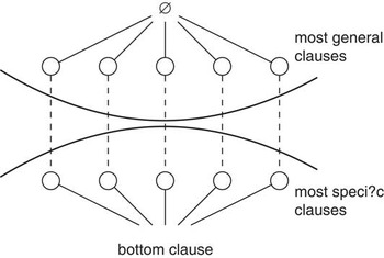
 $ {{{\scr L}}_H} $ that entail e +, with respect to B. Such a space, also known as version space, is shown in Figure 5. The empty clause, that is, the most general clause, is at the top of the space, and the most specific clause from
 $ {{{\scr L}}_H} $ that entails e + with respect to B—the ‘bottom clause’—is at the bottom of the space. According to the strategy that is adopted, the search may be general-to-specific or specific-to-general. In a general-to-specific strategy, the search will start with the empty clause and will try to specialize it, for instance, by adding conjuncts that cover the positive example and help exclude negative ones. The opposite happens in a specific-to-general strategy that starts with the bottom clause. An exhaustive search is usually impossible, due to the exponential complexity of the version space, and thus pruning and heuristics must be used to guide the search. For instance, during the search, if a clause does not cover the positive example under consideration (respectively, covers a negative example), then it is meaningless to specialize (generalize, respectively) this clause further because it would not improve its coverage. When using a search method that allows backtracking, such as best-first search, a small list of the ‘best’ clauses generated so far is maintained, sorted according to their coverage. In this manner, search can backtrack directly to the next best option and continue from that point in the version space.
Version Space

Reducing the version space and guiding more efficiently the search are two of the main challenges of ILP. One way to address these challenges is by acting on inductive bias. In ILP, three types of bias are used (Nédellec et al., Reference Nédellec, Rouveirol, Adé, Bergadano and Tausend1996): the search bias, which specifies how the space is walked; the validation bias, which determines the criteria according to which a candidate hypothesis (clause) is evaluated; and the language bias, which restricts  $ {{{\scr L}}_H} $. A form of language bias that is typically used in ILP is called mode declarations. This particular form of bias will be illustrated presently.
Many ILP algorithms have been developed in the literature. These algorithms differ in, among others, the way they perform the search, and the way they bias learning. Examples of ILP algorithms include First-order Inductive Learner (FOIL) (Quinlan & Cameron-Jones, Reference Quinlan and Cameron-Jones1995), ProgolFootnote 5 (Muggleton & Bryant, Reference Muggleton and Bryant2000), Inductive Classification Logic (icl)Footnote 6 (Laer, Reference Laer2002) and A Learning Engine for Proposing Hypotheses (Aleph)Footnote 7. In what follows, we illustrate the use of Aleph—a frequently used ILP algorithm—for learning HLE definitions expressed in the CRS language. A detailed example of learning CRS HLE definitions using ILP may be found in (Carrault et al., Reference Carrault, Cordier, Quiniou and Wang2003).
To learn hypotheses H expressing HLE definitions of ‘uncomfortable driving’, for example, we use the following background knowledge B (only a fragment of B is shown here):
% LLE for bus b1
stop_enter(e1, init, pos1, 0, b1, bus, s8, scheduled)
stop_leave(e2, e1, pos1, 1, b1, bus, s8, late)
approach_intersection(e3, e2, pos1, 2, b1, bus)
abrupt_deceleration(e4, e3, pos1, 4, b1, bus)
sharp_turn(e5, e4, pos1, 6, b1, bus)
abrupt_acceleration(e6, e5, pos1, 8, b1, bus)
…
quantitative_distance(e2, e1, 1)
quantitative_distance(e3, e2, 1)
quantitative_distance(e4, e3, 2)
quantitative_distance(e5, e4, 2)
quantitative_distance(e6, e5, 2)
…
% domain_knowledge
qualitative_distance(X, Y, very_long) ←
quantitative_distance(X, Y, D),
D>120
qualitative_distance(X, Y, long) ←
quantitative_distance(X, Y, D),
D>10, D<121
qualitative_distance(X, Y, short) ←
quantitative_distance(X, Y, D),
D>5, D<11
qualitative_distance(X, Y, very_short) ←
quantitative_distance(X, Y, D),
D<6
B includes the event narrative used for learning the hypotheses and a set of rules expressing domain knowledge. In this example, the narrative consists of a stream of detected CTM LLE. Each predicate representing a LLE, such as approach_intersection, has the following arguments: the first argument represents the id of the LLE, while the second argument represents the id of the directly temporally preceding LLE. init that there is no temporally preceding LLE, that is, the LLE having init as the second argument is the first LLE of the sequence. The first two arguments of LLE specify event chaining in a symbolic manner. Such a symbolic representation of temporal relations between events is necessary because Aleph does not perform numerical reasoning. The third argument of a LLE predicate associates the LLE with a positive example from E + (such as the first positive example pos1) or a negative example from E −, while the fourth argument represents the occurrence time of the LLE. The remaining arguments represent the standard properties of the LLE.
The quantitative_distance facts included in B express the temporal distance between two events. The qualitative_distance rules express domain knowledge: they translate the numerical temporal distances into symbolic distances (for example, 2 becomes very_short). This translation is necessary because, as mentioned earlier, Aleph does not perform numerical reasoning. The distance classification may be obtained by simple equal-frequency discretization on a log of quantitative_distance facts, or by expertise if available.
Apart from the background knowledge B, we specify a set of mode declarations M—a type of language bias—to restrict the version space. Consider the following declarations specified for learning the definition of ‘uncomfortable driving’:
:- modeh (1,uncomfortable_driving(+ex))
:- modeb(1,stop_enter(−event,−event,+ex,−int,−id,−vehicletype,−stopid, −timetablecompliance))
:- modeb(1,stop_leave(−event,−event,+ex,−int,−id,−vehicletype,−stopid, −timetablecompliance))
:- modeb(1,approach_intersection(−event,−event,+ex,−int,−id,−vehicletype))
:- modeb(1,abrupt_deceleration(−event,−event,+ex,−int,−id,−vehicletype))
:- modeb(1,sharp_turn(−event,−event,+ex,−int,−id,−vehicletype))
:- modeb(1,abrupt_acceleration(−event,−event,+ex,−int,−id,−vehicletype))
:- modeb(*,qualitative_distance(+event,+event,#duration))
A mode declaration is either a head declaration modeh(r, s) or a body declaration modeb(r, s), where s is a ground literal, the ‘scheme’, which serves as a template for literals in the head or body of a hypothesis clause, and r is an integer, the ‘recall’, which limits how often the scheme is used. An asterisk * denotes an arbitrary recall. The placemarkers +, −, # express, respectively, input terms, output terms and ground terms. Any input term in a body literal must be an input term in the head or an output term in some preceding body literal. A set M of mode declarations defines a language  $ {\scr L}{\rm{(}}M{\rm{)}}\: \subseteq \:{{{\scr L}}_H} $ within which a hypothesis H must fall, that is,
 $ H\: \subseteq \:{\scr L}{\rm{(}}M{\rm{)}} $. A clause α ← l 1, …, ln belongs in
 $ {\scr L}(M) $ if and only if the head literal α (respectively each body literal li) is obtained from some head (respectively body) declaration in M by replacing all # placemarkers with ground terms, all + placemarkers with input variables, and all—placemarkers with output variables. Given that
 $ H\: \subseteq \:{\scr L}{\rm{(}}M{\rm{)}} $, the head of a hypothesis, in the presented illustration, is uncomfortable_driving, while in the body of a hypothesis we may have a predicate expressing the LLE shown above, as well as qualitative_distance expressing the temporal distance between these LLE. No other LLE may be in the body of uncomfortable_driving (we set this constraint due to prior knowledge about the sub-events of uncomfortable_driving).
Other types of bias may also be used, such as setting the maximum number of body literals that a clause may contain.
Finally, to further guide the learning, we have set the following ‘integrity constraint’:
⊥ ← hypothesis(-, Body, -),
broken_sequence(Body)
hypothesis is a built-in Aleph predicate—the second argument of this predicate expresses the body of the hypothesis clause currently under consideration. broken_sequence(Body) is a user-defined predicate that is true when more than one literal (event) in the Body does not have its directly temporally preceding event in Body. The above integrity constraint, therefore, states that any candidate hypothesis clause in which there is more than one event in the body that does not have a directly temporally preceding event must be discarded. The absence of a temporally preceding event is allowed only for the initial event of a hypothesis clause.
To learn a hypothesis H concerning uncomfortable_driving, a set of positive examples E + and a set of negative examples E − are given:
% E+
uncomfortable_driving(pos1)
…
% E+
uncomfortable_driving(neg1)
…
Using the background knowledge B, various types of bias, integrity constraints, positive examples E + and negative examples E −, Aleph performs the following operations. First, it selects an example from E + to be generalized (such as uncomfortable_driving(pos1)). Second, it generates the most specific clause that entails this example with respect to B. In the case of uncomfortable_driving(pos1) the following clause is produced:
[bottom clause]
uncomfortable_driving(Ex) ←
stop_enter(E1, Init, Ex, T1, Id, VehicleType, StopId, TC1),
stop_leave(E2, E1, Ex, T2, Id, VehicleType, StopId, TC2),
approach_intersection(E3, E2, Ex, T3, Id, VehicleType),
abrupt_deceleration(E4, E3, Ex, T4, Id, VehicleType),
sharp_turn(E5, E4, Ex, T5, Id, VehicleType),
abrupt_acceleration(E6, E5, Ex, T6, Id, VehicleType),
qualitative_distance(E2, E1, very short),
qualitative_distance(E3, E2, very short),
qualitative_distance(E4, E3, very short),
qualitative distance(E5, E4, very short),
qualitative_distance(E6, E5, very short)
Third, Aleph searches for a more general clause than that generated in the previous step, aiming to cover as many positive examples from E + as possible, without covering any negative examples from E −. Fourth, it adds the clause to H, removing redundant clauses and restarting with a new example from E + until E + is empty.
In practice, the examples used to induce a hypothesis H, as well as the event narrative that is part of B, may be noisy. In order to facilitate learning under such conditions, ILP systems relax the consistency and completeness requirements, allowing some negative examples to be deduced from H and B and some positive ones to not be covered. An approach that has been specifically developed for learning hypotheses in noisy environments is presented in Section 4.
The result of ILP, in this case, comprises the following:
[Rule 1]
uncomfortable_driving(Ex) ←
approach_intersection(E1, Init, Ex, T1, Id, VehicleType),
abrupt_deceleration(E2, E1, Ex, T2, Id, VehicleType),
sharp_turn(E3, E2, Ex, T3, Id, VehicleType),
abrupt_acceleration(E4, E3, Ex, T4, Id, VehicleType),
qualitative_distance(E2, E1, very short),
qualitative_distance(E3, E2, very short),
qualitative_distance(E4, E3, very short)
The above clause is translated into the following CRS code:
chronicle uncomfortable_driving [?Id, ?VehicleType](T4) {
event(approach_intersection [?Id, ?VehicleType], T1)
event(abrupt_deceleration [?Id, ?VehicleType], T2)
event(sharp_turn [?Id, ?VehicleType], T3)
event(abrupt_acceleration [?Id, ?VehicleType], T4)
T2 – T1 in [0, 5]
T3 – T2 in [0, 5]
T4 – T3 in [0, 5]
}
The above CRS code represents a less accurate account of the numerical temporal constraints than that of the definition presented in Section 2.2, but the HLE structure has been correctly discovered, without adding any unnecessary sub-events such as stop_leave. Learning numerical temporal constraints with the use of ILP is an issue of current research.
Learning HLE definitions that have other HLE as sub-events is performed in a similar manner. In this case, however, one would have to add to the background knowledge base B a HLE narrative, as opposed to a LLE narrative. To learn the definition of the punctuality_change HLE, for example, B would have to include a narrative of punctual and non-punctual HLE.
3 The Event Calculus
The EC was introduced by Kowalski and Sergot (Reference Kowalski and Sergot1986) as a logic programming framework for representing and reasoning about events and their effects. Since then various alternative formalizations and implementations have been developed. As Miller and Shanahan (Reference Miller and Shanahan2002) point out, EC has been reformulated in various logic programming forms (for instance, Sadri & Kowalski, Reference Sadri and Kowalski1995; Chittaro & Montanari, Reference Chittaro and Montanari1996; Denecker et al., Reference Denecker, Belleghem, Duchatelet, Piessens and Schreye1996; Paschke, Reference Paschke2005), in classical logic (e.g. Miller & Shanahan, Reference Miller and Shanahan1999; Shanahan, Reference Shanahan1999; Cervesato et al., Reference Cervesato, Franceschet and Montanari2000; Mueller, Reference Mueller2006a), in modal logic (e.g. Cervesato et al., Reference Cervesato, Franceschet and Montanari1997, Reference Cervesato, Franceschet and Montanari1998, Reference Cervesato, Franceschet and Montanari2000), and even in non-logic-based languages (such as Farrell et al., Reference Farrell, Sergot, Sallé and Bartolini2005).
EC has been frequently used for event recognition—to the best of our knowledge, only in a logic programming form, as in Chittaro and Dojat (Reference Chittaro and Dojat1997), Cervesato and Montanari (Reference Cervesato and Montanari2000), Chaudet (Reference Chaudet2006), Paschke (Reference Paschke2005, Reference Paschke2006), Paschke et al. (Reference Paschke, Kozlenkov and Boley2007), Paschke and Bichler (Reference Paschke and Bichler2008), Teymourian and Paschke (Reference Teymourian and Paschke2009) and Artikis et al. (Reference Artikis, Sergot and Paliouras2010b, Reference Artikis, Kukurikos, Paliouras, Karampiperis and Spyropoulos2011).
EC is related to other formalisms proposed in the literature of commonsense reasoning, such as the Situation Calculus (McCarthy and Hayes, Reference McCarthy and Hayes1969; Reiter, Reference Reiter2001), the action language C+ (Akman et al., Reference Akman, Erdogan, Lee, Lifschitz and Turner2004; Giunchiglia et al., Reference Giunchiglia, Lee, Lifschitz, McCain and Turner2004), the fluent calculus (Thielscher, Reference Thielscher1999, Reference Thielscher2001) and Temporal Action Logics (Doherty et al., Reference Doherty, Gustafsson, Karlsson and Kvarnström1998; Kvarnström, Reference Kvarnström2005). Comparisons between formalisms for commonsense reasoning and proofs of equivalence between some of them may be found in Kowalski and Sadri (Reference Kowalski and Sadri1997), Miller and Shanahan (Reference Miller and Shanahan2002), Mueller (Reference Mueller2006a, Reference Mueller2006b), and Craven (Reference Craven2006), for example. The advantages of EC over other formalisms for commonsense reasoning with respect to event recognition are outlined in Paschke (Reference Paschke2005) and Paschke and Kozlenkov (Reference Paschke and Kozlenkov2009).
In the following section, we present a high-level review of the expressiveness of EC as a logic programming language, in Section 3.2 we present a concrete implementation of this formalism, while in Section 3.3 we present techniques for automatically constructing and refining an EC logic program.
3.1 Representation
In this section, we present features of typical EC dialects for event recognition (Cervesato & Montanari, Reference Cervesato and Montanari2000; Paschke, Reference Paschke2005; Artikis et al., Reference Artikis, Sergot and Paliouras2010b). The time model of EC is often linear and it may include real numbers or integers. Where F is a fluent—a property that is allowed to have different values at different points in time—the term F = V denotes that fluent F has value V. Boolean fluents are a special case in which the possible values are true and false. Informally, F = V holds at a particular time-point if F = V has been initiated by an event at some earlier time-point, and not terminated by another event in the meantime.
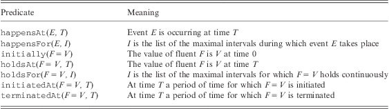
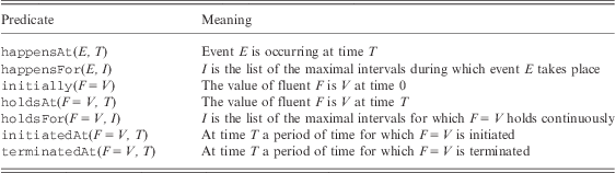
An event description in EC includes rules that define the event occurrences, the effects of events and the values of fluents. Table 3 presents typical predicates of EC dialects for event recognition. Variables start with an upper-case letter while predicates and constants start with a lower-case letter.
Main Predicates of the Event Calculus
An EC dialect for event recognition has typically built-in rules for holdsAt and holdsFor, that is, for computing the value of a fluent at a particular time and for computing the maximal intervals in which a fluent has a particular value (there are EC dialects with additional built-in rules for more expressive temporal representation (Miller & Shanahan, Reference Miller and Shanahan2002)). A partial specification of holdsAt, for example, is given below:
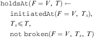 $$ \matrix { {{\rm{\tf="courier" holdsAt}}(F\: = \:V,\;T) \leftarrow } \hfill \cr\ {\; \; \; \; {\rm{\tf="courier" initiatedAt}}(F\: = \:V,\;{{T}_s}),} \hfill \cr\ {\; \; \; \; {{T}_s}\:{\leqslant}\:T,} \hfill \cr\ {\; \; \; \; {\rm{\tf="courier" not}}\;{\rm{\tf="courier" broken}}(F\: = \:V,\;{{T}_s},\;T)} \hfill \\\end{} $$
 $$\matrix { {{\rm{\tf="courier" broken}}(F\: = \:V,\;{{T}_s},\;T) \leftarrow } \hfill \cr\ {\; \; \; \; {\rm{\tf="courier" terminatedAt}}(F\: = \:V,\;{{T}_e}),} \hfill \cr\ {\; \; \; \; {{T}_s}\:{\leqslant}\:{{T}_e}\:{\leqslant}\:T} \hfill \\\end{}$$
not represents ‘negation by failure’ (Clark, Reference Clark1978). The above rules state that F = V holds at T if F = V has been initiated at Ts, where Ts ⩽ T, and not ‘broken’, that is, terminated in the meantime. The events that initiate/terminate a fluent are represented in the body of initiatedAt and terminatedAt—the definitions of these two predicates are specific to the domain under consideration.
Alternatively, holdsAt may be defined in terms of holdsFor:
 $$ \matrix { {{\rm{\tf="courier" holdsAt}}(F\: = \:V,\;T) \leftarrow } \hfill \cr\ {\; \; \; \; {\rm{\tf="courier" holdsFor}}(F\: = \:V,\;I),} \hfill \cr\ {\; \; \; \; ({{T}_s},{{T}_e})\: \in \:I,} \hfill \cr\ {\; \; \; \; {{T}_s}\:{\leqslant}\:T\: \lt \:{{T}_e}} \hfill \\\end{} $$
For any fluent F, holdsAt(F = V, T) if and only if time-point T belongs to one of the maximal intervals of I such that holdsFor(F = V, I). Intervals (Ts, Te) in the presented EC representation correspond to [Ts, Te). Quite elaborate implementations of holdsFor have been proposed in the literature. In the following section, we sketch an implementation of holdsFor. For alternative implementations, the interested reader is referred to Cervesato and Montanari (Reference Cervesato and Montanari2000) and Artikis et al. (Reference Artikis, Sergot and Paliouras2010b).
To illustrate the use of EC for event recognition, below we present definitions of CTM HLE concerning vehicle (bus/tram) punctuality:
 $$\matrix { {{\rm{\tf="courier" happensAt\,(}}punctual{\rm{(}}Id{\rm{,}}\,VehicleType{\rm{),}}\;DT{\rm{)}} \leftarrow } \hfill \cr\ {\; \; \; \; {\rm{\tf="courier" happensAt\,(}}stop\_enter{\rm{(}}Id,\,VehicleType,\,StopId,scheduled{\rm{),}}\;AT{\rm{),}}} \hfill \cr\ {\; \; \; \; {\rm{\tf="courier" happensAt\,(}}stop\_leave{\rm{(}}Id{\rm{,}}\,VehicleType{\rm{,}}\,StopId{\rm{,}}\, scheduled{\rm{),}}\;DT{\rm{),}}} \hfill \cr\ {\; \; \; \; {\tf="Times-i" 1}\:{\leqslant}\:DT{\rm{ - }}AT\:{\leqslant}\:{\tf="Times-i" 2000}} \hfill \\\end{}$$
 $$\!\!\!\!\!\!\!\!\!\!\!\!\!\!\!\!\!\!\!\!\!\!\!\!\!\!\!\!\!\!\!\!\!\!\matrix { {{\rm{\tf="courier" happensAt\,(}}non\_punctual{\rm{(}}Id{\rm{,}}\,VehicleType{\rm{),}}\;AT{\rm{)}} \leftarrow } \hfill \cr\ {\; \; \; \; {\rm{\tf="courier" happensAt\,(}}stop\_enter{\rm{(}}Id{\rm{,}}\,VehicleType{\rm{,}}\,\_{\rm{,}}\,late{\rm{),}}\;AT{\rm{)}}} \hfill \\\end{}$$
According to the above formalization, a vehicle is said to be punctual if it enters and leaves a stop at the scheduled time. The LLE ‘stop enter’ and ‘stop leave’ must take place within 2000 time-points in order to recognize ‘punctual’. A vehicle is said to be non-punctual if it enters a stop later than the scheduled time. (These conditions are not the only ones in which a vehicle is said to be punctual/non-punctual.) All events in the above rules are instantaneous and thus they are represented by means of happensAt.
Punctuality change may be expressed in EC as follows:
 $$\!\!\!\!\!\!\!\!\!\!\!\!\!\!\!\!\!\!\!\!\!\!\!\!\!\!\!\!\!\!\!\!\!\!\!\!\!\!\!\!\!\!\!\!\!\!\!\!\!\!\!\!\!\!\!\matrix { {{\rm{\tf="courier" initially}}(punctuality(\_,\,\_)\: = \:punctual)} \hfill \\\end{}$$
 $$\matrix { {{\rm{\tf="courier" initiatedAt}}(punctuality(Id{\rm{,}}\,VehicleType)\: = \:punctual{\rm{,}}\;T) \leftarrow } \hfill \cr\ {\; \; \; \; {\rm{\tf="courier" happensAt}}(punctual(Id{\rm{,}}\,VehicleType){\rm{,}}\;T)} \hfill \\\end{}$$
 $$\ \ \quad\matrix { {{\rm{\tf="courier" initiatedAt}}(punctuality{\rm{(}}Id{\rm{,}}\,VehicleType{\rm{)}}\: = \:non\_punctual{\rm{,}}\;T) \leftarrow } \hfill \cr\ {\; \; \; \; {\rm{\tf="courier" happensAt}}(non\_punctual(Id{\rm{,}}\,VehicleType{\rm{),}}\;T)} \hfill \\\end{}$$
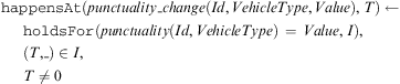 $$ \matrix { {{\rm{\tf="courier" happensAt(}}punctuality\_change{\rm{(}}Id{\rm{,}}\,VehicleType{\rm{,}}\,Value{\rm{),}}\;T) \leftarrow } \hfill \cr\ {\; \; \; \; {\rm{\tf="courier" holdsFor(}}punctuality{\rm{(}}Id{\rm{,}}\,VehicleType{\rm{)}}\, = \,Value{\rm{,}}\;I{\rm{)}},} \hfill \cr\ {\; \; \; \; {\rm{(}}T{\rm{,}}\_{\rm{)}}\: \in \:I{\rm{,}}} \hfill \cr\ {\; \; \; \; T\: \ne \:0} \hfill \\\end{} $$
We defined an auxiliary fluent, punctuality, that records the time-points in which a vehicle is (non-) punctual. The fluent punctuality is defined by rules (6)–(8). Initially, every vehicle is punctual. Thereafter, punctuality is affected by the punctual and non_punctual HLE. Rule (9) expresses the definition of the HLE punctuality_change. This rule uses the EC built-in implementation of holdsFor to compute the list of the maximal intervals for which a vehicle is continuously (non-)punctual. Punctuality changes at the first time-point of each of these intervals (see the last two lines of rule (9)).
Note that, depending on the requirements of the user (city transport officials, in the CTM example), punctuality may itself be a HLE, as opposed to an auxiliary construct. In general, a HLE may not necessarily be treated as an EC event. In some cases it is more convenient to treat a HLE as an EC fluent. In the case of a durative HLE Γ, for example, treating Γ as a fluent and using the built-in holdsFor to compute the intervals of Γ, may result in a more succinct representation than treating Γ as an EC event and developing domain-dependent rules for happensFor to compute the intervals of Γ.
Of interest to city transport officials are two HLEs concerning driving quality—these are defined as follows:
 $$\matrix{ {{\rm{\tf="courier" happensFor}}(medium\_quality\_driving(Id{\rm{,}}\,VehicleType{\rm{),}}\;MQDI) \leftarrow } \hfill \cr\ {\; \; \; \; {\rm{\tf="courier" happensFor}}(uncomfortable\_driving(Id{\rm{,}}\,VehicleType{\rm{),}}\;UCI),} \hfill \cr\ {\; \; \; \; {\rm{\tf="courier" holdsFor}}(punctuality(Id{\rm{,}}\ VehicleType{\rm{)}}\: = \:punctual{\rm{,}}\;PunctualI),} \hfill \cr\ {\; \; \; \; {\rm{\tf="courier" intersect\_all}}({\rm{[}}UCI{\rm{,}}\ \:PunctualI{\rm{],}}\;MQDI{\rm{)}}} \hfill \\\end{}$$
 $$\matrix { {{\rm{\tf="courier" happensFor}}(low\_quality\_driving{\rm{(}}Id{\rm{,}}\ VehicleType{\rm{),}}\;LQDI) \leftarrow } \hfill \cr\ {\; \; \; \; {\rm{\tf="courier" happensFor}}(unsafe\_driving{\rm{(}}Id{\rm{,}}\ VehicleType{\rm{),}}\;USI),} \hfill \cr\ {\; \; \; \; {\rm{\tf="courier" holdsFor}}(punctuality{\rm{(}}Id{\rm{,}}\ VehicleType{\rm{)}}\: = \:non\_punctual{\rm{,}}\;NPI),} \hfill \cr\ {\; \; \; \; {\rm{\tf="courier" union\_all([}}USI{\rm{,}}\ NPI{\rm{],}}\;LQDI{\rm{)}}} \hfill \\\end{}$$
happensFor represents the list of the maximal intervals during which an event takes place (see Table 3). Note that in the case where an event E has not taken place, we have happensFor (E, []). Similarly, if F = V is never the case, we have holdsFor (F = V, []). intersect_all computes the intersection of a list of lists of maximal intervals. For example, intersect_all ([[(5, 20), (26, 30)], [(28, 35)]], [(28, 30)]). Similarly, union_all computes the union of a list of lists of maximal intervals. For example, union_all ([[(5, 20), (26, 30)], [], [(28, 35)]], [(5, 20), (26, 35)]). Medium quality driving is recognized when the driving style is uncomfortable, but the vehicle is punctual. Low quality driving is recognized when the driving style is unsafe or the vehicle is non-punctual. punctuality is defined by rules (6)–(8). To simplify the presentation we do not show here the definitions of the uncofmortable_driving and unsafe_driving HLE (see Artikis et al., Reference Artikis, Kukurikos, Paliouras, Karampiperis and Spyropoulos2011) for an extensive library of CTM HLE definitions formalized in EC).
The use of interval manipulation constructs, such as union_all and intersect_all, often leads to a very concise HLE representation. Cervesato and Montanari (Reference Cervesato and Montanari2000) have used interval manipulation constructs in order to define a set of complex event operators in the context of EC. These operators are expressed as follows:
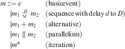 $$ \matrix { {m::\: = \:e} \hfill & {({\rm{basicevent}})} \hfill \cr\ {\; \; \; \; |{{m}_1}\ ;_{d}^{D} \;{{m}_2}} \hfill & {({\rm{sequence}}\,{\rm{with}}\,{\rm{delay}}\,d\,{\rm{to}}\,D)} \hfill \cr\ {\; \; \; \; |{{m}_1}\: + \:{{m}_2}} \hfill & {({\rm{alternative}})} \hfill \cr\ {\; \; \; \; |{{m}_1}\:\ ||\ \:{{m}_2}} \hfill & {({\rm{parallelism}})} \hfill \cr\ {\; \; \; \; |{{m}^\ast} } \hfill & {({\rm{iteration}})} \hfill \\\end{} $$
The semantics of the above event operators is given in terms of a predicate that computes the interval of a complex event given the intervals of its sub-events.
In a similar way, Paschke (Reference Paschke2005) has formalized the following event operators in the context of EC: sequence, disjunction, mutual exclusivity, conjunction, concurrency, negation, quantification and aperiodicity.
The availability of the full power of logic programming is one of the main attractions of using EC as the temporal formalism. It allows HLE definitions to include not only complex temporal constraints, but also complex atemporal constraints. For example, it is straightforward to develop in Prolog a predicate computing the distance between two entities.
The cited EC dialects for event recognition are not tied to a particular type of logic programming semantics. In this way, a dialect may be directly implemented in various existing rule languages (such as Prova).
Logic programming, not including an EC implementation, has been used frequently for event recognition. A notable example is the work of Shet and colleagues (Shet et al., Reference Shet, Harwood and Davis2005, Reference Shet, Harwood and Davis2006, Reference Shet, Neumann, Ramesh and Davis2007). A benefit of EC, in comparison with pure Prolog, is that EC has built-in rules for complex temporal representation, such as the ones presented here, which help considerably the development of HLE definitions.
3.2 Reasoning
Several implementations of the EC built-in rules have been proposed in the literature. Reasoning in EC is often performed at query-time, that is, the incoming LLE are logged without processing, and reasoning about the LLE log is performed when a query, concerning the recognition of HLE, is submitted. To perform run-time event recognition using query-time reasoning—to recognize, for example, at real-time incidents affecting the smooth operation of public transportation—one would have to repeatedly query EC (say every 5 seconds). If the outcome of query computation (the intervals of the recognized HLE) is not stored, reasoning would be performed on all detected LLE, as opposed to the LLE detected between two consecutive query times. Consequently, recognition time would substantially increase over time. (In retrospective recognition, such as the recognition performed at the end of each day in order to evaluate the performance of public transportation, querying about the intervals of a HLE is performed once, so there is considerably less need to store the outcome of query computation.)
To overcome the above limitation, a cached version of the EC has been proposed: the so-called Cached Event Calculus (CEC; Chittaro & Montanari, Reference Chittaro and Montanari1996). Reasoning in CEC is not performed at query-time, but at update-time: CEC infers and stores all consequences of LLE as soon as they arrive. Query processing, therefore, amounts to retrieving the appropriate HLE intervals from the memory. (Another EC dialect in which reasoning is performed at update-time may be found in Chesani et al. (Reference Chesani, Mello, Montali and Torroni2009). We do not discuss this dialect here because its reasoning efficiency has not been evaluated yet.)
Note that caching does not necessarily imply update-time reasoning. Caching techniques may be implemented for query-time reasoning.
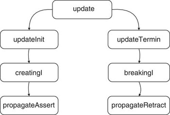
Figure 6 shows the main modules of CEC. Each new LLE is entered into the database using update. updateInit and updateTermin are then called to manage fluents that are initiated and, respectively, terminated by the LLE. A fluent may represent a HLE or it may represent a context variable used in the definition of a HLE. updateInit may call creatingI to create a new maximal interval for a fluent. updateTermin may call breakingI to break a maximal interval of a fluent. The modules propagateAssert and propagateRetract deal with the non-chronological arrival of LLE, that is, the arrival of a LLE that happened (was detected) before some of the already acquired LLE. When a maximal interval (or part of it) of a fluent is retracted, or asserted, as a result of the occurrence of a LLE that arrived in a non-chronological order, the update has to be propagated to the fluents whose validity may rely on such an interval. The retraction or assertion of an interval [T1, T2] in which a fluent has a particular value modifies the context of events occurring at time-points belonging to this interval, and possibly invalidates (or activates) the effects of these events. propagateAssert and propagateRetract may recursively activate the process of creating or breaking maximal intervals, by means of calling creatingI and breakingI. To avoid clutter in Figure 6, however, we do not show the information flow between propagateAssert, propagateRetract and the remaining CEC modules.
The Cached Event Calculus

We will illustrate the way CEC deals with the non-chronological arrival of LLE with the use of a simple example. Assume that we are interested in recognizing HLE related to vehicle punctuality (see rules (4)–(9)) and passenger satisfaction, a partial definition of which is presented below:
 $$\matrix{ {{\rm{\tf="courier" initiatedAt}}(reducing\_passenger\_satisfaction{\rm{(}}Id{\rm{,}}\,VehicleType{\rm{)}}\: = \:{\tf="courier" true}{\rm{,}}\;T) \leftarrow } \hfill \cr\ {\; \; \; \; {\rm{\tf="courier" happensAt}}(passenger\_density\_change{\rm{(}}Id{\rm{,}}\,VehicleType{\rm{,}}high{\rm{),}}\;T),} \hfill \cr\ {\; \; \; \; {\rm{\tf="courier" holdsAt}}(punctuality{\rm{(}}Id{\rm{,}}\,VehicleType{\rm{)}}\: = \:non\_punctual{\rm{,}}\;T)} \hfill \\\end{}$$
According to the above formalization, passenger satisfaction concerning a vehicle is said to be reducing when passenger density in that vehicle becomes high while the vehicle is non-punctual. Recall that, for any fluent F, holdsAt(F = V, T) if and only if time-point T belongs to one of the maximal intervals of I such that holdsFor(F = V, I)—see, for example, rule (3). Note that reducing_passenger_satisfaction, like punctuality, is represented as a fluent.
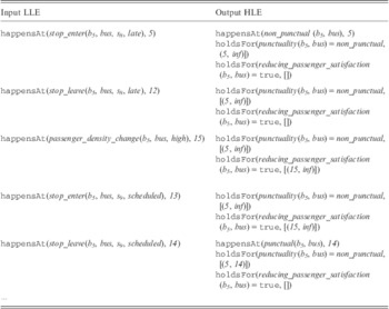
Table 4 shows an example LLE narrative concerning a particular vehicle and a set of HLE that are recognized given in this narrative—more precisely, Table 4 shows the instantaneous punctual and non_punctual HLE recognized at each time, the maximal intervals for which a vehicle is said to be non-punctual, and the durative reducing_passenger_satisfaction HLE. A maximal interval (Ts, inf) indicates that a fluent holds continuously since Ts. Moreover, as mentioned earlier, intervals (Ts, Te) in the presented EC representation correspond to [Ts, Te). Two LLE, in this example, arrive in a non-chronological order: stop_enter(b5, bus, s9, scheduled) and stop_leave(b5, bus, s9, scheduled). These LLEs happened (were detected) before one of the already acquired LLEs: passenger_density_change(b5, bus, high).
Event Recognition in the Cached Event Calculus

LLE = low-level events; HLE = high-level events.
Upon the arrival of the first LLE of the narrative displayed in Table 4, CEC recognizes that bus b5 is non-punctual. This is due to the fact that b5 entered stop s8 later than the scheduled time. Passenger satisfaction is not affected at this time—the list of the intervals for which passenger satisfaction is reducing remains empty. The arrival of the second LLE does not lead to the recognition of a new HLE. b5 is still considered non-punctual. The following LLE, passenger_density_change(b5, bus, high), leads to the recognition of reducing_passenger_satisfaction(b5, bus) because, at that time, bus b5 is considered non-punctual (see rule (12)). The next two LLEs arrive, as mentioned above, in a non-chronological order. They lead to the recognition of the punctual(b5, bus) HLE, which is said to take place at time-point 14 (see rule (4)). This HLE breaks the interval for which b5 is considered non-punctual. CEC, therefore, retracts the interval (14, inf) for which punctuality(b5, bus) = non_punctual.
Given that the retraction of the aforementioned fluent interval was due to LLE that arrived in a non-chronological order, CEC has to propagate the retraction to the fluents whose validity relies on this interval—in this example, to the fluent representing the ‘passenger satisfaction’ HLE (see rule (12)). The retraction of the interval (14, inf) for which punctuality(b5, bus) = non_punctual modifies the context of the passenger_density_change(b5, bus, high) LLE that happened at time-point 15—we now consider b5 punctual at that time-point. CEC, therefore, invalidates the effects of passenger_density_change(b5, bus, high): it retracts the interval (15, inf) for which reducing_passenger_satisfaction(b5, bus) = true.
The complexity of update processing (inferring and storing the consequences of an event) in CEC is measured in terms of accesses to happensAt and holdsFor Prolog facts, where happensAt facts represent the incoming LLE, while holdsFor facts represent cached fluent intervals, including HLE intervals. On this basis, the complexity of update processing in CEC, considering a particular fluent, is  $ {\scr O}{\rm{(}}{{n}^{({{L}_{fw}}\, + \,{\tf="Times-i" 1})\, + \,{\tf="Times-i" 2}}} {\rm{)}} $, where n is the number of initiating/terminating events for the fluent into consideration, and Lfw is the maximum number of propagations of fluent interval assertions and retractions—as shown above, such propagations are caused by LLEs arriving in a non-chronological order. Note that if Lfw = 0 then the complexity of update processing is
 $ {\scr O}{\rm{(}}{{n}^{\rm{2}}} {\rm{)}} $. The complexity of query processing (retrieving the cached maximal intervals of a fluent) in CEC is
 $ {\scr O}{\rm{(}}n{\rm{)}} $. Details about the complexity analysis of CEC may be found in Chittaro and Montanari (Reference Chittaro and Montanari1996).
The efficiency of CEC has been reported to be adequate for certain application domains (Chittaro & Dojat, Reference Chittaro and Dojat1997). In practice, where delayed LLEs are considered only if the delay does not exceed a certain threshold, the complexity of update processing is considerably less than the worst-case complexity presented above. Moreover, ways to improve the efficiency of CEC have been identified (Artikis et al., Reference Artikis, Kukurikos, Paliouras, Karampiperis and Spyropoulos2011). Note, however, that caching in CEC concerns only HLE represented as fluents, and thus needs to be extended to cater for HLE represented as EC events (such as, e.g. medium_quality_driving—see Section 3.1).
3.3 Machine learning
Since EC event descriptions are typically expressed as logic programs, ILP methods are an obvious candidate for constructing domain-dependent rules representing HLE definitions. As discussed in Section 2.3, ILP can be used to induce hypotheses from examples. For instance, to learn the definition of the HLE punctual, one has to provide positive examples E + and negative examples E − for punctual using the happensAt predicate, and a background knowledge base B including a LLE narrative. The learnt hypotheses will be of the form of rules (4) and (5). In general, learning hypotheses for predicates for which examples are available (such as happensAt(punctual(Id, VehicleType), T)), that is, ‘observation predicate learning’ (OPL; Muggleton & Bryant, Reference Muggleton and Bryant2000), may be achieved using ILP techniques as shown in Section 2.3.
Automatically constructing an EC logic program often includes learning hypotheses for predicates for which examples are not available, which implies that induction cannot be directly applied to produce the required hypotheses. Consider, for instance, the case in which we need to learn the definition of the CTM HLE ‘reducing passenger satisfaction’, we require to represent this HLE as a fluent in terms of initiatedAt (because, say, we expect that such a representation would be succinct), and the available examples for learning this HLE are given only in terms of holdsAt. In such a case, abduction may be combined with induction in order to produce the required hypotheses—a description of abductive logic programming may be found at Kakas et al. (Reference Kakas, Kowalski and Toni1992) and Denecker and Kakas (Reference Denecker and Kakas2000, Reference Denecker and Kakas2002), for example. Abduction may produce ground initiatedAt rules, using the examples expressed by means of holdsAt and the EC built-in rules, such as (1) and (2), relating initiatedAt and holdsAt. Then, induction may generalize the outcome of abduction.
Various approaches have been proposed in the literature for combining abduction with induction in order to learn a logic program—see Wellner (Reference Wellner1999), Moyle (Reference Moyle2002) and Tamaddoni-Nezhad et al. (Reference Tamaddoni-Nezhad, Chaleil, Kakas and Muggleton2006) for a few examples. In what follows we will briefly describe the XHAIL system (Ray, Reference Ray2009) that has been recently developed for this task, and has been used for learning EC programs. The learning technique of XHAIL is based on the construction and generalization of a preliminary ground hypothesis, called a Kernel Set, that bounds the search space in accordance to user-specified language and search bias. XHAIL follows a three-stage process. First, abduction is used to compute the head atoms of a Kernel Set. Second, deduction is used to compute the body literals of the Kernel Set. Third, induction is used to generalize the clauses of the Kernel Set.
Each stage of XHAIL, including the inductive stage, is specified as an executable abductive logic programming task—see Ray, (Reference Ray2009) for details. In this way, all stages may be implemented using an abductive logic programming reasoner, such as the A-systemFootnote 8, or a high-performance answer set solver, such as claspFootnote 9.
We will illustrate the use of XHAIL by showing how it may be used to learn the definition of the ‘reducing passenger satisfaction’ HLE. As mentioned above, we require to represent this HLE as a fluent in terms of initiatedAt, while the available examples are given in terms of holdsAt. The input to XHAIL for learning this HLE definition includes:
• A background knowledge base B containing the built-in EC rules and a LLE narrative.
• A set M of mode declarations (the language bias). Mode declarations in XHAIL are specified as in typical ILP systems— see Section 2.3. Recall that a set M of mode declarations defines a language
$ {\scr L}{\rm{(}}M{\rm{)}} $ within which the learnt hypotheses H must fall, that is, $ H\: \subseteq \:{\scr L}{\rm{(}}M{\rm{)}} $. We use M + to denote the set of head declarations in M and M − to denote the set of body declarations. In the presented scenario, the head declaration in M + states that the head of learnt clause must be an initiatedAt predicate concerning the ‘reducing passenger satisfaction’ fluent, while the body declarations in M − state that a body literal of a learnt clause may be a predicate representing any LLE, that is, we have no prior knowledge concerning what affects passenger satisfaction, or a predicate representing any fluent expressing in-vehicle conditions such as noise level, temperature and passenger density.• A set of positive and negative examples E such as:


 $$ \matrix { {{\rm{\tf="courier" holdsAt(}}reducing\_passenger\_satisfaction\,{\rm{(}}{{b}_1}{\rm{,}}bus{\rm{)}}\: = \:{\tf="courier" true}{\rm{,}}\ {\tf="times-i" 8}{\rm{)}}} \hfill \cr{{\rm{\tf="courier" not}}\;{\rm{\tf="courier" holdsAt(}}reducing\_passenger\_satisfaction\,{\rm{(}}{{b}_1}{\rm{,}}bus{\rm{)}}\: = \:{\tf="courier" true}{\rm{,}}\ {\tf="times-i" 16}{\rm{)}}} \hfill \\\end{} $$
The first phase of XHAIL, that is, the abductive phase, computes ground initiatedAt atoms. The computed atoms  $ {\rm{\rDelta }}\: = \:\bigcup\nolimits_{i\: = \:1}^n {{\alpha }_i} $ are such that E is entailed by B and Δ, and each αi is a well-typed ground instance of a clause in
 $ {\scr L}({{M}^ + } ) $. This is a standard abductive task. Below is an atom produced by the abductive phase of XHAIL:
 $$ \matrix { {{\rm{\tf="courier" initiatedAt(}}reducing\_passenger\_satisfaction{\rm{(}}{{b}_1}{\rm{,}}bus{\rm{)}}\: = \:{\tf="courier" true},\ {\tf="times-i" 8}{\rm{)}}} \hfill \\\end{} $$
Recall that initiatedAt and holdsAt are related by the EC built-in rules (see rule (1), for instance). Each abduced initiatedAt atom constitutes the head of a clause of the Kernel Set.
The second phase of XHAIL, that is, the deductive phase, computes a ground program  $ K\: = \:\bigcup\nolimits_{i\: = \:1}^n {{\alpha }_i}\, \leftarrow \,\delta _{i}^{1}, \ldots, \delta _{i}^{{{{m}_i}}} $ such that every
 $ \delta _{i}^{j} $, where 1 ⩽ i ⩽ n and 1 ⩽ j ⩽ mi, is entailed by B and Δ, and each clause in K is a well-typed ground instance of a clause in
 $ {\scr L}(M) $. n is the number of atoms abduced in the previous phase of XHAIL, while each mi is less or equal to the number of body declarations. In other words, the second phase of XHAIL adds body literals to the clauses of the Kernel Set K. To compute K, each head atom computed in the previous phase is saturated with body literals using a non-monotonic generalization of the Progol level saturation method (Muggleton, Reference Muggleton1995). To achieve this, the abductive system is made to behave as a deductive query answering procedure by setting an empty set of abducibles. Briefly, the atoms
 $ \delta _{i}^{j} $ of each clause ki of the Kernel Set are computed by a deductive procedure that finds the successful ground instances of the queries obtained by substituting a set of input terms into the + placemarkers of the body declaration schemas. Below is a clause of the produced Kernel Set K:
 $$ \matrix { {\rm{\tf="courier" initiatedAt}}(reducing\_passenger\_satisfaction\,({{b}_1}{\rm{,}}bus) = {\tf="courier" true}{\rm{,}}\ {\tf="times-i" 8}) \leftarrow \hfill \cr\ \; \; \; \; {\rm{\tf="courier" happensAt}}(temperature\_change\ ({{b}_1}{\rm{,}}bus{\rm{,}}very\_warm){\rm{,}}\ {\tf="times-i" 8}), \hfill \cr\ \; \; \; \; {\rm{\tf="courier" holdsAt}}(punctuality\,({{b}_1}{\rm{,}}bus)\, = \,non\_punctual){\rm{,}}\ {\tf="times-i" 8}), \hfill \cr\ \; \; \; \; \!\!\!\!\!\!\!\!\!\!\!\!\!\!\!\!\!\!\!\!\!\!\!\!\!\!\!\!\!\!\!\!\!\!\!\!\!\!\!\!\!\!\!\!\!\!\!\!\!\!\!\!\!\!\!\!\!\!\!\!\!\!\!\!{\rm{\tf="courier" holdsAt}}(noise\_level\,({{b}_1}{\rm{,}}bus)\, = \,high){\rm{,}}\ {\tf="times-i" 8}) \end{} $$
A temperature increase—more precisely, when the temperature becomes very warm—initiates a period of time for which passenger satisfaction is reducing, provided that the vehicle in question is non-punctual and the noise level inside the vehicle is high. Note that this clause concerns a particular time-point (8).
The third phase of XHAIL, that is, the inductive phase, computes a theory H that subsumes K and entails E with respect to B. Briefly, the Kernel Set K is translated into K′ in which all input and output terms (recall that these are defined by means of mode declarations) are replaced by variables, and then as many literals and clauses as possible are deleted from K′ while ensuring coverage of the examples in E. The resulting set of clauses constitutes H. Below is a clause of the computed theory H:
 $$\matrix { {\rm{\tf="courier" initiatedAt}}(reducing\_passenger\_satisfaction{\rm{(}}Id{\rm{,}}VehicleType{\rm{)}}\: = \:true{\rm{,}}\ T) \leftarrow \cr\ \; \; \; \; {\rm{\tf="courier" happensAt}}(temperature\_change{\rm{(}}Id{\rm{,}}VehicleType{\rm{,}}very\_warm{\rm{),}}\ T), \cr\ \; \; \; \; \!\!\!\!\!\!\!\!\!\!\!\!\!\!\!{\rm{\tf="courier" holdsAt}}(punctuality{\rm{(}}Id{\rm{,}}VehicleType{\rm{)}}\: = \:non\_punctual){\rm{,}}\ T) \\ \end{}$$
In-vehicle noise level is not included in the above clause because it did not prove to be a determining factor of the reduction of passenger satisfaction. The above clause complements rule (12) that was presented in Section 3.2.
The proposed combination of abduction and induction has been applied to small, in terms of event narrative size, and noise-free applications (Ray, Reference Ray2009). As mentioned in Section 2.3, the examples (annotated HLE) used to induce a hypothesis, as well as the event narrative (annotated or detected LLE or HLE) that is part of the background knowledge base, may be noisy. Next, we present an approach that has been specifically developed for learning and reasoning about hypotheses in noisy environments.
4 Markov logic
Event recognition systems often have to deal with the following issues (Shet et al., Reference Shet, Neumann, Ramesh and Davis2007; Artikis et al., Reference Artikis, Sergot and Paliouras2010b): incomplete LLE streams, erroneous LLE detection, inconsistent LLE and HLE annotation and a limited dictionary of LLE and context variables. These issues may compromise the quality of the (automatically or manually) constructed HLE definitions, as well as HLE recognition accuracy. In this section, we review MLN that consider uncertainty in representation, reasoning and machine learning, and, consequently, address, to a certain extent, the aforementioned issues.
4.1 Representation
Probabilistic graphical models are often used in the literature to handle uncertainty. Sequential graphical models, such as Dynamic Bayesian Networks (Murphy, Reference Murphy2002) and Hidden Markov Models (Rabiner & Juang, Reference Rabiner and Juang1989) are useful for modelling HLE definitions representing event sequences. Reasoning with such models is usually performed through maximum likelihood estimation on the LLE narratives. For large-scale applications with complex events that involve long-range dependencies and hierarchical structure, sequential models have been extended to more complex variants (Hongeng & Nevatia, Reference Hongeng and Nevatia2003; Nguyen et al., Reference Nguyen, Phung, Venkatesh and Bui2005; Kersting et al., Reference Kersting, De Raedt and Raiko2006). However, these models use a restricted temporal representation and most of them allow only for sequential relations between events. Moreover, the majority of them cannot naturally incorporate domain-specific knowledge.
On the other hand, logic-based formalisms, such as first-order logic, can compactly represent complex event relations, but do not naturally handle uncertainty. Assume a first-order logic knowledge base expressing HLE definitions. A possible world assigns a truth value to each possible ground atom. Each formula in the knowledge base imposes constraints on the set of possible worlds. A missed LLE or an erroneous LLE detection, violating even a single formula of the knowledge base, may result in a zero-probability world.
The research communities of Statistical Relational Learning and Probabilistic ILP have proposed a variety of methods that combine concepts from first-order logic and probabilistic models (Getoor & Taskar, Reference Getoor and Taskar2007; De Raedt & Kersting, Reference De Raedt and Kersting2008; De Salvo Braz et al., Reference De Salvo Braz, Amir and Roth2008). This approach is adopted by Knowledge-Based Model Construction (KBMC) methods, where a logic-based language is used to generate a propositional graphical model on which probabilistic inference is applied (De Salvo Braz et al., Reference De Salvo Braz, Amir and Roth2008). MLN (Richardson & Domingos, Reference Richardson and Domingos2006; Domingos & Lowd, Reference Domingos and Lowd2009) is a recent and rapidly evolving KBMC framework, which provides a variety of reasoning and learning algorithmsFootnote 10, and has recently been used for event recognition (Biswas et al., Reference Biswas, Thrun and Fujimura2007; Tran & Davis, Reference Tran and Davis2008; Xu & Petrou, Reference Xu and Petrou2009; Helaoui et al., Reference Helaoui, Niepert and Stuckenschmidt2010; Kembhavi et al., Reference Kembhavi, Yeh and Davis2010; Wu & Aghajan, Reference Wu and Aghajan2010, Reference Wu and Aghajan2011). The main concept behind MLN is that the probability of a world increases as the number of formulas it violates decreases. Therefore, a world violating formulas becomes less probable, but not impossible as in first-order logic. Syntactically, each formula Fi in Markov logic is represented in first-order logic and it is associated with a weight wi. The higher the value of the weight, the stronger the constraint represented by Fi. Semantically, a set of Markov logic formulas (Fi, wi) represents a probability distribution over possible worlds.
Consider, for example, the formulas below, expressing a simplified version of the definition of the ‘uncomfortable driving’ CTM HLE:
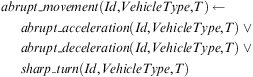 $$\matrix { {abrupt\_movement{\rm{(}}Id{\rm{,}}VehicleType{\rm{,}}T{\rm{)}} \leftarrow } \hfill \cr\ {\; \; \; \; abrupt\_acceleration{\rm{(}}Id{\rm{,}}VehicleType{\rm{,}}T{\rm{)}}\; \vee } \hfill \cr\ {\; \; \; \; abrupt\_deceleration{\rm{(}}Id{\rm{,}}VehicleType{\rm{,}}T{\rm{)}}\; \vee } \hfill \cr\ {\; \; \; \; sharp\_turn{\rm{(}}Id{\rm{,}}VehicleType{\rm{,}}T{\rm{)}}} \hfill \\\end{}$$
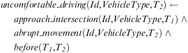 $$ \matrix { {uncomfortable\_driving{\rm{(}}Id{\rm{,}}VehicleType{\rm{,}}{{T}_{\it 2}}{\rm{)}} \leftarrow } \hfill \cr\ {\; \; \; \; approach\_intersection{\rm{(}}Id{\rm{,}}VehicleType{\rm{,}}{{T}_{\it 1}}{\rm{)}}\; \wedge } \hfill \cr\ {\; \; \; \; abrupt\_movement{\rm{(}}Id{\rm{,}}VehicleType{\rm{,}}{{T}_{\it 2}}{\rm{)}}\; \wedge } \hfill \cr\ {\; \; \; \; before{\rm{(}}{{T}_{\it 1}}{\rm{,}}{{T}_{\it 2}}{\rm{)}}} \hfill \\\end{} $$
Variables, starting with upper-case letters, are universally quantified unless otherwise indicated. Predicates and constants start with a lower-case letter. The definition of uncomfortable_driving is simplified here, in order to facilitate the presentation of reasoning techniques in the following section. According to the above formulas, uncomfortable_driving is defined in terms of an auxiliary construct, abrupt_movement, which is in turn defined in terms of the abrupt_acceleration, abrupt_deceleration and sharp_turn LLE. before is a simple predicate comparing two time-points. Formulas (14) and (15) are associated with real-valued positive weights.
MLN facilitate a mixture of soft constraints and hard constraints in a HLE knowledge base, where hard constraints correspond to formulas with infinite weight values. Hard constraints can be used to capture domain-specific knowledge or facts. For example, a bus is driven only by one driver at a time. Soft constraints, on the other hand, can be used to capture imperfect logical statements and their weights provide their confidence value. Strong weights are given to formulas that are almost always true. For instance, we may assign a strong weight to formula (15), as it is true most of the time. Respectively, weak weights may be assigned to formulas that describe exceptions. For example, we may assign a weak weight to the formula stating that ‘unsafe driving’ is recognized when we have ‘abrupt movement’, as normally a ‘very abrupt movement’ is needed for the recognition of ‘unsafe driving’.
4.2 Reasoning
A MLN L is a template that produces a ground Markov network ML,C by grounding all its formulas F, using a finite set of constants  $ C\: = \:{{c}_1}, \ldots \,{{c}_{|C|}} $. More precisely, all formulas are translated into clausal form, where the weight of each formula is equally divided among its clauses, and then the produced clauses are grounded. For different sets of constants, the same MLN L will produce different ground Markov networks, but all will have certain regularities in structure and parameters—for example, all groundings of a clause will have the same weight. Each node in a ML,C is represented by a Boolean variable and corresponds to a possible grounding of a predicate that appears in L. Each subset of ground predicates, appearing in the same ground clause, are connected to each other and form a clique in ML,C. Each clique is associated with the corresponding weight wi of a clause and a Boolean feature. The value of the feature is 1 when the ground clause is true, otherwise it is 0.
A ground Markov network ML,C, therefore, comprises nodes that correspond to a set X of random variables (ground predicates). A state  $ x\: \in \:{\scr X} $ of ML,C represents a possible world, as it assigns truth values to all random variables in X. A probability distribution over states is specified by the ground Markov network ML,C, and represented as follows:
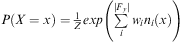 $$\matrix { {P(X\: = \:x)\: = \:\frac{1}{Z}exp\left( {\mathop{\sum}\limits_i^{|{{F}_y}|} {{{w}_i}{{n}_i}(x)} } \right)} \hfill \\\end{}$$
where  $ {{F}_y}\: \subseteq \:F $ is the set of clauses, wi is the weight of the ith clause, ni(x) is the number of true groundings of the ith clause in x and Z is the partition function used for normalization, that is,
 $ Z\: = \:\mathop{\sum}\nolimits_{x\: \in \:{\scr X}} exp(\mathop{\sum}\nolimits_i^{|{{F}_y}|} {{w}_i}{{n}_i}(x)) $, where
 $ \scr X $ is the set of all possible states.
We will illustrate the process of producing a ground Markov network and computing the probability of a state of such a network using the HLE definition expressed by formulas (14) and (15). These formulas are first translated into clausal form:
 $$\frac{1}{3}{{w}_1}\; \; \neg abrupt\_acceleration{\rm{(}}Id{\rm{,}}\ VehicleType{\rm{,}}\ T{\rm{)}} \vee abrupt\_movement{\rm{(}}Id{\rm{,}}\ VehicleType{\rm{,}}\ T{\rm{)}} \ $$
 $$\frac{1}{3}{{w}_1}\; \; \neg abrupt\_deceleration{\rm{(}}Id{\rm{,}}\ VehicleType{\rm{,}}\ T{\rm{)}} \vee abrupt\_movement{\rm{(}}Id{\rm{,}}\ VehicleType{\rm{,}}\ T{\rm{)}} \,\ \,$$
 $$ \matrix { {\displaystyle\frac{1}{3}{{w}_1}\; \; \neg sharp\_turn{\rm{(}}Id{\rm{,}}\ VehicleType{\rm{,}}\ T{\rm{)}} \vee abrupt\_movement{\rm{(}}Id{\rm{,}}\ VehicleType{\rm{,}}\ T{\rm{)}}}\qquad \quad \ \ \, \ \,\hfill \\\end{}$$
 $$\matrix { {{w}_2}\; \; \; \; \neg approach\_intersection{\rm{(}}Id{\rm{,}}\ VehicleType{\rm{,}}\ {{T}_{\it 1}}{\rm{)}} \vee \neg abrupt\_movement{\rm{(}}Id{\rm{,}}\ VehicleType{\rm{,}}\ {{T}_{\it 2}}{\rm{)}} \;\vee \cr\quad\ \; \; \; \; \; \; \;\neg before{\rm{(}}{{T}_{\it 1}}{\rm{,}}{{T}_{\it 2}}{\rm{)}} \vee uncomfortable\_driving{\rm{(}}Id{\rm{,}}\ VehicleType{\rm{,}}\ {{T}_{\it 2}}{\rm{)}} \hfill\\ \end{}$$
where w 1 is the weight of formula (14)—w 1 is equally divided among the three clauses of this formula—while w 2 is the weight of formula (15).
In event recognition, the detected LLEs provide the constants C that are necessary for producing ground Markov networks expressing a knowledge base of HLE definitions—see Figure 7. Consider, for example, a narrative of LLE about tram tr 0 taking place at time-points 100 and 101. The constants involved in this narrative—tr0, tram, 100, 101—define the domain of the corresponding variables—Id, VehicleType, T, T1, T2. If more LLEs were included in the input narrative then the variable domains would have been extended. The grounding procedure produces, in this example, 16 ground predicates and 10 ground clauses. For example, clause (17) is grounded as follows:
Ground Markov Network Construction for Event Recognition. HLE = high-level events; LLE = low-level events

 $$\frac{1}{3}{{w}_{\tf="Times-i" 1}}\; \; \neg abrupt\_acceleration{\rm{(}}t{{r}_{\tf="Times-i" 0}}{\rm{,}}tram{\rm{,}}{\tf="Times-i" 100}{\rm{)}}\; \vee abrupt\_movement{\rm{(}}t{{r}_{\tf="Times-i" 0}}{\rm{,}}tram{\rm{,}}{\tf="Times-i" 100}{\rm{)}}$$
 $$ \frac{1}{3}{{w}_{\tf="Times-i" 1}}\; \; \neg abrupt\_acceleration{\rm{(}}t{{r}_{\tf="Times-i" 0}}{\rm{,}}tram{\rm{,}}{\tf="Times-i" 101}{\rm{)}}\; \vee abrupt\_movement{\rm{(}}t{{r}_{\tf="Times-i" 0}}{\rm{,}}tram{\rm{,}}{\tf="Times-i" 101}{\rm{)}} $$
Similarly, clause (20) is grounded as follows:
 $$ \matrix { {{w}_{\tf="Times-i" 2}}\; \; \neg approach\_intersection{\rm{(}}t{{r}_{\tf="Times-i" 0}}{\rm{,}}tram{\rm{,}}{\tf="Times-i" 100}{\rm{)}}\; \vee \neg abrupt\_movement{\rm{(}}t{{r}_{\tf="Times-i" 0}}{\rm{,}}tram{\rm{,}}{\tf="Times-i" 100}{\rm{)}}\; \vee \cr\quad \; \; \; \; \;\neg before{\rm{(}}{\tf="Times-i" 100}{\rm{,}}{\tf="Times-i" 100}{\rm{)}} \vee uncomfortable\_driving{\rm{(}}t{{r}_{\tf="Times-i" 0}}{\rm{,}}tram{\rm{,}}{\tf="Times-i" 100}{\rm{)}} \hfill\\ \end{} $$
 $$ \matrix { {{{w}_{\tf="Times-i" 2}}\; \; \neg approach\_intersection{\rm{(}}t{{r}_{\tf="Times-i" 0}}{\rm{,}}tram{\rm{,}}{\tf="Times-i" 100}{\rm{)}}\; \vee \neg abrupt\_movement{\rm{(}}t{{r}_{\tf="Times-i" 0}}{\rm{,}}tram{\rm{,}}{\tf="Times-i" 101}{\rm{)}}\; \vee } \hfill \cr\quad {\; \; \; \; \;\neg before{\rm{(}}{\tf="Times-i" 100}{\rm{,}}{\tf="Times-i" 101}{\rm{)}} \vee uncomfortable\_driving{\rm{(}}t{{r}_{\tf="Times-i" 0}}{\rm{,}}tram{\rm{,}}{\tf="Times-i" 101}{\rm{)}}} \hfill \\\end{} $$
 $$ \matrix { {{{w}_{\tf="Times-i" 2}}\; \; \neg approach\_intersection{\rm{(}}t{{r}_{\tf="Times-i" 0}}{\rm{,}}tram{\rm{,}}{\tf="Times-i" 101}{\rm{)}}\; \vee \neg abrupt\_movement{\rm{(}}t{{r}_{\tf="Times-i" 0}}{\rm{,}}tram{\rm{,}}{\tf="Times-i" 100}{\rm{)}}\; \vee } \hfill \cr\quad {\; \; \; \; \;\neg before{\rm{(}}{\tf="Times-i" 101}{\rm{,}}{\tf="Times-i" 100}{\rm{)}} \vee uncomfortable\_driving{\rm{(}}t{{r}_{\tf="Times-i" 0}}{\rm{,}}tram{\rm{,}}{\tf="Times-i" 100}{\rm{)}}} \hfill \\\end{} $$
 $$ \matrix { {{{w}_{\tf="Times-i" 2}}\; \; \neg approach\_intersection{\rm{(}}t{{r}_{\tf="Times-i" 0}}{\rm{,}}tram{\rm{,}}{\tf="Times-i" 101}{\rm{)}}\; \vee \neg abrupt\_movement{\rm{(}}t{{r}_{\tf="Times-i" 0}}{\rm{,}}tram{\rm{,}}{\tf="Times-i" 101}{\rm{)}}\; \vee } \hfill \cr\quad {\; \; \; \; \;\neg before{\rm{(}}{\tf="Times-i" 101}{\rm{,}}{\tf="Times-i" 101}{\rm{)}} \vee uncomfortable\_driving{\rm{(}}t{{r}_{\tf="Times-i" 0}}{\rm{,}}tram{\rm{,}}{\tf="Times-i" 101}{\rm{)}}} \hfill \\\end{} $$
The resulting ground Markov network is shown in Figure 8. Predicates appearing in the same ground clause are connected to each other in the network and form a clique. Consider, for instance, the clique created by ground clause (17a) consisting of abrupt_acceleration(tr0, tram, 100) and abrupt_movement(tr0, tram, 100). The clique is associated with the weight of the corresponding clause, that is,  $ \tfrac{1}{3}{{w}_1} $, and a Boolean feature. In a state where abrupt_movement(tr0, tram, 100) is true, the grounding (17a) of clause (17) is satisfied and therefore the value of the feature is 1.
Ground Markov Network

We will illustrate how the probability of each state of a ground Markov network is computed by calculating the probability of two possible states, x 1 and x 2, of the network shown in Figure 8. Assume that both x 1 and x 2 assign the same truth values to all predicates except uncomfortable_driving(tr0, tram, 101). More precisely, in both states approach_intersection(tr0, tram, 100), abrupt_acceleration(tr0, tram, 101), abrupt_movement(tr0, tram, 101) and before(100, 101) are true. All the other ground predicates are false, except uncomfortable_driving(tr0, tram, 101) being true in x 1 and false in x 2. In this example, the weights w 1 and w 1 of formulas (14) and (15) are positive real numbers. The number of satisfied groundings of clauses (17), (18) and (19) is the same in both x 1 and x 2, as the assignment of truth values to the predicates involved is the same. The number of satisfied groundings of clause (20), however, differs between x 1 and x 2, because the truth assignment of uncomfortable_driving(tr0, tram, 101) is different. As a result, in state x 1 all ground clauses of (20) are satisfied, but in state x 2 ground clause (20b) is not satisfied. Using Equation (16) we compute the following:
 $$\displaylines{ & P(X\: = \:{{x}_1})\: = \:\frac{1}{Z}\,exp\left( {\frac{1}{3}{{w}_1}\:\times \:2\: + \:\frac{1}{3}{{w}_1}\:\times \:2\: + \:\frac{1}{3}{{w}_1}\:\times \:2\: + \:{{w}_2}\:\times \:4} \right)\: = \:\frac{1}{Z}{{e}^{2{{w}_1}\: + \:4{{w}_2}}} \cr & P(X\: = \:{{x}_2})\: = \:\frac{1}{Z}\,exp\left( {\frac{1}{3}{{w}_1}\:\times \:2\: + \:\frac{1}{3}{{w}_1}\:\times \:2\: + \:\frac{1}{3}{{w}_1}\:\times \:2\: + \:{{w}_2}\:\times \:3} \right)\: = \:\frac{1}{Z}{{e}^{2{{w}_1}\: + \:3{{w}_2}}} \cr}$$
According to the above results, a state (x 1) in which the ‘uncomfortable driving’ HLE and its sub-events have all been recognized is more probable than a state (x 2) in which the sub-events of ‘uncomfortable driving’ have been recognized while this HLE does not hold.
Event recognition in MLN involves querying a ground Markov network about HLE. The set X of random variables of a ground network can be partitioned as  $ X\: = \:Q\: \cup \:E\: \cup \:H $, where Q is the set of ‘query variables’, E is the set of ‘evidence variables’ and H is the set of the remaining variables with unknown value—also known as ‘hidden variables’. In event recognition, query variables represent the HLE of interest, evidence variables represent the detected LLE, while hidden variables represent auxiliary constructs of a HLE definition. Event recognition queries require conditional inference, that is, computing the probability that a query variable holds given some evidence. For the computation of conditional probabilities a variety of exact and approximate probabilistic inference methods exist in the literature. Given a MLN and some evidence E = e, a conditional query is specified as follows:
 $$P(Q\:|\:E\: = \:e,H)\: = \:\frac{{P(Q,E\: = \:e,H)}}{{P(E\: = \:e,H)}}$$
where Q's are the query variables and H's are the hidden variables. The numerator and denominator of this equation may be computed using Equation (16). We may be interested in finding out, for instance, the trams that are driven in an uncomfortable manner, given a LLE narrative. In this case, the set of query variables Q includes only uncomfortable_driving(Id, VehicleType, T), the set of detected LLE that forms E may include, among others
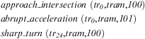 $$ \matrix { approach\_intersection\ {\rm{(}}t{{r}_{\tf="Times-i" 0}}{\rm{,}}tram{\rm{,}}{\tf="Times-i" 100}{\rm{)}} \cr\ abrupt\_acceleration\ {\rm{(}}t{{r}_{\tf="Times-i" 0}}{\rm{,}}tram{\rm{,}}{\tf="Times-i" 101}{\rm{)}} \quad \ \hfill\cr\ sharp\_turn\ {\rm{(}}t{{r}_{{\tf="Times-i" 24}}}{\rm{,}}tram{\rm{,}}{\tf="Times-i" 100}{\rm{)}} \qquad \ \ \qquad \\ \end{} $$
and the set of hidden variables H includes, among others
 $$ \matrix { abrupt\_movement\ {\rm{(}}t{{r}_{\tf="Times-i" 0}}{\rm{,}}tram{\rm{,}}{\tf="Times-i" 101}{\rm{)}} \quad \ \ \cr\ abrupt\_movement\ {\rm{(}}t{{r}_{\tf="Times-i" 24}}{\rm{,}}tram{\rm{,}}{\tf="Times-i" 101}{\rm{)}} \quad \ \ \end{} $$
Given Equation (21), we may compute the probability of each grounding of uncomfortable_driving(Id, VehicleType, T).
Complete grounding of MLN, even for simple HLE knowledge bases, results in complex and large networks. For this reason, only the minimal required network is constructed to answer a conditional query. In particular, query and evidence variables are used to separate the network into regions, allowing some variables to be removed from the network, as they cannot influence reasoning. For example, given the Markov network shown in Figure 8, we may be interested only in the HLE uncomfortable_driving(tr0, tram, 101). The truth values of ground before predicates are trivially known. Moreover, the truth values of LLE are given as evidence—see Figure 9(a). The nodes for the ground predicates abrupt_movement(tr 0, tram, 100), uncomfortable_driving(tr0, tram, 100), sharp_turn(tr0, tram, 100), abrupt_deceleration(tr0, tram, 100), before(100, 100) and before(101, 100) can be omitted from the Markov network, as they cannot influence the reasoning process concerning the HLE uncomfortable_driving(tr0, tram, 101). Therefore, the complete Markov network, shown in Figure 9(a), will be reduced into the network shown in Figure 9(b).
(a) Complete Ground Markov Network and (b) Ground Markov Network Reduced for Event Recognition. Nodes with a thick line represent query variables, shaded nodes represent variables with known truth values and nodes with a dashed line represent variables that can be safely removed

Further efficiency can be gained by using (a) lazy inference methods that ground predicates as and when needed (Singla & Domingos, Reference Singla and Domingos2006; Domingos & Lowd, Reference Domingos and Lowd2009; Section 3.3) or (b) lifted inference methods which can answer queries without grounding the entire network (Singla & Domingos, Reference Singla and Domingos2008; Domingos & Lowd, Reference Domingos and Lowd2009).
Sensors may detect LLE with certainty or with a degree of confidence. In the former case, the LLEs are simple Boolean variables that are given directly to the MLN as evidence. In the latter case, the detected LLEs are usually added to the MLN knowledge base as clauses having weights proportional to their detection probability (Tran & Davis, Reference Tran and Davis2008). For example, if the LLE sharp_turn(tr0, tram, 20) is detected with some probability P(sharp_turn(tr0, tram, 20)), the unit clause sharp_turn(tr0, tram, 20) will be added to the MLN with weight value
 $$ \matrix { {w\: = \:\log \displaystyle {\frac{{P{\rm{(}}sharp\_turn(t{{r}_{\tf="Times-i" 0}}{\rm{,}}tram{\rm{,}}{\tf="Times-i" 20}{\rm{))}}}}{{{\tf="Times-i" 1}{\rm{ - }}P(sharp\_turn(t{{r}_{\tf="Times-i" 0}}{\rm{,}}tram{\rm{,}}{\tf="Times-i" 20}{\rm{))}}}}} \hfill \\\end{} $$
The additional clauses, which represent the detected LLE with a degree of confidence, alter the posterior distribution over possible worlds by introducing additional features in the ground Markov network. In this manner, the detected LLEs propagate their degree of confidence to the whole MLN.
Even in a very large state space, the computation of Equation (21) can be efficiently approximated by sampling methods, such as Markov Chain Monte Carlo (MCMC) algorithms—for example, Gibbs sampling. Markov Chains form graphs of possible states, over which a Monte Carlo simulation takes a random walk and draws a set of sample states from the target distribution. In MCMC, a successive sample state depends only on the current state. In Gibbs sampling, for instance, each sample state is produced by successively changing the truth value assignment of its ground predicates. This reassignment of truth values is performed efficiently, as the value of each predicate in the ground Markov network depends only on the truth values of its neighbour predicates. The set of neighbouring predicates is called Markov blanket and represents predicates that appear together in some grounding of a clause. For instance, the Markov blanket of abrupt_movement(tr0, tram, 101) in the network shown in Figure 8 is composed of uncomfortable_driving(tr0, tram, 101), before(100, 101), approach_intersection(tr0, tram, 100), sharp_turn(tr0, tram, 101), abrupt_acceleration(tr0, tram, 101), abrupt_deceleration(tr0, tram, 101), approach_intersection(tr0, tram, 101) and before(100, 101). The conditional probability in Equation (21) can be computed by a MCMC algorithm that rejects all moves to states where E = e does not hold. Therefore, only the variables that belong to Q and H are allowed to change in each sample. In each step, the MCMC algorithm has the tendency to keep samples that represent states with high probability and, therefore, often converges in local maxima. The estimated probability of the query variables, that is, the HLE of interest, is the fraction of samples in which those variables are true. The more samples are generated, the more accurate this estimation becomes.
Due to the combination of logic with probabilistic models, inference in MLN must handle both deterministic and probabilistic dependencies. Deterministic or near-deterministic dependencies are formed from formulas with infinite and strong weights, respectively. Being a purely statistical method, MCMC can only handle probabilistic dependencies. In the presence of deterministic dependencies, two important properties of Markov Chains, ergodicity and detailed balance, are violated and the sampling algorithms give poor results (Poon & Domingos, Reference Poon and Domingos2006). Ergodicity is satisfied if all states are aperiodically reachable from each other, while detailed balance is satisfied if the probability of moving from state xi to state xj is the same as the probability of moving from xj to xi. Ergodicity and detailed balance are violated in the presence of deterministic dependencies because these dependencies create isolated regions in the state space by introducing zero-probability (impossible) states. Even near-deterministic dependencies create regions that are difficult to cross, that is, contain states with near zero-probability. As a result, typical MCMC methods, such as Gibbs sampling, get trapped in local regions. Thus, they are unsound for deterministic dependencies and they find it difficult to converge in the presence of near-deterministic ones.
To overcome these issues and deal with both deterministic and probabilistic dependencies, MLN use the MC-SAT algorithm (Poon & Domingos, Reference Poon and Domingos2006; Domingos & Lowd, Reference Domingos and Lowd2009; Section 3.2), which is a MCMC method that combines satisfiability testing with slice-sampling (Damlen et al., Reference Damlen, Wakefield and Walker1999). Initially, a satisfiability solver is used to find those assignments that satisfy all hard-constrained clauses (i.e clauses with infinite weights). At each subsequent sampling step, MC-SAT chooses from the set of ground clauses satisfied by the current state the clauses that must be satisfied at the next step. Each clause is chosen with probability proportional to its weight value. Clauses with infinite or strong weights, that represent, respectively, deterministic and near-deterministic dependencies, will always be chosen with, respectively, absolute certainty and high probability. Then, instead of taking a sample from the space of all possible states, slice-sampling restricts sampling to the states that satisfy at least all chosen clauses. In this manner, MCMC cannot get trapped to local regions, as satisfiability testing helps to collect samples from all isolated and difficult-to-cross regions.
4.3 Machine learning
Learning a MLN involves estimating the weights of the network and/or the first-order rules forming the network structure, given a set of training data, that is, LLE annotated with HLE. In Section 4.3.1, we present approaches on weight learning while in Section 4.3.2 we discuss structure learning.
4.3.1 Weight learning
Weight learning concerns the estimation of the weights of the clauses that represent a HLE knowledge base—recall that the first-order rules of such a knowledge base are translated into clausal form. Different clauses, derived from the same rule, may be assigned different weights. For example, it may be estimated that the weights of the clauses derived from rule (14) are different:
 $$ {{w}_a}\; \; \neg abrupt\_acceleration{\rm{(}}Id{\rm{,}}\,VehicleType{\rm{,}}\,T{\rm{)}} \vee abrupt\_movement{\rm{(}}Id{\rm{,}}\,VehicleType{\rm{,}}\,T{\rm{)}} $$
 $${{w}_b}\; \; \neg abrupt\_deceleration{\rm{(}}Id{\rm{,}}\,VehicleType{\rm{,}}\,T{\rm{)}} \vee abrupt\_movement{\rm{(}}Id{\rm{,}}\,VehicleType{\rm{,}}\,T{\rm{)}}$$
 $$ \matrix { {{{w}_c}\; \; \neg sharp\_turn{\rm{(}}Id{\rm{,}}\,VehicleType{\rm{,}}\,T{\rm{)}} \vee abrupt\_movement{\rm{(}}Id{\rm{,}}\,VehicleType{\rm{,}}\,T{\rm{)}}} \qquad \qquad \hfill \\\end{} $$
Weight learning in MLN is performed by optimizing a likelihood function, which is a statistical measure of how well the probabilistic model (MLN) fits the training data. In particular, weights can be learned by either generative or discriminative estimation (Singla & Domingos, Reference Singla and Domingos2005; Lowd & Domingos, Reference Lowd and Domingos2007; Huynh & Mooney, Reference Huynh and Mooney2008; Domingos & Lowd, Reference Domingos and Lowd2009; Section 4.1). Generative learning attempts to optimize the joint distribution of all variables in the model. In contrast, discriminative learning attempts to optimize the conditional distribution of a set of outputs, given a set of inputs.
Generative estimation methods search for weights that optimize the likelihood function, given a HLE knowledge base and training data. Learning can be performed by a standard gradient ascent optimization algorithm. However, it has been shown that computing the likelihood and its gradient is intractable (Richardson & Domingos, Reference Richardson and Domingos2006). For this reason, the optimization of the pseudo-likelihood function is used instead, which is the product of the probabilities of the ground predicates, conditioned on their neighbours in the network, that is, their Markov blanket. In particular, if x is a state of a ground network and xl is the truth value of the lth ground predicate Xl, the pseudo-likelihood of x, given weights w, is:
 $$\matrix { {\log \:P_{w}^{\ast} {\rm{(}}X\: = \:x{\rm{)}}\: = \:\mathop{\sum}\limits_{l\: = \:1}^n {\log \:{{P}_w}{\rm{(}}{{X}_l}\: = \:{{x}_l}\:|\:M{{B}_x}{\rm{(}}{{X}_l}{\rm{))}}} } \hfill \\\end{}$$
 $ M{{B}_x}{\rm{(}}{{X}_l}{\rm{)}} $ represents the truth values of the ground predicates in the Markov blanket of Xl. Thus, computation can be performed very efficiently, even in domains with millions of ground predicates, as it does not require inference over the complete network.
The pseudo-likelihood function assumes that each ground predicate's Markov blanket is fully observed, and does not exploit information obtained from longer-range dependencies in the network. In some cases this assumption may lead to poor results. Consider, for example, formulas (14) and (15) expressing, respectively, abrupt_movement and uncomfortable_driving, and a training data set including a LLE narrative annotated only for uncomfortable_driving, that is, there is no annotation for abrupt_movement. Figure 10 displays the resulting ground Markov network. As mentioned in Section 4.2, the Markov blanket of abrupt_movement includes the sharp_turn, abrupt_acceleration and abrupt_deceleration LLE. The Markov blanket of uncomfortable_driving includes abrupt_movement. In this case, pseudo-likelihood may give poor results with respect to the uncomfortable_driving HLE. This is due to the fact that it will only use information from the Markov blanket of this HLE, making an assumption about the absent annotation of abrupt_movement—usually a closed-world assumption. In other words, it will not exploit the information provided by the abrupt_acceleration, abrupt_deceleration and sharp_turn LLE of the training data set.
Ground Markov Network Produced from Partially Annotated Data set. The shaded nodes represent predicates with known truth values as described in the annotated data set

One way to address the aforementioned issue is to treat absent annotations as missing information and use the expectation maximization algorithm of Dempster et al. (Reference Dempster, Laird and Rubin1977) in order to learn from incomplete data (Poon & Domingos, Reference Poon and Domingos2008; Domingos & Lowd, Reference Domingos and Lowd2009; Section 4.3).
In event recognition, we know a priori which variables form the evidence (LLE) and which ones concern queries (HLE). In the usual case, where we aim to recognize the latter given the former, it is preferable to learn the weights discriminatively by maximizing the conditional likelihood function. In particular, if we partition the variables of the domain into a set of evidence variables E and a set of query variables Q, then the conditional likelihood function is defined as follows:
 $$\matrix { {\log \:P(Q\: = \:q\:|\:E\: = \:e)\: = \:\mathop{\sum}\limits_i {{w}_i}{{n}_i}(e,y){\rm{ - }}\log \:{{Z}_e}} \hfill \\\end{}$$
where Ze normalizes over all states consistent with the evidence e, and ni(e, y) is the number of true groundings of the ith clause in the training data set. In contrast to Q and E, the state of a hidden variable, such as abrupt_movement, is unknown as, in most cases, the state of such variables is not available in the training dataset. In the presence of hidden variables, therefore, the conditional likelihood must be computed by marginalizing over the hidden variables. It has been shown that learning weights discriminatively can lead to higher predictive accuracy than generative learning (Singla & Domingos, Reference Singla and Domingos2005). This is partly due to the fact that, in contrast to the pseudo-likelihood function, conditional likelihood can exploit information from longer-range dependencies. Similar to the likelihood function, conditional likelihood requires inference. However, there is one key difference: conditioning on the evidence in a Markov network reduces significantly the number of likely states. Therefore, inference takes place on a simpler model and the computational requirements are reduced.
Weights in MLN are estimated using either first-order or second-order optimization methods. First-order methods, for example, perform gradient ascent optimization in order to maximize an evaluation function, such as the conditional likelihood function (26). Weights may be initialized to zero, they may be given random values, or they may be given values according to other information concerning the application under consideration. Then, weights are iteratively updated according to the following equation:
 $${{{\rm{\tf="AgfaRSSB" w}}}_{t\: + \:1}}\: = \:{{{\rm{\tf="AgfaRSSB" w}}}_t}\: + \:\eta {\rm{\tf="AgfaRSSB" g}}$$
where t indicates the current iteration of the optimization process, w t is a vector that contains weight values of the current iteration for all clauses in the knowlege base, while w t +1 is a vector that contains the updated weight values. The constant η expresses the learning rate, defining the extent of weight adjustment in each iteration. The vector w represents the gradient. This is composed of the partial derivatives of function (26) with respect to the corresponding clause weights. The value of a derivative defines the direction and the magnitude of a weight update. The computation of the gradient requires inference, which can be efficiently approximated using MCMC methods, as discussed in Section 4.2.
By iteratively adjusting the weights using Equation (27), the fit of the model to the HLE in the data set is optimized. Assume, for example, that in a given training data set the abrupt_acceleration LLE is rarely associated with the occurrence of the HLE uncomfortable_driving. On the other hand, the abrupt_deceleration and sharp_turn LLEs are closely associated with the HLE uncomfortable_driving. In this case, weight learning will assign a low weight value to clause (22) and high weight values to clauses (23) and (24).
4.3.2 Structure learning
In addition to weight learning, the structure of a MLN can be learned from training data. In principle, the structure of a MLN can be learned in two stages, using any ILP method, as presented in Section 2.3, and then performing weight learning. However, separating the two learning tasks in this way may lead to suboptimal results, as the first optimization step (ILP) needs to make assumptions about the weight values, which have not been optimized yet. Better results can be obtained by combining structure learning with weight learning in a single stage.
A variety of structure learning methods have been proposed for MLN. In brief, these methods can be classified into top-down and bottom-up methods. Top-down structure learning (Kok & Domingos Reference Kok and Domingos2005; Domingos & Lowd Reference Domingos and Lowd2009; Section 4.2) starts from an empty or existing MLN and iteratively constructs clauses by adding or revising a single predicate at a time, using typical ILP operations and a search procedure. However, as the structure of a MLN may involve complex HLE definitions, the space of potential top-down refinements may become intractable. For this reason, bottom-up structure learning can be used instead, starting from training data and searching for more general hypotheses (Mihalkova & Mooney, Reference Mihalkova and Mooney2007; Domingos & Lowd, Reference Domingos and Lowd2009; Kok & Domingos, Reference Kok and Domingos2009, Reference Kok and Domingos2010; Section 4.2). This approach usually leads to a more specialized model, following a search through a manageable set of generalizations.
5 Summary and open issues
We presented three representative logic-based approaches to event recognition. All approaches assume as input a stream of time-stamped LLE—a LLE is created as a result of applying a computational derivation process to some other event. Using such input, event recognition systems identify HLE of interest, that is, collections of events that satisfy some pattern. We illustrated the use of the three reviewed approaches drawing examples from the domain of CTM.
Being based on logic, all three approaches benefit from a formal and declarative semantics, a variety of inference mechanisms, and methods for learning a knowledge base of HLE definitions from data. As a result, compared with procedural methods, logic-based ones facilitate efficient development and management of HLE definitions, which are clearly separated from the generic inference mechanism. Moreover, compared with methods exhibiting informal semantics, logic-based approaches support validation and traceability of results. At the same time, recent logic-based methods appear to be sufficiently mature and scalable to be used in industrial applications.
The presented CRS has been specially developed for event recognition and is the choice of preference for efficient, purely temporal recognition. CRS was developed with the aim to support only temporal reasoning and thus a line of future work concerns its extension with atemporal reasoning. The developers of CRS are currently making it open-source (C. Dousson, personal communication), thus facilitating extensions of its reasoning engine.
The EC provides a more generic and expressive representation of HLE definitions, taking advantage of the full power of logic programming on which it is based. Thus, EC supports complex temporal as well as atemporal representation and reasoning. A line of further work concerns the optimization of the reasoning of EC for run-time event recognition. Caching techniques, in particular, should be investigated, supporting all types of HLE representation.
MLN combine the strengths of logical and probabilistic inference. Consequently, they may address, to a certain extent, the issues of incomplete LLE streams, erroneous LLE detection, inconsistent LLE and HLE annotation and limited dictionary of LLE and context variables. This is in contrast to CRS and EC that do not consider uncertainty in representation and reasoning. MLNs also offer a very expressive framework for HLE definition representation, as the full power of first-order logic is available. The use of MLN for event recognition, however, has been limited so far and there are many issues that need to be resolved still, such as the incorporation and use of numerical temporal constraints in MLN inference.
Finally, a number of challenging issues remain open in learning HLE definitions. Examples of such issues are the use of abduction to handle partial supervision in large data sets that is commonly available for event recognition, and the simultaneous optimization of numerical parameters—for example, weights and temporal constraints—and the logical structure of the knowledge base expressing HLE definitions.
Acknowledgements
This work has been partially funded by EU, in context of the PRONTO project (FP7-ICT 231738). Francois Portet is supported by the French national project Sweet-Home (ANR-09-VERS-011).
This paper is a significantly updated and extended version of Artikis et al. (Reference Artikis, Paliouras, Portet and Skarlatidis2010a). The authors would like to thank the reviewers and participants of the Fourth International Conference on Distributed Event-Based Systems, as well as the reviewers of the Knowledge Engineering Review, who gave us useful feedback.
They would also like to thank Christophe Dousson for his suggestions regarding the Chronicle Recognition System. The authors themselves, however, are solely responsible for any misunderstanding about the use of this technology.