1. Introduction

Like many scientific concepts, fully adequate definitions of some ecological concepts have not yet been formulated. Ecological stability is one such concept. Proposed definitions of it are not fully satisfactory and, worse, seem incompatible (Shrader-Frechette and McCoy Reference Shrader-Frechette and McCoy1993). Although it is incorrect to conclude from this that the concept itself is problematic (Odenbaugh Reference Odenbaugh2001), the multitude of incompatible definitions initiates and exacerbates conceptual confusion.

Among mathematical ecologists, ecological stability is commonly defined as Lyapunov stability, named after the Russian mathematician who first precisely defined the concept to describe the apparently stable equilibrium behavior of the solar system (Lyapunov Reference Lyapunov[1892] 1992). His definition has found widespread application outside this context and is frequently used to analyze mathematical models of biological communities (Logofet Reference Logofet1993). May (Reference May1974) used this definition, for instance, in his influential analysis of relationships between the stability and complexity of such models.

The definition has some clear advantages. Unlike other definitions, it integrates ecological stability into a thoroughly studied mathematical theory that has proved fruitful in many sciences, especially mathematical physics. It also seems to formalize the intuition that ecological stability depends on community response to perturbation. Despite these apparent advantages, ecological stability should not be defined as Lyapunov stability.

Sections 2 and 3 describe the concept of Lyapunov stability, its underlying mathematical theory, and show why this theory is so successful within physics. Section 4 considers the apparent advantages of the definition and illustrates how Lyapunov stability applies to mathematical models of biological communities. Section 5 argues this definition is problematic, focusing specifically on biological interpretation of Lyapunov stability. Based on this analysis, Section 6 draws some general conclusions about scientific definition and highlights an important difference between dynamic systems modeling in physics and in ecology.

2. Lyapunov Stability

To ensure sufficient generality, represent a system by a position vector x(t) (t represents time) in a n-dimensional Euclidean state space E. Assume E is governed by a vector function F representing the magnitude and change of direction it induces on x(t). F represents, therefore, the factors responsible for the dynamics of the system x(t) represents. Points in E for which $\mathbf{F}=0$ are called equilibrium points, and unperturbed position vectors at such points remain stationary.

Lyapunov stability (‘L-stability’ hereafter) is a property of system behavior in neighborhoods of equilibria. Specifically, an equilibrium x* is Lyapunov stable (‘L-stable’ hereafter) in $E_{x}( \mathbf{x}^{\mathbf{*}}\in E_{x}\subseteq E) $ iff

(1)

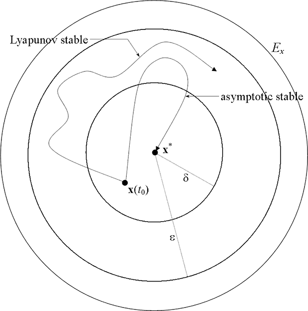
where $\varepsilon \geq \delta $ , $\mathbf{x}( t_{0}) \in E_{x}$ represents the system at some initial time t ₀, and ‘|·|’ designates a Euclidean distance metric on E. The initial displacement from x* to x(t ₀) represents the perturbation to the system. Informally, (1) therefore says x* is L-stable if for any ε-neighborhood of x* a smaller δ-neighborhood can be found such that if the system is perturbed within the δ-neighborhood, it never leaves the ε-neighborhood. x* is asymptotically L-stable if (1) and $\mathrm{\lim}_{t\rightarrow \infty }\mathbf{x}( t) =\mathbf{x}^{*}$ .

If x* is (asymptotically) L-stable on all of E, x* is (asymptotically and) globally L-stable. The subspace E _x of E within which systems can be displaced from an L-stable x* and satisfy (1) nontrivially, that is, the antecedent and consequent of the conditional hold for the relevant quantification, is called the stability domain of x*. The stability domain within which systems can be displaced from an asymptotically L-stable x* and $\mathrm{\lim}_{t\rightarrow \infty }\mathbf{x}( t) =\mathbf{x}^{\mathrm{*}\,}$ is called the attraction domain of x* (see Figure 1).

Figure 1.

Graphical representation of asymptotic and nonasymptotic Lyapunov stability.

In general, L-stability cannot be assessed with (1) because explicit solutions for x(t) can seldom be found. For instance, scientific models often characterize x(t) in terms of differential equations:

(2)

where Ω is a set of parameters designating factors that influence system dynamics but are uninfluenced by them, and F takes the form of an $n\times n$ matrix.Footnote ¹ For complicated systems modeled by (2) that scientists study, however, explicit solutions for x(t) are rarely available. Without such solutions, system behavior as required by (1) cannot be directly evaluated.

3. The Direct and Indirect Methods

Lyapunov (Reference Lyapunov[1892] 1992) recognized this difficulty and developed two methods for assessing (1) indirectly. The first ‘indirect method’ involves linearizing F at x*. Specifically, let

be the Jacobian matrix of F evaluated at x*. The eigenvalues of A determine whether x* is stable. These are scalar values $\lambda _{i}$ such that $\mathrm{det}\,( \mathbf{A}-\lambda _{i}\mathbf{I}) =0$ , that is, the roots of the characteristic polynomial of A. Lyapunov proved x* is asymptotically L-stable if

(3)

where $\mathrm{Re}\,\lambda _{i}( \mathbf{A}) $ designates the real part of the ith eigenvalue of A. Since A is only defined at x*, stability determined by the indirect method is restricted to infinitesimal neighborhoods of x*. For this reason, it is called local stability. The indirect method is prevalent in mathematical modeling because it is almost universally applicable: it applies to any system representable by continuous and continuously differentiable equations, such as (2) (Hinrichsen and Pritchard Reference Hinrichsen and Pritchard2005).

Stability criteria based on the indirect method such as (3) have a serious limitation: they provide no information about the extent of attraction domains. This prompted Lyapunov (Reference Lyapunov[1892] 1992) to develop a ‘direct method’ for evaluating L-stability. It involves constructing a differentiable scalar Lyapunov function (‘L-function’ hereafter) V(x) with an origin at x* (i.e., $\mathbf{x}^{*}=\mathbf{0}$ ) such that:

1. (i) V(x) is positive definite: (a) $V( \mathbf{0}) =0$ ; (b) $V( \mathbf{x}) > 0$ for all $\mathbf{x}\neq \mathbf{0}$ ; and

2. (ii) $\nabla V( \mathbf{x}) \cdot \mathbf{F}( \mathbf{x},\,\Omega ) \leq 0$ for all x,

where ‘·’ and ‘∇’ designate the dot product and gradient vector function. Lyapunov proved the existence of an L-function on $E_{x}\subseteq E$ is sufficient for L-stability of x* in this region, and that with strict inequality in (ii), x* is asymptotically L-stable. This condition was also later proved necessary (Hahn Reference Hahn1963). The ability to construct an L-function is thus a stability criterion. The extent of the attraction domain of an equilibrium can also be evaluated using L-functions (Hahn Reference Hahn1963). As a methodology, it is called ‘direct’ because whether such a function can be constructed depends directly upon the mathematical form of equations like (2), unlike the indirect method, which relies on their linearization to evaluate stability, and unlike direct evaluation of (1), which requires explicit solutions to (2).

Although no general method for constructing L-functions is known, the direct method has proven to be extremely useful in analyzing physical systems, especially in the classical framework governed by only Newtonian mechanics and friction. Across scientific fields, this is exceptional rather than typical. Constructing L-functions is usually extremely difficult for the predominantly nonlinear systems scientists study (Goh Reference Goh1977). The reason for its utility in the classical framework is twofold. First, there are highly confirmed mathematical models describing numerous types of systems in this framework. The likelihood therefore seems high that application of the direct method to these models will reveal the true stability properties of the systems they accurately represent. Second, there are certain quantities, such as total energy, that are conserved or monotonically dissipated in such systems, depending on how they are characterized (e.g., closed or open). These quantities ensure L-functions exist for models of these systems. Lyapunov, in fact, developed the L-function to generalize the classical energy concept, and energy conservation played an important role in his development of the proof about the connection between stability and L-functions (Lyapunov Reference Lyapunov[1892] 1992).

To illustrate, consider a closed particle mass system governed by a conservative force field G in a frictionless Newtonian framework. System energy, V(x, v), is designated by the Hamiltonian

(4)

where x and v are position and velocity vectors, m represents particle mass, ‘|·|’ designates the magnitude of ·, and U is a scalar potential energy function such that $\mathbf{G}( \mathbf{x}) =-\nabla U( \mathbf{x}) $ . Energy conservation ensures

(5)

where c is a constant. At an equilibrium x*, $\mathbf{v}=\mathbf{0}$ , $\mathbf{G}=\mathbf{0}$ , and hence $\nabla U( \mathbf{x}) =\mathbf{0}$ . If x* is also a local minimum of U(x), an ‘energy difference’ function $V^{*}( \mathbf{x},\,\mathbf{v}) $ can be defined: $V^{*}( \mathbf{x},\,\mathbf{v}) =V( \mathbf{x},\,\mathbf{v}) -V( \mathbf{x}^{*},\,\mathbf{0}) $ . $V^{*}( \mathbf{x},\,\mathbf{v}) $ is an L-function and x* is therefore stable. In this case, energy conservation entails the second requirement of L-functions ([ii] from above) is satisfied by equality. If, however, system energy were continually decreasing instead of conserved, depleted by friction for instance, (ii) would be satisfied by strict inequality and x* would be asymptotically stable.

Within the classical framework, stability properties of more complicated models that include and disregard friction can be evaluated with the direct method. The method is also useful in nonclassical frameworks with similar properties, such as mass–energy conservation in special relativity theory. The equations characterizing systems in these and the classical framework are often too complex to solve analytically, and the direct method provides the only means by which attraction domains of equilibria can be determined. In a wide variety of frameworks within physics, therefore, the direct method and concept of L-stability are indispensable.

4. Lyapunov Theory and Community Modeling

The outline of Lyapunov theory above suggests some advantages of defining ecological stability as L-stability. First, the definition formalizes the concept and integrates it into a well-known mathematical theory. Stability properties of community models can then be assessed with analytical techniques like the indirect and direct methods.

Besides the obvious virtues of formalization, L-stability also seems to capture precisely the intuition that ecological stability depends upon community response to perturbation. Consulting (1) and Figure 1, think of a community perturbed at time t ₀ from an L-stable x* to x(t ₀) within the stability domain of x*. Equation (1) then entails that the perturbed community will remain in relevant ε-neighborhoods of x* for $\forall t\geq t_{0}$ , that is, the effects of the perturbation are circumscribed.Footnote ² Some other popular definitions define ecological stability in terms of the variability of populations in a community and are mathematically precise in that they are statistical functions of model variables (e.g., Lehman and Tilman's [Reference Lehman and Tilman2000] “temporal stability”). They do not, however, as L-stability does, provide a mathematical characterization of equilibrium system dynamics. If x* is L-stable, for instance, the conditional in (1) ensures predictions can be made about system behavior after perturbations from x* within its stability domain. Mathematical definitions in the statistical sense cannot ground such predictions unless future values of variables depend upon past values in some systematic way, and the precise form of the dependency is known. The concept of L-stability is an important analytic tool within physics because (1) provides a mathematically precise description of the equilibrium dynamics of systems.

In addition, properties of community response to perturbation that are fundamental components of ecological stability seem to be formalizable with the direct method. The size of attraction domains of asymptotically L-stable equilibria and the rate systems return to them, for instance, are definable in terms of L-functions (Hahn Reference Hahn1963, Sections 12, 22–25). The larger the attraction domain, for instance, the stronger the perturbations of variables a system can sustain and return to x*, which is often called system ‘tolerance’. Similarly, the ‘steeper’ the L-function V(x) (as gauged by ∇V(x)), the faster it returns to x*, often called system ‘resilience’. If L-stability adequately defined ecological stability, it would therefore be possible to formalize the properties of tolerance and resilience and their relation to the stability of biological communities. Specifically, the intuitive idea that ecological stability increases with the strength of perturbation from which a system can return to equilibrium and with the speed of return to equilibrium after perturbation would be formalizable.

Finally, the direct method adequately characterizes the equilibrium dynamics of many systems in physics (and other sciences), and it is reasonable to expect the method will function similarly for ecological systems since their models share a similar mathematical structure. Like systems studied in physics, biological communities are usually modeled by differential equations. The only difference is that components of the vector $\mathbf{x}( t) =\langle x_{1}( t) ,\,\ldots ,\, x_{i}( t) ,\,\ldots ,\, x_{n}( t) \rangle $ represent biological variables, usually population sizes of species in a community, instead of typical physical variables.

This expectation seems to be supported, for instance, by the classical Lotka-Volterra model of one-predator, one-prey communities:

(6a)

(6b)

where x _d and x _y represent predator and prey population sizes, a represents prey birth rate, b represents predator death rate; and $\alpha ,\,\beta > 0$ represent the effect of predator individuals on prey individuals and vice versa. Setting the left sides to 0 and solving yields one nontrivial equilibrium x* where $x^{*}_{d}=b/ \beta $ and $x^{*}_{y}=a/ \alpha $ . An L-function for this equilibrium exists for all $x_{d},\, x_{y}> 0$ :

(7)

where $c_{1},\, c_{2}> 0$ are constants, so x* is globally stable by the direct method (Logofet Reference Logofet1993).

A property of (6) discovered by Vito Volterra reveals an interesting structural similarity between models of ecological and physical systems, which in turn seems to justify the utility of Lyapunov theory in ecology. Equations (6a) and (6b) can be rewritten as

(8a)

(8b)

where $\dot{x}_{y}=dx_{y}( t) / dt$ , $\dot{x}_{d}=dx_{d}( t) / dt$ , $\gamma _{1}=1/ \alpha $ , and $\gamma _{2}=1/ \beta $ . Adding these equations and integrating yields

(9)

where c is a constant. Volterra believed (9) corresponded to a form of energy conservation (compare with [4] and [5]).Footnote ³ He called the first two terms “actual demographic energy,” and the second two “potential demographic energy” (Scudo Reference Scudo1971).Footnote ⁴ If this kind of structural similarity generalizes broadly across mathematical models of ecological systems, a view shared by another founder of mathematical ecology, Alfred Lotka (Reference Lotka1956), it would seem to indicate that the stability concept used in physics is appropriate for ecology.

5. Lyapunov Stability in an Ecological Context

The adequacy of a definition depends upon what it requires of the defined concept. If ecological stability is defined as L-stability, for instance, this stipulates conditions biological communities must satisfy to be ecologically stable. If these conditions are unreasonable—if they are biologically unrealistic, too weak, or too strong for instance—the definition is inadequate. Despite its apparent advantages, interpreting L-stability in ecological terms furnishes strong reasons for rejecting the definition.

There are five types of L-stability to consider as definitional candidates for ecological stability: local stability, nonasymptotic stability within a nonlocal stability domain, asymptotic stability within a nonlocal attraction domain, global nonasymptotic stability, and global asymptotic stability. Consider the weakest first. Although the frequent focus of community modeling, perhaps because it is relatively easy to evaluate with the indirect method (Hastings Reference Hastings1988), local stability defines ecological stability poorly. Differentiable models of systems can be linearized with the Jacobian matrix at any point of state space, such as at an equilibrium (see Section 3). By itself, however, linearization only provides information about local system behavior, that is, only in an infinitesimal neighborhood of the linearization point. Local stability therefore says nothing about system behavior outside this extremely restricted domain. Besides it being fundamentally unclear how perturbation within an infinitesimal domain can be biologically interpreted (or empirically measured), real-world perturbations are clearly not of infinitesimal magnitude. Any real perturbation will expel a system at a strictly locally stable equilibrium from its stability domain. Local stability of systems like biological communities consequently provides no information about their response to common perturbations like drought, fire, population reduction by disease, etc. Application of the indirect method to community models, which can only evaluate local stability, therefore yields negligible insight into the community dynamics relevant to ecological stability.Footnote ⁵

For different reasons, Mikkelson (Reference Mikkelson1997) reaches a similar conclusion about local stability. His argument is based on this principle: “Do not employ a definition that turns what was originally thought to be an important empirical matter into a generic a priori exercise” (Reference Mikkelson1997, 483). Applying this principle to the task of defining ecological stability, Mikkelson continues:

Since (asymptotic) local stability requires every species return to its preperturbation value, Mikkelson claims that defining ecological stability as local stability decreases the likelihood species-rich communities will be stable. It thereby biases a priori the debate about the relationship between community stability and diversity (construed as species richness) towards an inverse relationship, and violates his principle. On this basis, Mikkelson concludes the definition is indefensible.

The first problem with this argument is Mikkelson's assumption that the likelihood of local stability of communities generally decreases with increasing species richness (Reference Mikkelson1997, 494). This assumption is the underlying basis of the long quote above, but its truth is, however, an empirical rather than a priori issue. Interspecific interactions that emerge with greater species richness often increase the likelihood of stability, as the stabilizing effect of adding species to some community models shows (May Reference May1974).

The second problem is that Mikkelson's principle is an unjustifiable adequacy condition for definitions in science because it confers too much import to unresolved scientific questions, regardless of how poorly formulated they may be. According to the principle, scientific concepts should not be defined in ways that resolve, even partially, outstanding questions that involve them. Yet scientific questions may themselves be ill-formed or confused due to ambiguity or vagueness of the concepts they concern. In fact, Shrader-Frechette and McCoy (Reference Shrader-Frechette and McCoy1993) argue that the stability—diversity—complexity debate of community ecology is itself an example. Apparently intractable scientific debates and recalcitrant questions are sometimes justifiably resolved or, more accurately, dissolved when precise definitions of concepts reveal their misguided nature.Footnote ⁶

The stronger concept of nonasymptotic L-stability within a nonlocal stability domain also inadequately defines ecological stability. Without asymptotic dynamics driving systems perturbed from equilibrium to return to it, successive weak perturbations can displace communities from their stability domains and, in the extreme case, cause species extinction. Ecological stability undeniably requires, however, persistence of the species of a community subject to successive weak perturbations. This reasoning also shows global nonasymptotic L-stability inadequately defines ecological stability.

Even with asymptotic dynamics, however, L-stability does not define ecological stability adequately. To see why, consider defining ecological stability as the strongest L-stability property: global asymptotic stability. Unlike the L-stability properties considered thus far, global asymptotic stability appears to be much stronger than ecological stability because it seems to entail that a community will return to equilibrium following any perturbation that does not eradicate its species. Model variables of systems at asymptotically and globally stable equilibria that are perturbed to one percent of their equilibrium values, for instance, will deterministically return to their initial values. This response to such severe perturbations is not required for a biological community to be ecologically stable, but it certainly seems sufficient.

Despite its apparent plausibility, the idea that global asymptotic L-stability is sufficient (but not necessary) for ecological stability is unjustified. It is based on a flawed conception of ecological perturbation. Real-world perturbations to biological communities do not merely affect population sizes, represented by variables in models like (2). They also temporarily change environmental factors that influence community dynamics, represented by model parameters. As May (Reference May1974, 216) creatively put it:

Perturbations may induce, for instance, changes in environmental parameters that modify the strength and qualitative nature of interspecific and intraspecific community interactions. Initially noninteracting species may begin competing or exhibiting other nonneutral interactions, and vice versa. Since real-world perturbations may affect environmental factors that influence community dynamics as well as population sizes of species, they should be represented by corresponding changes in variable and parameter values. Ecological stability should then be evaluated with respect to system behavior following both types of changes.

L-stability, however, only assesses system response to temporary changes in variable values (see [1] above). It does not consider system responses to changes in parameters and thus provides only a partial account of the type of system response to perturbation ecological stability requires. Lyapunov's direct method is therefore not a suitable methodology for analyzing ecologically relevant nonlocal stability properties of standard community models, although it accurately estimates stability to perturbations affecting only model variables (see Section 6).

This difference between Lyapunov and ecological stability consequently leads to different evaluations of the stability of mathematical models of biological communities. Consider the generalization of (6) to n-species:

(10)

where r _i designates the intrinsic growth rate of species i; γ _ij designates the effect of species j on species i; and $1\leq i$ , $j\leq n$ . (10) can represent several realistic features of biological communities. The γ _ii designate intraspecific interactions and the γ _ij ( $i\neq j$ ) can represent any type of interspecific interaction: predator-prey $\gamma _{ij}\gamma _{ji}< 0$ , competition $\gamma _{ij},\,\gamma _{ji}< 0$ , mutualism $\gamma _{ij},\,\gamma _{ji}> 0$ , and so on.

Two types of systems, called ‘conservative’ and ‘dissipative’, have been studied with (10) and highlight the difference between ecological and L-stability particularly clearly. If

(11)

the system is dissipative with strict inequality, and conservative with equality. Informally, (11) says interspecific interactions do not influence total system dynamics in conservative communities and retard them in dissipative communities. Dissipative and conservative communities, Logofet (Reference Logofet1993) suggests, are analogous to mechanical systems with and without friction.

In conservative (dissipative) communities: (i) $\gamma _{ii}=0$ ( $\gamma _{ii}> 0$ ) for all i; and (ii) $\gamma _{ij}=-\gamma _{ji}$ for all $i\neq j$ . (i) entails there is intraspecific self-damping in dissipative communities, and none in conservative communities. (ii) entails the communities only exhibit antisymmetric interspecific predator-prey interactions. Note that (10) is not necessarily a two trophic level model of n/2 predators and n/2 prey. Species i may be the predator and prey of different species, and part of k-length ( $k\leq n$ ) food chains.

The direct method shows x* is a nontrivial equilibrium, that is, $( \forall i) ( x^{*}> 0) $ , of conservative n-species community models iff x* is globally L-stable; it is asymptotically and globally L-stable iff the community model is dissipative (Logofet Reference Logofet1993). These results only hold, however, if n is even. As an indication of what defining ecological stability as global L-stability would require of communities modeled by (10) and (11), this restriction seems arbitrary and counterintuitive. Without any empirical evidence or a biological reason to suppose there is a relationship between evenness or oddness of species richness and ecological stability, of which there seems to be none, this requirement is unreasonable.Footnote ⁸

A second, more revealing feature of these results is their dependence on the exact antisymmetry of [γ _ij ]. If jeopardized even slightly, they no longer hold and the system may become unstable (Levin Reference Levin1981). Small changes in the values of these parameters caused by realistic but weak perturbations may therefore undermine asymptotic global stability and initiate instability. This occurs because L-stability defines stability strictly in terms of system behavior after changes to variables, not after changes to parameters as well. For this reason, asymptotic global stability and weaker L-stability concepts poorly define ecological stability.

The disparity between what the direct method says about the stability properties of biological communities and what ecological stability seems to require is not limited to conservative and dissipative models of communities. A wide range of community models the direct method shows are asymptotically stable in nonlocal domains are similarly sensitive to slight changes in parameters (see Hallam Reference Hallam, Hallam and Levin1986 and references therein).

In general, therefore, L-stability inadequately captures the intuition that ecological stability depends on community response to perturbation because it inadequately represents real-world perturbations. As such, L-stability fails to capture principal features of ecological stability like resilience and tolerance. With respect to abiotic perturbations such as temporary temperature or precipitation anomalies, for instance, resilience and tolerance cannot be measured using the direct (or indirect) method (see Section 4). Temporary changes in model parameters representing these environmental factors, not changes to model variables, best represent these types of perturbation. Resilience and tolerance should then be gauged by the subsequent system behavior (represented by changes in variable values) following these parameter changes. L-stability, however, cannot represent these properties properly because it cannot accurately represent community response to perturbations that affect factors represented by model parameters rather than just variables. Since tolerance and resilience of biological communities depend upon how communities respond to perturbations that affect model variables and parameters, they therefore cannot be defined in terms of properties of L-functions (see Section 3). Whereas L-stability focuses strictly on system behavior in state space, ecological stability essentially concerns system behavior in parameter space as well. Consequently, L-stability is not a sufficient condition for ecological stability, as some ecologists have explicitly suggested (e.g., Logofet Reference Logofet1993, 109) and many ecologists assume.

6. Conclusion

That ecological stability should not be defined as L-stability does not entail the latter should play no role in mathematical modeling of biological communities. For a community at equilibrium, asymptotic L-stability within nonlocal attraction domains adequately represents ecologically stable responses to perturbations that alter species population sizes but leave community structure and parameter values unchanged. L-stability is therefore a plausible necessary condition for ecological stability. Moderate culling of some community species or temporary cessation of plant or animal harvesting in ecosystems (both represented by changes in variables) where it has a long history are plausible examples of such perturbations. In fact, the effects fishing cessation during WWI would have on fish populations motivated Volterra to begin developing mathematical models of communities (Scudo Reference Scudo1971).

This analysis also does not detract from the obvious gains in precision, rigor, and other scientific virtues afforded by mathematical dynamic systems modeling within ecology. It does expose, however, a limitation of the stability definition that usually accompanies this type of modeling. If ecological systems like communities were completely analogous to systems studied within physics for which Lyapunov's methods are so successfully applied, defining ecological stability as L-stability would be entirely justifiable. Section 5 makes clear there is, however, a crucial difference in how perturbations should be represented in the two contexts. Scientific definitions that make an initially problematic concept precise by integrating it into a systematically developed mathematical theory, even one fruitfully utilized in other sciences, are therefore not always satisfactory.

Within classical mechanics, force fields governing interactions between bodies, such as gravitation, are usually invariant. Masses of bodies in the system, overall system structure (e.g., mass-spring system, damped pendulum, mass-pulley system, etc.), and other system features are also usually held or assumed fixed in this framework. Model features representing these system properties, such as parameter values and model structure, are correspondingly fixed. With the background held constant in this way, perturbations are represented by temporary finite changes in variable values, for instance, by displacements of position vectors and alterations to velocity vectors (see Section 3). Energy is conserved or monotonically dissipated in these systems depending upon how they are characterized, so L-functions can always be constructed for them and their stability properties evaluated. Since perturbations of such systems are not taken to change the system properties represented by parameters and model structure, L-stability captures their important stability properties.

Within ecology, however, parameters representing external factors affecting species and their interactions are much more likely to change than in systems studied within classical mechanics because they are regularly altered by real-world perturbations.Footnote ⁹ An appropriate definition of ecological stability therefore requires integrating L-stability with a concept representing how communities respond to these types of structural change: a structural stability concept. This would adequately account for how communities respond to real-world perturbations represented by temporary changes in variable and parameter values. Resilience and tolerance to real-world perturbations would be representable with such a concept.

This suggestion poses a formidable challenge to mathematical ecologists because structural stability is a much more technically complex mathematical concept than L-stability, and the most common structural stability concept used in mathematics is also an infinitesimal concept, like local (Lyapunov) stability (see Peixoto Reference Peixoto1959). The dearth of work, especially biologically-oriented work, devoted to structural stability (May Reference May1974), however, may explain its lack of application within mathematical ecology, not any essential mathematical intractability of the concept.

The first prominent mathematical ecologists, Lotka and Volterra, were physicists by training and this significantly influenced their approach to modeling biological systems (Kingsland Reference Kingsland1995). Their work, moreover, subsequently set much of the agenda of twentieth century mathematical ecology. Not surprisingly, most mathematical ecologists have used the concept of L-stability and the direct and indirect methods to analyze community models. A stability concept that incorporates structural stability, however, constitutes a more defensible definition of ecological stability, and would better characterize the dynamics of ecologically stable biological communities.