2 Mathematical formulation

Consider a jet of an incompressible inviscid fluid emitted from some device spinning at a constant angular velocity $\unicode[STIX]{x1D734}$ . The fluid’s velocity $\boldsymbol{u}$ and pressure $p$ satisfy the continuity equation and the equation of motion which in vector form, in the reference frame rotating with the jet, are given by

(2.1a,b ) $$\begin{eqnarray}\unicode[STIX]{x1D735}\boldsymbol{\cdot }\boldsymbol{u}=0,\quad \frac{\unicode[STIX]{x2202}\boldsymbol{u}}{\unicode[STIX]{x2202}t}+\boldsymbol{u}\boldsymbol{\cdot }\unicode[STIX]{x1D735}\boldsymbol{u}=-\frac{1}{\unicode[STIX]{x1D70C}}\unicode[STIX]{x1D735}p+\boldsymbol{g}-2\unicode[STIX]{x1D734}\times \boldsymbol{u}-\unicode[STIX]{x1D734}\times (\unicode[STIX]{x1D734}\times \boldsymbol{r}),\end{eqnarray}$$

where $\unicode[STIX]{x1D70C}$ is the fluid’s density, $\boldsymbol{g}$ is the acceleration due to gravity and $\boldsymbol{r}$ is the radius vector of a point in the fluid. The last term on the right-hand side of the second expression in (2.1) is the centrifugal force and the preceding term is the Coriolis force.

On the free surface of the jet, implicitly given as $f(\boldsymbol{r},t)=0$ , where the function $f$ is to be found, the standard kinematic and dynamic boundary conditions take the form

(2.2) $$\begin{eqnarray}\displaystyle & \displaystyle \frac{\unicode[STIX]{x2202}f}{\unicode[STIX]{x2202}t}+\boldsymbol{u}\boldsymbol{\cdot }\unicode[STIX]{x1D735}f=0, & \displaystyle\end{eqnarray}$$

(2.3) $$\begin{eqnarray}\displaystyle & \displaystyle p=\unicode[STIX]{x1D70E}\unicode[STIX]{x1D705}_{s}, & \displaystyle\end{eqnarray}$$

where $\unicode[STIX]{x1D705}_{s}$ is the mean curvature of the jet’s free surface and $\unicode[STIX]{x1D70E}$ is the surface tension.

For the above equations in scalar form to be manageable and amenable to meaningful simplifications, it is necessary to write them down in a convenient jet-specific coordinate system. The most appropriate choice for such a system is a generalization of the cylindrical coordinate frame where the $z$ -axis now becomes a curved ‘baseline’ passing inside the jet. Then, as for the cylindrical frame, the jet-specific coordinates are the distance, $\unicode[STIX]{x1D709}$ , along this baseline and, at every $\unicode[STIX]{x1D709}$ , the plane polar coordinates, i.e. the polar radius $\unicode[STIX]{x1D702}$ and angle $\unicode[STIX]{x1D703}$ , in the plane normal to the baseline. The polar angle $\unicode[STIX]{x1D703}$ can be measured from the principal normal to the baseline towards the bi-normal. Formally, this coordinate system is introduced by expressing the radius vector in terms of the above coordinates:

(2.4) $$\begin{eqnarray}\boldsymbol{r}(\unicode[STIX]{x1D709},\unicode[STIX]{x1D702},\unicode[STIX]{x1D703})=\boldsymbol{R}(\unicode[STIX]{x1D709})+\unicode[STIX]{x1D702}\cos \unicode[STIX]{x1D703}\,\boldsymbol{n}(\unicode[STIX]{x1D709})+\unicode[STIX]{x1D702}\sin \unicode[STIX]{x1D703}\,\boldsymbol{b}(\unicode[STIX]{x1D709}),\end{eqnarray}$$

where $\boldsymbol{R}(\unicode[STIX]{x1D709})$ is the radius vector of the point on the baseline corresponding to the distance $\unicode[STIX]{x1D709}$ along it measured from some reference point and vectors $\boldsymbol{n}(\unicode[STIX]{x1D709})$ and $\boldsymbol{b}(\unicode[STIX]{x1D709})$ are the normal and the bi-normal to the baseline at this point. The expressions for $\boldsymbol{n}$ , $\boldsymbol{b}$ and the tangent $\unicode[STIX]{x1D749}$ to the baseline in terms of $\boldsymbol{R}(\unicode[STIX]{x1D709})$ are as follows:

(2.5a,b ) $$\begin{eqnarray}\unicode[STIX]{x1D749}=\frac{\text{d}\boldsymbol{R}}{\text{d}\unicode[STIX]{x1D709}}=X^{\prime }(\unicode[STIX]{x1D709})\hat{\boldsymbol{x}}+Y^{\prime }(\unicode[STIX]{x1D709})\hat{\boldsymbol{y}}+Z^{\prime }(\unicode[STIX]{x1D709})\hat{\boldsymbol{z}},\quad {X^{\prime }}^{2}+{Y^{\prime }}^{2}+{Z^{\prime }}^{2}=1,\end{eqnarray}$$

(2.6) $$\begin{eqnarray}\displaystyle & \displaystyle \boldsymbol{n}=\frac{\text{d}\unicode[STIX]{x1D749}}{\text{d}\unicode[STIX]{x1D709}}\left|\frac{\text{d}\unicode[STIX]{x1D749}}{\text{d}\unicode[STIX]{x1D709}}\right|^{-1}=\frac{\text{d}^{2}\boldsymbol{R}}{\text{d}\unicode[STIX]{x1D709}^{2}}\left|\frac{\text{d}^{2}\boldsymbol{R}}{\text{d}\unicode[STIX]{x1D709}^{2}}\right|^{-1}=\frac{X^{\prime \prime }\hat{\boldsymbol{x}}+Y^{\prime \prime }\hat{\boldsymbol{y}}+Z^{\prime \prime }\hat{\boldsymbol{z}}}{\sqrt{{X^{\prime \prime }}^{2}+{Y^{\prime \prime }}^{2}+{Z^{\prime \prime }}^{2}}}, & \displaystyle\end{eqnarray}$$

(2.7) $$\begin{eqnarray}\displaystyle & \displaystyle \boldsymbol{b}=\unicode[STIX]{x1D749}\times \boldsymbol{n}=\frac{(Y^{\prime }Z^{\prime \prime }-Z^{\prime }Y^{\prime \prime })\hat{\boldsymbol{x}}+(Z^{\prime }X^{\prime \prime }-X^{\prime }Z^{\prime \prime })\hat{\boldsymbol{y}}+(X^{\prime }Y^{\prime \prime }-Y^{\prime }X^{\prime \prime })\hat{\boldsymbol{z}}}{\sqrt{{X^{\prime \prime }}^{2}+{Y^{\prime \prime }}^{2}+{Z^{\prime \prime }}^{2}}}, & \displaystyle\end{eqnarray}$$

where $X(\unicode[STIX]{x1D709})$ , $Y(\unicode[STIX]{x1D709})$ and $Z(\unicode[STIX]{x1D709})$ are the Cartesian components of $\boldsymbol{R}(\unicode[STIX]{x1D709})$ in a reference frame where the $z$ -axis is directed along the axis of rotation, $\hat{\boldsymbol{x}}$ , $\hat{\boldsymbol{y}}$ , $\hat{\boldsymbol{z}}$ are the basis of this frame and the primes denote differentiation with respect to $\unicode[STIX]{x1D709}$ . The full details of the geometric framework introduced by the coordinate system (2.4), including the metric tensor and Christoffel symbols, as well as the scalar form of the governing equations (2.1) and the boundary conditions (2.2), (2.3), both without simplifications and in the slender-jet approximation, can be found elsewhere (Shikhmurzaev & Sisoev Reference Shikhmurzaev and Sisoev2017).

It should be noted that, although the coordinate system $(\unicode[STIX]{x1D709},\unicode[STIX]{x1D702},\unicode[STIX]{x1D703})$ introduced by (2.4) might seem orthogonal, in a general case it is not (Entov & Yarin Reference Entov and Yarin1984; Shikhmurzaev & Sisoev Reference Shikhmurzaev and Sisoev2017), so that the technique of ‘scaling factors’ (i.e. the Lamè coefficients) becomes inapplicable, and, in particular, to write down differential operators in a scalar form, expressions for the Christoffel symbols corresponding to (2.4) are required. An efficient way of calculating these expressions can be found in appendix A of Shikhmurzaev & Sisoev (Reference Shikhmurzaev and Sisoev2017).

In most applications, the length scale $H$ characterizing the jet’s thickness is much smaller than the scale $L$ along the jet, so that the scalar form of the set of equations (2.1) and boundary conditions (2.2), (2.3), rather complicated in the general case (Shikhmurzaev & Sisoev Reference Shikhmurzaev and Sisoev2017), can be considerably simplified by using the slender-jet approximation as $\unicode[STIX]{x1D716}=H/L\rightarrow 0$ . Then, if $U$ is the scale for velocity in the direction along the jet, one has the scale $\unicode[STIX]{x1D716}U$ for the cross-sectional components of velocity, $\unicode[STIX]{x1D70E}/H$ as the scale for the pressure and $L/U$ as the scale for time. After non-dimensionalization, the continuity equation (2.1) takes the form (Shikhmurzaev & Sisoev Reference Shikhmurzaev and Sisoev2017)

(2.8) $$\begin{eqnarray}\displaystyle & & \displaystyle \frac{\unicode[STIX]{x2202}}{\unicode[STIX]{x2202}\unicode[STIX]{x1D709}}\left(\frac{u_{\unicode[STIX]{x1D709}}}{\sqrt{g_{11}}}\right)+\frac{\unicode[STIX]{x2202}u_{\unicode[STIX]{x1D702}}}{\unicode[STIX]{x2202}\unicode[STIX]{x1D702}}+\frac{1}{\unicode[STIX]{x1D702}}\frac{\unicode[STIX]{x2202}u_{\unicode[STIX]{x1D703}}}{\unicode[STIX]{x2202}\unicode[STIX]{x1D703}}-\frac{\unicode[STIX]{x1D716}\unicode[STIX]{x1D702}\cos \unicode[STIX]{x1D703}}{1-\unicode[STIX]{x1D716}\unicode[STIX]{x1D702}\unicode[STIX]{x1D705}_{1}\cos \unicode[STIX]{x1D703}}\frac{\text{d}\unicode[STIX]{x1D705}_{1}}{\text{d}\unicode[STIX]{x1D709}}\frac{u_{\unicode[STIX]{x1D709}}}{\sqrt{g_{11}}}\nonumber\\ \displaystyle & & \displaystyle \quad +\,\left(1-\frac{\unicode[STIX]{x1D716}\unicode[STIX]{x1D702}\unicode[STIX]{x1D705}_{1}\cos \unicode[STIX]{x1D703}}{1-\unicode[STIX]{x1D716}\unicode[STIX]{x1D702}\unicode[STIX]{x1D705}_{1}\cos \unicode[STIX]{x1D703}}\right)\frac{u_{\unicode[STIX]{x1D702}}}{\unicode[STIX]{x1D702}}+\frac{\unicode[STIX]{x1D716}\unicode[STIX]{x1D705}_{1}\sin \unicode[STIX]{x1D703}}{1-\unicode[STIX]{x1D716}\unicode[STIX]{x1D702}\unicode[STIX]{x1D705}_{1}\cos \unicode[STIX]{x1D703}}u_{\unicode[STIX]{x1D703}}=0,\end{eqnarray}$$

where subscripts $\unicode[STIX]{x1D709}$ , $\unicode[STIX]{x1D702}$ and $\unicode[STIX]{x1D703}$ denote the corresponding components of the velocity vector,

(2.9) $$\begin{eqnarray}g_{11}=(1-\unicode[STIX]{x1D716}\unicode[STIX]{x1D702}\unicode[STIX]{x1D705}_{1}\cos \unicode[STIX]{x1D703})^{2}+\unicode[STIX]{x1D716}^{2}(\unicode[STIX]{x1D702}\unicode[STIX]{x1D705}_{2})^{2}\end{eqnarray}$$

is the covariant $\unicode[STIX]{x1D709}\unicode[STIX]{x1D709}$ -component of the metric tensor, and

(2.10) $$\begin{eqnarray}\unicode[STIX]{x1D705}_{1}(\unicode[STIX]{x1D709})=\left|\frac{\text{d}^{2}\boldsymbol{R}}{\text{d}\unicode[STIX]{x1D709}^{2}}\right|=\sqrt{{X^{\prime \prime }}^{2}+{Y^{\prime \prime }}^{2}+{Z^{\prime \prime }}^{2}},\end{eqnarray}$$

(2.11) $$\begin{eqnarray}\displaystyle \unicode[STIX]{x1D705}_{2}(\unicode[STIX]{x1D709}) & = & \displaystyle \left\langle \frac{\text{d}\boldsymbol{R}}{\text{d}\unicode[STIX]{x1D709}},\frac{\text{d}^{2}\boldsymbol{R}}{\text{d}\unicode[STIX]{x1D709}^{2}},\frac{\text{d}^{3}\boldsymbol{R}}{\text{d}\unicode[STIX]{x1D709}^{3}}\right\rangle \left|\frac{\text{d}\boldsymbol{R}}{\text{d}\unicode[STIX]{x1D709}}\times \frac{\text{d}^{2}\boldsymbol{R}}{\text{d}\unicode[STIX]{x1D709}^{2}}\right|^{-2}\nonumber\\ \displaystyle & = & \displaystyle \frac{X^{\prime }(Y^{\prime \prime }Z^{\prime \prime \prime }-Z^{\prime \prime }Y^{\prime \prime \prime })+Y^{\prime }(Z^{\prime \prime }X^{\prime \prime \prime }-X^{\prime \prime }Z^{\prime \prime \prime })+Z^{\prime }(X^{\prime \prime }Y^{\prime \prime \prime }-Y^{\prime \prime }X^{\prime \prime \prime })}{(Y^{\prime }Z^{\prime \prime }-Z^{\prime }Y^{\prime \prime })^{2}+(Z^{\prime }X^{\prime \prime }-X^{\prime }Z^{\prime \prime })^{2}+(X^{\prime }Y^{\prime \prime }-Y^{\prime }X^{\prime \prime })^{2}}\end{eqnarray}$$

are the curvature and the torsion of the baseline, respectively. In the above expressions, the angular brackets denote the so-called parallelepipedal product, i.e. the determinant where the components of the three vectors inside the brackets form the rows.

The scalar form of the equations of motion (2.1) in the coordinate frame (2.4) without simplifications (derived in Shikhmurzaev & Sisoev (Reference Shikhmurzaev and Sisoev2017) and given in appendix A of the present paper) is rather complicated. Nevertheless, should the multiple-scales method be applied, with the jet’s slenderness and the wave amplitude as small parameters, and terms beyond the leading order considered, it is these equations, in their full complexity, that have to be used, with the interplay of small parameters carefully handled. Below, we will be interested only in the leading-order terms and it is convenient, just as a preliminary step, to give the equations of motion from appendix A in a simplified form, where the terms of $O(\unicode[STIX]{x1D716})$ as $\unicode[STIX]{x1D716}\rightarrow 0$ , which will not appear in the leading-order equations in the multiple-scales methods used below, are dropped. It can be can easily verified that the use of the full and simplified equations yields the same result for the leading order. The simplified equations, also given in Shikhmurzaev & Sisoev (Reference Shikhmurzaev and Sisoev2017), have a more intelligible form:

(2.12) $$\begin{eqnarray}\displaystyle \frac{\unicode[STIX]{x2202}u_{\unicode[STIX]{x1D709}}}{\unicode[STIX]{x2202}t}+u_{\unicode[STIX]{x1D709}}\frac{\unicode[STIX]{x2202}u_{\unicode[STIX]{x1D709}}}{\unicode[STIX]{x2202}\unicode[STIX]{x1D709}}+u_{\unicode[STIX]{x1D702}}\frac{\unicode[STIX]{x2202}u_{\unicode[STIX]{x1D709}}}{\unicode[STIX]{x2202}\unicode[STIX]{x1D702}}+\frac{u_{\unicode[STIX]{x1D703}}}{\unicode[STIX]{x1D702}}\frac{\unicode[STIX]{x2202}u_{\unicode[STIX]{x1D709}}}{\unicode[STIX]{x2202}\unicode[STIX]{x1D703}} & = & \displaystyle -\frac{1}{We}\left(\frac{\unicode[STIX]{x2202}p}{\unicode[STIX]{x2202}\unicode[STIX]{x1D709}}-\unicode[STIX]{x1D705}_{2}\frac{\unicode[STIX]{x2202}p}{\unicode[STIX]{x2202}\unicode[STIX]{x1D703}}\right)-\frac{1}{Fr^{2}}\unicode[STIX]{x1D70F}_{z}\nonumber\\ \displaystyle & & \displaystyle +\,\frac{1}{Rb^{2}}(X\unicode[STIX]{x1D70F}_{x}+Y\unicode[STIX]{x1D70F}_{y}),\end{eqnarray}$$

(2.13) $$\begin{eqnarray}\displaystyle u_{\unicode[STIX]{x1D709}}^{2}\unicode[STIX]{x1D705}_{1} & = & \displaystyle -\frac{1}{\unicode[STIX]{x1D716}We}\left(\cos \unicode[STIX]{x1D703}\frac{\unicode[STIX]{x2202}p}{\unicode[STIX]{x2202}\unicode[STIX]{x1D702}}-\frac{\sin \unicode[STIX]{x1D703}}{\unicode[STIX]{x1D702}}\frac{\unicode[STIX]{x2202}p}{\unicode[STIX]{x2202}\unicode[STIX]{x1D703}}\right)-\frac{1}{Fr^{2}}n_{z}-\frac{2}{Rb}u_{\unicode[STIX]{x1D709}}(\unicode[STIX]{x1D70F}_{x}n_{y}-\unicode[STIX]{x1D70F}_{y}n_{x})\nonumber\\ \displaystyle & & \displaystyle +\,\frac{1}{Rb^{2}}(Xn_{x}+Yn_{y}),\end{eqnarray}$$

(2.14) $$\begin{eqnarray}\displaystyle 0 & = & \displaystyle -\frac{1}{\unicode[STIX]{x1D716}We}\left(\sin \unicode[STIX]{x1D703}\frac{\unicode[STIX]{x2202}p}{\unicode[STIX]{x2202}\unicode[STIX]{x1D702}}+\frac{\cos \unicode[STIX]{x1D703}}{\unicode[STIX]{x1D702}}\frac{\unicode[STIX]{x2202}p}{\unicode[STIX]{x2202}\unicode[STIX]{x1D703}}\right)-\frac{1}{Fr^{2}}b_{z}-\frac{2}{Rb}u_{\unicode[STIX]{x1D709}}(\unicode[STIX]{x1D70F}_{x}b_{y}-\unicode[STIX]{x1D70F}_{y}b_{x})\nonumber\\ \displaystyle & & \displaystyle +\,\frac{1}{Rb^{2}}(Xb_{x}+Yb_{y}),\end{eqnarray}$$

where

(2.15a-c ) $$\begin{eqnarray}We=\frac{\unicode[STIX]{x1D70C}U^{2}H}{\unicode[STIX]{x1D70E}},\quad Rb=\frac{U}{\unicode[STIX]{x1D6FA}L},\quad Fr=\frac{U}{\sqrt{gL}}\end{eqnarray}$$

are the Weber, Rossby and Froude numbers, respectively. As pointed out in Shikhmurzaev & Sisoev (Reference Shikhmurzaev and Sisoev2017), these equations are in essence the continuum-mechanics analogue of the equations of motion of a material point in projection on the Frenet basis.

Using $f=h(\unicode[STIX]{x1D709},\unicode[STIX]{x1D703},t)-\unicode[STIX]{x1D702}$ to represent the free surface, where $h$ is the distance from the baseline to the free surface in the plane normal to the baseline, the kinematic boundary condition (2.2), without simplifications, is written down as

(2.16) $$\begin{eqnarray}\frac{\unicode[STIX]{x2202}h}{\unicode[STIX]{x2202}t}+\frac{u_{\unicode[STIX]{x1D709}}}{\sqrt{g_{11}}}\frac{\unicode[STIX]{x2202}h}{\unicode[STIX]{x2202}\unicode[STIX]{x1D709}}+\frac{u_{\unicode[STIX]{x1D703}}}{\unicode[STIX]{x1D702}}\frac{\unicode[STIX]{x2202}h}{\unicode[STIX]{x2202}\unicode[STIX]{x1D703}}=u_{\unicode[STIX]{x1D702}}\quad \text{at }\unicode[STIX]{x1D702}=h(\unicode[STIX]{x1D709},\unicode[STIX]{x1D703},t),\end{eqnarray}$$

and the dynamic boundary condition (2.3), also without simplifications, takes the form

(2.17) $$\begin{eqnarray}\displaystyle p & = & \displaystyle \left\{(1-\unicode[STIX]{x1D716}\unicode[STIX]{x1D705}_{1}h\cos \unicode[STIX]{x1D703})\left[(1-\unicode[STIX]{x1D716}\unicode[STIX]{x1D705}_{1}h\cos \unicode[STIX]{x1D703})^{2}+\unicode[STIX]{x1D716}^{2}\left(\frac{\unicode[STIX]{x2202}h}{\unicode[STIX]{x2202}\unicode[STIX]{x1D709}}\right)^{2}+\unicode[STIX]{x1D716}^{2}(\unicode[STIX]{x1D705}_{2}h)^{2}\right]\right.\nonumber\\ \displaystyle & & \displaystyle \times \,\left[-h\frac{\unicode[STIX]{x2202}^{2}h}{\unicode[STIX]{x2202}\unicode[STIX]{x1D703}^{2}}+2\left(\frac{\unicode[STIX]{x2202}h}{\unicode[STIX]{x2202}\unicode[STIX]{x1D703}}\right)^{2}+h^{2}\right]+\left[\left(\frac{\unicode[STIX]{x2202}h}{\unicode[STIX]{x2202}\unicode[STIX]{x1D703}}\right)^{2}+h^{2}\right]\nonumber\\ \displaystyle & & \displaystyle \times \,\left[\unicode[STIX]{x1D716}^{3}h\left(\unicode[STIX]{x1D705}_{1}\unicode[STIX]{x1D705}_{2}h\sin \unicode[STIX]{x1D703}-\frac{\text{d}\unicode[STIX]{x1D705}_{1}}{\text{d}\unicode[STIX]{x1D709}}h\cos \unicode[STIX]{x1D703}-2\unicode[STIX]{x1D705}_{1}\frac{\unicode[STIX]{x2202}h}{\unicode[STIX]{x2202}\unicode[STIX]{x1D709}}\cos \unicode[STIX]{x1D703}\right)\left(\frac{\unicode[STIX]{x2202}h}{\unicode[STIX]{x2202}\unicode[STIX]{x1D709}}-\unicode[STIX]{x1D705}_{2}\frac{\unicode[STIX]{x2202}h}{\unicode[STIX]{x2202}\unicode[STIX]{x1D703}}\right)\right.\nonumber\\ \displaystyle & & \displaystyle +\,(1-\unicode[STIX]{x1D716}\unicode[STIX]{x1D705}_{1}h\cos \unicode[STIX]{x1D703})\left(-\unicode[STIX]{x1D716}^{2}h\frac{\unicode[STIX]{x2202}^{2}h}{\unicode[STIX]{x2202}\unicode[STIX]{x1D709}^{2}}+\unicode[STIX]{x1D716}^{2}\left(\frac{\text{d}\unicode[STIX]{x1D705}_{2}}{\text{d}\unicode[STIX]{x1D709}}h+2\unicode[STIX]{x1D705}_{2}\frac{\unicode[STIX]{x2202}h}{\unicode[STIX]{x2202}\unicode[STIX]{x1D709}}\right)\frac{\unicode[STIX]{x2202}h}{\unicode[STIX]{x2202}\unicode[STIX]{x1D703}}+\unicode[STIX]{x1D716}^{2}\unicode[STIX]{x1D705}_{2}^{2}h^{2}\right.\nonumber\\ \displaystyle & & \displaystyle -\left.\left.\unicode[STIX]{x1D716}\unicode[STIX]{x1D705}_{1}(1-\unicode[STIX]{x1D716}\unicode[STIX]{x1D705}_{1}h\cos \unicode[STIX]{x1D703})\left(\frac{\unicode[STIX]{x2202}h}{\unicode[STIX]{x2202}\unicode[STIX]{x1D703}}\sin \unicode[STIX]{x1D703}+h\cos \unicode[STIX]{x1D703}\right)\right)\right]\nonumber\\ \displaystyle & & \displaystyle -\,2\unicode[STIX]{x1D716}^{2}\left(\frac{\unicode[STIX]{x2202}h}{\unicode[STIX]{x2202}\unicode[STIX]{x1D709}}\frac{\unicode[STIX]{x2202}h}{\unicode[STIX]{x2202}\unicode[STIX]{x1D703}}+\unicode[STIX]{x1D705}_{2}h^{2}\right)\left[\unicode[STIX]{x1D716}\unicode[STIX]{x1D705}_{1}h\left(h\sin \unicode[STIX]{x1D703}-\frac{\unicode[STIX]{x2202}h}{\unicode[STIX]{x2202}\unicode[STIX]{x1D703}}\cos \unicode[STIX]{x1D703}\right)\left(\frac{\unicode[STIX]{x2202}h}{\unicode[STIX]{x2202}\unicode[STIX]{x1D709}}-\unicode[STIX]{x1D705}_{2}\frac{\unicode[STIX]{x2202}h}{\unicode[STIX]{x2202}\unicode[STIX]{x1D703}}\right)\right.\nonumber\\ \displaystyle & & \displaystyle +\left.\left.(1-\unicode[STIX]{x1D716}\unicode[STIX]{x1D705}_{1}h\cos \unicode[STIX]{x1D703})\left(-h\frac{\unicode[STIX]{x2202}^{2}h}{\unicode[STIX]{x2202}\unicode[STIX]{x1D709}\unicode[STIX]{x2202}\unicode[STIX]{x1D703}}+\left(\frac{\unicode[STIX]{x2202}h}{\unicode[STIX]{x2202}\unicode[STIX]{x1D709}}+\unicode[STIX]{x1D705}_{2}\frac{\unicode[STIX]{x2202}h}{\unicode[STIX]{x2202}\unicode[STIX]{x1D703}}\right)\frac{\unicode[STIX]{x2202}h}{\unicode[STIX]{x2202}\unicode[STIX]{x1D703}}+\unicode[STIX]{x1D705}_{2}h^{2}\right)\right]\right\}\nonumber\\ \displaystyle & & \displaystyle \times \,\left\{(1-\unicode[STIX]{x1D716}\unicode[STIX]{x1D705}_{1}h\cos \unicode[STIX]{x1D703})^{2}\left[h^{2}+\left(\frac{\unicode[STIX]{x2202}h}{\unicode[STIX]{x2202}\unicode[STIX]{x1D703}}\right)^{2}\right]+\unicode[STIX]{x1D716}^{2}h^{2}\left(\frac{\unicode[STIX]{x2202}h}{\unicode[STIX]{x2202}\unicode[STIX]{x1D709}}-\unicode[STIX]{x1D705}_{2}\frac{\unicode[STIX]{x2202}h}{\unicode[STIX]{x2202}\unicode[STIX]{x1D703}}\right)^{2}\right\}^{-3/2},\hspace{24.0pt}\end{eqnarray}$$

where the expression for the curvature $\unicode[STIX]{x1D705}_{s}$ on the right-hand side comes from appendix B of Shikhmurzaev & Sisoev (Reference Shikhmurzaev and Sisoev2017). Note that here no preliminary simplifications are made as the expression for $\unicode[STIX]{x1D705}_{s}$ is quite manageable.

3 Close to the inlet: small-amplitude disturbances

Unlike the case of a jet driven by gravity (Le Dizès & Villermaux Reference Le Dizès and Villermaux2017), where the base flow can be found analytically and then perturbed, the base flow for the rotating jet can be found only approximately from an asymptotic analysis in the slender-jet approximation (Shikhmurzaev & Sisoev Reference Shikhmurzaev and Sisoev2017). Then, the perturbation of this flow has to be inscribed into the asymptotic procedure and found alongside the base flow. The local perturbations near an arbitrarily chosen cross-section $\unicode[STIX]{x1D709}=\unicode[STIX]{x1D709}_{a}$ , and about a moment $t=t_{a}$ , are considered using the multiple-scales method in the following form:

(3.1) $$\begin{eqnarray}\left.\begin{array}{@{}c@{}}\displaystyle u_{\unicode[STIX]{x1D709}}=u_{\unicode[STIX]{x1D709},0}(\unicode[STIX]{x1D709}_{1})+\unicode[STIX]{x1D716}u_{\unicode[STIX]{x1D709},1}(\unicode[STIX]{x1D709}_{1},\unicode[STIX]{x1D702},\unicode[STIX]{x1D703})+\cdots +\unicode[STIX]{x1D6FF}[\tilde{u} _{\unicode[STIX]{x1D709},0}(\unicode[STIX]{x1D709}_{0},t_{0})+\unicode[STIX]{x1D716}u_{\unicode[STIX]{x1D709},1}(\unicode[STIX]{x1D709}_{0},\unicode[STIX]{x1D702},\unicode[STIX]{x1D703},t_{0})+\cdots ],\\ \displaystyle u_{\unicode[STIX]{x1D702}}=u_{\unicode[STIX]{x1D702},0}(\unicode[STIX]{x1D709}_{1},\unicode[STIX]{x1D702})+\unicode[STIX]{x1D716}u_{\unicode[STIX]{x1D702},1}(\unicode[STIX]{x1D709}_{1},\unicode[STIX]{x1D702},\unicode[STIX]{x1D703})+\cdots +\unicode[STIX]{x1D6FF}[\unicode[STIX]{x1D716}^{-1}\tilde{u} _{\unicode[STIX]{x1D702},0}(\unicode[STIX]{x1D709}_{0},\unicode[STIX]{x1D702},\unicode[STIX]{x1D703},t_{0})+\cdots ],\\ \displaystyle u_{\unicode[STIX]{x1D703}}=\unicode[STIX]{x1D716}u_{\unicode[STIX]{x1D703},1}(\unicode[STIX]{x1D709}_{1},\unicode[STIX]{x1D702},\unicode[STIX]{x1D703})+\cdots +\unicode[STIX]{x1D6FF}[\tilde{u} _{\unicode[STIX]{x1D703},1}(\unicode[STIX]{x1D709}_{0},\unicode[STIX]{x1D702},\unicode[STIX]{x1D703},t_{0})+\cdots ],\\ \displaystyle p=p_{0}(\unicode[STIX]{x1D709}_{1},\unicode[STIX]{x1D702},\unicode[STIX]{x1D703})+\unicode[STIX]{x1D716}p_{1}(\unicode[STIX]{x1D709}_{1},\unicode[STIX]{x1D702},\unicode[STIX]{x1D703})+\cdots +\unicode[STIX]{x1D6FF}[\tilde{p}_{0}(\unicode[STIX]{x1D709}_{0},\unicode[STIX]{x1D702},\unicode[STIX]{x1D703},t_{0})+\cdots ],\\ \displaystyle h=h_{0}(\unicode[STIX]{x1D709}_{1})+\unicode[STIX]{x1D716}h_{1}(\unicode[STIX]{x1D709}_{1},\unicode[STIX]{x1D703})+\cdots +\unicode[STIX]{x1D6FF}[\tilde{h}_{0}(\unicode[STIX]{x1D709}_{0},\unicode[STIX]{x1D703},t_{0})+\cdots ],\end{array}\right\}\hspace{24.0pt}\end{eqnarray}$$

where $\unicode[STIX]{x1D716}=H/L$ is, as before, the aspect ratio of the jet and $\unicode[STIX]{x1D6FF}$ is the (asymptotically small) amplitude of the wave propagating along the jet. The independent variables in (3.1) are given by

(3.2a-c ) $$\begin{eqnarray}t_{0}=\frac{t-t_{a}}{\unicode[STIX]{x1D716}},\quad \unicode[STIX]{x1D709}_{0}=\frac{\unicode[STIX]{x1D709}-\unicode[STIX]{x1D709}_{a}}{\unicode[STIX]{x1D716}},\quad \unicode[STIX]{x1D709}_{1}=\unicode[STIX]{x1D709}-\unicode[STIX]{x1D709}_{a},\end{eqnarray}$$

and we will assume that $\unicode[STIX]{x1D716}\unicode[STIX]{x1D6FF}^{-1}=o(1)$ , $\unicode[STIX]{x1D6FF}^{2}\unicode[STIX]{x1D716}^{-1}=o(1)$ as $\unicode[STIX]{x1D716}\rightarrow 0$ , i.e. in engineering terms, $\unicode[STIX]{x1D716}\ll \unicode[STIX]{x1D6FF}\ll \sqrt{\unicode[STIX]{x1D716}}\ll 1$ . The above expansions use the fact that, as shown in Shikhmurzaev & Sisoev (Reference Shikhmurzaev and Sisoev2017), for the unperturbed jet to leading order in $\unicode[STIX]{x1D716}$ as $\unicode[STIX]{x1D716}\rightarrow 0$ , the jet’s cross-section is circular and hence the baseline of the coordinate system can be chosen to be the centreline of the jet, so that $h_{0}$ is independent of $\unicode[STIX]{x1D703}$ .

In order to find the terms in (3.1) beyond the leading order, these expansions must be substituted in the full (not simplified) equations, including the equations of motion given in appendix A, and the rather intricate interplay of small parameters must be considered. Below, the case $We=O(1)$ as $\unicode[STIX]{x1D716}\rightarrow 0$ is studied, and only the leading-order terms in the perturbation of the base flow are dealt with. For this purpose, the simplified equations (2.12)–(2.14) can be used, where the terms of $O(\unicode[STIX]{x1D716})$ are dropped. For brevity, the subscript $0$ from $\tilde{u} _{\unicode[STIX]{x1D709}}$ , $\tilde{u} _{\unicode[STIX]{x1D702}}$ , $\tilde{p}$ and $\tilde{h}$ is also dropped. It is worth noting that an asymptotic approach similar to the one used here is already known in the case of straight jets, where Bechtel, Carlson & Forest (Reference Bechtel, Carlson and Forest1995) considered the $O(\unicode[STIX]{x1D716}^{2})$ approximation of the full Navier–Stokes problem which was then used by Chesnokov (Reference Chesnokov2000) for the secondary expansion with regard to a small amplitude $\unicode[STIX]{x1D6FF}$ .

For convenience, as a preliminary step, the dynamic boundary condition (2.17) is expanded to obtain

(3.3) $$\begin{eqnarray}p=\frac{1}{h_{0}}\left[1-\unicode[STIX]{x1D6FF}\left(\frac{\tilde{h}}{h_{0}}+h_{0}\frac{\unicode[STIX]{x2202}^{2}\tilde{h}}{\unicode[STIX]{x2202}\unicode[STIX]{x1D709}_{0}^{2}}+\frac{1}{h_{0}}\frac{\unicode[STIX]{x2202}^{2}\tilde{h}}{\unicode[STIX]{x2202}\unicode[STIX]{x1D703}^{2}}\right)-\unicode[STIX]{x1D716}\left(h_{0}\unicode[STIX]{x1D705}_{1}\cos \unicode[STIX]{x1D703}+\frac{h_{1}}{h_{0}}+\frac{1}{h_{0}}\frac{\unicode[STIX]{x2202}^{2}h_{1}}{\unicode[STIX]{x2202}\unicode[STIX]{x1D703}^{2}}\right)\right]+\cdots \,.\end{eqnarray}$$

In this equation, the last term in parentheses on the right-hand side explicitly depends on $\unicode[STIX]{x1D703}$ and, therefore, once the terms of $O(\unicode[STIX]{x1D716})$ come into play, the cross-section of the jet is no longer circular. By contrast, the preceding term does not depend on $\unicode[STIX]{x1D703}$ explicitly, and a solution with $\tilde{h}$ independent of $\unicode[STIX]{x1D703}$ can be sought, which corresponds to disturbances where the cross-section remains circular.

After expansions (3.1), where now the terms proportional to $\unicode[STIX]{x1D6FF}$ are assumed to be independent of $\unicode[STIX]{x1D703}$ , are substituted into (2.8), (2.12)–(2.14), where, as a reminder, the terms of $O(\unicode[STIX]{x1D716})$ are already dropped, and (2.16), the standard asymptotic procedure yields the problem for the base flow already considered in Shikhmurzaev & Sisoev (Reference Shikhmurzaev and Sisoev2017). It results in the following set of nonlinear ordinary differential equations:

(3.4) $$\begin{eqnarray}\displaystyle & & \displaystyle \left(u_{\unicode[STIX]{x1D709},0}^{2}-\frac{u_{\unicode[STIX]{x1D709},0}^{1/2}}{WeQ_{1}^{1/2}}\right)({X^{\prime \prime }}^{2}+{Y^{\prime \prime }}^{2}+{Z^{\prime \prime }}^{2})+\frac{1}{Fr^{2}}Z^{\prime \prime }\nonumber\\ \displaystyle & & \displaystyle \quad +\,\frac{2}{Rb}u_{\unicode[STIX]{x1D709},0}(X^{\prime }Y^{\prime \prime }-Y^{\prime }X^{\prime \prime })-\frac{1}{Rb^{2}}(XX^{\prime \prime }+YY^{\prime \prime })=0,\end{eqnarray}$$

(3.5) $$\begin{eqnarray}\displaystyle & & \displaystyle \frac{1}{Fr^{2}}(X^{\prime }Y^{\prime \prime }-Y^{\prime }X^{\prime \prime })+\frac{2}{Rb}u_{\unicode[STIX]{x1D709},0}[X^{\prime }(Z^{\prime }X^{\prime \prime }-X^{\prime }Z^{\prime \prime })-Y^{\prime }(Y^{\prime }Z^{\prime \prime }-Z^{\prime }Y^{\prime \prime })]\nonumber\\ \displaystyle & & \displaystyle \quad -\,\frac{1}{Rb^{2}}[X(Y^{\prime }Z^{\prime \prime }-Z^{\prime }Y^{\prime \prime })+Y(Z^{\prime }X^{\prime \prime }-X^{\prime }Z^{\prime \prime })]=0,\end{eqnarray}$$

(3.6) $$\begin{eqnarray}{X^{\prime }}^{2}+{Y^{\prime }}^{2}+{Z^{\prime }}^{2}=1,\end{eqnarray}$$

where the primes denote differentiation with respect to $\unicode[STIX]{x1D709}_{1}$ and $u_{\unicode[STIX]{x1D709},0}(X,Y,Z)$ is specified by

(3.7) $$\begin{eqnarray}u_{\unicode[STIX]{x1D709},0}^{2}+\frac{2}{WeQ_{1}^{1/2}}u_{\unicode[STIX]{x1D709},0}^{1/2}+\frac{2}{Fr^{2}}Z-\frac{1}{Rb^{2}}(X^{2}+Y^{2})+Q_{2}=0,\end{eqnarray}$$

with $Q_{1}$ and $Q_{2}$ being constants of integration specified by boundary conditions at one point in the jet. The unperturbed radius of the jet, $h_{0}$ , the radial velocity, $u_{\unicode[STIX]{x1D702},0}$ , and the pressure, $p_{0}$ , are given by

(3.8a-c ) $$\begin{eqnarray}h_{0}=\sqrt{\frac{Q_{1}}{u_{\unicode[STIX]{x1D709},0}}},\quad u_{\unicode[STIX]{x1D702},0}=-\frac{\unicode[STIX]{x1D702}}{2}\frac{\text{d}u_{\unicode[STIX]{x1D709},0}}{\text{d}\unicode[STIX]{x1D709}_{1}},\quad p_{0}=\frac{1}{h_{0}}.\end{eqnarray}$$

The azimuthal component of velocity $u_{\unicode[STIX]{x1D703},0}$ is determined by considering higher-order terms in the asymptotic expansion.

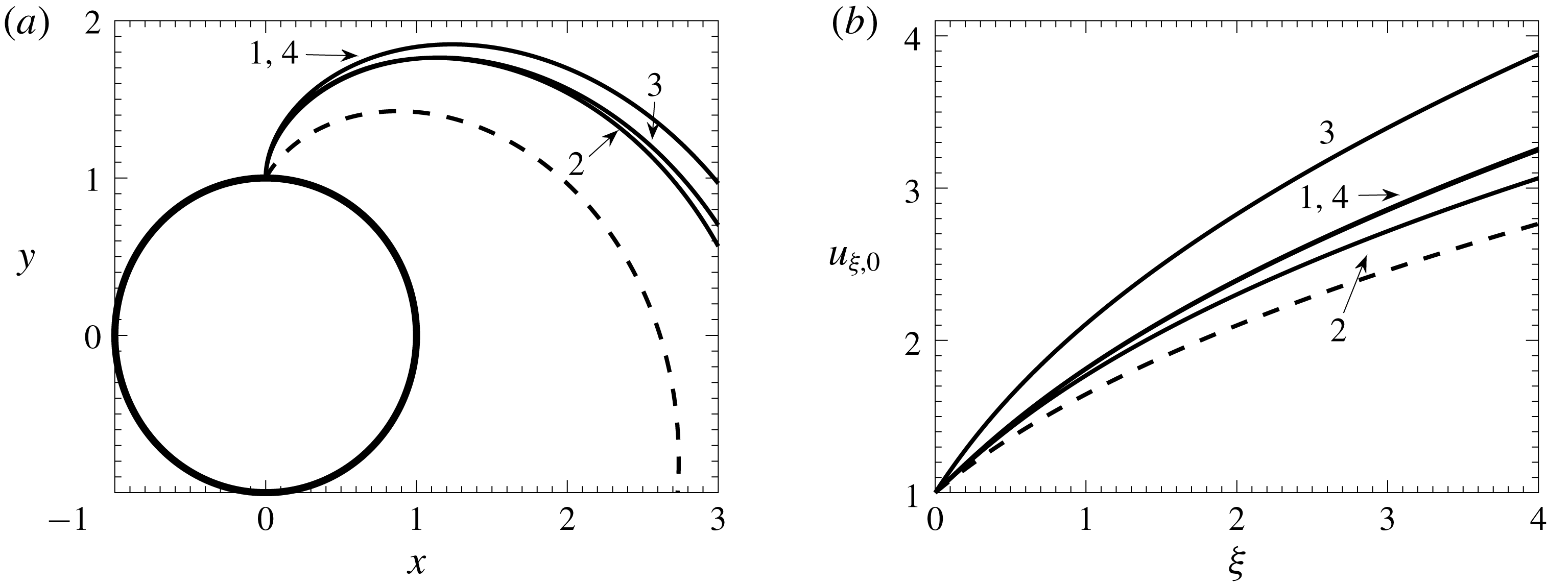
The solution of (3.4)–(3.8) describes the jet’s trajectory, the distribution of the velocity and the jet’s radius along it for the base (unperturbed) flow. In order to find this solution, the system (3.4)–(3.8) must be rearranged into the standard form, i.e. resolved with respect to the highest derivatives, and then integrated numerically using one of the standard methods. In the present study, the fourth-order Runge–Kutta scheme has been used. Some representative trajectories for jets with the initial velocity directed radially and deviating from the radial direction by $30^{\circ }$ are shown in figure 1(a). Figure 1(b) gives the corresponding distributions of the longitudinal components of velocity along the trajectories. Note that, since $Fr\neq \infty$ , the jet’s trajectory does not lie in a plane and figure 1(a) gives the top view of what spatially are helices spiralling out.

Figure 1.

Representative trajectories viewed from above (a) and the corresponding distributions of the component of velocity directed along the jet (b). Curve 1 corresponds to $We=10$ , $Rb=1$ , $Fr=5$ . Variations of the base case 1 are defined as: 2: $We=5$ ; 3: $Rb=0.8$ ; 4: $Fr=2.5$ . The dashed lines show the trajectory and the corresponding velocity distribution for a jet with the velocity at the starting point directed at an angle of $30^{\circ }$ from the radial direction. The solid circle at the bottom of (a) shows the path of the nozzle from which the jet is generated. For all velocities $h_{0}=1/u_{\unicode[STIX]{x1D709},0}^{1/2}$ ; with the velocity and the jet radius scaled by their values at the inlet, $Q_{1}=1$ . Note that the trajectories in (a) do not lie in a plane; spatially, each of them is a helix spiralling out.

Dealing now with perturbations, the continuity equation (2.8) considered at $O(\unicode[STIX]{x1D6FF}\unicode[STIX]{x1D716}^{-1})$ as $\unicode[STIX]{x1D716}\rightarrow 0$ gives

(3.9) $$\begin{eqnarray}\frac{\unicode[STIX]{x2202}\tilde{u} _{\unicode[STIX]{x1D709}}}{\unicode[STIX]{x2202}\unicode[STIX]{x1D709}_{0}}+\frac{\unicode[STIX]{x2202}\tilde{u} _{\unicode[STIX]{x1D702}}}{\unicode[STIX]{x2202}\unicode[STIX]{x1D702}}+\frac{\tilde{u} _{\unicode[STIX]{x1D702}}}{\unicode[STIX]{x1D702}}=0.\end{eqnarray}$$

This equation may be integrated with respect to $\unicode[STIX]{x1D702}$ , given that $\tilde{u} _{\unicode[STIX]{x1D709}}$ is assumed to be independent of $\unicode[STIX]{x1D702}$ , to obtain

(3.10) $$\begin{eqnarray}\tilde{u} _{\unicode[STIX]{x1D702}}=-\frac{\unicode[STIX]{x1D702}}{2}\frac{\unicode[STIX]{x2202}\tilde{u} _{\unicode[STIX]{x1D709}}}{\unicode[STIX]{x2202}\unicode[STIX]{x1D709}_{0}},\end{eqnarray}$$

which is similar to (3.8) for the base flow. Using this in the kinematic condition (2.16) at $O(\unicode[STIX]{x1D6FF}\unicode[STIX]{x1D716}^{-1})$ as $\unicode[STIX]{x1D716}\rightarrow 0$ , the equation

(3.11) $$\begin{eqnarray}\frac{\unicode[STIX]{x2202}\tilde{h}}{\unicode[STIX]{x2202}t_{0}}+u_{\unicode[STIX]{x1D709},0}\frac{\unicode[STIX]{x2202}\tilde{h}}{\unicode[STIX]{x2202}\unicode[STIX]{x1D709}_{0}}+\frac{h_{0}}{2}\frac{\unicode[STIX]{x2202}\tilde{u} _{\unicode[STIX]{x1D709}}}{\unicode[STIX]{x2202}\unicode[STIX]{x1D709}_{0}}=0\end{eqnarray}$$

is obtained, where $u_{\unicode[STIX]{x1D709},0}$ is evaluated at $\unicode[STIX]{x1D709}_{1}=0$ , i.e.  $\unicode[STIX]{x1D709}=\unicode[STIX]{x1D709}_{a}$ .

Equations (2.13), (2.14) to order $O(\unicode[STIX]{x1D6FF}\unicode[STIX]{x1D716}^{-1})$ as $\unicode[STIX]{x1D716}\rightarrow 0$ give that $\tilde{p}$ is independent of $\unicode[STIX]{x1D702}$ and $\unicode[STIX]{x1D703}$ , i.e. uniform across the cross-section. Then, using that from (3.3)

(3.12) $$\begin{eqnarray}\tilde{p}=-\frac{\tilde{h}}{h_{0}^{2}}-\frac{\unicode[STIX]{x2202}^{2}\tilde{h}}{\unicode[STIX]{x2202}\unicode[STIX]{x1D709}_{0}^{2}},\end{eqnarray}$$

equation (2.12) to the same order yields

(3.13) $$\begin{eqnarray}\frac{\unicode[STIX]{x2202}\tilde{u} _{\unicode[STIX]{x1D709}}}{\unicode[STIX]{x2202}t_{0}}+u_{\unicode[STIX]{x1D709},0}\frac{\unicode[STIX]{x2202}\tilde{u} _{\unicode[STIX]{x1D709}}}{\unicode[STIX]{x2202}\unicode[STIX]{x1D709}_{0}}-\frac{1}{We}\left(\frac{1}{h_{0}^{2}}\frac{\unicode[STIX]{x2202}\tilde{h}}{\unicode[STIX]{x2202}\unicode[STIX]{x1D709}_{0}}+\frac{\unicode[STIX]{x2202}^{3}\tilde{h}}{\unicode[STIX]{x2202}\unicode[STIX]{x1D709}_{0}^{3}}\right)=0.\end{eqnarray}$$

Substituting

(3.14) $$\begin{eqnarray}(\tilde{u} _{\unicode[STIX]{x1D709}},\tilde{h})=(A_{u},A_{h})\text{e}^{\text{i}(k\unicode[STIX]{x1D709}_{0}-\unicode[STIX]{x1D714}t_{0})},\end{eqnarray}$$

where $A_{u}$ , $A_{h}$ are amplitudes, $k$ is the wavenumber and $\unicode[STIX]{x1D714}$ is the frequency, into (3.11), (3.13), the following system is obtained:

(3.15) $$\begin{eqnarray}\displaystyle & \displaystyle (ku_{\unicode[STIX]{x1D709},0}-\unicode[STIX]{x1D714})A_{h}+\frac{kh_{0}}{2}A_{u}=0, & \displaystyle\end{eqnarray}$$

(3.16) $$\begin{eqnarray}\displaystyle & \displaystyle \frac{k}{We}\left(k^{2}-\frac{1}{h_{0}^{2}}\right)A_{h}+\left(ku_{\unicode[STIX]{x1D709},0}-\unicode[STIX]{x1D714}\right)A_{u}=0. & \displaystyle\end{eqnarray}$$

This system of equations has a non-trivial solution only if

(3.17) $$\begin{eqnarray}(ku_{\unicode[STIX]{x1D709},0}-\unicode[STIX]{x1D714})^{2}-\frac{k^{2}}{2Weh_{0}}(h_{0}^{2}k^{2}-1)=0,\end{eqnarray}$$

which is the dispersion equation for the waves in question. This equation is completely analogous to (2.17) of Le Dizès & Villermaux (Reference Le Dizès and Villermaux2017) apart from the viscous term accounted for in the latter. It should be remembered though that the base flow characteristics, $u_{\unicode[STIX]{x1D709},0}$ and $h_{0}$ , vary along the jet differently, since for the case considered here, they come from solving (3.4)–(3.8). In particular, although the dispersion equation (3.17) depends only on $We$ , the base flow variables, $u_{\unicode[STIX]{x1D709},0}$ and $h_{0}$ , depend also on $Fr$ and $Rb$ .

In applications of rotating jets, the disturbances are introduced mainly at the starting point of the jet, the orifice or the edge of a spinning disc, where the jet is subjected to vibrations of the spinning device. It is this situation that is of interest here. Therefore, $\unicode[STIX]{x1D714}$ in (3.17) is considered to be the frequency of the wave that is spatially the fastest growing one corresponding to the base flow at the start of the jet. The evolution of this wave down the jet is followed until the nonlinear regime to see what drops will be produced as a result.

Considering $\unicode[STIX]{x1D714}$ in (3.17) as real and the wavenumber $k$ as complex, $k=k_{r}+\text{i}k_{i}$ , equation (3.17) can be split into real and imaginary parts:

(3.18) $$\begin{eqnarray}\left.\begin{array}{@{}c@{}}\displaystyle (k_{r}u_{\unicode[STIX]{x1D709},0}-\unicode[STIX]{x1D714})^{2}-(k_{i}u_{\unicode[STIX]{x1D709},0})^{2}-\frac{1}{2Weh_{0}}[h_{0}^{2}((k_{r}^{2}-k_{i}^{2})^{2}-(2k_{r}k_{i})^{2})-(k_{r}^{2}-k_{i}^{2})]=0,\\ \displaystyle 2k_{i}u_{\unicode[STIX]{x1D709},0}(k_{r}u_{\unicode[STIX]{x1D709},0}-\unicode[STIX]{x1D714})-\frac{1}{Weh_{0}}[2k_{r}k_{i}h_{0}^{2}(k_{r}^{2}-k_{i}^{2})-k_{r}k_{i}]=0,\end{array}\right\}\end{eqnarray}$$

where the last equation, after dividing it by $k_{r}k_{i}\neq 0$ and rearranging, takes the form

(3.19) $$\begin{eqnarray}k_{i}^{2}=k_{r}^{2}-\frac{1}{2h_{0}^{2}}\left[2Weh_{0}u_{\unicode[STIX]{x1D709},0}\left(u_{\unicode[STIX]{x1D709},0}-\frac{\unicode[STIX]{x1D714}}{k_{r}}\right)+1\right].\end{eqnarray}$$

The frequency $\unicode[STIX]{x1D714}_{ini}$ , for which $k_{i}<0$ has its minimum, is the slender-jet analogue of the Rayleigh frequency; the corresponding real part, $k_{r}$ , will then determine the wavelength of the propagating disturbance.

The amplitude of the initially generated wave increases as the wave propagates down the jet. Eventually, the jet dynamics enters the nonlinear regime where the amplitude of the wave is no longer small so that the viscous effects have to be taken into account. The distance from the starting point of the jet to the region where the jet’s dynamics becomes essentially nonlinear depends on the amplitude of the disturbance at the inlet. In practical applications, this amplitude is not known. Therefore, instead of calculating the gain in the amplitude of the wave in the linear regime from its unknown initial value, as in Le Dizès & Villermaux (Reference Le Dizès and Villermaux2017), the initial magnitude of the wave is taken as a free parameter characterized implicitly by the distance from the starting point of the jet to the point where the jet breaks up. The conventional boundary between the regions of small and finite-amplitude perturbations and the amplitude of the perturbations at this boundary become parameters linked by the constraint that the distance to the point of the jet breakup remains the same for the same case.

Note that the above picture of the propagating and spatially growing waves corresponds to convective instability which takes place for the Weber number above a certain critical value. This critical Weber number in the case of a straight jet is known to be $We=3.15$ for inviscid flow (Leib & Goldstein Reference Leib and Goldstein1986b ) and lower for viscous flow (Leib & Goldstein Reference Leib and Goldstein1986a ), with the value depending on the Reynolds number. In the calculations below, as for the trajectories given above, the Weber number is taken to be above the critical value; the Reynolds number needed to characterize the flow in the nonlinear regime is introduced below.

4 Finite-amplitude waves and formation of drops

Consider how convective instability develops, i.e. how the wave generated at the start of the jet, with the frequency corresponding to the fastest spatially growing wave at this point, will evolve and lead to drop formation. This section focuses on the regular regime of drop generation, with the drops reproducibly emitted from the jet’s end, and the initial conditions used to start the calculations play no role anymore. A representative case is studied where a jet with a circular cross-section is generated at a distance $L$ from the axis of rotation (the distance used as the characteristic length scale for non-dimensionalization) with the velocity at the onset of the jet directed radially.

Using the initial velocity $U$ and the initial radius of the jet $H$ as the scales for the longitudinal velocity and the cross-sectional length, respectively, the base case $We=10$ , $Rb=1$ , $Fr=5$ is considered and, to illustrate the influence of the flow parameters, variations from these values as in figure 1, i.e.  $We=5$ , $Rb=0.8$ and $Fr=2.5$ , are used. For the slender-jet approximation and hence the equations for $k_{r}$ and $k_{i}$ to be applicable, it is necessary that $\unicode[STIX]{x1D716}=H/L\ll 1$ . Expressing $H$ , $L$ and $U$ in terms of the non-dimensional parameters as

(4.1a-d ) $$\begin{eqnarray}H=\frac{\unicode[STIX]{x1D70E}We}{\unicode[STIX]{x1D70C}U^{2}}=\frac{\unicode[STIX]{x1D70E}We\unicode[STIX]{x1D6FA}^{2}Rb^{2}}{\unicode[STIX]{x1D70C}g^{2}Fr^{4}},\quad L=\frac{Fr^{2}}{Rb^{2}}\frac{g}{\unicode[STIX]{x1D6FA}^{2}},\quad U=\unicode[STIX]{x1D6FA}RbL=\frac{Fr^{2}}{Rb}\frac{g}{\unicode[STIX]{x1D6FA}},\end{eqnarray}$$

the condition for the applicability of the slender-jet approximation takes the form

(4.2) $$\begin{eqnarray}\unicode[STIX]{x1D716}=\frac{H}{L}=\frac{\unicode[STIX]{x1D70E}\unicode[STIX]{x1D6FA}^{4}}{\unicode[STIX]{x1D70C}g^{3}}\frac{WeRb^{4}}{Fr^{6}}\ll 1.\end{eqnarray}$$

For the base case ( $We=10$ , $Rb=1$ , $Fr=5$ ) and the values of the dimensional parameters in a typical experiment ( $\unicode[STIX]{x1D6FA}=150~\text{s}^{-1}$ , $\unicode[STIX]{x1D70E}=50~\text{dyn}~\text{cm}^{-1}$ , $\unicode[STIX]{x1D70C}=1$ $\text{g}~\text{cm}^{-3}$ , $g=981~\text{cm}~\text{s}^{-2}$ ), it follows that $\unicode[STIX]{x1D716}\approx 0.017$ .

The dispersion equation (3.17) depends on $u_{\unicode[STIX]{x1D709},0}$ , $h_{0}=1/\sqrt{u_{\unicode[STIX]{x1D709},0}}$ and $We$ ; then the non-dimensional frequencies of the spatially fastest growing disturbance at the onset of the jet ( $u_{\unicode[STIX]{x1D709},0}=1$ , $h_{0}=1$ ) for $We=10$ and $We=5$ are $\unicode[STIX]{x1D714}_{ini}=0.736$ and $\unicode[STIX]{x1D714}_{ini}=0.774$ , respectively.

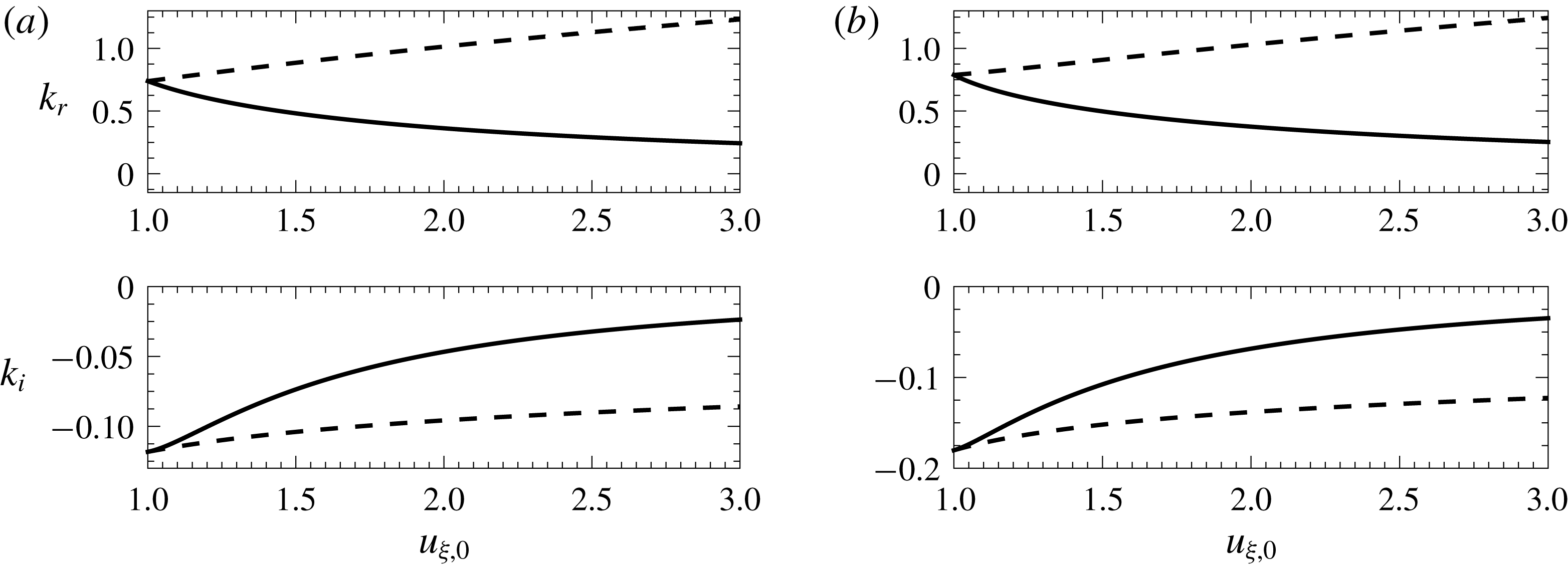
With the value of $\unicode[STIX]{x1D714}_{ini}$ fixed, the evolution of $k_{r}$ and $k_{i}$ corresponding to this value may be considered along the jet for the linear regime of the wave propagation. These distributions as functions of the base velocity $u_{\unicode[STIX]{x1D709},0}$ are shown in figure 2; the dependence on $\unicode[STIX]{x1D709}$ can then be obtained by combining these curves with the distributions of the longitudinal velocity along the jet shown in figure 1(b).

Figure 2.

The dependence of $k_{r}$ and $k_{i}$ on the longitudinal velocity of the base flow, $u_{\unicode[STIX]{x1D709},0}$ . (a) $We=10$ ; (b) $We=5$ . The dashed lines show $k_{r}$ and $k_{i}$ corresponding to the local analogue of the Rayleigh wave.

As the perturbations introduced at the starting point of the jet propagate along the jet, their amplitude grows and gradually they enter the nonlinear stage of evolution. Then, in addition to capillarity and inertia, it becomes necessary to take into account the fluid’s viscosity and hence add to the set of parameters characterizing the flow the Reynolds number, defined using the inlet parameters, $Re=\unicode[STIX]{x1D70C}UH/\unicode[STIX]{x1D707}$ .

To match the small-amplitude wave treated as the linear solution close to the jet’s starting point with the finite-amplitude nonlinear numerical solution further down the jet, an artificial boundary between the two regions is introduced, which is a cross-section where, using the known linear solution, the boundary conditions for the nonlinear one are set. This boundary is characterized by its distance from the starting point of the jet and the amplitude of the wave at this cross-section. These two parameters can be varied to ensure that the results, notably the distance from the start of the jet to the point where the drop is produced and the drop’s volume, are independent of the boundary’s location. In particular, this means that the ‘end code’ which is used to describe the nonlinear stage of the wave’s evolution takes the solution where the flow is yet in the linear regime and the effects of viscosity are negligible. In other words, a smaller-amplitude linear wave set as the boundary conditions at the matching boundary located closer to the starting point of the jet, and a larger-amplitude wave set at the matching boundary located further down the jet, correspond to the same initial disturbance if they produce the same drops at the same distance from the jet’s starting point. This simple check ensures that the flow between the two matching boundaries is accurately described by the linear solution, i.e. the wave amplitude is ‘small’ and the effect of viscosity is negligible. The nonlinear regime of the wave’s evolution was studied using the ‘end code’ based on the finite-element method; the code has been developed as an appropriate modification of the code used earlier (Li & Sprittles Reference Li and Sprittles2016).

The code uses an arbitrary Lagrangian–Eulerian approach, known as the method of spines and described in detail in Kistler & Scriven (Reference Kistler and Scriven1984), so that the free-surface dynamics is captured with high accuracy. The structured mesh with triangular elements uses a quadratic approximation for velocity and a linear approximation for pressure to satisfy the Ladyzenskaya–Babuska–Brezzi condition (Aziz Reference Aziz1972). The main development compared with Li & Sprittles (Reference Li and Sprittles2016) is the re-meshing algorithm which increases the mesh density as the free surface slope increases and the jet approaches the breakup and reduces it as the jet recovers after the breakup before the next cycle of drop generation starts. This algorithm considerably reduces the computational time whilst maintaining the computational accuracy.

At the cross-section separating the linear and the nonlinear regimes, for a given $\unicode[STIX]{x1D714}=\unicode[STIX]{x1D714}_{ini}$ the wavenumber $k$ is known from the dispersion equation (3.17) and, after prescribing, for example, the amplitude of the free-surface oscillations $A_{h}$ , the amplitude and phase of the velocity oscillations $A_{u}$ can be found from one of (3.15), (3.16). Then, using (3.14) with $\unicode[STIX]{x1D6FF}$ absorbed into $A_{u}$ , the longitudinal velocity can be prescribed as $u_{\unicode[STIX]{x1D709},0}+\tilde{u} _{\unicode[STIX]{x1D709}}$ . The radial component of velocity, needed as the ‘end code’ accounts for the fluid’s viscosity, is then given by (3.10). These boundary conditions, once fed into the ‘end code’ describing the bulk flow, make it possible to compute how the drops form. Note that, although the two parameters characterizing the linear–nonlinear boundary (the location and amplitude $A_{h}$ ) can be varied independently (subject to the constraints outlined above), the physical process itself has only one degree of freedom, namely the magnitude of the initial disturbance introduced at the start of the jet. In practice, the amplitude associated with vibrations of the jet-producing device is usually difficult to determine, and it is more convenient to characterize the solutions not by this amplitude but by looking at the process ‘from the other end’, using the easily measurable distance $\unicode[STIX]{x1D709}_{b}$ from the starting point of the jet to the point where the drops break away from the rest of the jet.

Figure 3.

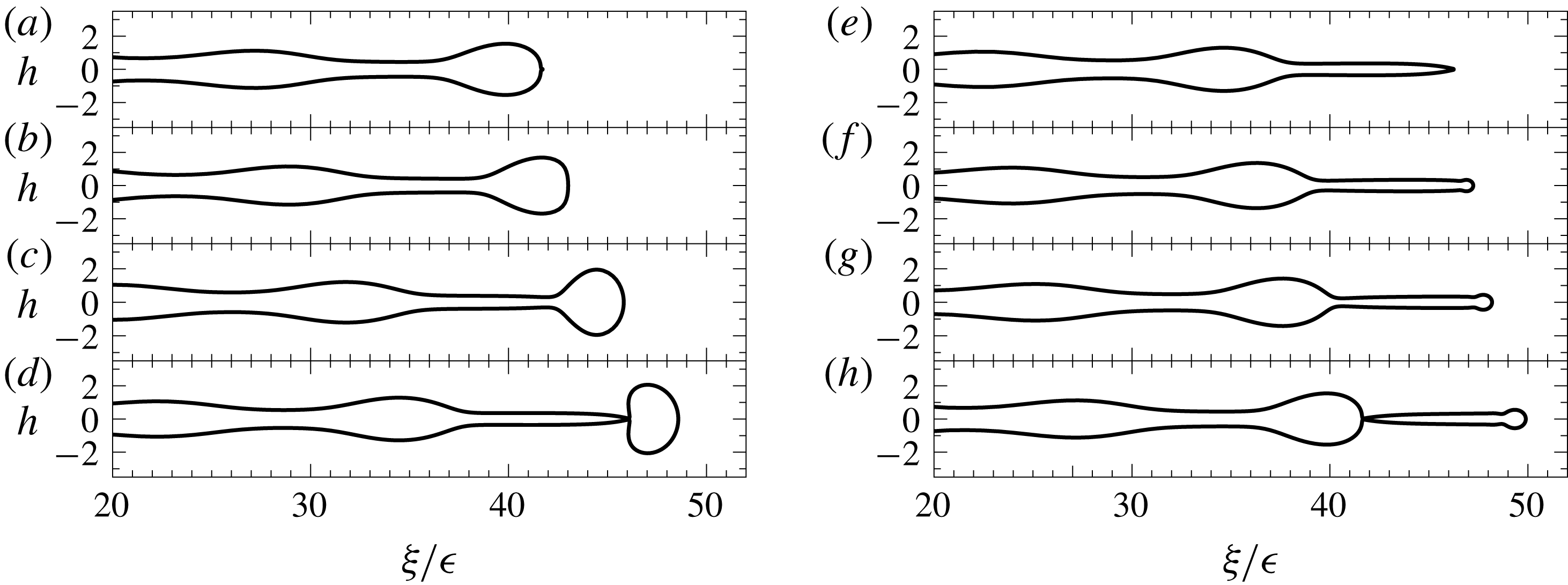
The evolution of the free-surface profile for the case where the ‘end code’ considers the jet’s dynamics from the outset, i.e. from $u_{\unicode[STIX]{x1D709},0}=1$ with $A_{h}=0.04$ . Frames (a–d) describe the formation of the main drop and correspond to $t=0$ , $1.7$ , $3.3$ , $5.0$ , respectively; frames (e–h) show the formation of the satellite droplets and correspond to $t=5.0$ , $6.1$ , $7.3$ , $8.5$ , respectively (the time is measured from the beginning of the cycle). The pinch-off point of the main drop is located at a distance of about $46$ times the initial jet radius. $We=10$ , $Rb=1$ , $Fr=5$ , $Re=50$ , $\unicode[STIX]{x1D716}=0.0172$ .

Figure 4.

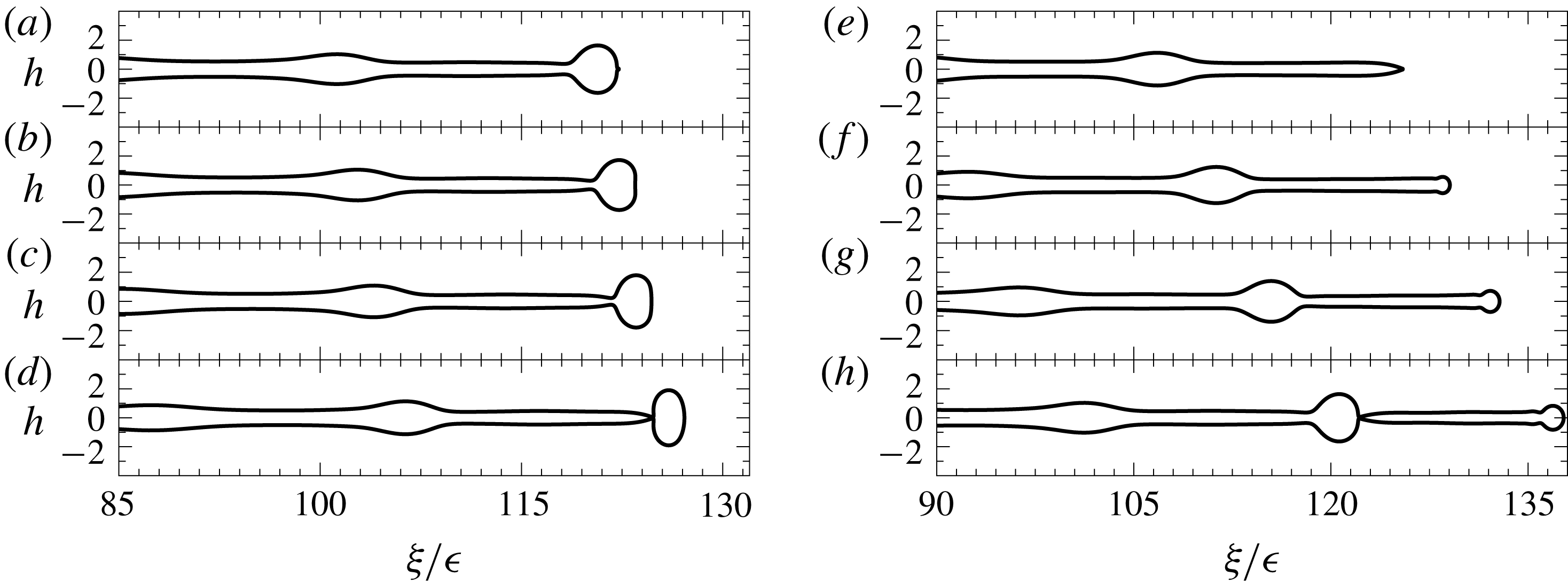
The evolution of the free-surface profile for the case where the ‘end code’ is used from $u_{\unicode[STIX]{x1D709},0}=1.7$ with $A_{h}=0.04$ . Frames (a–d) describe the formation of the main drop and correspond to $t=0$ , $0.8$ , $1.6$ , $2.4$ , respectively; frames (e–h) show the formation of the satellite droplet and correspond to $t=2.4$ , $4.4$ , $6.5$ , $8.5$ , respectively. The main drop breaks away at a distance of approximately $124$ times the initial jet radius.

As mentioned in § 1, the exact computation of the nonlinear regime of evolution of a curved jet would require resolving widely disparate length scales in a three-dimensional unsteady free-boundary problem which is beyond what available computational resources allow, especially for the regular regime of the drop generation.

To make calculations feasible, an approximation actually employing the disparity of the length scales and the known/computed trajectory may be used to reduce the dimensionality of the problem as follows. The spiralling shape of the jet’s trajectory influences the flow dynamics in two ways. Firstly, the role of stretching the jet played by the gravity force in the case of a straight jet (Le Dizès & Villermaux Reference Le Dizès and Villermaux2017) is played by the projections of the centrifugal force and the gravity force on the jet’s trajectory in the case of the spiralling jet. These projections depend on the shape of the trajectory and vary along it. Then, given that the jet’s trajectory has been found, the effect of this factor can be captured by projecting the centrifugal force and the gravity force onto the known trajectory and using them as the external body forces acting along a straight jet. In other words, instead of a constant gravity force acting along a straight jet, the prescribed spatial variation of body force (calculated as described above) acting along a straight jet can be used to model the stretching effect that the centrifugal and gravity forces have on the spiralling jet. Secondly, the free-surface curvature deviates from axial symmetry with regard to the jet’s centreline affecting the base flow accordingly. This effect in the slender-jet regime is of $O(\unicode[STIX]{x1D716})$ as $\unicode[STIX]{x1D716}\rightarrow 0$ . Note that the terms of $O(\unicode[STIX]{x1D716})$ in (3.3) have been fully accounted for in calculating the trajectory (Shikhmurzaev & Sisoev Reference Shikhmurzaev and Sisoev2017). Thus, an a priori estimate of the accuracy is $O(\unicode[STIX]{x1D716})$ if (a) the flow in the spiralling jet is computed using, as the external body force, the projection of the centrifugal and gravity forces onto the jet’s trajectory and (b) the expression for the full curvature of a straight jet is used. This approximation tested a posteriori against the full-scale three-dimensional unsteady code for jets where such computations were feasible appears to be surprisingly accurate, well within the computational accuracy of both codes. Both codes use the finite-element method; the code implementing the approximation outlined above is a modified version of the code used in Li & Sprittles (Reference Li and Sprittles2016).

Figures 3 and 4 show the evolution of the free-surface profile with the matching boundary between the linear and nonlinear dynamics located at different distances from the starting point, and the same amplitude of the wave at this point. In other words, these plots correspond to different magnitude of disturbances at the inlet and hence different distances to the breakup point, $\unicode[STIX]{x1D709}_{b}$ . In figure 3, the ‘end code’ is attached straight to the inlet, i.e. starts from $u_{\unicode[STIX]{x1D709},0}=1$ , and $A_{u}=0.04$ . Figure 4 corresponds to $u_{\unicode[STIX]{x1D709},0}=1.7$ and $A_{h}=0.04$ at the matching boundary. Frames (a–d) of each figure show the formation of the main drop; frames (e–h) describe the detachment of the satellite droplet. It should be noted here that the ‘primary’ satellite shown in the figures, if sufficiently long, potentially can undergo further breakup which is not studied here. The full cycle, which includes the formation of the main drop and the primary satellite, corresponds to the period of the initial excitation.

Qualitatively, the formation of the main and the satellite drop is broadly the same as in the dripping process, as described originally by Lenard (Reference Lenard1887) and then studied in detail in many works, notably Ambravaneswaran et al. (Reference Ambravaneswaran, Phillips and Basaran2000), Chakraborty et al. (Reference Chakraborty, Rubio-Rubio, Sevilla and Gordillo2016) and Borthakur et al. (Reference Borthakur, Biswas and Bandyopadhyay2017); see also references therein and in Shikhmurzaev (Reference Shikhmurzaev2007, Ch. 7). At the same time, there are several features indicating a different balance of physical factors. As figures 3 and 4 show, unlike slow dripping, where the frontal side of the main drop is almost spherical throughout the process of drop formation and detachment, the process is more dynamic and the tip almost flattens as it recoils after the detachment of the satellite. Another characteristic feature is that, as seen in frames (e–h) of both figures, the bulge on the jet takes the shape of the future main drop while the satellite is still forming before breaking away, and the subsequent pinch-off of the neck connecting the main drop with the jet is assisted by the recoil of the forming drop driven by the capillary pressure due to the curvature of its frontal side. It is also worth pointing out that, in the regular regime of drop generation, the value of $\unicode[STIX]{x1D709}_{b}$ for the satellite droplet is slightly smaller than $\unicode[STIX]{x1D709}_{b}$ for the main drop.

Comparing figures 3 and 4, it is seen that, whilst the whole cycle where the main drop and the satellite droplet are produced remains the same (within the computational accuracy), the proportion of time taken by the main drop and the satellite droplet to form and detach depends on how far down the jet this happens. It can be said that globally the whole process is, in a certain sense, linear, with the global periodicity controlled by the linear regime, whilst the nonlinearity of the drop formation is in this sense local, i.e. manifesting itself in the local dynamics as the breakup itself is approached within the globally preset cycle. The shortening of the time for the main drop to form and detach can be attributed to the fact that its detachment is assisted by the recoil of the forming drop after emitting the satellite, and, as the jet gets thinner down the trajectory, the capillary pressure at the drop’s frontal side which leads to an increase in the recoil velocity. By contrast, the satellite droplet is produced out of a stretched ligament and, as can be seen in figures 3 and 4, its detachment from the main body of the jet happens long before the recoiling end generates an appreciable wave along it. It should be noted that the proportion of the liquid’s volume that goes into the main drop and the satellite droplet also varies along the jet.

Figure 5.

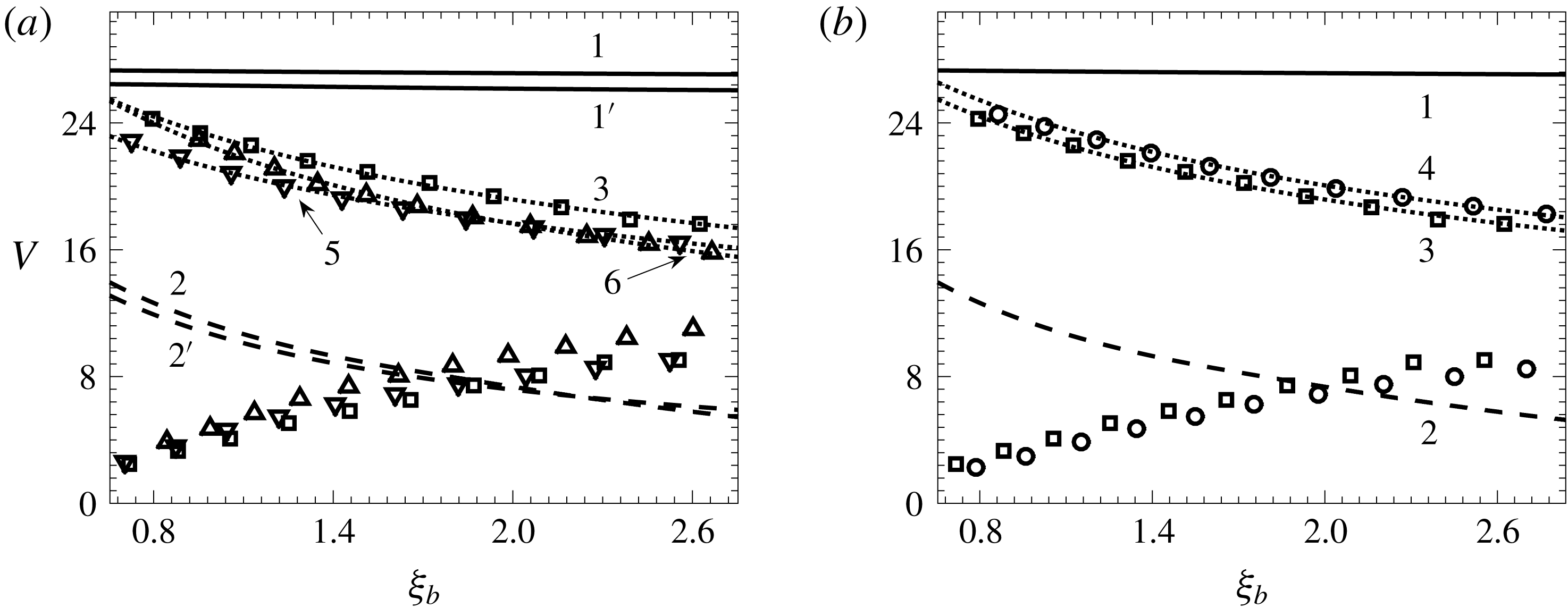
Dependence of the volumes of the main drop (upper markers) and the satellite droplet (lower markers) on the distance, $\unicode[STIX]{x1D709}_{b}$ , of their appearance measured from the starting point of the jet for different $We$ , $Rb$ and $Re$ . (▫)  $We=10$ , $Rb=1$ , $Fr=5$ , $Re=50$ (base case); (▿) $We=5$ ; (▵) $Rb=0.8$ ; (○) $Re=25$ . Solid lines $1$ and $1^{\prime }$ show the volume of fluid contained within one wavelength obtained from the dispersion equation (3.17) with initial frequency $\unicode[STIX]{x1D714}_{ini}$ for $We=10$ and $We=5$ , respectively; this volume is equal to the sum of the volumes of the main and satellite drops. Dashed lines $2$ and $2^{\prime }$ correspond to the volumes of fluid contained within one wavelength of the locally most unstable wave, i.e. the local Rayleigh volume obtained from (3.17) with the frequency of the fastest growing wave, for $We=10$ and $We=5$ , respectively; this volume is proportional to $h_{0}^{3}$ . Curves 3–6 (dotted lines) are the linear fits $V=C_{1}h_{0}(\unicode[STIX]{x1D709}_{b})+C_{2}$ with the following parameters: (3) $C_{1}=45.1$ , $C_{2}=-7.7$ ; (4) $C_{1}=42.6$ , $C_{2}=-7.5$ ; (5) $C_{1}=37.3$ , $C_{2}=-6.9$ ; (6) $C_{1}=50.8$ , $C_{2}=-12.6$ .

This last feature is illustrated in figure 5 showing how the volumes of the main drops and the satellite droplets depend on the distance along the jet where they are produced. The volume of the fluid contained within one wavelength is the sum of volumes of the main drop and the primary satellite, whilst the size of the main drop decreases as a linear function of the radius of the unperturbed jet evaluated at the point of breakup. The linear fits

(4.3) $$\begin{eqnarray}V(\unicode[STIX]{x1D709}_{b})=C_{1}h_{0}(\unicode[STIX]{x1D709}_{b})+C_{2}\end{eqnarray}$$

are shown as the dotted lines in figure 5 with the values of the fitting parameters given in the figure caption. This last feature indicates that an estimate for the size of the main drop based on the linear theory without considering the nonlinear dynamics of the jet’s breakup becomes increasingly inaccurate the further away one gets from the jet’s starting point. As one can also see in figure 5, the prediction based on the local Rayleigh instability is far from the computed results. This is in fact what one should expect in the case of incident excitation, and this feature could be used in the analysis of experiments to identify the dominant source of disturbances.

The computed data shown in figure 5 for different values of parameters correspond to the same starting points of the ‘end code’, namely $u_{\unicode[STIX]{x1D709},0}=1$ , $1.1$ , $1.2$ , $1.3$ , $1.4$ , $1.5$ , $1.6$ , $1.7$ , $1.8$ , $1.9$ , and the same amplitude $A_{h}=0.04$ at this point. The influence of the parameters on the breakup distance can also be seen. In particular, higher viscosity increases the breakup distance and leads to marginally larger drops being produced. It should be noted also that as the volumes of the main and the satellite drops become closer, the free-surface shape becomes more and more complicated making it necessary to increase the spatial resolution of the code.

The gradual convergence of the volumes of the main and satellite drops can be seen in figure 5. This may suggest revisiting the results obtained by Rutland & Jameson (Reference Rutland and Jameson1970), who found in their pressurized dripping experiment that, despite their theoretical expectations, the satellite drops are always present and conjectured that uniformity of the drop sizes could be achieved once the satellites reach the size of the main drop. Whether this is indeed possible remains an open question as the nonlinear dynamics of the jet as it approaches breakup becomes increasingly complex as its cross-sectional dimension decreases (Castrejón-Pita et al. Reference Castrejón-Pita, Castrejón-Pita, Thete, Sambath, Hitchings, Hinch, Lister and Basaran2015).

5 Concluding remarks

The analysis of the linear regime of propagation of disturbances generated at the onset of a jet produced by a spinning device is qualitatively similar to that in the case of a straight jet stretched by gravity (Le Dizès & Villermaux Reference Le Dizès and Villermaux2017) with the dispersion equation (3.17) having the same parametric dependence on the base flow. However, the linear regime gives insufficient information about the size of the drops to be produced, and the numerical analysis of the nonlinear dynamics of the drop formation shows that the wavelength of the initial excitation, increasing as the wave propagates down the stretching jet, determines not the volume of the drops produced but the total volume of the main drop and the satellite droplet that follows the main one. A feature potentially important for practical applications is that the volume of the main drop, $V$ , can be accurately approximated by a linear dependence (4.3) of $V$ on the unperturbed radius of the jet, $h_{0}$ , evaluated at the breakup point. Notably, not only the share of the total volume of the fluid contained within one wavelength that forms the main drop but also the share of the time it takes for each of them to develop depend on where along the jet the drops are produced.

The drop formation process is very complex, starting from linear disturbances propagating down the jet which soon enter a nonlinear regime, eventually culminating in the pinch-off of the main drop followed by the recoil of the jet’s tip and the pinch-off of the satellite droplet. This level of complexity requires a consistent multiple-scales analysis of the linear stage and a careful numerical simulation of the much more intricate nonlinear regime and the topological transition. An attempt to predict the outcome on the basis of a linear analysis stands a very small chance of success. For example, Wallwork et al. (Reference Wallwork, Decent, King and Schulkes2002) applied the local linear analysis to estimate the breakup length by equating the amplitude of a linear (exponential) wave to the radius of the jet, i.e. stretching the linear regime to the breakup. Unsurprisingly, it was found that the breakup length obtained in this way disagrees with the authors’ own experimental data, and the discrepancy was attributed, quite plausibly, to their ‘using a linear theory while the breakup mechanism is a nonlinear effect’ as well as to the jet’s trajectory not lying in a plane as was assumed in their theory. However, in subsequent works (Decent, King & Wallwork Reference Decent, King and Wallwork2002; Decent et al. Reference Decent, King, Simmons, Părău, Wallwork, Gurney and Uddin2009) the same linear approach was used to estimate the volumes of the main drop and even of the satellite droplet, though in Wallwork et al. (Reference Wallwork, Decent, King and Schulkes2002) the reader was cautioned that the satellite droplets ‘are not predicted by the linear theory as they are a nonlinear effect’. Nevertheless, in a follow-up paper, the small size of the satellite droplets is explained using the linear theory: ‘shorter waves become unstable which could produce satellite drops’ (Decent et al. Reference Decent, King, Simmons, Părău, Wallwork, Gurney and Uddin2009, p. 4295). As the results of the numerical simulations in the present study show, the linear analysis is inadequate for describing the nonlinear stage of wave propagation as well as drop formation, and, as for the satellite droplets, they result from the pinch-off of a long thin ligament connecting the main drops, not from short waves, which may be considered in the linear stage of the wave propagation. This is what can be seen in the experimental photographs of Wallwork et al. (Reference Wallwork, Decent, King and Schulkes2002) as well as in numerous experimental studies of particular atomization systems (see Li et al. Reference Li, Sisoev and Shikhmurzaev2018 for a recent overview of the most non-trivial one).

Finally, we draw attention to one rather non-trivial aspect of the use of the linear analysis. Strictly speaking, the linear analysis is applicable to waves of an infinitesimal amplitude whilst, in practice, its results are applied to describe waves of a small but finite amplitude. Not an issue for spatially uniform jets, this point becomes non-trivial when it comes to jets with a spatially varying base flow, like the jets driven by gravity or the jets spiralling out under the action of the centrifugal force considered here. Then, for the relatively short jets of the kind that can be typically encountered in practical applications, i.e. if the amplitude of disturbances at the outlet is ‘not too small’, it is the initially fastest spatially growing wave that transitions to the nonlinear regime and ultimately determines the subsequent nonlinear dynamics and its outcome (the drops produced). However, for ‘very small’ disturbances at the outset (and, consequently, very long jets), the initially fastest growing wave could become increasingly irrelevant before it reaches an appreciable amplitude and its role could be taken over by the fastest growing waves corresponding to the points further down the jet. This would require using at the linear stage the maximum-net-gain approach developed by Le Dizès & Villermaux (Reference Le Dizès and Villermaux2017). The results presented here, which come from the combination of the linear analysis and numerical simulations of the nonlinear regime, where the location of the linear–nonlinear interface is varied, show that for waves with an initial amplitude (in terms of the jet’s radius variation) of 0.01 or larger, the initially fastest spatially growing wave approach can be relied upon. Interestingly, this approach appears to be working even when applied to the spinning disc atomization process (Li et al. Reference Li, Sisoev and Shikhmurzaev2018), where, pictorially, there is no well-defined ‘starting point of the jet’ as it has to be determined from the dynamic properties of the gradually forming jet.