1 Introduction
The transport of heat or mass in disperse multiphase systems is a problem both of fundamental and practical interest. Several industrial applications involve flows with suspended particles or drops undergoing chemical reactions, leading to transport across an interface. In suspension polymerization (Vivaldo-Lima et al. Reference Vivaldo-Lima, Wood, Hamielec and Penlidis1997; Brooks Reference Brooks2010), initial monomer drops transform to solid particles, and the exothermic polymerization leading to this transformation necessitates the efficient removal of heat by convection. A second problem is the vaporization of atomized fuel jets, in a turbulent ambient, in internal combustion engines (Law Reference Law1982) which may have a direct impact on efficiency and emission levels. Phenomena in nature, such as cloud formation, entailing condensation in an ambient turbulent flow, also involve the transfer of heat from and mass to water drops (Kinzer & Gunn Reference Kinzer and Gunn1951; Beard & Pruppacher Reference Beard and Pruppacher1971; Duguid & Stampfer Jr Reference Duguid and Stampfer1971). The transport from particles or drops is also relevant in biological systems where the uptake of nutrients and other biochemicals by cells in complex flows is of interest (Magar, Goto & Pedley Reference Magar, Goto and Pedley2003; Guasto, Rusconi & Stocker Reference Guasto, Rusconi and Stocker2012; Stocker Reference Stocker2012).
In this paper we study heat or mass transfer from single neutrally buoyant immiscible drops embedded in linear shearing flows under conditions where viscous effects dominate momentum transport and convective effects dominate the transport of heat or mass. These conditions correspond to small drop Reynolds numbers,
 $Re=\dot{\unicode[STIX]{x1D6FE}}a^{2}/\unicode[STIX]{x1D708}$
, where
 $a$
is the drop radius,
 $\dot{\unicode[STIX]{x1D6FE}}$
is a characteristic ambient shear rate and
 $\unicode[STIX]{x1D708}$
is the kinematic viscosity of the ambient fluid. On the other hand, the Péclet number,
 $Pe=\dot{\unicode[STIX]{x1D6FE}}a^{2}/D$
(
 $D$
being the diffusivity of heat or mass in the ambient), a relative measure of the importance of convective to diffusive transport on the drop scale, is large. Since
 $Pe=RePr$
, where
 $Pr=\unicode[STIX]{x1D708}/D$
is the Prandtl number (or the Schmidt number,
 $Sc$
, for mass transfer), the assumption of small
 $Re$
and large
 $Pe$
implies large
 $Pr$
(or
 $Sc$
). From the viewpoint of heat transfer, this combination of parameters (
 $Re\ll 1$
,
 $Pe\gg 1$
) is achievable in systems involving viscous oils and greases. Mass transfer in liquids, on the other hand, generally conforms to this limit owing to the large
 $Sc$
values (of
 $O(10^{3})$
) involved (Leal Reference Leal2007); the
 $Sc$
values may be even higher if the transport involves the partitioning of macromolecular solutes between immiscible phases, as is the case in many extraction processes. For the linear flows examined in this paper, a boundary condition of uniform (drop) surface temperature or concentration is used in the large-
 $Pe$
analysis described in later sections, and this implies the neglect of interior (drop) phase transport resistance. This issue is not relevant to mass transport from a homogeneous phase, for instance, drop evaporation (although the latent heat involved in this case leads to a coupling between the mass and heat transfer problems). For the heat transfer problem, and for solute transport between immiscible phases, the nature of the interior phase resistance is important, and is crucially dependent on whether the flow inside the drop is chaotic or not. This rather subtle point is discussed in some detail in the conclusions section. It is argued therein that, for a general three-dimensional linear flow, the chaotic interior flow allows the large-
 $Pe$
analysis presented in the main text, and limited to a dominant exterior phase transport resistance, to be extended in a straightforward manner to the case where the interior and exterior phase transport coefficients are of a comparable magnitude. Such an extension would solve the so-called conjugate transport problem, in the limit of large
 $Pe$
, for a general linear flow. The present effort, with its consideration of two specific families of linear flows, must be regarded as a step in this direction.
The small size of the drop (in keeping with the small
 $Re$
assumption) and its neutral buoyancy are directly related to the assumption of an ambient linear flow. In any complicated flow, such a drop moves with the local velocity of the ambient fluid and a frame of reference moving with the drop sees a linear flow at leading order in the ratio of the drop size to the flow length scale (Leal Reference Leal2007). Further, we consider the case where surface tension forces dominate viscous forces, leading to the drop remaining spherical at all times. This corresponds to the small capillary number
 $(Ca)$
regime, where
 $Ca=\unicode[STIX]{x1D707}\dot{\unicode[STIX]{x1D6FE}}a/\unicode[STIX]{x1D6E4}$
,
 $\unicode[STIX]{x1D707}$
being the ambient viscosity, and
 $\unicode[STIX]{x1D6E4}$
being the interfacial tension between the drop and ambient fluid. Earlier experimental (Torza et al.
Reference Torza, Henry, Cox and Mason1971) and numerical studies (Kennedy, Pozrikidis & Skalak Reference Kennedy, Pozrikidis and Skalak1994) of the flow field around and within a drop, at finite
 $Ca$
, indicate that the onset of deformation may not qualitatively alter the streamline topology (see § 2). The main objective of this paper is to determine the Nusselt number (
 $Nu$
) (or its mass transfer analogue, the Sherwood number
 $Sh$
), the dimensionless rate of transport measured in diffusion units, as a function of the relevant flow-type parameters and the drop-to-medium viscosity ratio
 $\unicode[STIX]{x1D706}$
, for large
 $Pe$
.
We now provide a survey of relevant earlier work. A general discussion and summary of issues related to the heat and mass transfer from particles and drops can be found in earlier reviews (Michaelides Reference Michaelides2003; Wegener, Paul & Kraume Reference Wegener, Paul and Kraume2014). The first class of problems involve particles or drops with a density mismatch to the ambient, so the ambient flow is a uniform one at leading order. Acrivos & Goddard (Reference Acrivos and Goddard1965) considered the heat transfer from an isothermal sphere held fixed in an ambient uniform flow and found
 $Nu=0.6245Pe^{1/3}+O(1)$
for
 $Pe\gg 1$
and
 $Re=0$
. The one-third scaling arises because, for large
 $Pe$
, convective effects dominate everywhere except in a thin thermal boundary layer next to the sphere surface where they are comparable to diffusion. For a solid particle, the thickness
 $\unicode[STIX]{x1D6FF}$
of this layer arises from a balance of the convection time scale of
 $O[a/(U\unicode[STIX]{x1D6FF}/a)]$
, associated with the near-surface simple shear, and the diffusion time scale of
 $O(\unicode[STIX]{x1D6FF}^{2}/D)$
. This gives
 $\unicode[STIX]{x1D6FF}\sim O(Pe^{-1/3})$
, leading to
 $Nu$
of
 $O(Pe^{1/3})$
since the temperature gradient driving the heat transfer scales inversely as the boundary-layer thickness.
The second class of problems, of particular relevance to our work, involve density-matched particles, in which case the dominant transport is due to the ambient shearing flow. Theoretical predictions by Frankel & Acrivos (Reference Frankel and Acrivos1968) and Yu-Fang & Acrivos (Reference Yu-Fang and Acrivos1968), for a freely rotating circular cylinder in a simple shear flow, have shown that, in contrast to a uniform flow,
 $Nu$
remains of order unity for
 $Pe\gg 1$
, implying diffusion-limited transport. This was confirmed experimentally by Robertson & Acrivos (Reference Robertson and Acrivos1970b
) who found that
 $Nu$
plateaued at about
 $5.3$
for
 $Pe>70$
. In contrast, the authors found that when the cylinder was held fixed, the measurements conformed to the boundary-layer-enhanced prediction,
 $Nu=1.641Pe^{1/3}$
, this being consistent with the scaling arguments above (for an ambient linear flow, the velocity scale
 $U$
is
 $O(\dot{\unicode[STIX]{x1D6FE}}a)$
). Diffusion-limited transport at large
 $Pe$
was first analysed for a freely suspended spherical particle, in simple shear, by Acrivos (Reference Acrivos1971). Recognizing the isothermality of the near-field closed streamlines at large
 $Pe$
, an approximate solution of the conduction equation, in the non-orthogonal coordinates characterizing the two Stokesian streamsurface families across which the conduction occurs (Cox, Zia & Mason Reference Cox, Zia and Mason1968), led to
 $\lim _{Pe\gg 1}Nu\approx 4.5$
. This analysis was extended to a planar linear flows (see figure 2
a) by Poe & Acrivos (Reference Poe and Acrivos1976), who found that, except for planar extension,
 $Nu$
becomes independent of
 $Pe$
for sufficiently large
 $Pe$
. Planar linear flows form a one-parameter family, the parameter
 $\unicode[STIX]{x1D6FC}$
ranging from
 $-1$
to
 $1$
. Canonical members of this family include solid-body rotation (
 $\unicode[STIX]{x1D6FC}=-1$
), simple shear (
 $\unicode[STIX]{x1D6FC}=0$
) and planar extension (
 $\unicode[STIX]{x1D6FC}=1$
). Elliptic linear flows with
 $-1<\unicode[STIX]{x1D6FC}<0$
have closed streamlines, while the hyperbolic linear flows examined here, with
 $0<\unicode[STIX]{x1D6FC}<1$
, have open streamlines extending to infinity. Batchelor (Reference Batchelor1979) analysed the analogous problem of mass transfer from a spherical particle in a general linear flow at both low and high
 $Pe$
. The sub-class of ambient flows of relevance to this work are steady three-dimensional extensional flows. The particle does not rotate in these flows, and as expected, the transport is boundary-layer-enhanced for
 $Pe\gg 1$
. When the ambient vorticity is non-zero, the particle rotates about the vorticity direction, and Batchelor (Reference Batchelor1979) showed that the transport is still boundary-layer-enhanced as long as there is a non-trivial extensional component along the axis of rotation. Batchelor (Reference Batchelor1980) used this insight to estimate the mass transport from sub-Kolmogorov spherical particles in a turbulent flow.
The reason for the aforementioned differences in the
 $Pe$
-scaling of
 $Nu$
, that is, a boundary-layer-enhanced versus a diffusion-limited response, lies in the nature of the streamlines adjacent to the particle. Closed streamlines around freely suspended particles, in presence of an ambient vorticity, are dictated by reversibility constraints at
 $Re=0$
, and render even strong convection (large
 $Pe$
) ineffective in carrying away heat from the body. Heat still has to diffuse to the ‘nearest’ open streamline for it to be convected away, and this leads to a
 $Nu$
independent of
 $Pe$
for
 $Pe\gg 1$
, the limiting value being determined only by the geometry of the closed streamlines. Closed-streamline regions adjacent to freely rotating cylinders and spheres in simple shear were theoretically predicted by Cox et al. (Reference Cox, Zia and Mason1968), and verified experimentally by Poe & Acrivos (Reference Poe and Acrivos1975). These results were generalized to planar linear flows by Kao, Cox & Mason (Reference Kao, Cox and Mason1977) who showed that regions of both closed and open streamlines exist for linear flows between simple shear and planar extension, while all streamlines are closed for flows between solid-body rotation and simple shear. Closed streamlines are absent only in planar extension (
 $\unicode[STIX]{x1D6FC}=1$
), leading to the convective enhancement (
 $Nu\propto Pe^{1/3}$
) mentioned earlier.
The above efforts have mainly examined transport for small
 $Re$
when the convecting velocity field is given by the Stokes approximation. Inertia was expected to enter as a regular perturbation. Thus, one anticipates something along the lines of
 $Nu\sim (c_{1}+c_{2}Re)Pe^{1/3}$
(
 $c_{1}$
and
 $c_{2}$
being constants of order unity) in the boundary-layer-enhanced case, and an inertially modified large-
 $Pe$
plateau in the diffusion-limited case. Notwithstanding the possibility of a symmetry-breaking bifurcation (at a finite
 $Re$
), the latter remains true in two dimensions. Although no longer fore–aft symmetric, closed streamlines around a circular cylinder, and the resulting diffusion-limited transport, must persist at finite
 $Re$
on account of incompressibility. This has been verified by both numerical computations (Kossack & Acrivos Reference Kossack and Acrivos1974) and experiments (Poe & Acrivos Reference Poe and Acrivos1975). However, Subramanian & Koch (Reference Subramanian and Koch2006a
) first showed that, for spheres freely suspended in a simple shear flow, weak inertia has a singular effect by destroying the region of closed streamlines which existed at
 $Re=0$
(Robertson & Acrivos Reference Robertson and Acrivos1970a
; Acrivos Reference Acrivos1971; Poe & Acrivos Reference Poe and Acrivos1975). Constraints associated with Stokesian reversibility are no longer applicable, and finite-
 $Re$
streamlines near the sphere have a spiralling character; they migrate towards the flow-gradient plane, on account of centrifugal forces, even as they move with the rotating sphere. As a result, inertia opens up new channels for the convective transport of heat. For small
 $Re$
but with
 $RePe\gg 1$
, when the near-surface streamlines within the thermal boundary layer are tightly wound spirals,
 $Nu$
again scales as
 $Pe^{1/3}$
, as expected from an inertia-induced boundary-layer enhancement (Subramanian & Koch Reference Subramanian and Koch2006a
). Subramanian & Koch (Reference Subramanian and Koch2006b
) extended this analysis to a planar linear flow and obtained
 $Nu=0.33(1+\unicode[STIX]{x1D6FC})^{2/3}(RePe)^{1/3}$
in the aforementioned asymptotic regime; setting
 $\unicode[STIX]{x1D6FC}=0$
recovers the results of Subramanian & Koch (Reference Subramanian and Koch2006a
). Later, Yang et al. (Reference Yang, Zhang, Koch and Yin2011) numerically simulated heat transfer from a sphere at finite
 $Re$
, and found good agreement with the theoretical predictions for large
 $Pe$
. Subramanian & Koch (Reference Subramanian and Koch2006a
,Reference Subramanian and Koch
b
). Note that a similar departure from the diffusion-limited Stokesian scenario occurs for a spherical particle in the shearing flow of a non-Newtonian fluid where viscoelastic stresses are responsible for circumventing reversibility constraints, again leading to the destruction of the closed streamline region. The resulting enhanced rate of transport has been analysed by Subramanian & Koch (Reference Subramanian and Koch2007), who found
 $Nu=0.478[PeDe(1+\unicode[STIX]{x1D6FC})^{2}(1+\hat{\unicode[STIX]{x1D716}})]^{1/3}$
,
 $De$
here being the Deborah number, and
 $\hat{\unicode[STIX]{x1D716}}$
being the second-order fluid that determines the ratio of the normal stress differences.
While the problem of transport from solid particles has received a great deal of attention, that for drops in an ambient linear flow has been less widely studied. As already seen for particles above, the large-
 $Pe$
transport depends intimately on the nature of the streamline pattern. Torza et al. (Reference Torza, Henry, Cox and Mason1971) analysed the streamline patterns for a drop in a simple shear flow, and predicted closed streamlines adjacent to the drop as well as open streamlines further away. Importantly, their experiments showed that a closed-streamline region persisted around a slightly deformed drop, implying that the deformation (and the associated irreversible action of surface tension) apparently does not modify the flow topology. The analysis of the streamline patterns was extended to planar linear flows by Powell (Reference Powell1983), who found the spatial extent of the closed streamline region to depend on both
 $\unicode[STIX]{x1D6FC}$
and
 $\unicode[STIX]{x1D706}$
. Interestingly, for any
 $\unicode[STIX]{x1D6FC}\neq 1$
, there is a finite viscosity ratio,
 $\unicode[STIX]{x1D706}_{c}=2\unicode[STIX]{x1D6FC}/(1-\unicode[STIX]{x1D6FC})$
, separating open and (near-field) closed-streamline topologies. This is in contrast to a particle (
 $\unicode[STIX]{x1D706}\rightarrow \infty$
) where, as seen earlier, all streamlines remain open only in planar extension. Thus, based on the Stokes streamline patterns alone, one has the important result that for a drop in hyperbolic planar linear flows (
 $0\leqslant \unicode[STIX]{x1D6FC}\leqslant 1$
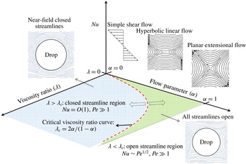
), there are two fundamentally distinct regimes of heat transport (see figure 1). This must accordingly reflect in the differing scaling of
 $Nu$
when plotted as a function of
 $\unicode[STIX]{x1D6FC}$
and
 $\unicode[STIX]{x1D706}$
for large
 $Pe$
; further, the character of this scaling may remain unchanged for sufficiently small drop deformation.
Schematic of the open- and closed-streamline regimes separated by the critical viscosity ratio curve
 $\unicode[STIX]{x1D706}_{c}(\unicode[STIX]{x1D6FC})=2\unicode[STIX]{x1D6FC}/(1-\unicode[STIX]{x1D6FC})$
(red dashed curve). The open-streamline regime (green hatched region) occurs for
 $\unicode[STIX]{x1D706}<\unicode[STIX]{x1D706}_{c}(\unicode[STIX]{x1D6FC})$
and is characterized by a boundary-layer-enhanced transfer with
 $Nu\propto Pe^{1/2}$
; inertia does not affect the transport at leading order.

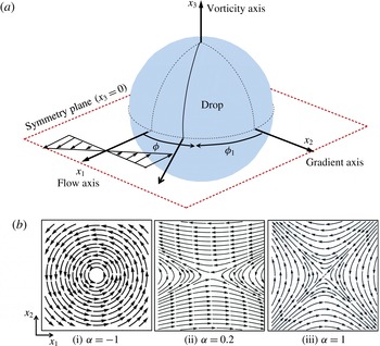
(a) Schematic of the coordinate system used showing the flow, gradient and vorticity axes for the particular case of an ambient simple shear flow. (b) Planar linear flows form a one-parameter family, the parameter
 $\unicode[STIX]{x1D6FC}$
ranging from
 $-1$
to
 $1$
. Canonical members of this family include (i) solid-body rotation (
 $\unicode[STIX]{x1D6FC}=-1$
), simple shear (
 $\unicode[STIX]{x1D6FC}=0$
) and (iii) planar extension (
 $\unicode[STIX]{x1D6FC}=1$
). The elliptic linear flows with
 $-1\leqslant \unicode[STIX]{x1D6FC}<0$
have closed streamlines, while the hyperbolic linear flows (ii) with
 $0<\unicode[STIX]{x1D6FC}\leqslant 1$
have open streamlines extending to infinity.

The problem of transport from an immiscible drop at high
 $Pe$
, and with
 $Re=0$
, remains unsolved for a general linear flow, and an expression for
 $Nu$
, along the lines of that obtained by Batchelor (Reference Batchelor1979) for a solid particle, is not available. The rate of transport, for large
 $Pe$
, has been obtained for relatively simple ambient flows including uniform flow (Leal Reference Leal2007), an axisymmetric extensional flow (Gupalo & Riazantsev Reference Gupalo and Riazantsev1972) and a combination of the two (Gupalo, Riazantsev & Ulin Reference Gupalo, Riazantsev and Ulin1975). The flow field in all cases is axisymmetric, the surface streamlines being meridians in a spherical coordinate system with its polar axis aligned with the symmetry axis of the flow, and the boundary-layer analysis therefore remains similar to those given as textbook examples (see Leal (Reference Leal2007)). The only other analysis is by Polyanin (Reference Polyanin1984) for a neutrally buoyant drop in a planar extensional flow. This again conforms to the open streamline regime, allowing for the approach used by Batchelor (Reference Batchelor1979) involving a boundary-layer analysis in an orthogonal streamline-aligned coordinate system (for a particle, the constant-coordinate lines on the surface are tangential to the local stress vector; these so-called von Mises coordinates have been used in traditional momentum boundary-layer analyses; see Schlichting & Gersten (Reference Schlichting and Gersten2001)). The large-
 $Pe$
scaling for
 $Nu$
, in the open-streamline regime, may be estimated in a manner similar to the particle. The boundary layer thickness
 $\unicode[STIX]{x1D6FF}$
is set by a balance of the convective time scale of
 $O(\dot{\unicode[STIX]{x1D6FE}}^{-1})$
and the diffusion time scale of
 $O(\unicode[STIX]{x1D6FF}^{2}/D)$
, giving
 $\unicode[STIX]{x1D6FF}\sim Pe^{-1/2}$
. This leads to
 $Nu\propto Pe^{1/2}$
. The rate of transport from a drop is asymptotically larger than that from a particle at the same
 $Pe$
, since the no-slip boundary condition in the latter case weakens the near-surface convection. The absence of closed-form expressions, for a general linear flow, for the prefactor (a function of the flow parameters) that multiplies
 $Pe^{1/2}$
in the above
 $Nu$
-scaling relation, stems from the complication introduced by the slip boundary condition. The no-slip boundary condition for particles makes the analysis significantly simpler. For particles in ambient linear flows with vorticity, for instance, the near-surface velocity field is dominated by the angular velocity of the rotating particle, the contribution due to the rate-of-strain tensor being asymptotically small. This allows for an averaging with respect to the azimuth in a spherical coordinate system with its polar axis along the angular velocity vector, an approach used by Batchelor (Reference Batchelor1979, Reference Batchelor1980); the azimuthally averaged convection–diffusion equation is similar to the aforementioned simpler axisymmetric flows, in that the azimuthally averaged convection is in the meridional direction. Physically, in linear flows with vorticity, the streamlines in the boundary layer are tightly wound spirals, and the azimuthal averaging isolates the convection that occurs across the spiral turns, and is responsible for carrying away heat or mass. For drops, the surface velocity field has comparable contributions from both the rate-of-strain and vortical components, and there is no obvious symmetry for an analysis to exploit for a general linear flow. Further, as already mentioned above, a second complication arises for the specific case of planar linear flows, in that the drop is surrounded by a region of closed streamlines in certain regions of the
 $(\unicode[STIX]{x1D6FC},\unicode[STIX]{x1D706})$
plane. In these cases, even weak departures from the Stokesian scenario, due to inertia or viscoelasticity (or other sources of microscopic irreversibility), is expected to have a major effect on the otherwise diffusion-limited transport rate. The singular effects of inertia and viscoelasticity have been studied for particles (Subramanian & Koch Reference Subramanian and Koch2006a
,Reference Subramanian and Koch
b
, Reference Subramanian and Koch2007), but not for drops.
In this paper, we restrict ourselves to analysing the convectively enhanced transport from a drop for two classes of ambient flows (i) planar linear flows in the with
 $\unicode[STIX]{x1D706}<\unicode[STIX]{x1D706}_{c}$
(which automatically excludes elliptic linear flows) and (ii) three-dimensional (linear) extensional flows, both of which conform to the open-streamline regime. In § 2, we present an analysis of the surface and near-field streamlines for a drop in a planar linear flow. After presenting the governing equation and boundary conditions for the dimensionless temperature field in § 3.1, § 3.2 is devoted to the large-
 $Pe$
boundary-layer analysis, where we solve the transport problem for a planar linear flow using a novel non-orthogonal coordinate system. This physically motivated coordinate system, derived in § 3.2.1, is based on the insight that the equations for the surface streamlines in this case can be reduced, under suitable transformations, to the Jeffery-orbit equations for an axisymmetric particle in a planar linear flow (Leal & Hinch Reference Leal and Hinch1971; Hinch & Leal Reference Hinch and Leal1972); the particle aspect ratio in the original instance maps to an
 $(\unicode[STIX]{x1D6FC},\unicode[STIX]{x1D706})$
-dependent effective aspect ratio in the present case. We use this coordinate system to find a similarity solution to the governing convection–diffusion equation in § 3.2.2, and derive an expression for the Nusselt number in § 3.2.3. The methodology remains valid for a general linear flow. To illustrate this, in § 3.3, we solve the transport problem for neutrally buoyant drops in the one-parameter family of linear extensional flows using a generalized version of the coordinate system used in § 3.2. The parameter here is
 $\unicode[STIX]{x1D716}$
, with
 $(1-\unicode[STIX]{x1D716})$
characterizing the departure of the extensional flow from axisymmetry; planar (
 $\unicode[STIX]{x1D716}=0$
) and axisymmetric (
 $\unicode[STIX]{x1D716}=1$
) extension are limiting members of this family. The Nusselt number is obtained in § 3.3. For both classes of flows,
 $Nu\propto Pe^{1/2}$
, with the boundary-layer analysis yielding closed-form expressions for the prefactor that is a function of
 $\unicode[STIX]{x1D6FC}$
and
 $\unicode[STIX]{x1D706}$
for planar linear flows, and a function of
 $\unicode[STIX]{x1D716}$
and
 $\unicode[STIX]{x1D706}$
for extensional flows. As a validation of our method, we show in § 3.3.4 that for the two special cases of planar (
 $\unicode[STIX]{x1D6FC}=1$
or
 $\unicode[STIX]{x1D716}=0$
) and axisymmetric extension, the Nusselt number predicted agrees exactly with earlier results given in Gupalo & Riazantsev (Reference Gupalo and Riazantsev1972) and Polyanin (Reference Polyanin1984), and obtained using a boundary-layer analysis in an orthogonal coordinate system; in appendix B, we also rederive Batchelor’s original result (Batchelor Reference Batchelor1979) for the large-
 $Pe$
transport from a particle in an extensional flow, using the analogue of the aforementioned non-orthogonal surface-streamline coordinates for a no-slip surface. In § 4 we present a summary of the work, and a detailed discussion on how, for a general linear flow, the present analysis may be extended to account for a finite transport resistance in the interior phase. Lagrangian chaos plays a crucial in these arguments. In a companion paper (Krishnamurthy & Subramanian Reference Krishnamurthy and Subramanian2018), we examine the transport from drops in planar linear flows that correspond to the closed-streamline regime (
 $\unicode[STIX]{x1D706}>\unicode[STIX]{x1D706}_{c}$
) in the
 $(\unicode[STIX]{x1D6FC},\unicode[STIX]{x1D706})$
plane. In this regime, weak inertial effects lead to convective enhancements at large
 $Pe$
, with the inertially enhanced heat transfer rate expected to scale as
 $Nu\propto O(RePe)^{1/2}$
. The non-orthogonal coordinate system based methodology developed here is used to derive the closed-form expression for the
 $(\unicode[STIX]{x1D6FC},\unicode[STIX]{x1D706})$
-dependent prefactor in the above scaling relation, that then quantitatively characterizes the inertially enhanced rate of transport.
2 Spherical drop in a planar linear flow: the Stokesian flow topology
Herein, we study the flow fields around and within a neutrally buoyant spherical drop immersed in an ambient Newtonian medium undergoing a planar linear flow. As already mentioned in § 1, these comprise a one-parameter family, the parameter
 $\unicode[STIX]{x1D6FC}$
being related to the ratio of vorticity to extension; the two-dimensionality implies that, the ambient vorticity vector is perpendicular to the plane of the ambient extension. Earlier efforts have studied the interior and exterior flow fields for a drop in simple shear (Torza et al.
Reference Torza, Henry, Cox and Mason1971) and in a general planar linear flow (Powell Reference Powell1983). Our motivation for revisiting this problem is to present a unified analysis of the interior and exterior streamlines. This naturally leads to three distinct regimes for the Stokesian streamline topology. The exterior flow topology in particular shows two distinct regimes: the open and closed-streamline regimes, with the drop in the latter case surrounded by an envelope of closed streamlines. Later, we focus on the surface streamlines, and derive a novel flow-aligned non-orthogonal coordinate system in § 3.2.1 which provides an appropriate framework for the large-
 $Pe$
analysis of the transport in the open-streamline regime.
2.1 Governing equations and boundary conditions
The viscosities and densities of the fluids inside and outside the drop are
 $\hat{\unicode[STIX]{x1D707}}$
,
 $\unicode[STIX]{x1D707}$
,
 $\hat{\unicode[STIX]{x1D70C}}$
and
 $\unicode[STIX]{x1D70C}$
, with the variables with carets corresponding to the interior fluid. Neutral buoyancy implies that
 $\hat{\unicode[STIX]{x1D70C}}=\unicode[STIX]{x1D70C}$
. For
 $Re=0$
, the governing equations in dimensionless form for the flow inside and outside the drop are, respectively, given by:
 $$\begin{eqnarray}\displaystyle \left.\begin{array}{@{}c@{}}-\unicode[STIX]{x1D735}\hat{p}+\unicode[STIX]{x1D706}\unicode[STIX]{x1D6FB}^{2}\hat{\boldsymbol{u}}=0\\ \unicode[STIX]{x1D735}\boldsymbol{\cdot }\hat{\boldsymbol{u}}=0\\ \end{array}\right\}\quad \text{interior problem,}\left.\begin{array}{@{}c@{}}-\unicode[STIX]{x1D735}p+\unicode[STIX]{x1D6FB}^{2}\boldsymbol{u}=0\\ \unicode[STIX]{x1D735}\boldsymbol{\cdot }\boldsymbol{u}=0\end{array}\right\}\quad \text{exterior problem,} & & \displaystyle \nonumber\\ \displaystyle & & \displaystyle\end{eqnarray}$$
where
 $\hat{\boldsymbol{u}}$
and
 $\boldsymbol{u}$
are the velocity fields in the drop interior and exterior, respectively;
 $\hat{p}$
and
 $p$
are the associated pressure fields;
 $\unicode[STIX]{x1D706}=\hat{\unicode[STIX]{x1D707}}/\unicode[STIX]{x1D707}$
is the drop to ambient fluid viscosity ratio. These equations are non-dimensionalized using the undeformed drop radius
 $a$
as a characteristic length scale, the characteristic scale
 $\dot{\unicode[STIX]{x1D6FE}}$
for the ambient velocity gradient times
 $a$
for the velocity scale; and identical viscous scalings for the interior and exterior pressure fields,
 $p_{c}=\hat{p}_{c}=\unicode[STIX]{x1D707}\dot{\unicode[STIX]{x1D6FE}}$
.
The ambient flow considered is given by
 $\boldsymbol{u}^{\infty }=\unicode[STIX]{x1D71E}\boldsymbol{\cdot }\boldsymbol{x}$
with the transpose of the velocity gradient tensor,
 $\unicode[STIX]{x1D71E}$
, given in dimensionless form by:
 $$\begin{eqnarray}\unicode[STIX]{x1D71E}=\left[\begin{array}{@{}ccc@{}}0 & -2 & 0\\ -2\unicode[STIX]{x1D6FC} & 0 & 0\\ 0 & 0 & 0\end{array}\right]\end{eqnarray}$$
in terms of
 $\unicode[STIX]{x1D6FC}$
.
 $\unicode[STIX]{x1D71E}$
can be written in terms of its symmetric and anti-symmetric components as
 $\unicode[STIX]{x1D71E}=\unicode[STIX]{x1D640}+\unicode[STIX]{x1D734}$
, where
 $\unicode[STIX]{x1D640}$
and
 $\unicode[STIX]{x1D734}$
are the rate-of-strain and vorticity tensors. Thus,
 $\unicode[STIX]{x1D6FC}$
in (2.2) measures the relative strengths of extension and vorticity, and is given by
 $\unicode[STIX]{x1D6FC}=(E-\unicode[STIX]{x1D6FA})/(E+\unicode[STIX]{x1D6FA})$
, where
 $2E/(E+\unicode[STIX]{x1D6FA})$
and
 $2\unicode[STIX]{x1D6FA}/(E+\unicode[STIX]{x1D6FA})$
denote the normalized magnitudes of the rate of extension and vorticity, respectively. The streamline patterns for a few members of this family are shown in figure 2(b). Since the paper is concerned with the open-streamline regime, the subset of ambient flows of interest are the hyperbolic linear flows; simple shear, with
 $\unicode[STIX]{x1D6FC}=0$
, being a limiting case. The coordinate system used for the subsequent analysis is depicted in figure 2(a), with
 $x_{1}$
,
 $x_{2}$
and
 $x_{3}$
being the flow, gradient and vorticity axes, respectively, of simple shear. The invariant directions of the hyperbolic flows are inclined to these axes, but the aforementioned terminology will nevertheless be used for all ambient flows.
The boundary conditions to be imposed are given by:
 $$\begin{eqnarray}\left.\begin{array}{@{}c@{}}\boldsymbol{u}^{\prime }\rightarrow 0\quad \text{as }r\rightarrow \infty \quad \text{(disturbance velocity decays off at infinity)}\\ \hat{\boldsymbol{u}}=\boldsymbol{u}^{\prime }+\unicode[STIX]{x1D71E}\boldsymbol{\cdot }\boldsymbol{x}\quad \text{at }r=1\quad \text{(continuity of velocity at interface)}\\ \boldsymbol{u}\boldsymbol{\cdot }\hat{n}=\hat{\boldsymbol{u}}\boldsymbol{\cdot }\hat{\boldsymbol{n}}=0\quad r=1\quad \text{(stationary spherical interface),}\\ (\unicode[STIX]{x1D748}\boldsymbol{\cdot }\hat{\boldsymbol{n}})\boldsymbol{\cdot }(\boldsymbol{I}-\hat{\boldsymbol{n}}\hat{\boldsymbol{n}})=(\hat{\unicode[STIX]{x1D748}}\boldsymbol{\cdot }\hat{\boldsymbol{n}})\boldsymbol{\cdot }(\boldsymbol{I}-\hat{\boldsymbol{n}}\hat{\boldsymbol{n}})\quad \text{at }r=1\\ \text{(continuity of tangential stress at the interface)},\end{array}\right\}\end{eqnarray}$$
where
 $\boldsymbol{u}^{\prime }$
is the exterior disturbance velocity due to the drop,
 $\hat{\boldsymbol{n}}$
is the unit radial vector and
 $\unicode[STIX]{x1D748}$
,
 $\hat{\unicode[STIX]{x1D748}}$
are the stress tensors in the exterior and interior fluid, respectively. Note that the normal stress balance at
 $r=1$
is not required to solve the system of equations for the velocity and pressure fields due to the assumed spherical shape of the interface. This condition may be used a posteriori to calculate the
 $O(Ca)$
drop deformation.
The solution of (2.1) subject to the above boundary conditions is well known (Cox Reference Cox1969; Leal Reference Leal2007). In spherical polar coordinates, with the polar axis aligned along the ambient vorticity, the components of the velocity field are given by:
 $$\begin{eqnarray}\displaystyle & \displaystyle u_{r}=-(1+\unicode[STIX]{x1D6FC})r[A(r;\unicode[STIX]{x1D706})r^{2}+B(r;\unicode[STIX]{x1D706})]\sin ^{2}\unicode[STIX]{x1D703}\sin 2\unicode[STIX]{x1D719}, & \displaystyle\end{eqnarray}$$
 $$\begin{eqnarray}\displaystyle & \displaystyle u_{\unicode[STIX]{x1D703}}=-{\displaystyle \frac{(1+\unicode[STIX]{x1D6FC})}{2}}rB(r;\unicode[STIX]{x1D706})\sin 2\unicode[STIX]{x1D703}\sin 2\unicode[STIX]{x1D719}, & \displaystyle\end{eqnarray}$$
 $$\begin{eqnarray}\displaystyle & \displaystyle u_{\unicode[STIX]{x1D719}}=-(1+\unicode[STIX]{x1D6FC})r\sin \unicode[STIX]{x1D703}[B(r;\unicode[STIX]{x1D706})\cos 2\unicode[STIX]{x1D719}-\unicode[STIX]{x1D6FD}], & \displaystyle\end{eqnarray}$$
where
 $\unicode[STIX]{x1D6FD}=(1-\unicode[STIX]{x1D6FC})/(1+\unicode[STIX]{x1D6FC})$
.
 $A(r;\unicode[STIX]{x1D706})$
and
 $B(r;\unicode[STIX]{x1D706})$
are functions of
 $r$
and
 $\unicode[STIX]{x1D706}$
which take different forms in the interior and exterior, being given by:
 $$\begin{eqnarray}\displaystyle & \displaystyle \left.\begin{array}{@{}c@{}}A(\unicode[STIX]{x1D706})=-{\displaystyle \frac{1}{1+\unicode[STIX]{x1D706}}},\\ B(r;\unicode[STIX]{x1D706})={\displaystyle \frac{5r^{2}-3}{2(1+\unicode[STIX]{x1D706})}}\\ \end{array}\right\}\quad \text{interior} & \displaystyle\end{eqnarray}$$
 $$\begin{eqnarray}\displaystyle & \displaystyle \left.\begin{array}{@{}c@{}}A(r;\unicode[STIX]{x1D706})=-{\displaystyle \frac{5\unicode[STIX]{x1D706}+2}{2(\unicode[STIX]{x1D706}+1)r^{5}}}+{\displaystyle \frac{5\unicode[STIX]{x1D706}}{2(1+\unicode[STIX]{x1D706})r^{7}}},\\ B(r;\unicode[STIX]{x1D706})=1-{\displaystyle \frac{\unicode[STIX]{x1D706}}{(1+\unicode[STIX]{x1D706})r^{5}}}.\end{array}\right\}\quad \text{exterior} & \displaystyle\end{eqnarray}$$
2.2 Analysis of interior and exterior streamlines
The Stokes streamlines corresponding to (2.4)–(2.6) may be regarded as the curves of intersection of invariant streamsurfaces (an approach first used in the context of rigid particles by Cox et al. (Reference Cox, Zia and Mason1968)), and are defined by Batchelor (Reference Batchelor2000):
 $$\begin{eqnarray}{\displaystyle \frac{\text{d}r}{u_{r}}}={\displaystyle \frac{r\,\text{d}\unicode[STIX]{x1D703}}{u_{\unicode[STIX]{x1D703}}}}={\displaystyle \frac{r\sin \unicode[STIX]{x1D703}\,\text{d}\unicode[STIX]{x1D719}}{u_{\unicode[STIX]{x1D719}}}}.\end{eqnarray}$$
Integrating the relations between velocities in the
 $r$
and
 $\unicode[STIX]{x1D703}$
directions, and
 $\unicode[STIX]{x1D703}$
and
 $\unicode[STIX]{x1D719}$
directions, one obtains the equations for the streamsurfaces characterizing the interior flow as:
 $$\begin{eqnarray}\displaystyle & \displaystyle x_{2}=\pm r\left[{\displaystyle \frac{1}{2}}-{\displaystyle \frac{\unicode[STIX]{x1D6FD}(1+\unicode[STIX]{x1D706})}{2r^{2}}}+\hat{E}r^{-2}(1-r^{2})^{-2/3}\right]^{1/2}, & \displaystyle\end{eqnarray}$$
 $$\begin{eqnarray}\displaystyle & \displaystyle x_{3}=\hat{D}(1-r^{2})^{-1/3}, & \displaystyle\end{eqnarray}$$
where
 $\hat{D}$
and
 $\hat{E}$
identify the streamsurfaces which intersect in a streamline, thus serving as interior streamline labels. Note from (2.10) and (2.11) that the constant-
 $\hat{D}$
and
 $\hat{E}$
surfaces are surfaces of revolution about the
 $x_{3}$
and
 $x_{2}$
axes, respectively (figure 3). Similarly, the exterior streamsurfaces are given by:
 $$\begin{eqnarray}\displaystyle & \displaystyle x_{2}=\pm r\left[{\displaystyle \frac{\unicode[STIX]{x1D6FC}}{(1+\unicode[STIX]{x1D6FC})}}+Ef(r)^{2}+{\displaystyle \frac{\unicode[STIX]{x1D6FD}\unicode[STIX]{x1D706}}{(1+\unicode[STIX]{x1D706})}}f(r)^{2}g(r)\right]^{1/2}, & \displaystyle\end{eqnarray}$$
 $$\begin{eqnarray}\displaystyle & \displaystyle x_{3}=rDf(r), & \displaystyle\end{eqnarray}$$
where
 $D$
and
 $E$
are the exterior streamsurfaces labels. Here,
 $f(r)=[r^{3}-(5\unicode[STIX]{x1D706}+2)/(2(\unicode[STIX]{x1D706}+1))+3\unicode[STIX]{x1D706}/(2(\unicode[STIX]{x1D706}+1))r^{-2}]^{-1/3}$
and
 $g(r)=\int _{r}^{\infty }f(y)y^{-3}\text{d}y$
. Just as in the interior case, the constant-
 $D$
and
 $E$
surfaces are surfaces of revolution about the
 $x_{3}$
and
 $x_{2}$
axes. The projections of these streamsurface families on the
 $(x_{1},x_{2})$
and
 $(x_{2},x_{3})$
planes are depicted in figure 3. As evident from the figure, the spherical drop, with
 $D=\hat{D}=E=\hat{E}=0$
is a limiting member of both families. For the constant-
 $D$
(or
 $\hat{D}$
) surfaces, this singular surface includes the drop and the intersecting plane of symmetry. For the constant-
 $E$
(or
 $\hat{E}$
) case, the singular surface can assume one of two forms: for
 $\unicode[STIX]{x1D706}<\unicode[STIX]{x1D706}_{c}$
(
 $\unicode[STIX]{x1D706}_{c}$
is given later in the section), the limiting surface includes both the drop and the intersecting separatrix surfaces that divide the exterior streamlines into open and recirculating ones (this is the case shown in figure 3
b); for
 $\unicode[STIX]{x1D706}>\unicode[STIX]{x1D706}_{c}$
, the spherical drop alone is the limiting surface.
To begin with, consider the streamlines lying in the equatorial plane (
 $x_{3}=0$
; the plane of symmetry) for which
 $D=\hat{D}=0$
. One may nevertheless extract features outside this plane by virtue of the axial symmetry properties of the constant-
 $E$
and
 $\hat{E}$
surfaces. These surfaces are given by (2.10) and (2.12), and subject to the constraint that
 $0\leqslant |x_{2}|\leqslant r$
, which results in the following inequalities to be satisfied by the interior streamlines (Powell Reference Powell1983):
 $$\begin{eqnarray}\displaystyle & \displaystyle \hat{E}\leqslant {\displaystyle \frac{(1-r^{2})^{2/3}}{2}}[\unicode[STIX]{x1D6FD}(1+\unicode[STIX]{x1D706})+r^{2}]=\hat{F}_{1}(r;\unicode[STIX]{x1D6FC},\unicode[STIX]{x1D706}), & \displaystyle\end{eqnarray}$$
 $$\begin{eqnarray}\displaystyle & \displaystyle \hat{E}\geqslant {\displaystyle \frac{(1-r^{2})^{2/3}}{2}}[\unicode[STIX]{x1D6FD}(1+\unicode[STIX]{x1D706})-r^{2}]=\hat{F}_{2}(r;\unicode[STIX]{x1D6FC},\unicode[STIX]{x1D706}). & \displaystyle\end{eqnarray}$$
The exterior streamlines, on the other hand, must satisfy:
 $$\begin{eqnarray}\displaystyle & \displaystyle E\leqslant {\displaystyle \frac{1}{(1+\unicode[STIX]{x1D6FC})f(r)^{2}}}-{\displaystyle \frac{\unicode[STIX]{x1D6FD}\unicode[STIX]{x1D706}g(r)}{1+\unicode[STIX]{x1D706}}}=F_{1}(r;\unicode[STIX]{x1D6FC},\unicode[STIX]{x1D706}), & \displaystyle\end{eqnarray}$$
 $$\begin{eqnarray}\displaystyle & \displaystyle E\geqslant {\displaystyle \frac{-\unicode[STIX]{x1D6FC}}{(1+\unicode[STIX]{x1D6FC})f(r)^{2}}}-{\displaystyle \frac{\unicode[STIX]{x1D6FD}\unicode[STIX]{x1D706}g(r)}{1+\unicode[STIX]{x1D706}}}=F_{2}(r;\unicode[STIX]{x1D6FC},\unicode[STIX]{x1D706}). & \displaystyle\end{eqnarray}$$
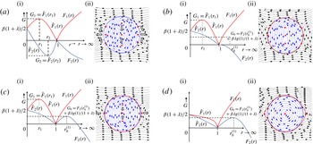
The spatial extent and nature of the streamlines can now be understood based on the behaviour of the functions
 $\hat{F}_{1}(r)$
,
 $\hat{F}_{2}(r)$
,
 $F_{1}(r)$
and
 $F_{2}(r)$
given in (2.14)–(2.17). For a given streamline (identified by the pair of streamline labels,
 $(D,E)$
or
 $(\hat{D},\hat{E})$
), one may calculate the interval in the radial coordinate, (
 $r_{min}$
,
 $r_{max}$
), for which the above relationships are satisfied. When the lower and upper bounds for the radial coordinate of a streamline are both finite, the streamline must be closed. Open streamlines, on the other hand, are characterized by an interval in the radial coordinate where the upper bound is infinity and the lower bound corresponds to the distance of closest approach.
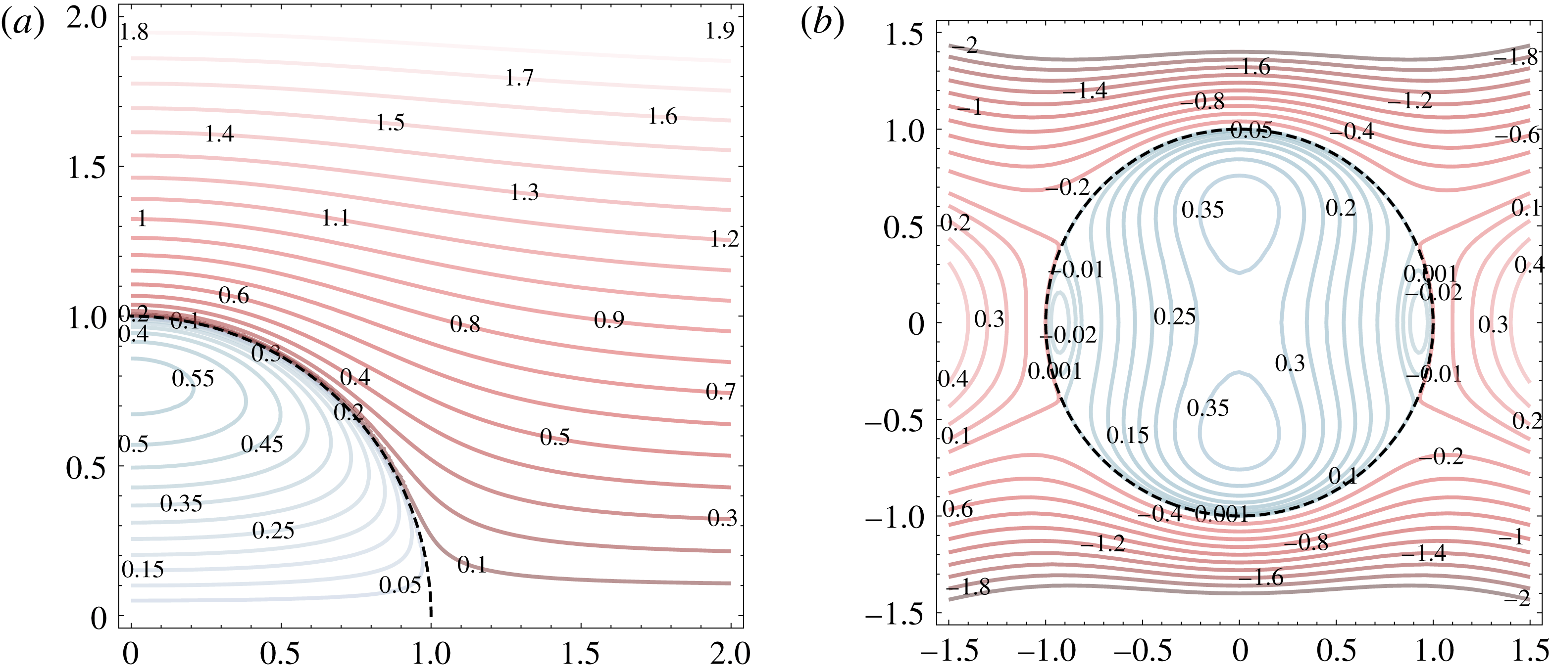
Interior and exterior streamsurfaces for a drop in a planar linear flow (
 $\unicode[STIX]{x1D6FC}=0.5$
and
 $\unicode[STIX]{x1D706}=1$
). (a) Projections of
 $\text{constant-}\hat{D}$
(blue) and
 $D$
(red) streamsurfaces in the
 $(x_{1},x_{3})$
plane; they are surfaces of revolution about the
 $x_{3}$
axis. The drop surface (dashed line), together with the symmetry plane (
 $x_{3}=0$
), make up the singular surface with
 $\hat{D}=D=0$
. (b) Projections of the
 $\text{constant-}\hat{E}$
(blue) and
 $E$
(red) surfaces in the
 $(x_{1},x_{2})$
plane; these are surfaces of revolution about the
 $x_{2}$
axis. The drop surface along with the separatrices is again a limiting singular surface with
 $\hat{E}=E=0$
. The streamsurface labels correspond to the values of
 $D,\hat{D}$
and
 $E,\hat{E}$
in (a) and (b), respectively.

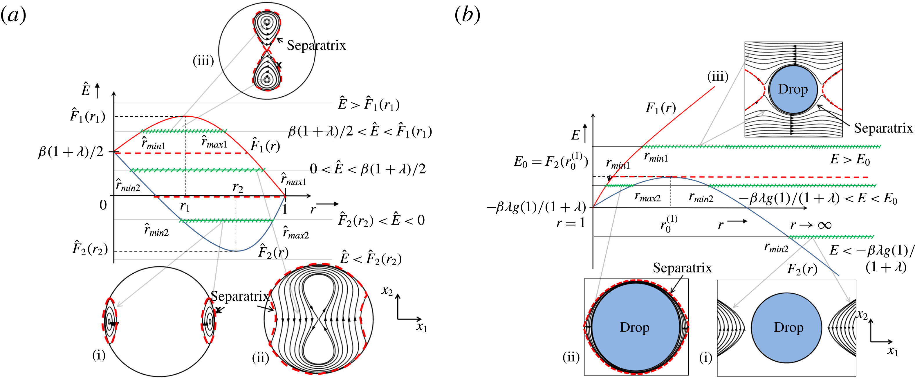
Plots of (a)
 $\hat{F}_{1}(r)$
and
 $\hat{F}_{2}(r)$
with respect to
 $r$
in the interior region. (b) Plots of
 $F_{1}(r)$
and
 $F_{2}(r)$
with respect to
 $r$
in the exterior region. Horizontal lines denote different values of the streamline label
 $\hat{E}$
and
 $E$
. There are three classes of interior and exterior streamlines (in general) which are labelled (i), (ii) and (iii). The green dashes depict the allowed range in
 $r$
of a given class of streamlines. Black arrows connect each of the green hashed lines to the corresponding class of streamlines. Red (dashed) arrows connect the red dashed lines to the separatrix streamlines which separate two different classes of streamlines.

The general qualitative behaviour of the interior and exterior bounding functions is sketched in figures 4(a) and 4(b), respectively. In the figures, a streamline is depicted as a horizontal hatched line with its endpoints, the radial coordinates of nearest and farthest approach, on one of the bounding curves identified above (
 $F_{i}(r)$
or
 $\hat{F}_{i}(r)$
) or at infinity. From figure 4(a), the interior bounding function
 $\hat{F}_{1}(r)$
is seen to vary in a non-monotonic manner from
 $\unicode[STIX]{x1D6FD}(1+\unicode[STIX]{x1D706})/2$
at
 $r=0$
to zero at
 $r=1$
with a single maximum at
 $\hat{r}_{0}^{1}=[3/5-(2/5)\unicode[STIX]{x1D6FD}(1+\unicode[STIX]{x1D706})]^{1/2}$
. From (2.4)–(2.6), and owing to the axial symmetry of the constant-
 $\hat{E}$
surfaces, the radial location of this maximum is a circle of fixed- points (fixed circle) of the interior flow, lying in the
 $(x_{2},x_{3})$
plane and given by
 $\{{\hat{r}_{0}}^{1},{\hat{\unicode[STIX]{x1D703}}_{0}}^{1},{\hat{\unicode[STIX]{x1D719}}_{0}}^{1}\}=\{[3/5-(2/5)\unicode[STIX]{x1D6FD}(1+\unicode[STIX]{x1D706})]^{1/2},\unicode[STIX]{x1D703},(\unicode[STIX]{x03C0}/2,3\unicode[STIX]{x03C0}/2)\}$
(see figure 5
aii). Similarly,
 $\hat{F}_{2}(r)$
varies between the same two limits as
 $\hat{F}_{1}(r)$
, but with an intermediate minimum at
 $\hat{r}_{0}^{2}=[3/5+(2/5)\unicode[STIX]{x1D6FD}(1+\unicode[STIX]{x1D706})]^{1/2}$
(see figure 4
a). The radial location of this minimum corresponds to a second fixed circle of the interior flow, lying in the
 $(x_{1},x_{3})$
plane and given by
 $\{{\hat{r}_{0}}^{2},{\hat{\unicode[STIX]{x1D703}}_{0}}^{2},{\hat{\unicode[STIX]{x1D719}}_{0}}^{2}\}=\{[3/5+(2/5)\unicode[STIX]{x1D6FD}(1+\unicode[STIX]{x1D706})]^{1/2},\unicode[STIX]{x1D703},(0,\unicode[STIX]{x03C0})\}$
(figure 5
a). It is straightforward to see that
 $\hat{r}_{0}^{2}\geqslant \hat{r}_{0}^{1}$
and that equality occurs only when
 $\unicode[STIX]{x1D6FD}=0$
(
 $\unicode[STIX]{x1D6FC}=1$
; planar extension, as must be the case by symmetry) for any
 $\unicode[STIX]{x1D706}$
. Additionally, we find two other pairs of fixed points that lie on the drop surface in the equatorial plane (
 $x_{3}=0$
), which correspond to the intersection of the two bounding curves at
 $\hat{E}=0$
. One member of each pair is given by
 $\{{\hat{r}_{0}}^{3},{\hat{\unicode[STIX]{x1D703}}_{0}}^{3},{\hat{\unicode[STIX]{x1D719}}_{0}}^{3}\}=\{1,\unicode[STIX]{x03C0}/2,\cos ^{-1}[\unicode[STIX]{x1D6FD}(1+\unicode[STIX]{x1D706})]/2\}$
and
 $\{{\hat{r}_{0}}^{4},{\hat{\unicode[STIX]{x1D703}}_{0}}^{4},{\hat{\unicode[STIX]{x1D719}}_{0}}^{4}\}=\{1,\unicode[STIX]{x03C0}/2,-\cos ^{-1}[\unicode[STIX]{x1D6FD}(1+\unicode[STIX]{x1D706})]/2\}$
. By symmetry, the other member is at a
 $\unicode[STIX]{x03C0}$
-separated location in
 $\unicode[STIX]{x1D719}$
.
Depiction of the three regimes of the interior and exterior flow field for a drop in an ambient planar linear flow (
 $\unicode[STIX]{x1D6FC}=0.25$
). (a)
 $0\leqslant \unicode[STIX]{x1D706}\leqslant \unicode[STIX]{x1D706}_{c}(\unicode[STIX]{x1D6FC})$
, (b)
 $\unicode[STIX]{x1D706}=\unicode[STIX]{x1D706}_{c}$
(c)
 $\unicode[STIX]{x1D706}_{c}(\unicode[STIX]{x1D6FC})<\unicode[STIX]{x1D706}\leqslant \unicode[STIX]{x1D706}_{c}^{\prime }(\unicode[STIX]{x1D6FC})$
and (d)
 $\unicode[STIX]{x1D706}_{c}^{\prime }(\unicode[STIX]{x1D6FC})<\unicode[STIX]{x1D706}<\infty$
. Part (i) of each figure depicts (schematically) the functions
 $\hat{F}_{1}(r)$
,
 $\hat{F}_{2}(r)$
,
 $F_{1}(r)$
and
 $F_{2}(r)$
and part (ii) of each figure is a plot of the streamlines (drop interior streamlines in blue and exterior streamlines in black) in the equatorial plane (
 $x_{3}=0$
). The red dots depict the fixed points in the flow, some of which are actually part of fixed circles (extending out of the plane), as described in the text. The hollow black arrows in (a) and (c) depict the direction of movement of the fixed points with increasing
 $\unicode[STIX]{x1D706}$
. The red dashed curves in (c) and (d) denote the extent of the closed-streamline region surrounding the drop.

The exterior bounding function
 $F_{1}(r)$
is a strictly increasing function with a minimum value of
 $-\unicode[STIX]{x1D6FD}\unicode[STIX]{x1D706}g(1)/(1+\unicode[STIX]{x1D706})$
at
 $r=1$
(figure 4
b).
 $F_{2}(r)$
has the same value at
 $r=1$
as
 $F_{1}(r)$
, and is non-monotonic with a single maximum at
 $r_{0}^{1}=[\unicode[STIX]{x1D706}(1+\unicode[STIX]{x1D6FC})/((1+\unicode[STIX]{x1D706})2\unicode[STIX]{x1D6FC})]^{1/5}$
. One can deduce from (2.4)–(2.6), and owing to the symmetry of the constant-
 $E$
surfaces, that this radial location is a fixed circle of the exterior flow field, lying in the
 $(x_{1},x_{3})$
plane and given by
 $(r_{0}^{1},\unicode[STIX]{x1D703}_{0}^{1},\unicode[STIX]{x1D719}_{0}^{1})=\{[\unicode[STIX]{x1D706}(1+\unicode[STIX]{x1D6FC})/((1+\unicode[STIX]{x1D706})2\unicode[STIX]{x1D6FC})]^{1/5},\unicode[STIX]{x1D703},(0,\unicode[STIX]{x03C0})\}$
. Note that the vorticity (
 $x_{3}$
axis) is a line of fixed points for both the drop interior and exterior for all
 $\unicode[STIX]{x1D6FC}$
and
 $\unicode[STIX]{x1D706}$
.
2.2.1 Combined analysis
The interior and exterior bounding functions are not independent of each other. For instance, for a given
 $(\unicode[STIX]{x1D6FC},\unicode[STIX]{x1D706})$
,
 $\hat{F}_{2}(r)$
cannot have a minimum in
 $r\in [0,1]$
, while
 $F_{2}(r)$
has a maximum in
 $r\in (1,\infty )$
. In other words, there is a transition between monotonicity and non-monotonicity (in opposite senses) for
 $\hat{F}_{2}(r)$
and
 $F_{2}(r)$
at the same critical value of
 $\unicode[STIX]{x1D706}$
. With regard to the earlier discussion, this implies that there is, in fact, only one fixed circle in the
 $(x_{1},x_{3})$
plane, of radius
 $[3/5+(2/5)\unicode[STIX]{x1D6FD}(1+\unicode[STIX]{x1D706})]^{1/2}$
, that appears either in the interior or exterior depending on the particular
 $\unicode[STIX]{x1D6FC}$
and
 $\unicode[STIX]{x1D706}$
; figure 4(a,b) therefore correspond to different
 $(\unicode[STIX]{x1D6FC},\unicode[STIX]{x1D706})$
pairs. An additional implication is that it must be possible to combine our analysis of the interior and exterior streamlines into one which is uniformly valid in the entire domain. To achieve this, one rewrites the streamline label
 $E$
in the exterior coordinate as
 $G=E+\unicode[STIX]{x1D6FD}\unicode[STIX]{x1D706}g(1)/(1+\unicode[STIX]{x1D706})$
, making the bounding functions continuous across the drop surface (
 $r=1$
). This allows
 $G$
to be the single streamline label for both the interior and exterior flows (
 $G=\hat{E}$
for
 $r<1$
and
 $G=E+\unicode[STIX]{x1D6FD}\unicode[STIX]{x1D706}g(1)/(1+\unicode[STIX]{x1D706})$
for
 $r>1$
).
Based on the behaviour of the combined (upper and lower) bounding functions, one finds two critical
 $\unicode[STIX]{x1D6FC}$
-dependent viscosity ratios
 $\unicode[STIX]{x1D706}_{c}(\unicode[STIX]{x1D6FC})$
and
 $\unicode[STIX]{x1D706}_{c}^{\prime }(\unicode[STIX]{x1D6FC})$
, in turn leading to three distinct regimes for the streamline topologies in the drop interior and exterior.
 $\unicode[STIX]{x1D706}_{c}(\unicode[STIX]{x1D6FC})$
is the value at which the minimum of
 $\hat{F}_{2}(r)$
and the maximum of
 $F_{2}(r)$
coincide at
 $r=1$
(figure 5
b). Thus,
 $\unicode[STIX]{x1D706}_{c}$
can be calculated by setting
 $r_{0}^{1}=\hat{r}_{0}^{2}=1$
, yielding:
 $$\begin{eqnarray}\unicode[STIX]{x1D706}_{c}(\unicode[STIX]{x1D6FC})=2\unicode[STIX]{x1D6FC}/(1-\unicode[STIX]{x1D6FC}).\end{eqnarray}$$
For
 $\unicode[STIX]{x1D706}<\unicode[STIX]{x1D706}_{c}$
, as mentioned earlier,
 $\hat{F}_{2}(r)$
has a minimum in
 $r\in [0,1]$
, while
 $F_{2}(r)$
is monotonically decreasing in
 $r\in [1,\infty )$
(figure 5
ai), while for
 $\unicode[STIX]{x1D706}_{c}<\unicode[STIX]{x1D706}<\unicode[STIX]{x1D706}_{c}^{\prime }$
,
 $\hat{F}_{2}(r)$
is monotonically decreasing while
 $F_{2}(r)$
has a maximum for
 $r\in [\!1,\infty \!)$
(figure 5
c). In a similar fashion, at
 $\unicode[STIX]{x1D706}=\unicode[STIX]{x1D706}_{c}^{\prime }$
, the maximum of
 $\hat{F}_{1}(r)$
lies at
 $r=0$
and for
 $\unicode[STIX]{x1D706}>\unicode[STIX]{x1D706}_{c}^{\prime }(\unicode[STIX]{x1D6FC})$
, the function
 $\hat{F}_{1}(r)$
is monotonically decreasing in
 $r\in [0,1]$
with a finite slope at
 $r=0$
(figure 5
di). This second critical viscosity ratio can therefore be calculated by solving
 ${\hat{r}_{0}}^{1}=0$
, giving:
 $$\begin{eqnarray}\unicode[STIX]{x1D706}_{c}^{\prime }=(5\unicode[STIX]{x1D6FC}+1)/(2(1-\unicode[STIX]{x1D6FC})).\end{eqnarray}$$
Let
 $G_{1}$
denote the maximum value of the function
 $\hat{F}_{1}(r)$
at
 $r_{1}$
,
 $G_{2}$
the minimum value of the function
 $\hat{F}_{2}(r)$
at
 $r_{2}$
, and
 $G_{0}$
the maximum value of the shifted function
 $F_{2}(r)+\unicode[STIX]{x1D6FD}\unicode[STIX]{x1D706}g(1)/(1+\unicode[STIX]{x1D706})$
attained at
 $r_{0}^{1}$
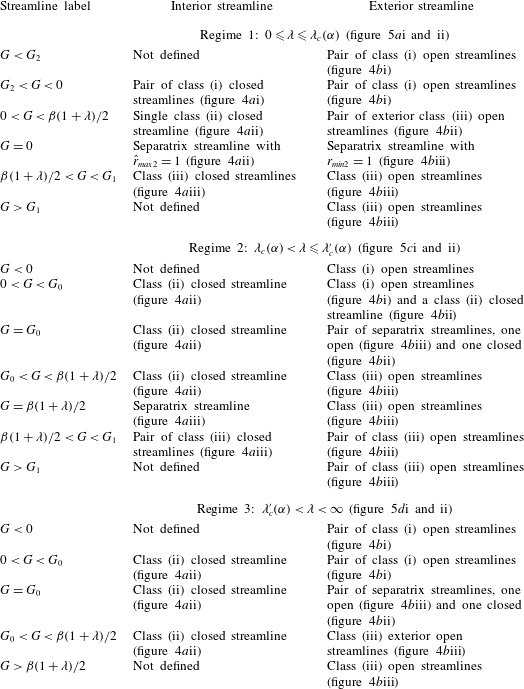
. In table 1, given in appendix A, the streamline topology for the three regimes (i)
 $0\leqslant \unicode[STIX]{x1D706}\leqslant \unicode[STIX]{x1D706}_{c}(\unicode[STIX]{x1D6FC})$
, (ii)
 $\unicode[STIX]{x1D706}_{c}(\unicode[STIX]{x1D6FC})<\unicode[STIX]{x1D706}\leqslant \unicode[STIX]{x1D706}_{c}^{\prime }(\unicode[STIX]{x1D6FC})$
and (iii)
 $\unicode[STIX]{x1D706}_{c}^{\prime }(\unicode[STIX]{x1D6FC})<\unicode[STIX]{x1D706}<\infty$
, based on the relative magnitudes of these extrema.
The transition in the streamline topology from one regime to the other, with increasing
 $\unicode[STIX]{x1D706}$
is shown in figure 5(a–d). For a fixed
 $\unicode[STIX]{x1D6FC}$
, as one increases
 $\unicode[STIX]{x1D706}$
from below
 $\unicode[STIX]{x1D706}_{c}$
, the first (and smaller) fixed circle in the drop interior at
 $\{{\hat{r}_{0}}^{1},{\hat{\unicode[STIX]{x1D703}}_{0}}^{1},{\hat{\unicode[STIX]{x1D719}}_{0}}^{1}\}$
decreases in radius, while the second (and larger) fixed circle at
 $\{{\hat{r}_{0}}^{2},{\hat{\unicode[STIX]{x1D703}}_{0}}^{2},{\hat{\unicode[STIX]{x1D719}}_{0}}^{2}\}$
increases in radius (see figure 5
a). At
 $\unicode[STIX]{x1D706}=\unicode[STIX]{x1D706}_{c}$
, this second fixed circle merges with the fixed points at
 $\{{\hat{r}_{0}}^{3},{\hat{\unicode[STIX]{x1D703}}_{0}}^{3},{\hat{\unicode[STIX]{x1D719}}_{0}}^{3}\}$
and
 $\{{\hat{r}_{0}}^{4},{\hat{\unicode[STIX]{x1D703}}_{0}}^{4},{\hat{\unicode[STIX]{x1D719}}_{0}}^{4}\}$
, which themselves move towards each other (along
 $r=1$
) for
 $\unicode[STIX]{x1D706}$
approaching
 $\unicode[STIX]{x1D706}_{c}$
, to form a fixed circle exactly on the drop surface (see figure 5
b). For
 $\unicode[STIX]{x1D706}>\unicode[STIX]{x1D706}_{c}$
, this fixed circle moves outside the drop and is now given by
 $\{r_{0}^{1},\unicode[STIX]{x1D703}_{0}^{1},\unicode[STIX]{x1D719}_{0}^{1}\}$
(see figure 5
c). Importantly, for
 $\unicode[STIX]{x1D706}>\unicode[STIX]{x1D706}_{c}$
there now exists an annular region of closed streamlines surrounding the drop whose maximum radial extent is given by
 $r_{0}^{1}$
(see figure 5
c,d). Thus,
 $\unicode[STIX]{x1D706}_{c}(\unicode[STIX]{x1D6FC})$
is the critical viscosity curve which separates the open- and closed-streamline regimes in the exterior field (see figure 1). These two regimes lead to fundamentally different mechanisms for the transport of heat or mass from drops at large
 $Pe$
. In the rest of the paper we solve the problem of transport from drops in the open-streamline regime where the effects of inertia do not affect the transport at leading order, except perhaps close to
 $\unicode[STIX]{x1D706}=\unicode[STIX]{x1D706}_{c}$
(see figure 1). As one increases
 $\unicode[STIX]{x1D706}$
further, the fixed circle in the drop interior continues to become smaller while the exterior fixed circle grows in size. At
 $\unicode[STIX]{x1D706}=\unicode[STIX]{x1D706}_{c}^{\prime }(\unicode[STIX]{x1D6FC})$
, the interior fixed circle shrinks to a point at the origin, leaving the origin as the only fixed point in the drop interior (although not relevant to the exterior transport problem analysed here, this transition in the interior streamline topology involving the disappearance of saddles for sufficiently high
 $\unicode[STIX]{x1D706}$
is likely to be important in chaotic advection leading to drop mixing (see Bryden & Brenner (Reference Bryden and Brenner1999))); the implications of chaos in the interior flow, for the transport rate at large
 $Pe$
, are further discussed in § 4. Note that the axisymmetric closed streamline region is infinite in volume for simple shear flow (
 $\unicode[STIX]{x1D6FC}=0$
) for any
 $\unicode[STIX]{x1D706}$
since the maximal extent of the region
 $r_{0}^{1}\rightarrow \infty$
for
 $\unicode[STIX]{x1D6FC}=0$
(with the ordinate decreasing as
 $r^{-3/2}$
, as a for a rigid sphere). For any
 $\unicode[STIX]{x1D6FC}\neq 0$
, this region grows in size for increasing
 $\unicode[STIX]{x1D706}$
, but asymptotes to a finite extent even as
 $\unicode[STIX]{x1D706}\rightarrow \infty$
.
3 Open-streamline transport from a drop
We now study the transport from a drop in the open-streamline regime corresponding to
 $\unicode[STIX]{x1D706}<\unicode[STIX]{x1D706}_{c}$
, when the drop surface is accessed by streamlines not confined to a finite domain. This ensures convectively enhanced transport to the ambient in the limit of large
 $Pe$
. Elementary scaling arguments in the introduction give
 $Nu\propto Pe^{1/2}$
, and the sections below calculate the prefactor in this relationship, that is a function of the flow-type parameter and
 $\unicode[STIX]{x1D706}$
, for different linear flows. Our approach utilizes a flow-aligned non-orthogonal coordinate system to arrive at an analytical solution. As is shown in appendix B, the approach also works for solid particles, and a portion of the original set of results of Batchelor (Reference Batchelor1979) is rederived therein using a different formulation in non-orthogonal coordinates.
3.1 Preliminaries and governing equations
Consider a drop whose surface is maintained at a constant temperature
 $T_{0}$
(amounting to the neglect of the interior phase resistance) suspended in an ambient fluid originally at
 $T_{\infty }$
. The presence of open streamlines near the drop surface implies that, for
 $Pe\gg 1$
almost the entire temperature drop occurs across a thin thermal boundary layer. The efficiency of transport is characterized by the Nusselt number, the ratio of the total heat transfer rate (
 $Q$
) to the transfer rate due to conduction alone, and given by
 $Nu=Q/[4\unicode[STIX]{x03C0}ka(T_{0}-T_{\infty })]$
,
 $k$
the thermal conductivity of the ambient fluid,
 $a$
is the drop radius (
 $Nu=1$
for purely conductive heat transfer).
Before moving on to the heat transfer problem for specific families of linear flows, it is instructive to examine the parametric dependence of
 $Nu$
for a drop in a general linear flow. An incompressible linear flow is characterized by a traceless velocity gradient tensor with eight independent pieces of information defining the flow. Factoring out the magnitude of the velocity gradient tensor (the shear rate) in
 $Pe$
, there are seven (dimensionless) pieces of information. For linear extensional flows, this reduces to only four since the velocity gradient tensor is symmetric, being identical to the rate-of-strain tensor. Three of these may be used in choosing a coordinate system aligned with the principal axes of the rate-of-strain tensor (
 $Nu$
being a scalar, cannot be dependent on this choice). The remaining piece measures the departure from axisymmetry of the rate-of-strain tensor. This parameter
 $\unicode[STIX]{x1D716}$
may be defined as the ratio of two principal rates of strain; thus,
 $\unicode[STIX]{x1D716}=E_{2}/E_{1}$
characterizes the second one-parameter family of flows considered here. For a general linear flow, three additional pieces of information remain. One of these measures the relative magnitudes of vorticity and extension. The remaining two fix the orientation of the vorticity vector relative to the principal axes. For planar linear flows, the first family considered in the analysis below, the vorticity vector is constrained to lie along the principal axis corresponding to the zero eigenvalue of the rate-of-strain tensor, leaving its (relative) magnitude, denoted by
 $\unicode[STIX]{x1D6FC}$
, as the only remaining parameter.
The heat transfer is governed by the convection–diffusion equation for the temperature field with the convection being driven by the Stokesian velocity field. For purposes of simplicity and to highlight the underlying physics, the heat transfer is assumed to be decoupled from the momentum conservation equations. Thus, changes in temperature are assumed not to lead to variations in the fluid properties. Neglect of temperature-induced density variations in particular makes this a forced convection problem (in dimensionless terms, this is equivalent to the Rayleigh number based on the drop size being negligible). The convection–diffusion equation in dimensionless form is (Leal Reference Leal2007)):
 $$\begin{eqnarray}Pe(\boldsymbol{u}.\unicode[STIX]{x1D735}\unicode[STIX]{x1D6E9})=\unicode[STIX]{x1D6FB}^{2}\unicode[STIX]{x1D6E9},\end{eqnarray}$$
where
 $\unicode[STIX]{x1D6E9}=(T-T_{\infty })/(T_{0}-T_{\infty })$
. The boundary conditions are given by:
 $$\begin{eqnarray}\displaystyle & \unicode[STIX]{x1D6E9}=1\quad \text{at }r=1\;(\text{Isothermal drop surface at }T_{0}), & \displaystyle\end{eqnarray}$$
 $$\begin{eqnarray}\displaystyle & \unicode[STIX]{x1D6E9}\rightarrow 0\quad \text{as }r\rightarrow \infty \;\text{(Ambient temperature at infinity)}. & \displaystyle\end{eqnarray}$$
The transport problem, in the stated form, is solved for two families of linear flows. In § 3.2, we consider the hyperbolic planar linear flows followed by three-dimensional extensional flows in § 3.3.
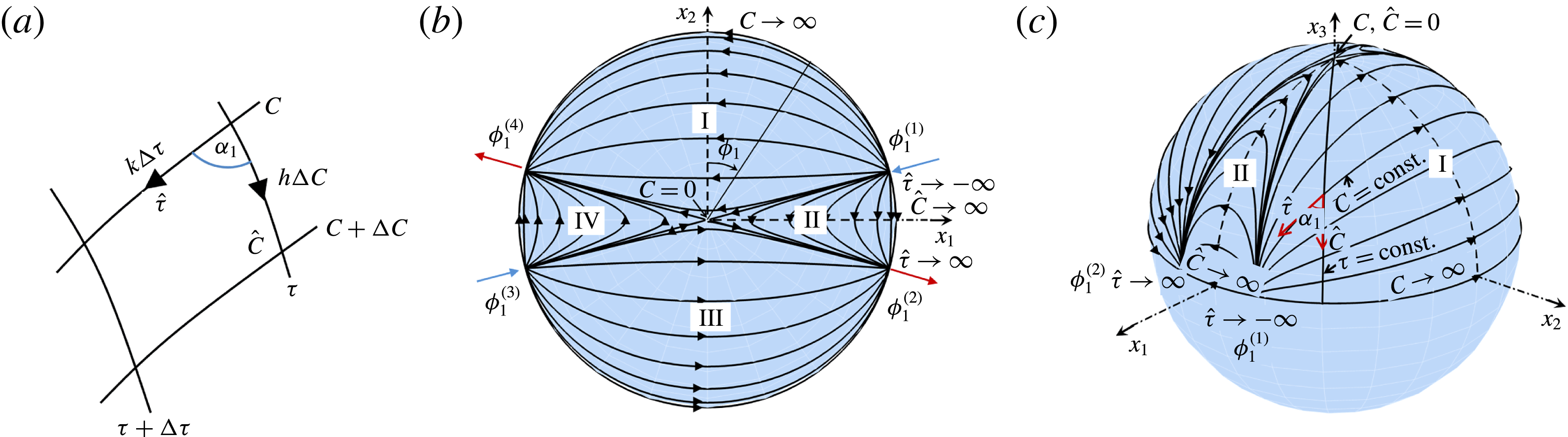
(a) The
 $(C,\unicode[STIX]{x1D70F})$
coordinate system and its metrics. The
 $(C,\unicode[STIX]{x1D70F})$
mapping on the drop surface in the open-streamline regime; surface streamlines projected onto the
 $(x_{1},x_{2})$
plane in (b) and presented in a three-dimensional view in (c). The four regions are marked I through IV, with regions (I, III) and (II, IV) being equivalent.
 $C$
and
 ${\hat{C}}$
act as surface-streamline labels in regions I and II, and vary from
 $0$
to
 $\infty$
at the equatorial plane. Except for
 $C={\hat{C}}=0$
, all streamlines begin and end at one of four equatorial-plane stagnation points;
 $\hat{\unicode[STIX]{x1D70F}}$
varies from
 $-\infty$
at the inlet to
 $+\infty$
at the outlet.

3.2 Drop in a planar linear flow
3.2.1 The
 $(C,\unicode[STIX]{x1D70F})$
coordinate system

We first analyse the streamlines on the drop surface, given that they determine the flow within the thermal boundary layer. Note that the ’open-streamline’ terminology refers to the nature of the exterior streamlines for
 $\unicode[STIX]{x1D706}<\unicode[STIX]{x1D706}_{c}$
. The surface streamlines in this regime cannot obviously be open. As will be seen, they begin and end at stagnation points of the surface tangential velocity field (figure 6
c). Since the drop is spherical and stationary, the radial velocity at the surface is identically zero, and the surface streamlines are determined by the velocity components in the
 $\unicode[STIX]{x1D703}$
and
 $\unicode[STIX]{x1D719}$
directions, obtained by setting
 $r=1$
in (2.5) and (2.6):
 $$\begin{eqnarray}\displaystyle & \displaystyle u_{\unicode[STIX]{x1D703}}|_{r=1}=-{\displaystyle \frac{(1+\unicode[STIX]{x1D6FC})}{2(1+\unicode[STIX]{x1D706})}}\sin 2\unicode[STIX]{x1D703}\sin 2\unicode[STIX]{x1D719}_{1}={\displaystyle \frac{\text{d}\unicode[STIX]{x1D703}}{\text{d}s}}, & \displaystyle\end{eqnarray}$$
 $$\begin{eqnarray}\displaystyle & \displaystyle u_{\unicode[STIX]{x1D719}}|_{r=1}={\displaystyle \frac{(1+\unicode[STIX]{x1D6FC})}{(1+\unicode[STIX]{x1D706})}}\sin \unicode[STIX]{x1D703}[\cos 2\unicode[STIX]{x1D719}_{1}+\unicode[STIX]{x1D6FD}(1+\unicode[STIX]{x1D706})]=-\sin \unicode[STIX]{x1D703}{\displaystyle \frac{\text{d}\unicode[STIX]{x1D719}_{1}}{\text{d}s}}, & \displaystyle\end{eqnarray}$$
where we have used the transformation
 $\unicode[STIX]{x1D719}_{1}=\unicode[STIX]{x03C0}/2-\unicode[STIX]{x1D719}$
, so that
 $\unicode[STIX]{x1D719}_{1}$
is measured from the
 $x_{2}$
axis (see figure 2
a). Also,
 $s$
is the dimensionless time (measured in units of
 $\dot{\unicode[STIX]{x1D6FE}}^{-1}$
) and
 $\unicode[STIX]{x1D6FD}=(1-\unicode[STIX]{x1D6FC})/(1+\unicode[STIX]{x1D6FC})$
. The above equations may be rewritten as:
 $$\begin{eqnarray}\displaystyle & \displaystyle {\displaystyle \frac{\text{d}\unicode[STIX]{x1D703}}{\text{d}s}}=-{\displaystyle \frac{(1-\unicode[STIX]{x1D6FC})(\unicode[STIX]{x1D6FE}^{2}-1)}{2(\unicode[STIX]{x1D6FE}^{2}+1)}}\sin 2\unicode[STIX]{x1D703}\sin 2\unicode[STIX]{x1D719}_{1}, & \displaystyle\end{eqnarray}$$
 $$\begin{eqnarray}\displaystyle & \displaystyle {\displaystyle \frac{\text{d}\unicode[STIX]{x1D719}_{1}}{\text{d}s}}=-{\displaystyle \frac{2(1-\unicode[STIX]{x1D6FC})}{\unicode[STIX]{x1D6FE}^{2}+1}}[\unicode[STIX]{x1D6FE}^{2}\cos ^{2}\unicode[STIX]{x1D719}_{1}+\sin ^{2}\unicode[STIX]{x1D719}_{1}], & \displaystyle\end{eqnarray}$$
where
 $$\begin{eqnarray}\unicode[STIX]{x1D6FE}=\left[{\displaystyle \frac{(\unicode[STIX]{x1D6FD}(1+\unicode[STIX]{x1D706})+1)}{(\unicode[STIX]{x1D6FD}(1+\unicode[STIX]{x1D706})-1)}}\right]^{1/2}=\left[{\displaystyle \frac{\unicode[STIX]{x1D706}_{c}+\unicode[STIX]{x1D6FC}~\unicode[STIX]{x1D706}}{\unicode[STIX]{x1D6FC}(\unicode[STIX]{x1D706}-\unicode[STIX]{x1D706}_{c})}}\right]^{1/2}.\end{eqnarray}$$
Comparing (3.6) and (3.7) to equations 2(a) and 2(b) in Leal & Hinch (Reference Leal and Hinch1971) (see also Hinch & Leal (Reference Hinch and Leal1972)), one notes that these have the exact same form as the equations for the Jeffery orbits of an axisymmetric particle in a planar linear flow. For the original Jeffery orbits in a simple shear flow (Leal & Hinch Reference Leal and Hinch1971),
 $\unicode[STIX]{x1D6FE}$
was a geometric quantity – being the true aspect ratio for spheroids, and an effective aspect ratio for other geometries (Trevelyan & Mason Reference Trevelyan and Mason1951; Cox Reference Cox1971). Generalization of the Jeffery orbits for planar linear flows results in an effective aspect ratio which is no longer a purely geometric quantity, being a function of both the actual aspect ratio and flow type (Hinch & Leal Reference Hinch and Leal1972; Marath & Subramanian Reference Marath and Subramanian2018). For the drop surface streamlines considered here there is no geometric quantity, and the effective aspect ratio is determined by the flow type (
 $\unicode[STIX]{x1D6FC}$
) and the viscosity ratio (
 $\unicode[STIX]{x1D706}$
).
The above insight allows one to define a new coordinate system to describe the surface streamlines. Proceeding as in Leal & Hinch (Reference Leal and Hinch1971), and integrating (3.7), one obtains:
 $$\begin{eqnarray}\tan \unicode[STIX]{x1D719}_{1}=\unicode[STIX]{x1D6FE}\tan {\displaystyle \frac{-2(1-\unicode[STIX]{x1D6FC})s}{\unicode[STIX]{x1D6FE}+1/\unicode[STIX]{x1D6FE}}}.\end{eqnarray}$$
Introducing a new variable
 $\unicode[STIX]{x1D70F}=(-2(1-\unicode[STIX]{x1D6FC})s)/(\unicode[STIX]{x1D6FE}+1/\unicode[STIX]{x1D6FE})$
, we have the equation:
 $$\begin{eqnarray}\tan \unicode[STIX]{x1D719}_{1}=\unicode[STIX]{x1D6FE}\tan \unicode[STIX]{x1D70F}.\end{eqnarray}$$
Similarly, we can integrate (3.6), after substituting for
 $\unicode[STIX]{x1D719}_{1}$
in terms of
 $\unicode[STIX]{x1D70F}$
, and one obtains:
 $$\begin{eqnarray}\tan \unicode[STIX]{x1D703}=C[\cos ^{2}\unicode[STIX]{x1D70F}+\unicode[STIX]{x1D6FE}^{2}\sin ^{2}\unicode[STIX]{x1D70F}]^{1/2}.\end{eqnarray}$$
The relations (3.10) and (3.11) form the basis of the
 $(C,\unicode[STIX]{x1D70F})$
coordinate system on the drop surface. As seen in figure 6(a), the coordinate lines
 $C$
and
 $\unicode[STIX]{x1D70F}$
are in general not orthogonal to one another. The
 $C$
coordinate acts as a surface-streamline label (referred to as an ‘orbit constant’ in the original context; see Leal & Hinch (Reference Leal and Hinch1971)) while the
 $\unicode[STIX]{x1D70F}$
coordinate gives the phase along that trajectory (orbit). The diagonal coordinate metrics in the
 $C$
and
 $\unicode[STIX]{x1D70F}$
directions denoted respectively by
 $h$
and
 $k$
, and the skewness angle
 $\unicode[STIX]{x1D6FC}_{1}$
(
 $\unicode[STIX]{x1D6FC}_{1}=\unicode[STIX]{x03C0}/2$
for an orthogonal coordinate system) are given by:
 $$\begin{eqnarray}\displaystyle & \displaystyle h=g_{CC}=\unicode[STIX]{x1D703}_{C}, & \displaystyle\end{eqnarray}$$
 $$\begin{eqnarray}\displaystyle & \displaystyle k=g_{\unicode[STIX]{x1D70F}\unicode[STIX]{x1D70F}}=(\unicode[STIX]{x1D703}_{\unicode[STIX]{x1D70F}}^{2}+\sin ^{2}\unicode[STIX]{x1D703}\unicode[STIX]{x1D719}_{1\unicode[STIX]{x1D70F}}^{2})^{1/2}, & \displaystyle\end{eqnarray}$$
 $$\begin{eqnarray}\displaystyle & \displaystyle g_{C\unicode[STIX]{x1D70F}}=\unicode[STIX]{x1D703}_{C}\unicode[STIX]{x1D703}_{\unicode[STIX]{x1D70F}}, & \displaystyle\end{eqnarray}$$
 $$\begin{eqnarray}\displaystyle & \displaystyle \sin \unicode[STIX]{x1D6FC}_{1}=\unicode[STIX]{x1D719}_{1\unicode[STIX]{x1D70F}}\sin \unicode[STIX]{x1D703}(\unicode[STIX]{x1D703}_{\unicode[STIX]{x1D70F}}^{2}+\sin ^{2}\unicode[STIX]{x1D703}\unicode[STIX]{x1D719}_{1\unicode[STIX]{x1D70F}}^{2})^{-1/2}, & \displaystyle\end{eqnarray}$$
where the subscripts denote derivatives with respect to the particular variable (
 $g_{CC}$
,
 $g_{\unicode[STIX]{x1D70F}\unicode[STIX]{x1D70F}}$
and
 $g_{C\unicode[STIX]{x1D70F}}$
being metric tensor components as per the conventional notation; see Aris (Reference Aris2012)). The contravariant unit vectors of the coordinate system in terms of the conventional spherical coordinates unit vectors are given by:
 $$\begin{eqnarray}\displaystyle & \displaystyle \hat{\boldsymbol{C}}=\hat{\unicode[STIX]{x1D73D}}, & \displaystyle\end{eqnarray}$$
 $$\begin{eqnarray}\displaystyle & \displaystyle \hat{\unicode[STIX]{x1D749}}=\cos \unicode[STIX]{x1D6FC}_{1}\hat{\unicode[STIX]{x1D73D}}+\sin \unicode[STIX]{x1D6FC}_{1}\hat{\unicode[STIX]{x1D753}}_{1}, & \displaystyle\end{eqnarray}$$
where
 $\hat{\unicode[STIX]{x1D753}}_{1}=\cos \unicode[STIX]{x1D719}_{1}\hat{\boldsymbol{x}}_{1}-\sin \unicode[STIX]{x1D719}_{1}\hat{\boldsymbol{x}}_{2}$
is the unit vector along the azimuth with
 $\unicode[STIX]{x1D719}_{1}$
being measured in a clockwise sense from the
 $x_{2}$
axis. Note that
 $\hat{\boldsymbol{C}}$
is still along the meridional direction, but
 $\hat{\unicode[STIX]{x1D749}}$
is along the surface streamline, rather than along the azimuth, which leads to the non-orthogonality. The surface velocity field is given by
 $\boldsymbol{u}=u_{C}\hat{\boldsymbol{C}}+u_{\unicode[STIX]{x1D70F}}\hat{\unicode[STIX]{x1D749}}$
, where:
 $$\begin{eqnarray}\displaystyle & \displaystyle u_{C}=u_{\unicode[STIX]{x1D703}}-{\displaystyle \frac{u_{\unicode[STIX]{x1D719}_{1}}\unicode[STIX]{x1D703}_{\unicode[STIX]{x1D70F}}}{\unicode[STIX]{x1D719}_{1\unicode[STIX]{x1D70F}}\sin \unicode[STIX]{x1D703}}}, & \displaystyle\end{eqnarray}$$
 $$\begin{eqnarray}\displaystyle & \displaystyle u_{\unicode[STIX]{x1D70F}}={\displaystyle \frac{ku_{\unicode[STIX]{x1D719}_{1}}}{\unicode[STIX]{x1D719}_{1\unicode[STIX]{x1D70F}}\sin \unicode[STIX]{x1D703}}}. & \displaystyle\end{eqnarray}$$
Using (3.18) along with (3.4) and (3.5), one finds
 $u_{C}=0$
. This is, of course, because the
 $\unicode[STIX]{x1D70F}$
coordinate is aligned with the Stokes surface streamlines. This reduction of
 $\boldsymbol{u}$
to a one-dimensional field aids a solution of the heat transfer problem both in the open streamline regime analysed here, and the inertially enhanced transport in the closed-streamline regime analysed in a companion paper (Krishnamurthy & Subramanian Reference Krishnamurthy and Subramanian2018).
Importantly, the
 $(C,\unicode[STIX]{x1D70F})$
coordinate system above enables a natural means of distinguishing between the open and closed surface Stokesian streamline topologies in planar linear flows. When the surface streamlines are closed, they must be characterized by a real-valued effective aspect ratio
 $\unicode[STIX]{x1D6FE}$
(as for the original axisymmetric particle). This is easily seen from (3.8) where, for
 $\unicode[STIX]{x1D706}>\unicode[STIX]{x1D706}_{c}$
,
 $\unicode[STIX]{x1D6FE}^{2}>0$
. On the other hand, for
 $\unicode[STIX]{x1D706}<\unicode[STIX]{x1D706}_{c}$
, corresponding to the open-streamline regime analysed here,
 $\unicode[STIX]{x1D6FE}^{2}<0$
, leading to a purely imaginary aspect ratio. In this regime, all streamlines begin or end at fixed (stagnation) points either on the symmetry plane or on the vorticity axis, with the indices of these fixed points adding up to the Euler characteristic of the sphere (see figures 6
b and 6
c). In what follows, the focus is on the case
 $\unicode[STIX]{x1D6FE}^{2}<0$
.
In the open-streamline regime it is convenient to rewrite the purely imaginary effective aspect ratio
 $\unicode[STIX]{x1D6FE}=\text{i}\hat{\unicode[STIX]{x1D6FE}}$
, where
 $\hat{\unicode[STIX]{x1D6FE}}^{2}=[(\unicode[STIX]{x1D706}_{c}+\unicode[STIX]{x1D6FC}~\unicode[STIX]{x1D706})/\unicode[STIX]{x1D6FC}(\unicode[STIX]{x1D706}_{c}-\unicode[STIX]{x1D706})]$
and
 $\hat{\unicode[STIX]{x1D6FE}}$
is real. Since
 $\unicode[STIX]{x1D719}_{1}$
corresponds to a physical angle, and is therefore real valued, we have by rearranging (3.10)
 $\unicode[STIX]{x1D70F}=-\text{i}\tanh ^{-1}(\tan \unicode[STIX]{x1D719}_{1}/\hat{\unicode[STIX]{x1D6FE}})$
. Using the well-known form of the inverse hyperbolic tangent in terms of logarithms, one obtains:
 $$\begin{eqnarray}\unicode[STIX]{x1D70F}={\displaystyle \frac{\text{i}}{2}}\log \left({\displaystyle \frac{\hat{\unicode[STIX]{x1D6FE}}-\tan \unicode[STIX]{x1D719}_{1}}{\hat{\unicode[STIX]{x1D6FE}}+\tan \unicode[STIX]{x1D719}_{1}}}\right).\end{eqnarray}$$
Similarly, we can rearrange (3.11) to get:
 $$\begin{eqnarray}C={\displaystyle \frac{\tan \unicode[STIX]{x1D703}(\hat{\unicode[STIX]{x1D6FE}}^{2}-\tan ^{2}\unicode[STIX]{x1D719}_{1})^{1/2}}{|\text{sec}\,\unicode[STIX]{x1D719}_{1}|\hat{\unicode[STIX]{x1D6FE}}}}.\end{eqnarray}$$
The branch points of the logarithm in (3.20) are at
 $\tan \unicode[STIX]{x1D719}_{1}=\pm \hat{\unicode[STIX]{x1D6FE}}$
. For
 $\unicode[STIX]{x1D719}_{1}\in [-\unicode[STIX]{x03C0},\unicode[STIX]{x03C0}]$
, this corresponds to four distinct values of
 $\unicode[STIX]{x1D719}_{1}$
given by
 $\unicode[STIX]{x1D719}_{1}^{(1)}=\tan ^{-1}\hat{\unicode[STIX]{x1D6FE}}$
,
 $\unicode[STIX]{x1D719}_{1}^{(2)}=\unicode[STIX]{x03C0}-\unicode[STIX]{x1D719}_{1}^{(1)}$
,
 $\unicode[STIX]{x1D719}_{1}^{(3)}=-\unicode[STIX]{x1D719}_{1}^{(2)}$
and
 $\unicode[STIX]{x1D719}_{1}^{(4)}=-\unicode[STIX]{x1D719}_{1}^{(1)}$
(figure 6
b), where we consider the principal value of the inverse tangent. These values of
 $\unicode[STIX]{x1D719}_{1}$
correspond precisely to the four stagnation points on the drop surface in the equatorial plane (see § 2 with regard to the discussion on streamline topology). The
 $\unicode[STIX]{x1D719}_{1}=\text{const.}$
lines corresponding to these four stagnation points separate the drop surface into four regions (I–IV), where the pairs (I, III) and (II, IV) are equivalent, merely separated by
 $\unicode[STIX]{x03C0}$
in the azimuthal coordinate (see figure 6). This is due to the underlying symmetry (to a
 $\unicode[STIX]{x03C0}$
rotation) of the one-parameter family of linear flows considered here. Therefore, it is sufficient to confine our analysis to two of these regions, and we consider regions I and II.
The logarithm in (3.20) is real for
 $\tan ^{2}\unicode[STIX]{x1D719}_{1}<\hat{\unicode[STIX]{x1D6FE}}^{2}$
, which corresponds to
 $-\unicode[STIX]{x1D719}_{1}^{(1)}<\unicode[STIX]{x1D719}_{1}<\unicode[STIX]{x1D719}_{1}^{(1)}$
and
 $\unicode[STIX]{x1D719}_{1}^{(2)}<\unicode[STIX]{x1D719}_{1}<\unicode[STIX]{x1D719}_{1}^{(3)}$
, making
 $\unicode[STIX]{x1D70F}$
purely imaginary in these two regions (I and III). Also, from (3.21) the surface-streamline label
 $C$
is purely real in these regions. The other two regions, II and IV, lie in the range
 $\unicode[STIX]{x1D719}_{1}^{(1)}<\unicode[STIX]{x1D719}_{1}<\unicode[STIX]{x1D719}_{1}^{(2)}$
and
 $\unicode[STIX]{x1D719}_{1}^{(3)}<\unicode[STIX]{x1D719}_{1}<\unicode[STIX]{x1D719}_{1}^{(4)}$
, respectively. In these regions, the combination
 $(\hat{\unicode[STIX]{x1D6FE}}-\tan \unicode[STIX]{x1D719}_{1})/(\hat{\unicode[STIX]{x1D6FE}}+\tan \unicode[STIX]{x1D719}_{1})<0$
, implying the logarithm is complex valued. Thus, we rewrite the equation for
 $\unicode[STIX]{x1D70F}$
as:
 $$\begin{eqnarray}\unicode[STIX]{x1D70F}={\displaystyle \frac{\text{i}}{2}}\log \left[{\displaystyle \frac{\tan \unicode[STIX]{x1D719}_{1}-\hat{\unicode[STIX]{x1D6FE}}}{\tan \unicode[STIX]{x1D719}_{1}+\hat{\unicode[STIX]{x1D6FE}}}}\exp (\text{i}\unicode[STIX]{x03C0})\right],\end{eqnarray}$$
where
 $(\tan \unicode[STIX]{x1D719}_{1}-\hat{\unicode[STIX]{x1D6FE}})/(\tan \unicode[STIX]{x1D719}_{1}+\hat{\unicode[STIX]{x1D6FE}})>0$
. Expanding this, we have:
 $$\begin{eqnarray}\unicode[STIX]{x1D70F}={\displaystyle \frac{\text{i}}{2}}\log \left[{\displaystyle \frac{\tan \unicode[STIX]{x1D719}_{1}-\hat{\unicode[STIX]{x1D6FE}}}{\tan \unicode[STIX]{x1D719}_{1}+\hat{\unicode[STIX]{x1D6FE}}}}\right]-{\displaystyle \frac{\unicode[STIX]{x03C0}}{2}},\end{eqnarray}$$
where
 $\unicode[STIX]{x1D70F}+\unicode[STIX]{x03C0}/2$
is now purely imaginary. This motivates the introduction of a new variable
 $\unicode[STIX]{x1D70F}^{\prime }=\unicode[STIX]{x1D70F}+(\unicode[STIX]{x03C0}/2)$
, where
 $\unicode[STIX]{x1D70F}^{\prime }$
is purely imaginary. From (3.21),
 $C$
in regions II and IV is purely imaginary.
In summary, we have:
 $$\begin{eqnarray}\displaystyle & \displaystyle (C,\unicode[STIX]{x1D70F})\equiv (C,\text{i}\hat{\unicode[STIX]{x1D70F}})\quad \text{in regions I and III}, & \displaystyle\end{eqnarray}$$
 $$\begin{eqnarray}\displaystyle & \displaystyle (C,\unicode[STIX]{x1D70F})\equiv (\text{i}{\hat{C}},\text{i}\hat{\unicode[STIX]{x1D70F}}-\unicode[STIX]{x03C0}/2)\quad \text{in regions II and IV}. & \displaystyle\end{eqnarray}$$
with (
 ${\hat{C}},\hat{\unicode[STIX]{x1D70F}}$
) being real valued. In § 3.2.2, we use (3.24) and (3.25) to formulate the large-
 $Pe$
boundary-layer analysis.
From figure 6 one sees that almost all surface streamlines begin and end at stagnation points on the drop surface and are therefore entirely confined to one of the four regions above. Focussing our attention on regions I and II, the stagnation point,
 $\unicode[STIX]{x1D719}_{1}=\unicode[STIX]{x1D719}_{1}^{(1)}$
, is an inlet since fluid outside moves radially inwards towards the drop. This location corresponds to the phase variable taking the limiting value
 $\hat{\unicode[STIX]{x1D70F}}=-\infty$
in both regions. The
 $\unicode[STIX]{x1D719}_{1}=\unicode[STIX]{x1D719}_{1}^{(2)}$
and
 $\unicode[STIX]{x1D719}_{1}=\unicode[STIX]{x1D719}_{1}^{(4)}$
locations are outlets, and correspond to
 $\hat{\unicode[STIX]{x1D70F}}=\infty$
. These inlet and outlet values of
 $\hat{\unicode[STIX]{x1D70F}}$
are regardless of the particular value of
 $C$
or
 ${\hat{C}}$
. Thus, along any surface streamline, as one moves from the inlet to the outlet location (from
 $\unicode[STIX]{x1D719}_{1}^{(1)}$
to
 $\unicode[STIX]{x1D719}_{1}^{(4)}$
in region I, and from
 $\unicode[STIX]{x1D719}_{1}^{(1)}$
to
 $\unicode[STIX]{x1D719}_{1}^{(2)}$
in region II),
 $\hat{\unicode[STIX]{x1D70F}}$
varies through all finite values from
 $-\infty$
to
 $+\infty$
(except for
 $C={\hat{C}}=0$
; see below). The surface-streamline labels
 $C$
and
 ${\hat{C}}$
may be mapped as follows. The limiting trajectories
 $C,{\hat{C}}\rightarrow \infty$
correspond to circular arcs in the plane
 $\unicode[STIX]{x1D703}=\unicode[STIX]{x03C0}/2$
, with
 $\hat{\unicode[STIX]{x1D70F}}$
again increasing from
 $-\infty$
to
 $\infty$
along each arc. For finite
 $C$
and
 ${\hat{C}}$
, the surface streamlines are non-planar curves, the minimum value of
 $\unicode[STIX]{x1D703}$
accessed decreasing from
 $\unicode[STIX]{x03C0}/2$
towards
 $0$
with decreasing
 $C$
(or
 ${\hat{C}}$
). The limiting trajectories for
 $C=0$
and
 ${\hat{C}}=0$
, in regions I and II respectively, correspond to constant-
 $\unicode[STIX]{x1D719}_{1}$
lines; that is, they are portions of meridians that connect the inlet and outlet stagnation points to the point
 $\unicode[STIX]{x1D703}=0$
. In these cases, unlike the earlier streamlines with non-zero
 $C$
(or
 ${\hat{C}}$
),
 $\hat{\unicode[STIX]{x1D70F}}=-\infty$
along one half of the trajectory (from the inlet to
 $\unicode[STIX]{x1D703}=0$
), and
 $\hat{\unicode[STIX]{x1D70F}}=\infty$
along the other half (from
 $\unicode[STIX]{x1D703}=0$
to the outlet). The fluid velocity is nevertheless finite along these trajectories, and so is the thermal boundary-layer thickness. As a result, these limiting trajectories do not require any special consideration in the boundary-layer analysis below (said differently, the eventual
 $Nu$
integral does not exhibit a divergence for
 $C,{\hat{C}}\rightarrow 0$
).
3.2.2 Boundary-layer analysis
The convection–diffusion equation in the
 $(r,C,\unicode[STIX]{x1D70F})$
coordinate system has the form:
 $$\begin{eqnarray}u_{r}{\displaystyle \frac{\unicode[STIX]{x2202}\unicode[STIX]{x1D6E9}}{\unicode[STIX]{x2202}r}}+{\displaystyle \frac{u_{C}}{h}}{\displaystyle \frac{\unicode[STIX]{x2202}\unicode[STIX]{x1D6E9}}{\unicode[STIX]{x2202}C}}+{\displaystyle \frac{u_{\unicode[STIX]{x1D70F}}}{k}}{\displaystyle \frac{\unicode[STIX]{x2202}\unicode[STIX]{x1D6E9}}{\unicode[STIX]{x2202}\unicode[STIX]{x1D70F}}}={\displaystyle \frac{1}{Pe}}\unicode[STIX]{x1D6FB}^{2}\unicode[STIX]{x1D6E9},\end{eqnarray}$$
where
 $u_{r}$
is the velocity along the radial direction;
 $u_{C}$
and
 $u_{\unicode[STIX]{x1D70F}}$
are given by (3.18) and (3.19). Anticipating the dominance of radial diffusion in the thermal boundary layer, this equation simplifies to:
 $$\begin{eqnarray}u_{r}{\displaystyle \frac{\unicode[STIX]{x2202}\unicode[STIX]{x1D6E9}}{\unicode[STIX]{x2202}r}}+{\displaystyle \frac{u_{C}}{h}}{\displaystyle \frac{\unicode[STIX]{x2202}\unicode[STIX]{x1D6E9}}{\unicode[STIX]{x2202}C}}+{\displaystyle \frac{u_{\unicode[STIX]{x1D70F}}}{k}}{\displaystyle \frac{\unicode[STIX]{x2202}\unicode[STIX]{x1D6E9}}{\unicode[STIX]{x2202}\unicode[STIX]{x1D70F}}}={\displaystyle \frac{1}{Pe}}{\displaystyle \frac{1}{r^{2}}}{\displaystyle \frac{\unicode[STIX]{x2202}}{\unicode[STIX]{x2202}r}}\left(r^{2}{\displaystyle \frac{\unicode[STIX]{x2202}\unicode[STIX]{x1D6E9}}{\unicode[STIX]{x2202}r}}\right).\end{eqnarray}$$
Since the thickness of this boundary layer is small (scaling as
 $O(aPe^{-1/2})$
for a drop) compared to the drop radius for large
 $Pe$
, only the near-surface velocity field is relevant to the leading-order boundary-layer analysis. Defining the boundary-layer coordinate,
 $y=r-1$
and expanding the velocity field (expressed in
 $(C,\unicode[STIX]{x1D70F})$
coordinates) near the drop surface, one gets from (2.4) and (3.19), respectively:
 $$\begin{eqnarray}\displaystyle u_{r} & = & \displaystyle \left[-{\displaystyle \frac{3C^{2}(1+\unicode[STIX]{x1D6FC})\unicode[STIX]{x1D6FE}\sin 2\unicode[STIX]{x1D70F}}{(1+\unicode[STIX]{x1D706})(1+C^{2}(\cos ^{2}\unicode[STIX]{x1D70F}+\unicode[STIX]{x1D6FE}^{2}\sin ^{2}\unicode[STIX]{x1D70F}))}}\right]y+O(y^{2}),\end{eqnarray}$$
 $$\begin{eqnarray}\displaystyle & = & \displaystyle h_{r}(C,\unicode[STIX]{x1D70F},\unicode[STIX]{x1D6FC},\unicode[STIX]{x1D706})y+O(y^{2}),\end{eqnarray}$$
 $$\begin{eqnarray}\displaystyle {\displaystyle \frac{u_{C}}{h}} & = & \displaystyle h_{C}(C,\unicode[STIX]{x1D70F};\unicode[STIX]{x1D6FC},\unicode[STIX]{x1D706})+O(y)\end{eqnarray}$$
 $$\begin{eqnarray}\displaystyle {\displaystyle \frac{u_{\unicode[STIX]{x1D70F}}}{k}} & = & \displaystyle {\displaystyle \frac{-2\unicode[STIX]{x1D6FE}(1+\unicode[STIX]{x1D6FC})}{(1+\unicode[STIX]{x1D706})(\unicode[STIX]{x1D6FE}^{2}-1)}}+O(y),\end{eqnarray}$$
 $$\begin{eqnarray}\displaystyle & = & \displaystyle h_{\unicode[STIX]{x1D70F}}(\unicode[STIX]{x1D6FC},\unicode[STIX]{x1D706})+O(y),\end{eqnarray}$$
where the leading-order term
 $h_{C}(C,\unicode[STIX]{x1D70F};\unicode[STIX]{x1D6FC},\unicode[STIX]{x1D706})=0$
since
 $u_{C}=0$
, by definition, at the drop surface (3.18). Note that the dependence of the coefficients
 $h_{r}(C,\unicode[STIX]{x1D70F};\unicode[STIX]{x1D6FC},\unicode[STIX]{x1D706})$
and
 $h_{\unicode[STIX]{x1D70F}}(\unicode[STIX]{x1D6FC},\unicode[STIX]{x1D706})$
on
 $\unicode[STIX]{x1D6FC}$
and
 $\unicode[STIX]{x1D706}$
has a specific form: a complicated non-separable dependence via the effective aspect ratio
 $\unicode[STIX]{x1D6FE}$
, and an explicit separable dependence via the factor
 $(1+\unicode[STIX]{x1D6FC})/(1+\unicode[STIX]{x1D706})$
. We will see later that one may include the dependence on
 $(1+\unicode[STIX]{x1D6FC})/(1+\unicode[STIX]{x1D706})$
into the Péclet number, so that the residual
 $(\unicode[STIX]{x1D6FC},\unicode[STIX]{x1D706})$
dependence of the heat transfer appears solely as a function of
 $\unicode[STIX]{x1D6FE}$
.
Defining the boundary-layer coordinate as
 $Y=Pe^{m}y$
, where
 $m$
is the exponent characterizing the boundary-layer thickness, and with
 $Y$
as
 $O(1)$
, one obtains at leading order:
 $$\begin{eqnarray}h_{r}(C,\unicode[STIX]{x1D70F},\unicode[STIX]{x1D6FC},\unicode[STIX]{x1D706})Y{\displaystyle \frac{\unicode[STIX]{x2202}\unicode[STIX]{x1D6E9}}{\unicode[STIX]{x2202}Y}}+h_{\unicode[STIX]{x1D70F}}(\unicode[STIX]{x1D6FC},\unicode[STIX]{x1D706}){\displaystyle \frac{\unicode[STIX]{x2202}\unicode[STIX]{x1D6E9}}{\unicode[STIX]{x2202}\unicode[STIX]{x1D70F}}}={\displaystyle \frac{Pe^{2m}}{Pe}}{\displaystyle \frac{\unicode[STIX]{x2202}^{2}\unicode[STIX]{x1D6E9}}{\unicode[STIX]{x2202}Y^{2}}}.\end{eqnarray}$$
The leading-order balance implies
 $m=1/2$
giving the expected scaling as
 $y\sim Pe^{-1/2}Y$
. The use of a non-orthogonal
 $(C,\unicode[STIX]{x1D70F})$
coordinate system has also led to a major simplification with the tangential rate of convection,
 $h_{\unicode[STIX]{x1D70F}}$
, being independent of both
 $C$
and
 $\unicode[STIX]{x1D70F}$
(see (3.19)). The
 $(C,\unicode[STIX]{x1D70F})$
coordinate system has thus allowed one to establish an exact parallel between the analysis for a drop, and that for a (rotating) solid particle. In the latter case, the tangential (azimuthal) rate of convection, given by
 $u_{\unicode[STIX]{x1D719}}/(r\sin \unicode[STIX]{x1D703})$
, is trivially a constant, being equal to the angular velocity of the rotating particle. Thus,
 $\unicode[STIX]{x1D70F}$
for the drop here plays the role of
 $\unicode[STIX]{x1D719}$
for the particle (Subramanian & Koch Reference Subramanian and Koch2006a
,Reference Subramanian and Koch
b
, Reference Subramanian and Koch2007).
From here on, the analysis is standard (Leal Reference Leal2007). Defining a similarity variable
 $\unicode[STIX]{x1D702}=Y/g(C,\unicode[STIX]{x1D70F})$
, where
 $g(C,\unicode[STIX]{x1D70F})$
characterizes the dependence of the boundary-layer thickness with respect to position on the drop surface, the non-dimensional temperature is found to satisfy:
 $$\begin{eqnarray}{\displaystyle \frac{\text{d}^{2}\unicode[STIX]{x1D6E9}}{\text{d}\unicode[STIX]{x1D702}^{2}}}+2\unicode[STIX]{x1D702}{\displaystyle \frac{\text{d}\unicode[STIX]{x1D6E9}}{\text{d}\unicode[STIX]{x1D702}}}=0,\end{eqnarray}$$
where
 $$\begin{eqnarray}h_{\unicode[STIX]{x1D70F}}g{\displaystyle \frac{\unicode[STIX]{x2202}g}{\unicode[STIX]{x2202}\unicode[STIX]{x1D70F}}}-h_{r}g^{2}=2,\end{eqnarray}$$
and:
 $$\begin{eqnarray}\displaystyle & \displaystyle \unicode[STIX]{x1D6E9}=1\quad \text{at }\unicode[STIX]{x1D702}=0, & \displaystyle\end{eqnarray}$$
 $$\begin{eqnarray}\displaystyle & \displaystyle \unicode[STIX]{x1D6E9}\rightarrow 0\quad \text{as }\unicode[STIX]{x1D702}\rightarrow \infty . & \displaystyle\end{eqnarray}$$
Solving (3.34), and using (4.3) and (4.4), the temperature profile in terms of the similarity variable is given as:
 $$\begin{eqnarray}\unicode[STIX]{x1D6E9}(\unicode[STIX]{x1D702})=1-{\displaystyle \frac{2}{\sqrt{\unicode[STIX]{x03C0}}}}\int _{0}^{\unicode[STIX]{x1D702}}\exp (-t^{2})\,\text{d}t.\end{eqnarray}$$
Next, we solve the equation for the boundary-layer thickness given by (3.35). Introducing a new variable
 $f=g^{2}/2$
, we get:
 $$\begin{eqnarray}h_{\unicode[STIX]{x1D70F}}{\displaystyle \frac{\text{d}f}{\text{d}\unicode[STIX]{x1D70F}}}-2h_{r}f=2.\end{eqnarray}$$
Substituting for
 $h_{r}$
and
 $h_{\unicode[STIX]{x1D70F}}$
from (3.28) and (3.19), the equation has the form:
 $$\begin{eqnarray}{\displaystyle \frac{\text{d}f}{\text{d}\unicode[STIX]{x1D70F}}}-{\displaystyle \frac{3C^{2}(\unicode[STIX]{x1D6FE}^{2}-1)\sin 2\unicode[STIX]{x1D70F}}{[1+C^{2}(\cos ^{2}\unicode[STIX]{x1D70F}_{1}+\unicode[STIX]{x1D6FE}^{2}\sin ^{2}\unicode[STIX]{x1D70F}_{1})]}}f=-{\displaystyle \frac{(1+\unicode[STIX]{x1D706})(\unicode[STIX]{x1D6FE}^{2}-1)}{(1+\unicode[STIX]{x1D6FC})\unicode[STIX]{x1D6FE}}}.\end{eqnarray}$$
The integrating factor for (3.40) is easily shown to be given by
 $[1+C^{2}(\cos ^{2}\unicode[STIX]{x1D70F}+\unicode[STIX]{x1D6FE}^{2}\sin ^{2}\unicode[STIX]{x1D70F})]^{-3}$
, and using this, one obtains the following expression for the boundary-layer thickness:
 $$\begin{eqnarray}\displaystyle g(C,\unicode[STIX]{x1D70F}) & = & \displaystyle \left[-{\displaystyle \frac{2(1+\unicode[STIX]{x1D706})(\unicode[STIX]{x1D6FE}^{2}-1)[1+C^{2}(\cos ^{2}\unicode[STIX]{x1D70F}+\unicode[STIX]{x1D6FE}^{2}\sin ^{2}\unicode[STIX]{x1D70F})]^{3}}{(1+\unicode[STIX]{x1D6FC})\unicode[STIX]{x1D6FE}}}\right.\nonumber\\ \displaystyle & & \displaystyle \left.\times \int _{\unicode[STIX]{x1D70F}_{inlet}}^{\unicode[STIX]{x1D70F}}[1+C^{2}(\cos ^{2}\unicode[STIX]{x1D70F}_{1}+\unicode[STIX]{x1D6FE}^{2}\sin ^{2}\unicode[STIX]{x1D70F}_{1})]^{-3}\text{d}\unicode[STIX]{x1D70F}_{1}\right]^{1/2},\end{eqnarray}$$
where
 $\unicode[STIX]{x1D70F}_{inlet}$
is determined from the constraint that the boundary-layer thickness be finite at the inlet stagnation points (
 $\unicode[STIX]{x1D719}_{1}=\unicode[STIX]{x1D719}_{1}^{(1)}$
and
 $\unicode[STIX]{x1D719}_{1}=\unicode[STIX]{x1D719}_{1}^{(3)}$
); at the inlets, the local flow is a linear extension convecting heat towards the stagnation point, balancing the outward diffusion. From the point of view of the later integration, it is useful to note that
 $g(C,\unicode[STIX]{x1D70F})$
above has the form:
 $$\begin{eqnarray}\displaystyle & \displaystyle g(C,\unicode[STIX]{x1D70F})=\left[-{\displaystyle \frac{2(1+\unicode[STIX]{x1D706})(\unicode[STIX]{x1D6FE}^{2}-1)}{(1+\unicode[STIX]{x1D6FC})\unicode[STIX]{x1D6FE}}}Q(C,\unicode[STIX]{x1D70F};\unicode[STIX]{x1D6FE}){\mathcal{I}}(C,\unicode[STIX]{x1D70F};\unicode[STIX]{x1D6FE})\right]^{1/2}, & \displaystyle\end{eqnarray}$$
 $$\begin{eqnarray}\displaystyle & \displaystyle {\mathcal{I}}(C,\unicode[STIX]{x1D70F};\unicode[STIX]{x1D6FE})=\int _{\unicode[STIX]{x1D70F}_{inlet}}^{\unicode[STIX]{x1D70F}}Q(C,\unicode[STIX]{x1D70F}_{1};\unicode[STIX]{x1D6FE})^{-1}\text{d}\unicode[STIX]{x1D70F}_{1}, & \displaystyle\end{eqnarray}$$
where
 $Q(C,\unicode[STIX]{x1D70F};\unicode[STIX]{x1D6FE})=[1+C^{2}(\cos ^{2}\unicode[STIX]{x1D70F}+\unicode[STIX]{x1D6FE}^{2}\sin ^{2}\unicode[STIX]{x1D70F})]^{3}$
.
We now write down the forms of the boundary-layer thicknesses in the two distinct regions identified above on the drop surface in the open streamline regime (regions (I, III) and (II, IV) in figure 6
c). Using the forms of
 $C$
and
 $\unicode[STIX]{x1D70F}$
specific to regions (I, III), as given by (3.24), the integral appearing in the equation for the boundary-layer thickness (3.43) has the form:
 $$\begin{eqnarray}\displaystyle {\mathcal{I}}_{I}(C,\hat{\unicode[STIX]{x1D70F}};\hat{\unicode[STIX]{x1D6FE}})=\int _{-\infty }^{\hat{\unicode[STIX]{x1D70F}}}Q_{I}(C,\hat{\unicode[STIX]{x1D70F}}_{1};\hat{\unicode[STIX]{x1D6FE}})^{-1}\,\text{d}\hat{\unicode[STIX]{x1D70F}}_{1}, & & \displaystyle\end{eqnarray}$$
where
 $Q_{I}(C,\hat{\unicode[STIX]{x1D70F}};\hat{\unicode[STIX]{x1D6FE}})=[1+C^{2}(\cosh ^{2}\hat{\unicode[STIX]{x1D70F}}+\hat{\unicode[STIX]{x1D6FE}}^{2}\sinh ^{2}\hat{\unicode[STIX]{x1D70F}})]^{3}$
. Using this, the boundary-layer thickness expressions in region I(and III) are given by:
 $$\begin{eqnarray}\displaystyle g_{I}(C,\hat{\unicode[STIX]{x1D70F}})=\left[{\displaystyle \frac{2(1+\unicode[STIX]{x1D706})(\hat{\unicode[STIX]{x1D6FE}^{2}}+1)}{(1+\unicode[STIX]{x1D6FC})\hat{\unicode[STIX]{x1D6FE}}}}Q_{I}(C,\hat{\unicode[STIX]{x1D70F}};\hat{\unicode[STIX]{x1D6FE}}){\mathcal{I}}_{I}(C,\hat{\unicode[STIX]{x1D70F}};\hat{\unicode[STIX]{x1D6FE}})\right]^{1/2}. & & \displaystyle\end{eqnarray}$$
It is possible to perform the integration in (3.45) analytically, and
 ${\mathcal{I}}_{I}(C,\hat{\unicode[STIX]{x1D70F}};\hat{\unicode[STIX]{x1D6FE}})$
in regions (I, III) is given by:
 $$\begin{eqnarray}\displaystyle {\mathcal{I}}_{I}(C,\hat{\unicode[STIX]{x1D70F}};\hat{\unicode[STIX]{x1D6FE}}) & = & \displaystyle {\displaystyle \frac{1}{(C^{2}\hat{\unicode[STIX]{x1D6FE}}^{2}-1)^{3}A^{5}}}\left[{\displaystyle \frac{3A^{4}-2A^{2}+3}{8}}\{\tan ^{-1}(\tanh \hat{\unicode[STIX]{x1D70F}}/A)-\tan ^{-1}(-1/A)\}\right.\nonumber\\ \displaystyle & & \displaystyle +\,{\displaystyle \frac{A(1-A^{4})\tanh \hat{\unicode[STIX]{x1D70F}}}{2(A^{2}+\tanh ^{2}\hat{\unicode[STIX]{x1D70F}})}}+{\displaystyle \frac{A(1+A^{2})^{2}(A^{2}-\tanh ^{2}\hat{\unicode[STIX]{x1D70F}})\tanh \hat{\unicode[STIX]{x1D70F}}}{8(A^{2}+\tanh ^{2}\hat{\unicode[STIX]{x1D70F}})^{2}}}\nonumber\\ \displaystyle & & \displaystyle \left.-\,{\displaystyle \frac{3A(A^{2}-1)}{8}}\right],\end{eqnarray}$$
where
 $A=[(1+C^{2})/(C^{2}\hat{\unicode[STIX]{x1D6FE}}^{2}-1)]^{1/2}$
. That the boundary-layer thickness is finite at the inlet stagnation point
 $\unicode[STIX]{x1D719}^{(1)}$
may now be seen. As mentioned earlier, the inlet corresponds to
 $\hat{\unicode[STIX]{x1D70F}}\rightarrow -\infty$
with
 $C$
arbitrary. Applying the condition
 $\hat{\unicode[STIX]{x1D70F}}\rightarrow -\infty$
to (3.45), and noting that
 $Q(C,\hat{\unicode[STIX]{x1D70F}})\sim \text{e}^{-6\hat{\unicode[STIX]{x1D70F}}}$
and
 ${\mathcal{I}}_{I}(C,\hat{\unicode[STIX]{x1D70F}})\sim \text{e}^{6\hat{\unicode[STIX]{x1D70F}}}$
in this limit, one obtains:
 $$\begin{eqnarray}g_{I}(\hat{\unicode[STIX]{x1D70F}}\rightarrow -\infty )=\left[{\displaystyle \frac{(1+\unicode[STIX]{x1D706})(1+\hat{\unicode[STIX]{x1D6FE}}^{2})}{3(1+\unicode[STIX]{x1D6FC})\hat{\unicode[STIX]{x1D6FE}}}}\right]^{1/2}.\end{eqnarray}$$
The outlet of the surface trajectories corresponds to
 $\hat{\unicode[STIX]{x1D70F}}\rightarrow \infty$
, again with
 $C$
arbitrary. For
 $\hat{\unicode[STIX]{x1D70F}}\rightarrow \infty$
,
 $Q(C,\hat{\unicode[STIX]{x1D70F}};\hat{\unicode[STIX]{x1D6FE}})\sim \text{e}^{6\hat{\unicode[STIX]{x1D70F}}}$
and from (3.46) we see that
 ${\mathcal{I}}_{I}(C,\hat{\unicode[STIX]{x1D70F}};\hat{\unicode[STIX]{x1D6FE}})$
is a function of
 $C$
and
 $\hat{\unicode[STIX]{x1D6FE}}$
alone. Thus, the boundary-layer thickness is divergent in the limit
 $\hat{\unicode[STIX]{x1D70F}}\rightarrow \infty$
, indicating the presence of a thermal wake.
Now, in regions (II, IV), the
 $C$
and
 $\unicode[STIX]{x1D70F}$
coordinates have the form given by (3.25). Using these transformations the integral appearing in the boundary-layer thickness equation in region II (and IV) has the form:
 $$\begin{eqnarray}{\mathcal{I}}_{II}(C,\hat{\unicode[STIX]{x1D70F}};\hat{\unicode[STIX]{x1D6FE}})=\int _{-\infty }^{\hat{\unicode[STIX]{x1D70F}}}Q_{II}({\hat{C}},\hat{\unicode[STIX]{x1D70F}}_{1};\hat{\unicode[STIX]{x1D6FE}})^{-1}\,\text{d}\hat{\unicode[STIX]{x1D70F}}_{1},\end{eqnarray}$$
where
 $Q_{II}({\hat{C}},\hat{\unicode[STIX]{x1D70F}};\hat{\unicode[STIX]{x1D6FE}})=[1+{\hat{C}}^{2}(\hat{\unicode[STIX]{x1D6FE}}^{2}\cosh ^{2}\hat{\unicode[STIX]{x1D70F}}+\sinh ^{2}\hat{\unicode[STIX]{x1D70F}})]^{3}$
. Using (3.48), the boundary-layer thickness expressions in region II (and IV) as:
 $$\begin{eqnarray}\displaystyle g_{II}(C,\hat{\unicode[STIX]{x1D70F}})=\left[{\displaystyle \frac{2(1+\unicode[STIX]{x1D706})(\hat{\unicode[STIX]{x1D6FE}^{2}}+1)}{(1+\unicode[STIX]{x1D6FC})\hat{\unicode[STIX]{x1D6FE}}}}Q_{II}({\hat{C}},\hat{\unicode[STIX]{x1D70F}};\hat{\unicode[STIX]{x1D6FE}}){\mathcal{I}}_{II}(C,\hat{\unicode[STIX]{x1D70F}};\hat{\unicode[STIX]{x1D6FE}})\right]^{1/2}. & & \displaystyle\end{eqnarray}$$
Again, performing the integration with respect to
 $\hat{\unicode[STIX]{x1D70F}}$
in (3.48) analytically,
 ${\mathcal{I}}_{II}(C,\hat{\unicode[STIX]{x1D70F}};\hat{\unicode[STIX]{x1D6FE}})$
in region II (and IV) takes the form:
 $$\begin{eqnarray}\displaystyle {\mathcal{I}}_{II}(C,\hat{\unicode[STIX]{x1D70F}};\hat{\unicode[STIX]{x1D6FE}}) & = & \displaystyle {\displaystyle \frac{1}{({\hat{C}}^{2}-1)^{3}\hat{A}^{5}}}\left[{\displaystyle \frac{3\hat{A}^{4}-2\hat{A}^{2}+3}{8}}\{\tan ^{-1}(1/\hat{A}\tanh \hat{\unicode[STIX]{x1D70F}})-\tan ^{-1}(-1/\hat{A})\}\right.\nonumber\\ \displaystyle & & \displaystyle +\,{\displaystyle \frac{\hat{A}(1-\hat{A}^{4})\tanh \hat{\unicode[STIX]{x1D70F}}}{2(\hat{A}^{2}\tanh ^{2}\hat{\unicode[STIX]{x1D70F}}+1)}}+{\displaystyle \frac{\hat{A}(1+\hat{A}^{2})^{2}(\hat{A}^{2}\tanh ^{2}\hat{\unicode[STIX]{x1D70F}}-1)\tanh \hat{\unicode[STIX]{x1D70F}}}{8(\hat{A}^{2}\tanh ^{2}\hat{\unicode[STIX]{x1D70F}}+1)^{2}}}\nonumber\\ \displaystyle & & \displaystyle \left.-{\displaystyle \frac{3\hat{A}(\hat{A}^{2}-1)}{8}}\right],\end{eqnarray}$$
where
 $\hat{A}=[(1+{\hat{C}}^{2}\hat{\unicode[STIX]{x1D6FE}}^{2})/({\hat{C}}^{2}-1)]^{1/2}$
. As expected, since regions (I, III) and (II, IV) share a common inlet and outlet (see figure 6), the boundary-layer thickness given by (3.49) has the finite value given by (3.47) at the inlet (
 $\hat{\unicode[STIX]{x1D70F}}\rightarrow -\infty$
). It is again divergent at the outlet, indicative of a thermal wake.
3.2.3 Nusselt number calculation
Having calculated the boundary-layer thickness as a function of
 $(C,\unicode[STIX]{x1D70F})$
on the drop surface, the dimensionless rate of heat transfer, the Nusselt number, is given by:
 $$\begin{eqnarray}Nu=-{\displaystyle \frac{1}{4\unicode[STIX]{x03C0}}}\int _{S}\left.{\displaystyle \frac{\unicode[STIX]{x2202}\unicode[STIX]{x1D6E9}}{\unicode[STIX]{x2202}y}}\right|_{y=0}\,\text{d}S=-{\displaystyle \frac{Pe^{1/2}}{4\unicode[STIX]{x03C0}}}\int _{S}\left.{\displaystyle \frac{\unicode[STIX]{x2202}\unicode[STIX]{x1D6E9}}{\unicode[STIX]{x2202}Y}}\right|_{Y=0}\,\text{d}S,\end{eqnarray}$$
where
 $S$
denotes the surface area of the drop. Rewriting this in terms of the similarity variable
 $\unicode[STIX]{x1D702}$
, we get:
 $$\begin{eqnarray}Nu=-{\displaystyle \frac{1}{4\unicode[STIX]{x03C0}}}\int _{S}\left.{\displaystyle \frac{1}{g}}{\displaystyle \frac{\text{d}\unicode[STIX]{x1D6E9}}{\text{d}\unicode[STIX]{x1D702}}}\right|_{\unicode[STIX]{x1D702}=0}\,\text{d}S={\displaystyle \frac{Pe^{1/2}}{2\unicode[STIX]{x03C0}^{3/2}}}\int _{S}{\displaystyle \frac{\text{d}S}{g(C,\unicode[STIX]{x1D70F})}}.\end{eqnarray}$$
From (3.52)
 $Nu$
is just proportional to the areal average of the inverse boundary-layer thickness. In
 $(C,\unicode[STIX]{x1D70F})$
coordinates, the differential areal element on the unit sphere is given by
 $\text{d}S=hk\sin \unicode[STIX]{x1D6FC}_{1}\,\text{d}C\text{d}\unicode[STIX]{x1D70F}$
,
 $\sin \unicode[STIX]{x1D6FC}_{1}$
accounting for the non-orthogonality. Since the boundary-layer thickness has different forms in regions (I, III) and (II, IV),
 $Nu$
is written as a sum of two separate integrals as:
 $$\begin{eqnarray}\displaystyle Nu & = & \displaystyle (4){\displaystyle \frac{Pe^{1/2}}{2\unicode[STIX]{x03C0}^{3/2}}}\left[\int _{S_{I}}{\displaystyle \frac{\text{d}S_{I}}{g_{I}}}+\int _{S_{II}}{\displaystyle \frac{\text{d}S_{II}}{g_{II}}}\right],\nonumber\\ \displaystyle & = & \displaystyle Nu_{I}+Nu_{II},\end{eqnarray}$$
where the prefactor of four is included, since the drop surface is divided into eight regions, four which are equivalent to region I and four to region II (figure 6
b depicts only one hemisphere); the integrals
 $S_{I}$
,
 $S_{II}$
denote integration over regions I and II, respectively. It is possible to perform the integration with respect to the
 $\hat{\unicode[STIX]{x1D70F}}$
variable analytically (this is typically the case, as seen from simpler examples; for instance, the case of uniform flow past a drop, see Leal (Reference Leal2007)). Considering the Nusselt number contribution from regions (I, III), and substituting for the boundary-layer thickness from (3.45), one obtains:
 $$\begin{eqnarray}\displaystyle Nu_{I} & = & \displaystyle {\displaystyle \frac{2Pe^{1/2}}{\unicode[STIX]{x03C0}^{3/2}}}\int _{S_{I}}\left[{\displaystyle \frac{(1+\unicode[STIX]{x1D6FC})\hat{\unicode[STIX]{x1D6FE}}}{2(1+\unicode[STIX]{x1D706})(\hat{\unicode[STIX]{x1D6FE}^{2}}+1)Q_{I}(C,\hat{\unicode[STIX]{x1D70F}};\hat{\unicode[STIX]{x1D6FE}}){\mathcal{I}}_{I}(C,\hat{\unicode[STIX]{x1D70F}};\hat{\unicode[STIX]{x1D6FE}})}}\right]^{1/2}\text{d}S_{I},\nonumber\\ \displaystyle & = & \displaystyle {\displaystyle \frac{(2(1+\unicode[STIX]{x1D6FC})\hat{\unicode[STIX]{x1D6FE}})^{1/2}Pe^{1/2}}{\unicode[STIX]{x03C0}^{3/2}(1+\unicode[STIX]{x1D706})^{1/2}(1+\hat{\unicode[STIX]{x1D6FE}}^{2})^{1/2}}}\int _{0}^{\infty }\int _{-\infty }^{\infty }\left[{\displaystyle \frac{1}{Q_{I}(C,\hat{\unicode[STIX]{x1D70F}};\hat{\unicode[STIX]{x1D6FE}}){\mathcal{I}}_{I}(C,\hat{\unicode[STIX]{x1D70F}};\hat{\unicode[STIX]{x1D6FE}})}}\right]^{1/2}hk\sin \unicode[STIX]{x1D6FC}_{1}\,\text{d}C\,\text{d}\hat{\unicode[STIX]{x1D70F}}.\nonumber\\ \displaystyle & & \displaystyle\end{eqnarray}$$
Using (3.12), (3.13) and (3.15), the combination
 $hk\sin \unicode[STIX]{x1D6FC}_{1}$
in terms of
 $C$
and
 $\unicode[STIX]{x1D70F}$
is given by
 $$\begin{eqnarray}hk\sin \unicode[STIX]{x1D6FC}_{1}={\displaystyle \frac{C\hat{\unicode[STIX]{x1D6FE}}}{[1+C^{2}(\cosh ^{2}\hat{\unicode[STIX]{x1D70F}}+\hat{\unicode[STIX]{x1D6FE}}^{2}\sinh ^{2}\hat{\unicode[STIX]{x1D70F}})]^{3/2}}}={\displaystyle \frac{C\hat{\unicode[STIX]{x1D6FE}}}{Q_{I}(C,\hat{\unicode[STIX]{x1D70F}};\hat{\unicode[STIX]{x1D6FE}})^{1/2}}}.\end{eqnarray}$$
Substituting this expression in (3.54):
 $$\begin{eqnarray}\displaystyle Nu_{I}={\displaystyle \frac{[2(1+\unicode[STIX]{x1D6FC})\hat{\unicode[STIX]{x1D6FE}}]^{1/2}Pe^{1/2}}{\unicode[STIX]{x03C0}^{3/2}(1+\unicode[STIX]{x1D706})^{1/2}(1+\hat{\unicode[STIX]{x1D6FE}}^{2})^{1/2}}}\int _{0}^{\infty }\int _{-\infty }^{\infty }{\displaystyle \frac{1}{[{\mathcal{I}}_{I}(C,\hat{\unicode[STIX]{x1D70F}})]^{1/2}Q_{I}(C,\hat{\unicode[STIX]{x1D70F}})}}\,\text{d}C\,\text{d}\hat{\unicode[STIX]{x1D70F}}, & & \displaystyle\end{eqnarray}$$
where, from (3.44) that
 $\unicode[STIX]{x2202}{\mathcal{I}}_{I}(C,\hat{\unicode[STIX]{x1D70F}};\hat{\unicode[STIX]{x1D6FE}})/\unicode[STIX]{x2202}\hat{\unicode[STIX]{x1D70F}}=1/Q_{I}(C,\hat{\unicode[STIX]{x1D70F}};\hat{\unicode[STIX]{x1D6FE}})$
, the integrand together with
 $d\hat{\unicode[STIX]{x1D70F}}$
can be written as an exact differential. Carrying out this integration, one gets:
 $$\begin{eqnarray}\displaystyle Nu_{I}={\displaystyle \frac{2^{3/2}(1+\unicode[STIX]{x1D6FC})^{1/2}\hat{\unicode[STIX]{x1D6FE}}^{3/2}Pe^{1/2}}{\unicode[STIX]{x03C0}^{3/2}(1+\unicode[STIX]{x1D706})^{1/2}(1+\hat{\unicode[STIX]{x1D6FE}}^{2})^{1/2}}}\int _{0}^{\infty }C[{\mathcal{I}}_{I}(C,\infty ;\hat{\unicode[STIX]{x1D6FE}})]^{1/2}\,\text{d}C, & & \displaystyle\end{eqnarray}$$
since
 ${\mathcal{I}}_{I}(C,-\infty ;\hat{\unicode[STIX]{x1D6FE}})=0$
from (3.44). This gives
 $Nu$
for a drop in a hyperbolic planar linear flow in terms of an integral over the
 $C$
coordinate. Physically, the form for
 $Nu$
implies one may first calculate the heat transfer along a given surface streamline (the
 $\hat{\unicode[STIX]{x1D70F}}$
-integration), and then the average across streamlines (the
 $C$
-integration). This ordering of the integrals along and across streamlines has the consequence that the large-
 $Pe$
rate of heat transfer from the drop remains unchanged to a flow reversal despite the temperature field in the reversed flow bearing no obvious symmetry relation to that in the original flow. Flow reversal would mean that the
 $\hat{\unicode[STIX]{x1D70F}}$
-integrals above would now run from the original outlet to the inlet, and the
 $C$
integral would be unchanged, thus giving the same overall heat transfer rate; in fact, the heat transfer is invariant to reversal for the individual regions (I–IV) on the drop (figure 6
b), since the distribution of boundary-layer thicknesses is unaltered. Batchelor (Reference Batchelor1979) made this observation in the context of a rigid particle, and the flow-reversal invariance has been shown by way of a general theorem by Brenner (Reference Brenner1967, Reference Brenner1970).
Substituting for
 ${\mathcal{I}}_{I}(C,\infty ;\hat{\unicode[STIX]{x1D6FE}})$
from (3.46), the final expression for the Nusselt number in region I is given by:
 $$\begin{eqnarray}\displaystyle & \displaystyle Nu_{I}={\displaystyle \frac{2^{1/2}(1+\unicode[STIX]{x1D6FC})^{1/2}\hat{\unicode[STIX]{x1D6FE}}^{3/2}}{\unicode[STIX]{x03C0}^{3/2}(1+\unicode[STIX]{x1D706})^{1/2}(1+\hat{\unicode[STIX]{x1D6FE}}^{2})^{1/2}}}F_{I}(\hat{\unicode[STIX]{x1D6FE}})Pe^{1/2}, & \displaystyle\end{eqnarray}$$
 $$\begin{eqnarray}\displaystyle & \displaystyle F_{I}(\hat{\unicode[STIX]{x1D6FE}})=\int _{0}^{\infty }C\left[{\displaystyle \frac{(3A^{4}-2A^{2}+3)\tan ^{-1}(1/A)-3A(A^{2}-1)}{(C^{2}\hat{\unicode[STIX]{x1D6FE}}^{2}-1)^{3}A^{5}}}\right]^{1/2}\,\text{d}C. & \displaystyle\end{eqnarray}$$
Similarly, we find the Nusselt number for regions equivalent to region II being given by:
 $$\begin{eqnarray}\displaystyle & \displaystyle Nu_{II}={\displaystyle \frac{2^{1/2}\hat{\unicode[STIX]{x1D6FE}}^{3/2}(1+\unicode[STIX]{x1D6FC})^{1/2}}{\unicode[STIX]{x03C0}^{3/2}(1+\unicode[STIX]{x1D706})^{1/2}(1+\hat{\unicode[STIX]{x1D6FE}}^{2})^{1/2}}}F_{II}(\hat{\unicode[STIX]{x1D6FE}})Pe^{1/2}, & \displaystyle\end{eqnarray}$$
 $$\begin{eqnarray}\displaystyle & \displaystyle F_{II}(\hat{\unicode[STIX]{x1D6FE}})=\int _{0}^{\infty }{\hat{C}}\left[{\displaystyle \frac{(3\hat{A}^{4}-2\hat{A}^{2}+3)\tan ^{-1}(1/\hat{A})-3\hat{A}(\hat{A}^{2}-1)}{({\hat{C}}^{2}-1)^{3}\hat{A}^{5}}}\right]^{1/2}\text{d}{\hat{C}}. & \displaystyle\end{eqnarray}$$
Note that the
 $A$
values in (3.59) and (3.61) are proportional to
 $(C^{2}\hat{\unicode[STIX]{x1D6FE}}^{2}-1)^{-1/2}$
and
 $(C^{2}-1)^{-1/2}$
, respectively, so the singularities at
 $C=\hat{\unicode[STIX]{x1D6FE}}^{-1}$
and
 $1$
in (3.59) and (3.61) are only apparent. The Nusselt number is given by the sum of
 $Nu_{I}$
and
 $Nu_{II}$
:
 $$\begin{eqnarray}Nu={\displaystyle \frac{2^{1/2}\hat{\unicode[STIX]{x1D6FE}}^{3/2}(1+\unicode[STIX]{x1D6FC})^{1/2}}{\unicode[STIX]{x03C0}^{3/2}(1+\unicode[STIX]{x1D706})^{1/2}(1+\hat{\unicode[STIX]{x1D6FE}}^{2})^{1/2}}}(F_{I}(\hat{\unicode[STIX]{x1D6FE}})+F_{II}(\hat{\unicode[STIX]{x1D6FE}}))Pe^{1/2}={\mathcal{F}}(\unicode[STIX]{x1D6FC},\unicode[STIX]{x1D706})Pe^{1/2},\end{eqnarray}$$
where the integrals in
 $F_{I}(\hat{\unicode[STIX]{x1D6FE}})$
and
 $F_{II}(\hat{\unicode[STIX]{x1D6FE}})$
are readily evaluated numerically. One may absorb the prefactor
 $[(1+\unicode[STIX]{x1D6FC})/(1+\unicode[STIX]{x1D706})]^{1/2}$
into the Péclet number, so as to define an effective Péclet number,
 $\tilde{Pe}$
, given by
 $\tilde{Pe}=(1+\unicode[STIX]{x1D6FC})Pe/(1+\unicode[STIX]{x1D706})$
. Although the analysis above is not valid for elliptic linear flows (
 $-1<\unicode[STIX]{x1D6FC}<0$
), one may nevertheless note that the presence of the factor
 $(1+\unicode[STIX]{x1D6FC})$
is because the disturbance velocity field that convects heat away must vanish in the limit of solid-body rotation. The transport for solid-body rotation evidently remains diffusion limited; this also remains true for all elliptic linear flows, although the diffusion-limited estimate is now expected to be a function of
 $\unicode[STIX]{x1D6FC}$
, increasing for
 $\unicode[STIX]{x1D6FC}\rightarrow 0$
(see Krishnamurthy & Subramanian (Reference Krishnamurthy and Subramanian2018)). The factor
 $1/(1+\unicode[STIX]{x1D706})$
in
 $\tilde{Pe}$
denotes the increasing inefficiency of convection for higher drop viscosities. Such a term also arises for the simpler case of a uniform flow past a drop, and allows one to define the range of
 $\unicode[STIX]{x1D706}$
values beyond which the current analysis breaks down. It will be seen below that, for
 $\unicode[STIX]{x1D706},\unicode[STIX]{x1D706}_{c}\rightarrow \infty$
with
 $\unicode[STIX]{x1D706}-\unicode[STIX]{x1D706}_{c}\sim O(1)$
,
 $\hat{\unicode[STIX]{x1D6FE}}\rightarrow \infty$
, and the function of
 $\hat{\unicode[STIX]{x1D6FE}}$
in (3.62) approaches a constant. In this limit
 $Nu\propto \unicode[STIX]{x1D706}^{-1/2}$
, and for a
 $\unicode[STIX]{x1D706}$
of
 $O(Pe^{1/3})$
, the
 $Nu$
transitions to the
 $Pe^{1/3}$
scaling for a solid particle, implying a breakdown of the analysis owing to the near-surface shear flow (relevant for a solid particle) becoming comparable to the surface slip velocity.
The Nusselt number expressed in terms of
 $\tilde{Pe}$
has a prefactor which only depends on
 $\hat{\unicode[STIX]{x1D6FE}}$
, and is given by:
 $$\begin{eqnarray}Nu={\displaystyle \frac{2^{1/2}\hat{\unicode[STIX]{x1D6FE}}^{3/2}}{\unicode[STIX]{x03C0}^{3/2}(1+\hat{\unicode[STIX]{x1D6FE}}^{2})^{1/2}}}(F_{I}(\hat{\unicode[STIX]{x1D6FE}})+F_{II}(\hat{\unicode[STIX]{x1D6FE}}))\tilde{Pe}^{1/2}.\end{eqnarray}$$
(a) Surface plot of
 ${\mathcal{F}}(\unicode[STIX]{x1D6FC},\unicode[STIX]{x1D706})=Nu/Pe^{1/2}$
as a function of
 $\unicode[STIX]{x1D6FC}$
and
 $\unicode[STIX]{x1D706}$
for
 $\unicode[STIX]{x1D706}<\unicode[STIX]{x1D706}_{c}$
(the open-streamline regime). Constant-
 $\hat{\unicode[STIX]{x1D6FE}}$
contours are shown within this region on the
 $(\unicode[STIX]{x1D6FC},\unicode[STIX]{x1D706})$
plane with
 $\unicode[STIX]{x1D706}=\unicode[STIX]{x1D706}_{c}$
corresponding to
 $\hat{\unicode[STIX]{x1D6FE}}=\infty$
(blue dotted curve); along a given constant-
 $\hat{\unicode[STIX]{x1D6FE}}$
curve,
 ${\mathcal{F}}$
is simply proportional to
 $[(1+\unicode[STIX]{x1D6FC})/(1+\unicode[STIX]{x1D706})]^{1/2}$
. (b) Contour plot of
 ${\mathcal{F}}(\unicode[STIX]{x1D6FC},\unicode[STIX]{x1D706})=Nu/Pe^{1/2}$
. (c) Plots of
 $Nu/Pe^{1/2}$
as a function of
 $\unicode[STIX]{x1D706}$
for different values of
 $\unicode[STIX]{x1D6FC}$
. Each of these curves terminates when
 $\unicode[STIX]{x1D706}=\unicode[STIX]{x1D706}_{c}(\unicode[STIX]{x1D6FC})$
. The inset in (c) shows
 ${\mathcal{F}}(\unicode[STIX]{x1D6FC},\unicode[STIX]{x1D706})$
for larger
 $\unicode[STIX]{x1D706}$
values.

A plot of the
 $Nu/Pe^{1/2}$
surface in the
 $(\unicode[STIX]{x1D6FC},\unicode[STIX]{x1D706})$
plane, confined to the open-streamline domain, is shown in figure 7(b). One observes a decreasing trend of the
 $Nu$
-prefactor with both increasing
 $\unicode[STIX]{x1D706}$
(figure 7
c) and ambient vorticity, with the highest rates of transport corresponding to that of a bubble (
 $\unicode[STIX]{x1D706}=0$
) in planar extension (
 $\unicode[STIX]{x1D6FC}=1$
). For planar extension, in which case
 $\hat{\unicode[STIX]{x1D6FE}}=1$
, the dependence of
 $Nu$
on
 $\unicode[STIX]{x1D706}$
is captured solely by the
 $(1+\unicode[STIX]{x1D706})^{-1/2}$
term. It will be seen later in § 3.3 that this scaling of
 $Nu$
with the viscosity ratio is also a feature of three-dimensional extensional flows. For other values of
 $\unicode[STIX]{x1D6FC}$
, the dependence on
 $\unicode[STIX]{x1D706}$
is more complicated since
 $\hat{\unicode[STIX]{x1D6FE}}$
remains a function of
 $\unicode[STIX]{x1D706}$
for these cases. Two special cases are discussed in what follows.
3.2.4 Special cases
(i) Planar extensional flow (
$\unicode[STIX]{x1D6FC}=1$
): For this flow, the equatorial stagnation points on the drop surface lie at odd multiples of
$\unicode[STIX]{x03C0}/4$
, since
$\hat{\unicode[STIX]{x1D6FE}}=1$
. Further,
$A=\hat{A}$
and
$F_{I}=F_{II}$
, thus making regions I and II equivalent, as must be the case by symmetry. The Nusselt number is now eight times the integral over a single region (now an octant of the unit sphere). From (3.62) one obtains: (3.64)where$$\begin{eqnarray}\displaystyle Nu={\displaystyle \frac{2^{3/2}}{\unicode[STIX]{x03C0}^{3/2}(1+\unicode[STIX]{x1D706})^{1/2}}}F_{I}(1)Pe^{1/2}, & & \displaystyle\end{eqnarray}$$
(3.65)and$$\begin{eqnarray}\displaystyle F_{I}(1)=\int _{0}^{\infty }C\left[{\displaystyle \frac{(3A^{4}-2A^{2}+3)\tan ^{-1}(1/A)-3A(A^{2}-1)}{(C^{2}-1)^{3}A^{5}}}\right]^{1/2}\,\text{d}C, & & \displaystyle\end{eqnarray}$$
$A=(C^{2}+1/C^{2}-1)^{1/2}$
. Evaluating the
$C$
-integral numerically, one finds: (3.66)In terms of the effective Péclet number$$\begin{eqnarray}Nu={\displaystyle \frac{1.0380}{(1+\unicode[STIX]{x1D706})^{1/2}}}Pe^{1/2}.\end{eqnarray}$$
$\tilde{Pe}$
defined above,
$Nu$
is given by: (3.67)The above agrees with the result originally derived by Polyanin (Reference Polyanin1984) for transport from a drop in a planar extensional flow; the numerical prefactor in this case was different ($$\begin{eqnarray}Nu=1.0380\tilde{Pe}^{1/2}.\end{eqnarray}$$
$0.737$
) since the Péclet number was defined, based on the actual component of the velocity gradient tensor ((2.2) in § 2), as
$Pe_{D}=\dot{\unicode[STIX]{x1D6FE}}(1+\unicode[STIX]{x1D6FC})a^{2}/D$
.(ii)
$\unicode[STIX]{x1D706}\rightarrow \unicode[STIX]{x1D706}_{c}^{-}$
(
$\hat{\unicode[STIX]{x1D6FE}}\rightarrow \infty$
): The changing geometry of the surface streamlines, as
$\unicode[STIX]{x1D706}$
increases from
$0$
to
$\unicode[STIX]{x1D706}_{c}$
, is shown in figure 8. In the limit
$\unicode[STIX]{x1D706}\rightarrow \unicode[STIX]{x1D706}_{c}^{-}$
, the streamlines on the drop surface have a nearly meridional character, and the regions II and IV are vanishingly small. This is because the pairs of stagnation points in the equatorial plane at
$\unicode[STIX]{x1D719}_{1}^{(1)}$
,
$\unicode[STIX]{x1D719}_{1}^{(2)}$
and
$\unicode[STIX]{x1D719}_{1}^{(3)}$
,
$\unicode[STIX]{x1D719}_{1}^{(4)}$
, are almost coincident, and now lie near the flow axis at
$\unicode[STIX]{x1D719}_{1}=\unicode[STIX]{x03C0}/2$
and
$\unicode[STIX]{x1D719}_{1}=-\unicode[STIX]{x03C0}/2$
. This implies, and it is straightforward to show, that
$Nu_{II}\rightarrow 0$
as
$\hat{\unicode[STIX]{x1D6FE}}\rightarrow \infty$
. We now estimate the
$Nu$
in this limit, only accounting for contributions from regions I and III. Taking the limit
$\hat{\unicode[STIX]{x1D6FE}}\rightarrow \infty$
in (3.58) and (3.59), and noting that
$A\sim O(1/\hat{\unicode[STIX]{x1D6FE}})$
in this limit, the expression for
$Nu$
simplifies to: (3.68)Note that the dominant contribution to the$$\begin{eqnarray}Nu_{I}={\displaystyle \frac{3^{1/2}}{\unicode[STIX]{x03C0}}}\left({\displaystyle \frac{1+\unicode[STIX]{x1D6FC}}{1+\unicode[STIX]{x1D706}}}\right)^{1/2}Pe^{1/2}\int _{0}^{\infty }{\displaystyle \frac{C^{1/2}\,\text{d}C}{(1+C^{2})^{5/4}}}.\end{eqnarray}$$
$Nu$
from region I still comes from
$O(1)$
values of
$C$
(justified a posteriori by the convergence of the limiting integral in (3.68). Evaluating the integral over
$C$
, one obtains: (3.69)The above matches with our numerical evaluation of$$\begin{eqnarray}Nu_{I}=0.66\left({\displaystyle \frac{1+\unicode[STIX]{x1D6FC}}{1+\unicode[STIX]{x1D706}}}\right)^{1/2}Pe^{1/2}.\end{eqnarray}$$
$Nu$
near
$\unicode[STIX]{x1D706}_{c}$
using the full expression (3.62). Note that the above analysis leads to a finite
$Nu$
even as
$\hat{\unicode[STIX]{x1D6FE}}\rightarrow \infty \,(\unicode[STIX]{x1D706}\rightarrow \unicode[STIX]{x1D706}^{-})$
. The transition from this finite estimate to a value determined by inertia in the closed-streamline regime (
$\unicode[STIX]{x1D706}>\unicode[STIX]{x1D706}_{c}$
) is examined in a companion effort (Krishnamurthy & Subramanian Reference Krishnamurthy and Subramanian2018)). It is shown therein that an analysis similar to that in Subramanian & Koch (Reference Subramanian and Koch2006a
) and Subramanian & Koch (Reference Subramanian and Koch2006b
) leads to
$Nu\propto Re^{1/2}Pe^{1/2}$
with a prefactor that diverges when approaching the critical curve from the closed-streamline side (
$\unicode[STIX]{x1D706}\rightarrow \unicode[STIX]{x1D706}_{c}^{+}$
). Thus, the leading-order
$Nu$
-surface arising from a combination of the open- and closed-streamline analyses is singular all along the critical curve (
$\unicode[STIX]{x1D706}=\unicode[STIX]{x1D706}_{c}$
).


Variation of the surface-streamline topology in the open-streamline regime for
 $\unicode[STIX]{x1D6FC}=0.5$
, and for different
 $\unicode[STIX]{x1D706}$
values: (a)
 $\unicode[STIX]{x1D706}=0$
, (b)
 $\unicode[STIX]{x1D706}=1.5$
and (c)
 $\unicode[STIX]{x1D706}=1.99$
. As
 $\unicode[STIX]{x1D706}\rightarrow \unicode[STIX]{x1D706}_{c}^{-}$
, regions II and IV, bracketing the flow-vorticity plane, diminish, with the streamlines in regions I and III attaining a progressively meridional character.

3.3 Transport from a drop in a three-dimensional extensional flow
While we have highlighted the analogy between the surface streamlines on a drop and Jeffery orbits for planar linear flows above, the same remains true for a general linear flow. Both are trajectories of a unit vector
 $\boldsymbol{p}$
. The requirement of linearity in the ambient velocity gradient tensor, in the Stokes limit, and the additional requirement of affine motion in the limit of solid-body rotation, implies that both Jeffery orbits and the drop surface streamlines must have the form
 $\dot{\boldsymbol{p}}=\unicode[STIX]{x1D734}\boldsymbol{\cdot }\boldsymbol{p}+\unicode[STIX]{x1D6FE}^{2}-1/\unicode[STIX]{x1D6FE}^{2}+1[\unicode[STIX]{x1D640}\boldsymbol{\cdot }\boldsymbol{p}-\boldsymbol{p}(\unicode[STIX]{x1D640}:\boldsymbol{p}\boldsymbol{p})]$
in a general linear flow. The only difference is that
 $\unicode[STIX]{x1D6FE}$
is the geometric quantity for the axisymmetric particle (the actual aspect ratio for spheroids), while as already pointed out, it must be an effective aspect ratio that is a function of the flow-type parameters and the viscosity ratio for the drop.
To illustrate the above, we consider the one-parameter family of three-dimensional extensional flows. For these flows the vorticity is identically zero, leading to open streamlines in the drop exterior for all
 $\unicode[STIX]{x1D706}$
. This family is characterized by the rate of strain tensor alone which, in a principal-axes-aligned coordinate system, is given by:
 $$\begin{eqnarray}\unicode[STIX]{x1D640}=\left[\begin{array}{@{}ccc@{}}1 & 0 & 0\\ 0 & \unicode[STIX]{x1D716} & 0\\ 0 & 0 & -(1+\unicode[STIX]{x1D716})\end{array}\right],\end{eqnarray}$$
in dimensionless form with
 $\unicode[STIX]{x1D716}=E_{2}/E_{1}$
where
 $1-\unicode[STIX]{x1D716}$
measures the departure from axisymmetry.
 $E_{1}$
and
 $E_{2}$
are two of the principal rates of strain, and
 $E_{1}$
is chosen as the characteristic magnitude of the velocity gradient, so
 $Pe=E_{1}a^{2}/D$
. Allowing for a relabelling of the axes, and the additional invariance of
 $Nu$
to flow reversal for large
 $Pe$
(refer to earlier discussion in the planar linear flow section), one only need consider the interval
 $0<\unicode[STIX]{x1D716}<1$
; the limiting values
 $\unicode[STIX]{x1D716}=0$
and
 $\unicode[STIX]{x1D716}=1$
correspond to planar and biaxial extensional flow, respectively.
3.3.1
$(C,\unicode[STIX]{x1D70F})$
coordinate system

The usual way of analysing the class of ambient flows under consideration, keeping in mind the biaxial extension for
 $\unicode[STIX]{x1D716}=1$
, would be to use a spherical coordinate system with its polar axis aligned with the principal axis corresponding to
 $E_{3}=-(1+\unicode[STIX]{x1D716})$
(see (3.70)). For
 $\unicode[STIX]{x1D716}=1$
, this would lead to the boundary-layer analysis familiar from textbook examples, with the surface streamlines being meridians (constant-
 $\unicode[STIX]{x1D719}$
contours), and the convection being along
 $\unicode[STIX]{x1D703}$
(the polar angle). The meridional streamlines resulting from the above choice of polar axis do not lend themselves to a
 $(C,\unicode[STIX]{x1D70F})$
characterization, however. In order to have both
 $\unicode[STIX]{x1D719}$
and
 $\unicode[STIX]{x1D70F}$
vary along a streamline (leading to an invertible transformation between the two) even when
 $\unicode[STIX]{x1D716}=1$
(see (3.77)), the polar axis needs to be chosen orthogonal to the symmetry axis of the biaxial extension, so the surface streamlines begin and end at distinct
 $\unicode[STIX]{x1D719}$
locations (in turn corresponding to different
 $\unicode[STIX]{x1D70F}$
locations). This merely involves a rearrangement of the principal axes of the rate-of-strain tensor such that the new rate-of-strain tensor is given by:
 $$\begin{eqnarray}\unicode[STIX]{x1D640}=\left[\begin{array}{@{}ccc@{}}-(1+\unicode[STIX]{x1D716}) & 0 & 0\\ 0 & 1 & 0\\ 0 & 0 & \unicode[STIX]{x1D716}\end{array}\right].\end{eqnarray}$$
The velocity fields in the drop exterior, expressed in the spherical coordinate system (with
 $x_{3}$
as the polar axis), are given by:
 $$\begin{eqnarray}\displaystyle & \displaystyle u_{r}=r[A(r)r^{2}+B(r)][\unicode[STIX]{x1D716}\cos ^{2}\unicode[STIX]{x1D703}-{\textstyle \frac{1}{2}}(\unicode[STIX]{x1D716}+(2+\unicode[STIX]{x1D716})\cos 2\unicode[STIX]{x1D719})\sin ^{2}\unicode[STIX]{x1D703}], & \displaystyle\end{eqnarray}$$
 $$\begin{eqnarray}\displaystyle & \displaystyle u_{\unicode[STIX]{x1D703}}=-{\textstyle \frac{1}{4}}B(r)r[3\unicode[STIX]{x1D716}+(2+\unicode[STIX]{x1D716})\cos 2\unicode[STIX]{x1D719}]\sin 2\unicode[STIX]{x1D703}, & \displaystyle\end{eqnarray}$$
 $$\begin{eqnarray}\displaystyle & \displaystyle u_{\unicode[STIX]{x1D719}}=B(r)(2+\unicode[STIX]{x1D716})r\sin \unicode[STIX]{x1D703}\sin \unicode[STIX]{x1D719}\cos \unicode[STIX]{x1D719}, & \displaystyle\end{eqnarray}$$
where
 $A(r)$
and
 $B(r)$
have the same definition as in the planar linear flow case (see § 2). On the drop surface
 $u_{r}=0$
, while
 $u_{\unicode[STIX]{x1D703}}$
and
 $u_{\unicode[STIX]{x1D719}}$
reduce to:
 $$\begin{eqnarray}\displaystyle & \displaystyle u_{\unicode[STIX]{x1D703}}|_{r=1}=-{\displaystyle \frac{1}{4(1+\unicode[STIX]{x1D706})}}[3\unicode[STIX]{x1D716}+(2+\unicode[STIX]{x1D716})\cos 2\unicode[STIX]{x1D719}]\sin 2\unicode[STIX]{x1D703}={\displaystyle \frac{\text{d}\unicode[STIX]{x1D703}}{\text{d}s}}, & \displaystyle\end{eqnarray}$$
 $$\begin{eqnarray}\displaystyle & \displaystyle u_{\unicode[STIX]{x1D719}}|_{r=1}={\displaystyle \frac{1}{(1+\unicode[STIX]{x1D706})}}(2+\unicode[STIX]{x1D716})\sin \unicode[STIX]{x1D703}\sin \unicode[STIX]{x1D719}\cos \unicode[STIX]{x1D719}=\sin \unicode[STIX]{x1D703}{\displaystyle \frac{\text{d}\unicode[STIX]{x1D719}}{\text{d}s}}, & \displaystyle\end{eqnarray}$$
where
 $s$
is the dimensionless time coordinate (now measured in units of
 $E_{1}^{-1}$
). Proceeding as for the planar linear flow case, we integrate (3.75) and (3.76) in order to obtain the streamline equations. From (3.76) we get:
 $$\begin{eqnarray}\displaystyle & \displaystyle \tan \unicode[STIX]{x1D719}=\exp (\unicode[STIX]{x1D70F}), & \displaystyle\end{eqnarray}$$
 $$\begin{eqnarray}\displaystyle & \displaystyle \unicode[STIX]{x1D70F}={\displaystyle \frac{(2+\unicode[STIX]{x1D716})s}{1+\unicode[STIX]{x1D706}}}. & \displaystyle\end{eqnarray}$$
Similarly, integrating (3.75), we get:
 $$\begin{eqnarray}\tan \unicode[STIX]{x1D703}=C(1+\exp 2\unicode[STIX]{x1D70F})^{1/2}\exp \left[-{\displaystyle \frac{(1+2\unicode[STIX]{x1D716})\unicode[STIX]{x1D70F}}{2+\unicode[STIX]{x1D716}}}\right],\end{eqnarray}$$
where
 $C$
, the constant of integration, again acts as a surface streamline label. Equations (3.77) and (3.79) constitute the
 $(C,\unicode[STIX]{x1D70F})$
equations for a drop in a three-dimensional extensional flow. The metric factors and skewness angle of this coordinate system are still given by (3.12), (3.13) and (3.15), respectively, while the unit vectors in the
 $C$
and
 $\unicode[STIX]{x1D70F}$
directions are given by (3.16) and (3.17), respectively. Note that
 $\hat{\boldsymbol{C}}$
still points along the direction of the polar angle, and this arises from the azimuthal angle in (3.77) being only a function of
 $\unicode[STIX]{x1D70F}$
(as for the planar linear flow case).
Surface streamline plots for drop in an extensional flow (a) planar extensional flow
 $E_{2}=0$
,
 $E_{1}\neq 0$
(plane of the flow is the (
 $x_{2},x_{3}$
) plane), (b) general three-dimensional extensional flow
 $E_{1}\neq E_{2}$
and (c) axisymmetric (about the
 $x_{1}$
axis) extensional flow with
 $E_{1}=E_{2}$
.

A physical picture of the new
 $(C,\unicode[STIX]{x1D70F})$
coordinate system and its mapping to spherical coordinates follows. As before, the surface streamlines begin and terminate at stagnation points. Four of these stagnation points are in the equatorial plane (
 $\unicode[STIX]{x1D703}=\unicode[STIX]{x03C0}/2$
) at
 $\unicode[STIX]{x1D719}=0,\unicode[STIX]{x03C0}/2,\unicode[STIX]{x03C0},3\unicode[STIX]{x03C0}/2$
while the remaining two lie on the vorticity axis at
 $\unicode[STIX]{x1D703}=0,\unicode[STIX]{x03C0}$
, as seen from (3.75) and (3.76). The drop surface is divided into eight equivalent octants, and for purposes of the analysis, it is sufficient to confine our attention to one of these; three of the stagnation points, at the vertices of a single octant, are shown in figure 9(b). Note that this division into eight octants is no longer true for axisymmetric extension (
 $\unicode[STIX]{x1D716}=1$
), in which case there are a pair of identical hemispheres separated by a stagnation ring lying on the
 $(x_{2},x_{3})$
plane. This flow may nevertheless be analysed as a limit of the general non-axisymmetric case. The other limiting flow corresponds to the planar extension already analysed above, the only difference being that the plane of this flow is now the
 $(x_{1},x_{3})$
plane (see figure 9
a). For the general case, the stagnation points at
 $\unicode[STIX]{x1D719}=0,\unicode[STIX]{x03C0}$
act as inlets while those at
 $\unicode[STIX]{x1D719}=\unicode[STIX]{x03C0}/2,3\unicode[STIX]{x03C0}/2$
are outlets (see figure 9
b). The mapping of the
 $\unicode[STIX]{x1D70F}$
coordinate is apparent from (3.77), with
 $\unicode[STIX]{x1D70F}\rightarrow -\infty$
and
 $\infty$
at the inlet and outlet points, respectively. The streamlines are smooth curves for all non-zero
 $C$
. One of the limiting streamlines,
 $C=0$
, is discontinuous consisting of the arcs
 $\unicode[STIX]{x1D719}=0$
and
 $\unicode[STIX]{x03C0}/2$
, with
 $\unicode[STIX]{x1D703}$
arbitrary, meeting at right angles at
 $\unicode[STIX]{x1D703}=0$
. The other limiting streamline,
 $C\rightarrow \infty$
, is an arc lies in the equatorial plane (
 $\unicode[STIX]{x1D703}=\unicode[STIX]{x03C0}/2$
). These mappings are depicted in figure 9(b).
3.3.2 Boundary-layer analysis
The boundary-layer analysis for this case closely follows the one presented earlier for planar linear flows. The convection–diffusion equation in
 $(C,\unicode[STIX]{x1D70F})$
coordinates is given by (3.26), and as before,
 $u_{C}$
is identically zero. In the limit
 $Pe\gg 1$
, the surface velocity field again contributes to the leading-order heat transfer. Expanding the radial and tangential velocities expressed in
 $(C,\unicode[STIX]{x1D70F})$
coordinates in terms of
 $y=r-1$
, one obtains:
 $$\begin{eqnarray}\displaystyle u_{r} & = & \displaystyle \left\{{\displaystyle \frac{3\left[C^{2}((\exp (2\unicode[STIX]{x1D70F})-1)-\unicode[STIX]{x1D716})+\exp \left[{\displaystyle \frac{2(1+2\unicode[STIX]{x1D716})\unicode[STIX]{x1D70F}}{2+\unicode[STIX]{x1D716}}}\right]\unicode[STIX]{x1D716}\right]}{\left[\exp \left[{\displaystyle \frac{2(1+2\unicode[STIX]{x1D716})\unicode[STIX]{x1D70F}}{2+\unicode[STIX]{x1D716}}}\right]+C^{2}(1+\exp (2\unicode[STIX]{x1D70F}))\right](1+\unicode[STIX]{x1D706})}}\right\}y+O(y^{2}),\end{eqnarray}$$
 $$\begin{eqnarray}\displaystyle & = & \displaystyle h_{r}(C,\unicode[STIX]{x1D70F};\unicode[STIX]{x1D716},\unicode[STIX]{x1D706})y+O(y^{2}),\end{eqnarray}$$
 $$\begin{eqnarray}\displaystyle u_{\unicode[STIX]{x1D70F}}/k & = & \displaystyle {\displaystyle \frac{2+\unicode[STIX]{x1D716}}{1+\unicode[STIX]{x1D706}}}+O(y),\end{eqnarray}$$
 $$\begin{eqnarray}\displaystyle & = & \displaystyle h_{\unicode[STIX]{x1D70F}}(\unicode[STIX]{x1D716},\unicode[STIX]{x1D706}).\end{eqnarray}$$
Note that the convective term in the
 $\unicode[STIX]{x1D70F}$
direction is independent of
 $C$
and
 $\unicode[STIX]{x1D70F}$
; again mimicking the much simpler case of a solid particle in a planar linear flow with vorticity. Substituting the above in the convection–diffusion equation and defining a scaled boundary layer coordinate we find, as earlier,
 $Y=Pe^{1/2}y$
. Defining a similarity variable
 $\unicode[STIX]{x1D702}=Y/g(C,\unicode[STIX]{x1D70F})$
, where
 $g(C,\unicode[STIX]{x1D70F})$
denotes the boundary-layer thickness, the non-dimensional temperature satisfies (3.34) and the boundary conditions are given by (4.3) and (4.4). The non-dimensional temperature field is therefore given by (B 13). The boundary-layer thickness satisfies (3.35) with
 $h_{r}$
and
 $h_{\unicode[STIX]{x1D70F}}$
now being given by (3.81) and (3.83). Proceeding as before, the final expression for the boundary-layer thickness is given by:
 $$\begin{eqnarray}g(C,\unicode[STIX]{x1D70F})=\left[{\displaystyle \frac{4(1+\unicode[STIX]{x1D706})}{2+\unicode[STIX]{x1D716}}}Q(C,\unicode[STIX]{x1D70F}){\mathcal{I}}(C,\unicode[STIX]{x1D70F})\right]^{1/2},\end{eqnarray}$$
where
 $$\begin{eqnarray}Q(C,\unicode[STIX]{x1D70F};\unicode[STIX]{x1D716})=\exp \left[-{\displaystyle \frac{6(1+\unicode[STIX]{x1D716})\unicode[STIX]{x1D70F}}{2+\unicode[STIX]{x1D716}}}\right]\left\{\exp \left[{\displaystyle \frac{2(1+2\unicode[STIX]{x1D716})\unicode[STIX]{x1D70F}}{2+\unicode[STIX]{x1D716}}}\right]+(1+\exp (2\unicode[STIX]{x1D70F}))C^{2}\right\}^{3},\end{eqnarray}$$
and
 $$\begin{eqnarray}{\mathcal{I}}(C,\unicode[STIX]{x1D70F};\unicode[STIX]{x1D716})=\int _{-\infty }^{\unicode[STIX]{x1D70F}}Q(C,\unicode[STIX]{x1D70F}_{1};\unicode[STIX]{x1D716})^{-1}\,\text{d}\unicode[STIX]{x1D70F}_{1}.\end{eqnarray}$$
Interestingly, the boundary-layer thickness profile has a form similar to that in the planar linear flow case (see (3.45)). Just as in the previous case, it is straightforward to see that the boundary-layer thickness is finite at the inlet (
 $\unicode[STIX]{x1D70F}\rightarrow -\infty$
). This is because
 $Q(C,\unicode[STIX]{x1D70F};\unicode[STIX]{x1D716})\sim \exp [-(6(1+\unicode[STIX]{x1D716})\unicode[STIX]{x1D70F})/2+\unicode[STIX]{x1D716}]$
as
 $\unicode[STIX]{x1D70F}\rightarrow -\infty$
and
 ${\mathcal{I}}(C,\unicode[STIX]{x1D70F};\unicode[STIX]{x1D716})\sim \exp [(6(1+\unicode[STIX]{x1D716})\unicode[STIX]{x1D70F})/2+\unicode[STIX]{x1D716}]$
, so that their product is finite. Likewise,
 $g(C,\unicode[STIX]{x1D70F})$
diverges for
 $\unicode[STIX]{x1D70F}\rightarrow \infty$
, indicative of a thermal wake.
3.3.3 Nusselt number calculation
The dimensionless rate of heat transfer is given by:
 $$\begin{eqnarray}\displaystyle Nu=(8){\displaystyle \frac{Pe^{1/2}}{2\unicode[STIX]{x03C0}^{3/2}}}\int _{0}^{\infty }\int _{-\infty }^{\infty }{\displaystyle \frac{hk\sin \unicode[STIX]{x1D6FC}_{1}}{g(C,\unicode[STIX]{x1D70F})}}\,\text{d}C\,\text{d}\unicode[STIX]{x1D70F}, & & \displaystyle\end{eqnarray}$$
where the prefactor appears since the total drop surface consists of eight equivalent octants for
 $\unicode[STIX]{x1D716}<1$
(figure 9
b depicts one of these). The combination
 $hk\sin \unicode[STIX]{x1D6FC}_{1}$
for this case is given by:
 $$\begin{eqnarray}\displaystyle hk\sin \unicode[STIX]{x1D6FC}_{1} & = & \displaystyle {\displaystyle \frac{C\exp \left[{\displaystyle \frac{3(E_{1}+E_{2})\unicode[STIX]{x1D70F}}{2E_{1}+E_{2}}}\right]}{\left\{\exp \left[{\displaystyle \frac{2(E_{1}+2E_{2})\unicode[STIX]{x1D70F}}{2E_{1}+E_{2}}}\right]+C^{2}(1+\exp (2\unicode[STIX]{x1D70F}))\right\}^{3/2}}},\end{eqnarray}$$
 $$\begin{eqnarray}\displaystyle & = & \displaystyle CQ(C,\unicode[STIX]{x1D70F};\unicode[STIX]{x1D716})^{-1}.\end{eqnarray}$$
Substituting from (3.84) and (3.89) in (3.87), the integration with respect to
 $\unicode[STIX]{x1D70F}$
is in the form of an exact differential. Since
 ${\mathcal{I}}(C,-\infty ;\unicode[STIX]{x1D716})=0$
, one obtains:
 $$\begin{eqnarray}\displaystyle Nu=Pe^{1/2}{\displaystyle \frac{4(2+\unicode[STIX]{x1D716})^{1/2}}{\unicode[STIX]{x03C0}^{3/2}(1+\unicode[STIX]{x1D706})^{1/2}}}\int _{0}^{\infty }C[{\mathcal{I}}(C,\infty ;\unicode[STIX]{x1D716})]^{1/2}\,\text{d}C={\mathcal{G}}(\unicode[STIX]{x1D716},\unicode[STIX]{x1D706})Pe^{1/2}, & & \displaystyle\end{eqnarray}$$
where
 ${\mathcal{I}}(C,\unicode[STIX]{x1D70F};\unicode[STIX]{x1D716})$
is given by (3.86). Thus, we have the expression for the Nusselt number in terms of a two-dimensional integral which can be readily carried out numerically. The above expression can be rewritten by defining an effective Péclet number:
 $$\begin{eqnarray}\tilde{Pe}={\displaystyle \frac{(2+\unicode[STIX]{x1D716})Pe}{(1+\unicode[STIX]{x1D706})}},\end{eqnarray}$$
whence one obtains:
 $$\begin{eqnarray}\displaystyle Nu={\displaystyle \frac{4}{\unicode[STIX]{x03C0}^{3/2}}}\tilde{Pe}^{1/2}\int _{0}^{\infty }C[{\mathcal{I}}(C,\infty ;\unicode[STIX]{x1D716})]^{1/2}\,\text{d}C, & & \displaystyle\end{eqnarray}$$
with the prefactor in (3.92) only a function of
 $\unicode[STIX]{x1D716}$
. This prefactor is plotted in figure 10 as a function
 $\unicode[STIX]{x1D716}$
, for
 $\unicode[STIX]{x1D716}$
varying between
 $0$
and
 $1$
, where the endpoints correspond to planar extension and axisymmetric extensional flow (
 $x_{1}$
being the axis of symmetry).
Plot of the Nusselt number prefactor given in (3.92) as a function of
 $\unicode[STIX]{x1D716}$
for
 $0\leqslant \unicode[STIX]{x1D716}\leqslant 1$
. The endpoints correspond to planar extensional flow (
 $\unicode[STIX]{x1D716}=0$
) and axisymmetric extensional flow (
 $\unicode[STIX]{x1D716}=1$
).

3.3.4 Special cases
(i) Axisymmetric extensional flow
$\unicode[STIX]{x1D716}=1$
: For this case,
${\mathcal{I}}(C,\unicode[STIX]{x1D70F})$
reduces to: (3.93)which can be integrated to yield:$$\begin{eqnarray}{\mathcal{I}}(C,\unicode[STIX]{x1D70F})=\int _{-\infty }^{\unicode[STIX]{x1D70F}}{\displaystyle \frac{\exp (4\unicode[STIX]{x1D70F}_{1})\,\text{d}\unicode[STIX]{x1D70F}_{1}}{[\exp (2\unicode[STIX]{x1D70F}_{1})+(1+\exp (2\unicode[STIX]{x1D70F}_{1}))C^{2}]^{3}}},\end{eqnarray}$$
(3.94)and$$\begin{eqnarray}{\mathcal{I}}(C,\unicode[STIX]{x1D70F})={\displaystyle \frac{\exp (4\unicode[STIX]{x1D70F})}{4C^{2}[C^{2}+(1+C^{2})\exp (2\unicode[STIX]{x1D70F})]^{2}}},\end{eqnarray}$$
(3.95)The rather simple expression for$$\begin{eqnarray}{\mathcal{I}}(C,\infty )={\displaystyle \frac{1}{4C^{2}(1+C^{2})^{2}}}.\end{eqnarray}$$
${\mathcal{I}}(C,\infty )$
allows an entirely analytical estimate of the Nusselt number. Substituting this in (3.90), and evaluating the resulting integral with respect to
$C$
yields: (3.96)The above agrees exactly with the expression derived by Gupalo & Riazantsev (Reference Gupalo and Riazantsev1972), serving as a validation for our approach. In terms of the effective Péclet number defined earlier in the section:$$\begin{eqnarray}Nu=\left[{\displaystyle \frac{3}{\unicode[STIX]{x03C0}(1+\unicode[STIX]{x1D706})}}\right]^{1/2}Pe^{1/2}.\end{eqnarray}$$
(3.97)$$\begin{eqnarray}Nu=\left({\displaystyle \frac{3}{\unicode[STIX]{x03C0}}}\right)^{1/2}\tilde{Pe}^{1/2}.\end{eqnarray}$$
(ii) Planar extensional flow
$\unicode[STIX]{x1D716}=0$
: The Nusselt number was derived for this flow in § 3.2 (the case
$\unicode[STIX]{x1D6FC}=1$
), the only difference here being the plane of the ambient flow which is the
$(x_{1},x_{3})$
plane. Evaluating the integral in (3.90) numerically, for this case, we find: (3.98)The equivalence with the result given in the earlier section on planar linear flows can be seen by noting that$$\begin{eqnarray}Nu={\displaystyle \frac{0.734}{(1+\unicode[STIX]{x1D706})^{1/2}}}Pe^{1/2}.\end{eqnarray}$$
$E_{1}=\dot{\unicode[STIX]{x1D6FE}}(1+\unicode[STIX]{x1D6FC})$
.


4 Conclusions
4.1 Summary of general results
In this paper we have studied the rate of convective heat or mass transfer from neutrally buoyant drops in shearing flows in the limit of large Péclet numbers. Owing to the additional degree of freedom associated with the viscosity ratio (
 $\unicode[STIX]{x1D706}$
), the Stokesian flow field for drops allows for a richer interplay of convective and diffusive transport processes when compared to solid particles. This is seen for a drop suspended in the one-parameter family of planar hyperbolic linear flows, the parameter being
 $\unicode[STIX]{x1D6FC}$
. A solid particle in these flows, on account of its rotation, is surrounded by a region of closed streamlines for any finite ambient vorticity, leading to diffusion-limited transport for all such flows except planar extension (Poe & Acrivos Reference Poe and Acrivos1976). However, for drops, closed streamlines exist only when the ratio of drop to ambient fluid viscosity (
 $\unicode[STIX]{x1D706}$
) exceeds a critical value,
 $\unicode[STIX]{x1D706}_{c}=2\unicode[STIX]{x1D6FC}/(1-\unicode[STIX]{x1D6FC})$
, so the transport can either be convectively enhanced or diffusion limited for a given
 $\unicode[STIX]{x1D6FC}$
. Note that there exists a second critical viscosity ratio,
 $\unicode[STIX]{x1D706}_{c}^{\prime }=(5\unicode[STIX]{x1D6FC}+1)/(2(1-\unicode[STIX]{x1D6FC}))$
, which affects the topology of the interior streamlines. Although,
 $\unicode[STIX]{x1D706}_{c}^{\prime }$
plays no direct role in the exterior transport problem, the non-trivial saddle-point topology (with the associated homoclinic orbits) that results for
 $\unicode[STIX]{x1D706}<\unicode[STIX]{x1D706}_{c}^{\prime }$
is expected to lead to Lagrangian chaos at finite
 $Re$
, in turn decreasing the drop-phase transport resistance (see discussion at the end of this section).
In the open-streamline regime, corresponding to
 $\unicode[STIX]{x1D706}<\unicode[STIX]{x1D706}_{c}$
, the convection within the boundary layer that results at large
 $Pe$
is driven by the surface slip velocity field. We have shown that the surface streamlines on the drop may be regarded as generalized Jeffery orbits in both the open and closed-streamline regimes with an effective aspect ratio that is a function of the flow-type parameter (
 $\unicode[STIX]{x1D6FC}$
for planar linear flows) and
 $\unicode[STIX]{x1D706}$
, and is purely imaginary in the open-streamline regime. A generalization of the original
 $(C,\unicode[STIX]{x1D70F})$
coordinate system, as defined by Hinch and Leal (Leal & Hinch Reference Leal and Hinch1971; Hinch & Leal Reference Hinch and Leal1972), is then used in a large-
 $Pe$
boundary-layer analysis for calculating the dimensionless rate of transport as characterized by the Nusselt number (
 $Nu$
). Recasting the boundary-layer analysis in
 $(C,\unicode[STIX]{x1D70F})$
coordinates, and allowing for both real and imaginary surface-streamline labels (orbit constants) and phase variables, leads to major simplifications. For hyperbolic planar linear flows, the Nusselt number is obtained in the form
 $Nu={\mathcal{F}}(\unicode[STIX]{x1D6FC},\unicode[STIX]{x1D706})Pe^{1/2}$
for
 $\unicode[STIX]{x1D706}<\unicode[STIX]{x1D706}_{c}$
, where
 ${\mathcal{F}}$
is defined by a one-dimensional integral over
 $C$
in (3.62).
The methodology developed is quite general in that there must exist a
 $(C,\unicode[STIX]{x1D70F})$
coordinate system for any linear flow. The one-parameter family of three-dimensional extensional flows is examined to illustrate this point. Use of the appropriate
 $(C,\unicode[STIX]{x1D70F})$
coordinate system for this case leads to a Nusselt number of the form
 $Nu={\mathcal{G}}(\unicode[STIX]{x1D716},\unicode[STIX]{x1D706})Pe^{1/2}$
, where
 $\unicode[STIX]{x1D716}=E_{2}/E_{1}$
, with
 $E_{1}$
and
 $E_{2}$
being the two independent principal rates of strain;
 ${\mathcal{G}}(\unicode[STIX]{x1D716},\unicode[STIX]{x1D706})$
is a two-dimensional integral in the general case (see (3.90)). The results for axisymmetric (
 $\unicode[STIX]{x1D716}=1$
) and planar extension (
 $\unicode[STIX]{x1D716}=0$
) were validated against earlier work. As shown in appendix B, a version of the
 $(C,\unicode[STIX]{x1D70F})$
coordinate system may, in fact, be used to analyse non-axisymmetric heat transport problems involving a solid particle at large
 $Pe$
, for instance, those examined by Batchelor (Reference Batchelor1979) who had used an orthogonal coordinate system in his original analysis.
The method developed here should be generally applicable in analysing transport problems dominated by convection. The essential idea involves recasting the governing transport equations using a coordinate system which conforms to the topology of the surface streamlines (or the surface stress vector field) for a drop (solid particle), the coordinates being naturally obtained from an integration of the surface ‘streamline’ equations. We foresee this method as being useful to understand transport from both passive and active particles, an example of the latter being swimming microorganisms (Guasto et al.
Reference Guasto, Rusconi and Stocker2012). Ciliates in particular maintain a surface slip velocity using spatially distributed cilia for purposes of both locomotion and feeding. The analogy of such systems to the transport from drops may be seen by noting that the transport from these systems has the same
 $Pe^{1/2}$
scaling on account of the finite slip velocity at the surface (Magar et al.
Reference Magar, Goto and Pedley2003). Although, for purposes of simplicity, earlier researchers have modelled ciliates as spherical squirmers with an axisymmetric slip velocity profile for analysing both the hydrodynamics (Ishikawa, Simmonds & Pedley Reference Ishikawa, Simmonds and Pedley2006) and scalar transport (Magar et al.
Reference Magar, Goto and Pedley2003; Magar & Pedley Reference Magar and Pedley2005), it is now known that ciliates such as volvox have a pronounced swirl component, with non-trivial consequences (Pedley, Brumley & Goldstein Reference Pedley, Brumley and Goldstein2016). The analysis given here should help in generalizing the original transport analyses based on axisymmetric squirmer models.
4.2 Inclusion of the drop-phase transport resistance
The analysis in this paper has determined the large-
 $Pe$
rate of transport, neglecting the drop-phase resistance, for two specific one-parameter families of linear flows. To arrive at the restriction implied for the ratio of the interior to exterior conductivities for the heat transfer problem (diffusivities for the mass transfer analogue), we begin by noting that the interior streamlines for the aforementioned linear flow families are closed curves (notwithstanding exceptional streamlines that connect stagnation points). This is, of course, obvious for the planar linear flows where two families of invariant streamsurfaces (the constant-
 $\hat{D}$
and
 $\hat{E}$
surfaces derived in § 2.2) foliate the drop interior. Although not shown explicitly for arbitrary
 $\unicode[STIX]{x1D716}$
, this is also true for the family of extensional flows. The existence of closed streamlines implies that, even for large interior Péclet numbers (
 $Pe_{i}$
), there cannot be a boundary layer within the drop. For
 $Pe_{i}\gg 1$
and for times much longer than the circulation time of
 $O(\dot{\unicode[STIX]{x1D6FE}}-1)$
, the temperature field inside the drop is determined by conduction across nearly isothermal interior (closed) streamlines, and varies over a length scale of
 $O(a)$
. A uniform drop surface temperature, as assumed in the large-
 $Pe$
analysis presented earlier, requires interior temperature differences to be negligible in comparison to that across the
 $O(Pe^{-1/2})$
exterior boundary layer. Accounting for the
 $O(a)$
and
 $O(aPe^{-1/2})$
length scales characterizing the interior and exterior temperature fields at large
 $Pe$
(and
 $Pe_{i}$
), a comparison of the fluxes across the interface yields the requirement
 $(k_{i}/k)\gg O(Pe^{1/2})$
for the validity of the analysis in § 3, which is evidently very restrictive; here,
 $k_{i}$
is the drop thermal conductivity.
No analytical solution is possible if
 $k_{i}/k$
is
 $O(Pe^{1/2})$
, when the interior and exterior phase resistances are comparable (assuming comparable heat capacities). The drop surface temperature, that appears in the exterior boundary-layer solution, is no longer a constant and is governed, in principle, by the entire interior flow field. With
 $k_{i}/k\sim O(Pe^{1/2})$
,
 $Pe_{i}\sim O(Pe^{1/2})\gg 1$
, and as pointed out above, the interior temperature field satisfies, at leading order, a two-dimensional diffusion equation in the interior streamsurface coordinates
 $(\hat{D},\hat{E})$
– similar to the one examined by Acrivos (Reference Acrivos1971) in the context of transport across the closed streamline region around a solid sphere in simple shear flow. Even for
 $k_{i}/k\ll O(Pe^{1/2})$
, when the drop-phase resistance is dominant, and the coupling to the exterior phase reduces to satisfying the ambient temperature boundary condition at the drop surface, the variable-coefficient diffusion equation above, in a complicated non-orthogonal coordinate system (given by
 $(\hat{D},\hat{E})$
) necessitates a numerical approach. This so-called interior problem has been solved for axisymmetric extension alone (Oliver, Carleson & Chung Reference Oliver, Carleson and Chung1985; Oliver & De Witt Reference Oliver and De Witt1993). The same problem has also been solved in a different context, where the axisymmetric extensional flow is driven by a steady electric field applied across a drop in a leaky dielectric medium (Christov & Homsy Reference Christov and Homsy2009). In all cases,
 $Nu$
is found to asymptote to a value of about
 $4.5$
for
 $Pe_{i}\gg 1$
. It is worth noting that the above issue also plagues the simpler problem of a translating spherical drop, wherein the closed streamlines associated with the Hadamard–Rybzinski solution (Leal Reference Leal2007) again preclude an interior boundary layer, rendering the
 $Nu$
-calculation analytically intractable, once
 $k_{i}/k$
reduces to
 $O(Pe^{1/2})$
(this latter fact seems to have gone unappreciated in the early literature which includes multiple instances of combined boundary-layer analyses in an attempt to address the case of comparable phase resistances (Vorotilin, Krylov & Levich Reference Vorotilin, Krylov and Levich1965; Ruckenstein Reference Ruckenstein1967; Chao Reference Chao1969)). For a translating drop, the
 $Nu$
values for the exterior (
 $k_{i}/k\gg Pe^{1/2}$
) and interior problems (
 $k_{i}/k\ll Pe^{1/2}$
) are known. The former is available in closed form,
 $Nu=(2/3\unicode[STIX]{x03C0}(1+\unicode[STIX]{x1D706}))^{1/2}Pe^{1/2}$
, while for the latter case, an approximate solution of a diffusion equation governing transport across isothermal toroidal streamsurfaces was accomplished in a classic effort by Kronig & Brink (Reference Kronig and Brink1950), and yields
 $Nu\approx 2.7$
(Oliver & Souccar Reference Oliver and Souccar2006). The
 $Nu$
for the conjugate problem must be determined numerically, however (Juncu & Mihail Reference Juncu and Mihail1987).
The arguments in the preceding paragraph suggest that the assumptions underlying the large-
 $Pe$
analysis in the paper are exceedingly restrictive, and for the two linear flow families examined, it is perhaps more realistic to neglect the exterior (rather than interior) phase transport resistance (since this only requires
 $k_{i}/k\ll O(Pe^{1/2})$
for
 $Pe\gg 1$
). However, the analysis in this paper must be viewed as a step towards determining the large-
 $Pe$
transport for a drop in a general linear flow. As already stated, the eventual objective is to generalize the
 $(C,\unicode[STIX]{x1D70F})$
coordinate system, introduced in this manuscript, to encompass the entire spectrum of linear flows; much as Batchelor (Reference Batchelor1979) originally did for a solid particle. This is feasible analytically, and one may, in fact, obtain closed-form expressions for the
 $C$
and
 $\unicode[STIX]{x1D70F}$
coordinates for a general linear flow. As argued in § 3.3, the equation governing the surface streamlines must take the form
 $\dot{\boldsymbol{p}}=\unicode[STIX]{x1D734}\boldsymbol{\cdot }\boldsymbol{p}+G(P,\unicode[STIX]{x1D706})[\unicode[STIX]{x1D640}\boldsymbol{\cdot }\boldsymbol{p}-\boldsymbol{p}(\unicode[STIX]{x1D640}:\boldsymbol{p}\boldsymbol{p})]$
in terms of the unit vector
 $\boldsymbol{p}$
, with
 $P$
denoting the set of flow parameters. The solution of this equation, and thence, expressions for
 $C$
and
 $\unicode[STIX]{x1D70F}$
, may readily be obtained by first solving the ‘auxiliary’ linear equation for the three-dimensional vector
 $\boldsymbol{x}$
satisfying
 $\dot{\boldsymbol{x}}=(\unicode[STIX]{x1D734}\boldsymbol{\cdot }\boldsymbol{x}+G(P,\unicode[STIX]{x1D706})\unicode[STIX]{x1D640})\boldsymbol{\cdot }\boldsymbol{x}$
, and then projecting the solution onto the unit sphere (
 $\boldsymbol{p}=\boldsymbol{x}/|\boldsymbol{x}|$
). The latter solution corresponds to the streamlines of a fictitious linear flow with a velocity gradient tensor that is a function of the flow parameters characterizing the original ambient flow and
 $\unicode[STIX]{x1D706}$
(note that this argument should work even with the addition of translation, which considerably widens the scope of flows that may be analysed using the methodology presented here).
Having established the feasibility of the
 $(C,\unicode[STIX]{x1D70F})$
-coordinate-based methodology for a general linear flow, we return to the issue of the interior streamline topology. As discussed in § 3.1, from the perspective of the
 $Nu$
-calculation, the general linear flow is characterized by four independent parameters. Thus, in the four-dimensional space of linear flows, the two families examined here are clearly exceptional, constituting a set of vanishingly small measure. The interior streamlines for a drop, immersed in a general linear flow (three-dimensional rate of strain with an inclined vorticity vector), are almost certainly chaotic. That this must be the case is evident when one notes that an axisymmetric extensional flow with an inclined vorticity vector, a linear flow that must be regarded as exceptional in the parameter space defined above, is known to have chaotic interior streamlines (Stone, Nadim & Strogatz Reference Stone, Nadim and Strogatz1991). The resulting chaotic advection would act to generate a uniformly mixed bulk within the drop. Thus, in sharp contrast to the simpler flows above, for large
 $Pe_{i}$
, the temperature variation in the drop interior would be restricted to an
 $O(Pe_{i}^{-1/2})$
boundary layer just beneath the surface. In this scenario, the large-
 $Pe$
analysis may be rigorously generalized to account for interior and exterior diffusivities of comparable magnitude. To see this, we consider the equations governing the temperature field across the drop surface. Due to the continuity of the velocity field at the drop interface, the boundary-layer thickness analysis that leads to
 $g(C,\unicode[STIX]{x1D70F})$
in § 3.2.2 remains exactly the same. Normalizing the temperature differences by that between the bulk of the drop (
 $T_{b}$
) and the ambient (
 $T_{\infty }$
), the non-dimensional temperature field in the interior boundary layer,
 $\hat{\unicode[STIX]{x1D6E9}}$
, satisfies an equation identical to that for
 $\unicode[STIX]{x1D6E9}$
(see equation (3.34)), provided one defines the interior boundary-layer variable
 $\hat{\unicode[STIX]{x1D702}}$
based on
 $Pe_{i}$
. Thus, the system of equations for the combined boundary-layer analysis may be written as:
 $$\begin{eqnarray}\displaystyle & \displaystyle {\displaystyle \frac{\text{d}^{2}\hat{\unicode[STIX]{x1D6E9}}}{\text{d}\hat{\unicode[STIX]{x1D702}}^{2}}}+2\hat{\unicode[STIX]{x1D702}}{\displaystyle \frac{\text{d}\hat{\unicode[STIX]{x1D6E9}}}{\text{d}\hat{\unicode[STIX]{x1D702}}}}=0,\text{ (interior)}, & \displaystyle\end{eqnarray}$$
 $$\begin{eqnarray}\displaystyle & \displaystyle {\displaystyle \frac{\text{d}^{2}\unicode[STIX]{x1D6E9}}{\text{d}\unicode[STIX]{x1D702}^{2}}}+2\unicode[STIX]{x1D702}{\displaystyle \frac{\text{d}\unicode[STIX]{x1D6E9}}{\text{d}\unicode[STIX]{x1D702}}}=0,\text{ (exterior)}, & \displaystyle\end{eqnarray}$$
where
 $\hat{\unicode[STIX]{x1D702}}=(r-a)Pe_{i}^{1/2}/g(C,\unicode[STIX]{x1D70F})=yPe_{i}^{1/2}/g(C,\unicode[STIX]{x1D70F})$
, and the expression for
 $g(C,\unicode[STIX]{x1D70F})$
is the same for both
 $\unicode[STIX]{x1D702}$
and
 $\hat{\unicode[STIX]{x1D702}}$
. The boundary conditions are now different, being given by:
 $$\begin{eqnarray}\displaystyle & \displaystyle \hat{\unicode[STIX]{x1D6E9}}\rightarrow 1\quad \text{as }\hat{\unicode[STIX]{x1D702}}\rightarrow -\infty , & \displaystyle\end{eqnarray}$$
 $$\begin{eqnarray}\displaystyle & \displaystyle \unicode[STIX]{x1D6E9}\rightarrow 0\quad \text{as }\unicode[STIX]{x1D702}\rightarrow \infty . & \displaystyle\end{eqnarray}$$
The condition on
 $\hat{\unicode[STIX]{x1D6E9}}$
corresponds to both a well-mixed drop interior and a well-mixed inlet stream. It is this latter condition that is not satisfied, at
 $Re=0$
, for the relatively simple linear flows analysed here, since at large
 $Pe_{i}$
, the temperature field is transported virtually unchanged from the exit to the inlet of the boundary layer that develops at short times, and this continual recirculation, over times much longer than
 $O(\dot{\unicode[STIX]{x1D6FE}}^{-1})$
, leads to the onset of diffusion-limited transport. The additional matching conditions at the interface are:
 $$\begin{eqnarray}\displaystyle & \displaystyle \hat{\unicode[STIX]{x1D6E9}}|_{\hat{\unicode[STIX]{x1D702}}\rightarrow 0^{-}}=\unicode[STIX]{x1D6E9}|_{\unicode[STIX]{x1D702}\rightarrow 0^{+}} & \displaystyle\end{eqnarray}$$
 $$\begin{eqnarray}\displaystyle & \displaystyle \left.k_{i}^{1/2}{\displaystyle \frac{\text{d}\hat{\unicode[STIX]{x1D6E9}}}{\text{d}\hat{\unicode[STIX]{x1D702}}}}\right|_{\hat{\unicode[STIX]{x1D702}}\rightarrow 0^{-}}=\left.k^{1/2}{\displaystyle \frac{\text{d}\unicode[STIX]{x1D6E9}}{\text{d}\unicode[STIX]{x1D702}}}\right|_{\unicode[STIX]{x1D702}\rightarrow 0^{+}}, & \displaystyle\end{eqnarray}$$
corresponding to the continuity of the temperature fields and the fluxes. Solving (4.1) and (4.2) using the above boundary and matching conditions, one obtains the temperature fields in the two boundary layers as:
 $$\begin{eqnarray}\displaystyle & \displaystyle \hat{\unicode[STIX]{x1D6E9}}(\hat{\unicode[STIX]{x1D702}})=1-{\displaystyle \frac{2}{\sqrt{\unicode[STIX]{x03C0}}}}{\displaystyle \frac{(k/k_{i})^{1/2}}{(k/k_{i})^{1/2}+1}}\int _{-\infty }^{\hat{\unicode[STIX]{x1D702}}}\exp (-t^{2})\,\text{d}t. & \displaystyle\end{eqnarray}$$
 $$\begin{eqnarray}\displaystyle & \displaystyle \unicode[STIX]{x1D6E9}(\unicode[STIX]{x1D702})={\displaystyle \frac{(k_{i}/k)^{1/2}}{(k_{i}/k)^{1/2}+1}}\left[1-{\displaystyle \frac{2}{\sqrt{\unicode[STIX]{x03C0}}}}\int _{0}^{\unicode[STIX]{x1D702}}\exp (-t^{2})\,\text{d}t\right]. & \displaystyle\end{eqnarray}$$
Using this result in (3.52), the modified Nusselt number is:
 $$\begin{eqnarray}Nu={\displaystyle \frac{Pe^{1/2}}{2\unicode[STIX]{x03C0}^{3/2}}}\left[{\displaystyle \frac{(k_{i}/k)^{1/2}}{(k_{i}/k)^{1/2}+1}}\right]\int _{S}{\displaystyle \frac{\text{d}S}{g(C,\unicode[STIX]{x1D70F})}},\end{eqnarray}$$
where
 $g(C,\unicode[STIX]{x1D70F})$
is still given by (3.41). Thus, the final expression for the Nusselt number in the limit
 $Pe,Pe_{i}\gg 1$
, accounting for arbitrary relative magnitudes of the drop (interior) and ambient (exterior) phase resistances, only differs from the expression derived earlier by the multiplicative factor
 $(k_{i}/k)^{1/2}/(k_{i}/k)^{1/2}+1$
, involving the ratio of the thermal conductivities; the original expression is expectedly recovered in the limit
 $k_{i}/k\gg 1$
. Thus, for planar linear flows, with
 $\unicode[STIX]{x1D706}<\unicode[STIX]{x1D706}_{c}$
, conditional upon the existence of an interior boundary layer (see discussion below), the Nusselt number is now given by:
 $$\begin{eqnarray}Nu={\displaystyle \frac{2^{1/2}\hat{\unicode[STIX]{x1D6FE}}^{3/2}(1+\unicode[STIX]{x1D6FC})^{1/2}}{\unicode[STIX]{x03C0}^{3/2}(1+\unicode[STIX]{x1D706})^{1/2}(1+\hat{\unicode[STIX]{x1D6FE}}^{2})^{1/2}}}\left[{\displaystyle \frac{(k_{i}/k)^{1/2}}{(k_{i}/k)^{1/2}+1}}\right](F_{I}(\hat{\unicode[STIX]{x1D6FE}})+F_{II}(\hat{\unicode[STIX]{x1D6FE}}))Pe^{1/2},\end{eqnarray}$$
where
 $F_{I}$
and
 $F_{II}$
are given by (3.59) and (3.61). An analogous generalization applies for the three-dimensional extensional flows in § 3.3. For the mass transfer scenario, the thermal conductivities above are to be replaced by the mass diffusivities (
 $k_{i}/k\leftrightarrow D_{i}/D$
), and one has an additional parameter, the distribution coefficient (or the Henry constant)
 $H$
that relates the concentrations on either side of the interface (
 $H$
is, of course, unity for the case of heat transfer). Thus one has
 ${\hat{C}}|_{y\rightarrow 0^{-}}=HC|_{y\rightarrow 0^{+}}$
, where
 ${\hat{C}}$
and
 $C$
are the internal and external concentrations, respectively. To account for
 $H$
, while keeping the remaining analysis unchanged, one defines
 $\hat{\unicode[STIX]{x1D6F7}}=({\hat{C}}-HC_{\infty })/(C_{b}-HC_{\infty })$
and
 $\unicode[STIX]{x1D6F7}=(C-C_{\infty })/(C_{b}-HC_{\infty })$
as the normalized concentration fields, where
 $C_{b}$
and
 $C_{\infty }$
are the concentrations in the bulk of the drop and in the unperturbed ambient, respectively. In terms of
 $\hat{\unicode[STIX]{x1D6F7}}$
and
 $H\unicode[STIX]{x1D6F7}$
, the equations and boundary conditions are exactly the same as that for the heat transfer problem (4.1)–(4.6), the only difference being that
 $(k_{i}/k)^{1/2}$
is replaced by
 $(D_{i}/D)^{1/2}H$
. An calculation analogous to that given above leads to a Nusselt number of the form:
 $$\begin{eqnarray}Nu={\displaystyle \frac{Pe^{1/2}}{2\unicode[STIX]{x03C0}^{3/2}}}\left[{\displaystyle \frac{(D_{i}/D)^{1/2}}{H(D_{i}/D)^{1/2}+1}}\right]\int _{S}{\displaystyle \frac{\text{d}S}{g(C,\unicode[STIX]{x1D70F})}},\end{eqnarray}$$
Evidence of Lagrangian chaos leading to efficient (interior) boundary-layer-enhanced transport has been observed in a slightly different context: Stroock and co-workers have shown, in the context of microfluidic channels (where the flow coordinate is time-like, so the chaos is akin to that arising in time-dependent two-dimensional flows), that chaotic dynamics does lead to a boundary-layer-enhanced transport at large
 $Pe$
(Kirtland, Siegel & Stroock Reference Kirtland, Siegel and Stroock2009). The case of interest here, large-
 $Pe$
transport in a steady three-dimensional chaotic flow confined to a spherical domain, is yet to examined in detail. The only evidence available is the calculation in Bryden & Brenner (Reference Bryden and Brenner1999) where a solution of the convection–diffusion equations shows that the chaotic flow within a spherical drop (driven by a combination of a simple shear flow and an inclined translation) does lead to an enhanced transport; although, the authors did not go to large enough
 $Pe$
to be able to examine any asymptotic behaviour associated with an interior boundary layer.
Finally, it is worth mentioning that, even for the simpler flows considered in this paper, where scaling arguments above suggested the neglect of the drop-phase resistance as being unrealistic for large
 $Pe$
, the inclusion of inertial effects (finite
 $Re$
) may lead to a scenario resembling the general linear flow above. For planar linear flows and
 $\unicode[STIX]{x1D706}<\unicode[STIX]{x1D706}_{c}$
, weak inertia is not expected to affect the rate of transport, at leading order, in the limit of the exterior phase resistance being dominant, since the exterior streamlines are only weakly perturbed for small
 $Re$
(this is already implied by
 $Nu$
remaining finite for
 $\unicode[STIX]{x1D706}\rightarrow \unicode[STIX]{x1D706}_{c}^{-}$
; see (3.69)). However, inertia is expected to have a singular effect on the interior flow. For instance, Subramanian et al. (Reference Subramanian, Koch, Zhang and Yang2011) analysed the flow around a drop in simple shear, to
 $O(Re^{3/2})$
and found the velocity field at this order to be substantially less symmetric than the Stokesian field. This, combined with the non-trivial interior Stokesian streamline topology for
 $\unicode[STIX]{x1D706}<\unicode[STIX]{x1D706}_{c}^{\prime }$
, involving homoclinic orbits, should lead to a loss of integrability for small
 $Re$
. Thus, although the planar linear flows and three-dimensional extensional flows lead to an integrable system of equations in the interior, for
 $Re=0$
, even weak inertial effects should destroy this integrability, in turn leading to chaotic mixing and a homogeneous drop interior. If this is the case, and the mixing in the interior of the drop is efficient even at small
 $Re$
, then the analysis above for
 $k_{i}/k\sim O(1)$
, and the expression (4.10) for
 $Nu$
, might already be applicable to the flows examined here. It is important to note that inertia does not have a similar effect for the translating drop problem. The flow topology here is known to remain unaltered for finite
 $Re$
. It is only at a fairly large value of the drop Reynolds number that axisymmetry is destroyed. It has been shown very recently that the non-trivial plane-symmetric field that develops in the interior of the drop, following the aforementioned bifurcation, does lead to an enhanced mass transport (Edelmann, Le Clercq & Noll Reference Edelmann, Le Clercq and Noll2017).
Acknowledgements
The authors thank an anonymous reviewer whose insightful comments have led to the generalization of our analysis to include the drop interior phase resistance, which has significantly improved the scope and applicability of our results.
Appendix A. The organization of interior and exterior Stokesian streamline topologies
The three streamline topology regimes separated by two critical viscosity ratios (
 $\unicode[STIX]{x1D706}_{c}(\unicode[STIX]{x1D6FC})$
and
 $\unicode[STIX]{x1D706}_{c}^{\prime }(\unicode[STIX]{x1D6FC})$
) in the
 $(\unicode[STIX]{x1D6FC},\unicode[STIX]{x1D706})$
plane for a drop in a planar linear flow. Of these
 $\unicode[STIX]{x1D706}_{c}(\unicode[STIX]{x1D6FC})$
is the critical viscosity ratio separating the open- and closed-streamline regimes.

Appendix B. Transport from a solid particle in an ambient extensional flow for
$Pe\gg 1$

Here, we derive the large-
 $Pe$
scalar transport rate from a solid spherical particle, in an ambient extensional flow, with a version of the
 $(C,\unicode[STIX]{x1D70F})$
coordinates used in the main article for analysis of the transport from a neutrally buoyant drop. This result, in a general form and using a boundary-layer analysis in orthogonal (von Mises) coordinates, was first given by Batchelor (Reference Batchelor1979).
The near-field velocity for the particle, expressed in a spherical coordinate system, is given by:
 $$\begin{eqnarray}\displaystyle & \displaystyle u_{r}={\textstyle \frac{15}{4}}E_{1}y^{2}[2\unicode[STIX]{x1D716}\cos ^{2}\unicode[STIX]{x1D703}-\sin ^{2}\unicode[STIX]{x1D703}[(2\unicode[STIX]{x1D716}+1)\cos 2\unicode[STIX]{x1D719}+\unicode[STIX]{x1D716}]] & \displaystyle\end{eqnarray}$$
 $$\begin{eqnarray}\displaystyle & \displaystyle u_{\unicode[STIX]{x1D703}}=-{\textstyle \frac{5}{4}}E_{1}y\sin 2\unicode[STIX]{x1D703}[(2+\unicode[STIX]{x1D716})\cos 2\unicode[STIX]{x1D719}+3\unicode[STIX]{x1D716}] & \displaystyle\end{eqnarray}$$
 $$\begin{eqnarray}\displaystyle & \displaystyle u_{\unicode[STIX]{x1D719}}=5E_{1}y(2+\unicode[STIX]{x1D716})\sin \unicode[STIX]{x1D703}\sin \unicode[STIX]{x1D719}\cos \unicode[STIX]{x1D719}, & \displaystyle\end{eqnarray}$$
where
 $y=r-1$
and
 $\unicode[STIX]{x1D716}=E_{2}/E_{1}$
is the ratio of the principal rates of strain; the rate-of-strain tensor rearranged as in § 3.3.1. To derive the
 $(C,\unicode[STIX]{x1D70F})$
coordinate system for the particle, we consider the surface tangential stress lines in place of the surface streamlines. The tangential stress on the particle surface is a finite vector field with components in the
 $\unicode[STIX]{x1D703}$
and
 $\unicode[STIX]{x1D719}$
direction that, up to a constant factor, are given by:
 $$\begin{eqnarray}\displaystyle & \displaystyle \left.\unicode[STIX]{x2202}u_{\unicode[STIX]{x1D703}}/\unicode[STIX]{x2202}y\right|_{r=1}=-{\displaystyle \frac{5E_{1}}{4}}\sin 2\unicode[STIX]{x1D703}[(2+\unicode[STIX]{x1D716})\cos 2\unicode[STIX]{x1D719}+3\unicode[STIX]{x1D716}]={\displaystyle \frac{\text{d}\unicode[STIX]{x1D703}}{\text{d}s}} & \displaystyle\end{eqnarray}$$
 $$\begin{eqnarray}\displaystyle & \displaystyle \left.\unicode[STIX]{x2202}u_{\unicode[STIX]{x1D719}}/\unicode[STIX]{x2202}y\right|_{r=1}=5E_{1}(2+\unicode[STIX]{x1D716})\sin \unicode[STIX]{x1D703}\sin \unicode[STIX]{x1D719}\cos \unicode[STIX]{x1D719}=\sin \unicode[STIX]{x1D703}{\displaystyle \frac{\text{d}\unicode[STIX]{x1D719}}{\text{d}s}}, & \displaystyle\end{eqnarray}$$
where
 $s$
is an arc length variable in units of
 $E_{1}^{-1}$
. The similarity of the above equations to (3.75) and (3.76) is apparent, and proceeding to integrate (B 5) one obtains:
 $$\begin{eqnarray}\displaystyle & \displaystyle \tan \unicode[STIX]{x1D719}=\exp (\unicode[STIX]{x1D70F}), & \displaystyle\end{eqnarray}$$
 $$\begin{eqnarray}\displaystyle & \displaystyle \unicode[STIX]{x1D70F}=5(2+\unicode[STIX]{x1D716})s. & \displaystyle\end{eqnarray}$$
Integrating (B 4), one obtains:
 $$\begin{eqnarray}\tan \unicode[STIX]{x1D703}=C(1+\exp 2\unicode[STIX]{x1D70F})^{1/2}\exp \left[-{\displaystyle \frac{(1+2\unicode[STIX]{x1D716})\unicode[STIX]{x1D70F}}{2+\unicode[STIX]{x1D716}}}\right],\end{eqnarray}$$
where
 $C$
, the constant of integration, acts as a stress line label. Equations (B 6) and (B 8) constitute the
 $(C,\unicode[STIX]{x1D70F})$
equations for a solid particle in a three-dimensional extensional flow. They are identical to those for a drop in the same ambient flow (see (3.77) and (3.79)). This is as expected, since the original relations do not involve
 $\unicode[STIX]{x1D706}$
; the relations between
 $\unicode[STIX]{x1D70F}$
and
 $s$
differ, as they must since the one for a drop does involve
 $\unicode[STIX]{x1D706}$
. Section 3.3.1 gives the details of the metrics of this coordinate system as well as mappings to the spherical coordinate system on the particle surface.
The boundary-layer analysis closely follows that for the drop. The convection–diffusion equation in
 $(C,\unicode[STIX]{x1D70F})$
coordinates is given by (3.26), and as before,
 $u_{C}$
is identically zero. In the limit
 $Pe\gg 1$
, it is the near-field velocity field that contributes to the leading-order heat transfer. Expanding the radial and tangential velocities expressed in
 $(C,\unicode[STIX]{x1D70F})$
coordinates in terms of
 $y=r-1$
, one obtains:
 $$\begin{eqnarray}\displaystyle u_{r} & = & \displaystyle \left\{{\displaystyle \frac{15\left[C^{2}((\exp (2\unicode[STIX]{x1D70F})-1)-\unicode[STIX]{x1D716})+\exp \left[{\displaystyle \frac{2(1+2\unicode[STIX]{x1D716})\unicode[STIX]{x1D70F}}{2+\unicode[STIX]{x1D716}}}\right]\unicode[STIX]{x1D716}\right]}{2\left[\exp \left[{\displaystyle \frac{2(1+2\unicode[STIX]{x1D716})\unicode[STIX]{x1D70F}}{2+\unicode[STIX]{x1D716}}}\right]+C^{2}(1+\exp (2\unicode[STIX]{x1D70F}))\right](1+\unicode[STIX]{x1D706})}}\right\}y^{2}+O(y^{3}),\end{eqnarray}$$
 $$\begin{eqnarray}\displaystyle & = & \displaystyle h_{r}(C,\unicode[STIX]{x1D70F};\unicode[STIX]{x1D716},\unicode[STIX]{x1D706})y^{2}+O(y^{3}),\end{eqnarray}$$
 $$\begin{eqnarray}\displaystyle u_{\unicode[STIX]{x1D70F}}/k & = & \displaystyle 5(2+\unicode[STIX]{x1D716})y+O(y^{2}),\end{eqnarray}$$
 $$\begin{eqnarray}\displaystyle & = & \displaystyle h_{\unicode[STIX]{x1D70F}}(\unicode[STIX]{x1D716},\unicode[STIX]{x1D706})y.\end{eqnarray}$$
Note that, as for the case of a drop, the convective term in the
 $\unicode[STIX]{x1D70F}$
direction is independent of
 $C$
and
 $\unicode[STIX]{x1D70F}$
. Defining a boundary-layer similarity variable
 $\unicode[STIX]{x1D702}=Y/g(C,\unicode[STIX]{x1D70F})$
, with
 $Y=Pe^{1/3}y$
, where
 $g(C,\unicode[STIX]{x1D70F})$
denotes the boundary-layer thickness, the non-dimensional temperature can be shown to be given by:
 $$\begin{eqnarray}\unicode[STIX]{x1D6E9}(\unicode[STIX]{x1D702})=1-{\displaystyle \frac{3}{\unicode[STIX]{x1D6E4}({\textstyle \frac{1}{3}})}}\int _{0}^{\unicode[STIX]{x1D702}}\exp (-t^{3})\,\text{d}t,\end{eqnarray}$$
where we have used that
 $\int _{0}^{\infty }\exp (-t^{3})\,\text{d}t=1/3\unicode[STIX]{x1D6E4}(1/3)\approx 0.893$
. The boundary-layer thickness satisfies:
 $$\begin{eqnarray}h_{\unicode[STIX]{x1D70F}}g^{2}{\displaystyle \frac{\unicode[STIX]{x2202}g}{\unicode[STIX]{x2202}\unicode[STIX]{x1D70F}}}-h_{r}g^{3}=3,\end{eqnarray}$$
with
 $h_{r}$
and
 $h_{\unicode[STIX]{x1D70F}}$
now being given by (B 10) and (B 12). Proceeding as before, the final expression for the boundary-layer thickness is given by:
 $$\begin{eqnarray}g(C,\unicode[STIX]{x1D70F})=\left[{\displaystyle \frac{9~Q(C,\unicode[STIX]{x1D70F}){\mathcal{I}}(C,\unicode[STIX]{x1D70F})}{5(2+\unicode[STIX]{x1D716})}}\right]^{1/3},\end{eqnarray}$$
where
 $$\begin{eqnarray}Q(C,\unicode[STIX]{x1D70F};\unicode[STIX]{x1D716})=\exp \left[-{\displaystyle \frac{9(1+\unicode[STIX]{x1D716})\unicode[STIX]{x1D70F}}{2(2+\unicode[STIX]{x1D716})}}\right]\left\{\exp \left[{\displaystyle \frac{2(1+2\unicode[STIX]{x1D716})\unicode[STIX]{x1D70F}}{2+\unicode[STIX]{x1D716}}}\right]+(1+\exp (2\unicode[STIX]{x1D70F}))C^{2}\right\}^{9/4},\end{eqnarray}$$
and
 $$\begin{eqnarray}{\mathcal{I}}(C,\unicode[STIX]{x1D70F};\unicode[STIX]{x1D716})=\int _{-\infty }^{\unicode[STIX]{x1D70F}}Q(C,\unicode[STIX]{x1D70F}_{1};\unicode[STIX]{x1D716})^{-1}\,\text{d}\unicode[STIX]{x1D70F}_{1}.\end{eqnarray}$$
Plot of the Nusselt number prefactor given in (B 19) as a function of
 $\unicode[STIX]{x1D716}$
for
 $0\leqslant \unicode[STIX]{x1D716}\leqslant 1$
. The endpoints correspond to planar extensional flow (
 $\unicode[STIX]{x1D716}=0$
) and axisymmetric extensional flow (
 $\unicode[STIX]{x1D716}=1$
).

Finally, the Nusselt number is given by:
 $$\begin{eqnarray}\displaystyle Nu=(8){\displaystyle \frac{Pe^{1/3}}{{\displaystyle \frac{4\unicode[STIX]{x03C0}}{3}}\unicode[STIX]{x1D6E4}\left({\displaystyle \frac{1}{3}}\right)}}\int _{0}^{\infty }\int _{-\infty }^{\infty }{\displaystyle \frac{hk\sin \unicode[STIX]{x1D6FC}_{1}}{g(C,\unicode[STIX]{x1D70F})}}\,\text{d}C\,\text{d}\unicode[STIX]{x1D70F}, & & \displaystyle\end{eqnarray}$$
where the prefactor
 $8$
accounts for the eight equivalent octants as before. The combination
 $hk\sin \unicode[STIX]{x1D6FC}_{1}$
is the same as for the drop. Substituting from (3.84) and (3.89) in (B 18), the integration with respect to
 $\unicode[STIX]{x1D70F}$
is that of an exact differential. Since
 ${\mathcal{I}}(C,-\infty ;\unicode[STIX]{x1D716})=0$
, one obtains:
 $$\begin{eqnarray}\displaystyle Nu=Pe^{1/3}{\displaystyle \frac{[15(2+\unicode[STIX]{x1D716})]^{1/3}}{{\displaystyle \frac{\unicode[STIX]{x03C0}}{3}}\unicode[STIX]{x1D6E4}\left({\displaystyle \frac{1}{3}}\right)}}\int _{0}^{\infty }C[{\mathcal{I}}(C,\infty ;\unicode[STIX]{x1D716})]^{2/3}\,\text{d}C={\mathcal{G}}_{particle}(\unicode[STIX]{x1D716})Pe^{1/3}, & & \displaystyle\end{eqnarray}$$
where
 ${\mathcal{I}}(C,\unicode[STIX]{x1D70F};\unicode[STIX]{x1D716})$
is given by (B 17). Thus, we have the Nusselt number in terms of a two-dimensional integral which is evaluated numerically. The prefactor
 ${\mathcal{G}}_{particle}(\unicode[STIX]{x1D716})$
, defined by (B 19), is plotted in figure 11 as a function
 $\unicode[STIX]{x1D716}$
, for
 $\unicode[STIX]{x1D716}$
varying between
 $0$
and
 $1$
, where the endpoints correspond to planar and axisymmetric extensional flow. From our calculation, for planar extensional flow (
 $\unicode[STIX]{x1D716}=0$
),
 $Nu=1.01~Pe^{1/3}$
with
 $Pe=E_{1}a^{2}/D$
, which agrees with Batchelor’s result. For axisymmetric extensional flow,
 $Nu=1.2197~Pe^{1/3}$
which again agrees with Batchelor’s result of
 $Nu=0.968~(|E_{3}|a^{2}/D)^{1/3}$
where
 $E_{3}=-2E_{1}$
.