2. Equilibrium model: plasma column

We consider a plasma of mass density $\rho$, kinetic pressure $p$, rotating toroidally with angular frequency $\varOmega$, and under the influence of a magnetic field $\boldsymbol {B}$. The aim of this article is to explore finite flow shear effects on linear stability. The equilibrium under consideration possesses mild, global velocity gradients ($\boldsymbol {\nabla } \varOmega \sim \varOmega /a$) across the plasma column. This is to be contrasted with scenarios with localized toroidal flow shear (Lee & Cerfon Reference Lee and Cerfon2019).

The configuration of interest consists of a toroidally rotating plasma (of radius $a$) bounded by a thin resistive wall (located at $r=r_w$) of thickness $d$ and resistivity $\eta _w$. There are two vacuum regions: an inner region ($a<r<r_w$) and an outer one ($r>r_w$). Throughout this work, we employ the right-handed cylindrical system $(R,\varphi ,Z)$, where $Z$ is the symmetry axis and $\varphi$ the ignorable coordinate; as well as the right-handed, chamber-centred coordinate system $(r,\varphi ,\theta)$.

At equilibrium, the momentum equation is

(2.1)\begin{equation} \boldsymbol{\nabla} \left( p + \frac{B^2}{ 2 \mu_o} \right) = \frac{1}{\mu_o}\boldsymbol{B} \boldsymbol{\cdot} \boldsymbol{\nabla} \boldsymbol{B} + \rho \varOmega^2 R \boldsymbol{\nabla} R. \end{equation}

As is well known, the MHD axisymmetric equilibrium problem with macroscopic flows in an arbitrary direction reduces to the Grad–Shafranov–Bernoulli (GSB) system of equations. It is obtained from the MHD equations for mass and momentum conservation in addition to Maxwell's equations and an appropriate closure equation (Hameiri Reference Hameiri1983). For purely toroidally rotating plasmas,

(2.2)\begin{equation} \boldsymbol{V} = R\varOmega(\varPsi) \hat{\boldsymbol{e}}_{\varphi}, \end{equation}

where $\hat {\boldsymbol {e}}_{\varphi }$ is the unitary vector in the toroidal direction, the GSB system can be cast as

(2.3)\begin{gather} \frac{1}{\mu_o}\boldsymbol{\nabla} \boldsymbol{\cdot} \left[ \frac{\nabla \varPsi}{R^2} \right] =-\frac{B_{\varphi}F'(\varPsi) }{\mu_o R} - \rho R V_{\varphi} \varOmega'(\varPsi)- \rho H'(\varPsi) + \frac{\rho ^{\gamma}}{\gamma-1} S'(\varPsi), \end{gather}

(2.4)\begin{gather}\rho H(\varPsi) = \frac{\gamma p}{\gamma -1} + \frac 1 2 \rho V_\varphi^2. \end{gather}

For a given set of free functions: $F(\varPsi)$, $\varOmega (\varPsi)$, $S(\varPsi)$ and $H(\varPsi)$, and boundary conditions, the GSB equations are simultaneously solved for the magnetic poloidal flux ($\varPsi =\varPsi (R,Z)$) and the plasma mass density ($\rho = \rho (R,Z)$). The magnetic field is obtained from

(2.5)\begin{equation} \boldsymbol{B} = \boldsymbol{\nabla} \varPsi \times \boldsymbol{\nabla} \varphi + F(\varPsi) \boldsymbol{\nabla} \varphi. \end{equation}

In this formulation, the kinetic pressure is not a flux quantity, instead, it is obtained from the MHD closure equation for isentropic flows,

(2.6)\begin{equation} p = S(\varPsi)\rho^{\gamma}, \end{equation}

where $\gamma$ is the adiabatic constant. For an ideal gas $\gamma =5/3$, the isothermal case is recovered as $\gamma$ approaches unity.

In López & Guazzotto (Reference López and Guazzotto2017), a self-consistent, high-$\beta$ tokamak equilibrium solution for a circular plasma with toroidal and poloidal flows is developed as an asymptotic expansion of the complete GSB system in terms of the inverse aspect ratio. In this work, we utilize a reduced version of this equilibrium solution, where poloidal flows are set equal to zero, as our starting point. This is a reasonable assumption in view of the ion–ion collision damping for the poloidal flow (Hassam & Kulsrud (Reference Hassam and Kulsrud1978); Hinton & Wong (Reference Hinton and Wong1985); Catto, Bernstein & Tessarotto (Reference Catto, Bernstein and Tessarotto1987); Morris, Haines & Hastie (Reference Morris, Haines and Hastie1996), to cite some). In the remainder of this section, we summarize and further develop those parts of the equilibrium introduced by López & Guazzotto (Reference López and Guazzotto2017) that are relevant for the stability analysis this work focuses on.

Free functions are chosen to be the polynomials,

(2.7)\begin{gather} \varOmega(\varPsi) = \varOmega_o \frac{\varPsi}{a^2 B_{\varphi o}} , \end{gather}

(2.8)\begin{gather}S(\varPsi) = \frac{\epsilon V_{Ao}^2}{\rho_o^{\gamma-1}} \left( s_0 \frac{\varPsi}{a^2 B_{\varphi o}}+\epsilon\left(s_1\frac{\varPsi}{a^2 B_{\varphi o}}+\frac{1}{2}s_{11}\left[\frac{\varPsi}{a^2 B_{\varphi o}}\right]^2\right)\right), \end{gather}

(2.9)\begin{gather}H(\varPsi) = \epsilon V_{Ao} \left(h_0 \frac{\varPsi}{a^2 B_{\varphi o}}+\epsilon\left(h_1\frac{\varPsi}{a^2 B_{\varphi o}}+\frac{1}{2}h_{11}\left[ \frac{\varPsi}{a^2 B_{\varphi o}}\right]^2\right) \right), \end{gather}

(2.10)\begin{gather}F(\varPsi) = R_o B_{\varphi o} \left( f_0 + \epsilon \left(f_{1}\frac{\varPsi}{a^2 B_{\varphi o}}\right)+\epsilon^2\left(f_2\frac{\varPsi}{a^2 B_{\varphi o}}+\frac{1}{2}f_{22}\left[ \frac{\varPsi}{a^2 B_{\varphi o}} \right]^{2}\right) \right). \end{gather}

This choice is slightly more general than the one by Solov'ev (Reference Solov'ev1968). Here, the free coefficients $f_0$, $f_1$, $f_2$, $f_{22}$, $s_0$, $s_1$, $s_{11}$, $h_0$, $h_1$ and $h_{11}$, are a set of dimensionless constants, all of them of ${\sim } {O}(1)$. On the other hand, the coefficient for the toroidal angular frequency ($\varOmega _o$) it is assumed to be a fraction of the Alfvén frequency ($\omega _{A}$): $\varOmega _o/\omega _{A}\sim \textit {O}(\epsilon)$, where 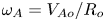$\omega _{A} = V_{A o} /R_o$. This ordering implies a high-$\beta$ scenario $\langle \beta \rangle \sim {O}(\epsilon)$, where the poloidal magnetic field is a fraction of the toroidal one, $B_p / B_{\varphi o} \sim {O}(\epsilon)$, and with a kink-safety factor of ${q_*}\sim {O}(1)$. Here, the kink-safety factor is defined as

(2.11)\begin{equation} q_* = \frac{a B_{\varphi}}{R_o B_p} = \frac{2 {\rm \pi} a^2 B_{\varphi o}}{\mu_o R_o I}, \end{equation}

where $I$ represents the total toroidal current and the other quantities have been defined before. An explicit expression for $\langle \beta \rangle$ is presented later on. As a boundary condition, it is required that the poloidal flux vanishes at the plasma edge,

(2.12)\begin{equation} \varPsi(a,\theta) = 0. \end{equation}

Under these assumptions, the poloidal flux is found to have a simple closed-form analytical expression; it involves Bessel functions of the first and second kind, and the Meijer G-function (López & Guazzotto Reference López and Guazzotto2017). The solution depends on three figures of merit: the kink safety factor ($q{_*}$), which has been introduced in (2.11); a quantity that determines the $\beta$ regime ($\nu$), which is explicitly given in (2.14); and a measure for the mean magnetic shear ($\lambda$), which is implicitly defined by (2.23); the solution is expressed in the generic way,

(2.13)\begin{equation} \varPsi\left(r,\theta \right) = \varPsi_0(r,q_*,\lambda) + \nu \varPsi_1(r,q{_*},\lambda) \cos(\theta) + {O}(\epsilon B_{\varphi o} a^2). \end{equation}

For the convenience of readers, the equilibrium solution for the poloidal flux that was originally constructed by López & Guazzotto (Reference López and Guazzotto2017) is provided in appendix A. In particular, $\varPsi _0$ and $\varPsi _1$ are given in closed form by (A 4) and (A 5), respectively. While (A 5) is a convenient analytical formula, it is observed that it is singular at $r=0$. A new, series-form representation for $\varPsi _1$ that alleviates this issue is presently introduced (A 6).

We emphasize that $\varPsi _0$ and $\varPsi _1$ are both leading-order contributions to the poloidal flux, i.e. $\varPsi _0(r) \sim \varPsi _1(r) \sim {O}(a^2 B_{\varphi o})$. Here, $\nu$ has a dual meaning: it sets the equilibrium $\beta$ regime, and it acts as a coupling coefficient for the poloidal modes in the stability analysis. It is defined as

(2.14)\begin{equation} \nu \equiv \langle \beta \rangle q_*^2 / \epsilon, \end{equation}

where $\langle \beta \rangle$ is obtained as an average over the plasma volume ($V_p$),

(2.15)\begin{equation} \langle \beta \rangle = \frac{2 \mu_o \langle p \rangle}{B_{\varphi o}^2} = \frac{2 \mu_o}{B_{\varphi o}^2} \frac{1}{V_p} \int p \,\textrm{d}^3r. \end{equation}

Despite the fact that the stationary equilibrium solution is formally derived for high-$\beta$ scenarios ($\nu \sim 1$), it is possible to explore low-$\beta$ configurations ($\nu \ll 1$) as well. The expression for the safety factor at the plasma surface ($q_a$),

(2.16)\begin{equation} q_a =\frac{F(\varPsi)}{2 {\rm \pi}} \oint \frac{\textrm{d}l}{R^2 B_p} = \frac{q_*}{\sqrt{1- \nu^2}}, \end{equation}

indicates that the equilibrium possesses the $\beta$-limit,

(2.17)\begin{equation} \nu < 1. \end{equation}

Another key figure of merit is the magnetic shear. This quantity measures the change of the relative orientation of field lines in neighbouring magnetic surfaces. In general, larger shear is related to better stability properties. In low-$\beta$, large aspect ratio configurations, where the poloidal flux is independent of the poloidal angle (to leading order), a simple expression for the magnetic shear is (Freidberg Reference Freidberg2014),

(2.18)\begin{equation} s(r) \equiv \frac{r}{q}\frac{\textrm{d}q}{\textrm{d}r}, \end{equation}

(not to be confused with the entropy free function) where $q(r)$, the safety factor, is defined here as

(2.19)\begin{equation} q(r) \equiv \left( \frac{1}{r B_{\varphi o}} \frac{\textrm{d} \varPsi_0}{\textrm{d}r} \right)^{-1}. \end{equation}

It was determined in López & Guazzotto (Reference López and Guazzotto2017) that $\lambda$, which appears in (2.13), is an auxiliary variable arising during the simplification of the GSB system (see (A 1)), and that it is related to the free coefficients introduced in (2.7)–(2.10) through the transcendental equation,

(2.20)\begin{equation} \lambda = \frac{\nu^2 f(\lambda)^2}{q_*^2\,f_0^2} + \frac{ \varOmega_o^2}{\epsilon^2 \omega_A^2\rho_0}+ f_0\, f_{22}+ \rho_0 h_{11}- \frac{ s_{11} \rho_0^{\gamma}}{\gamma -1}, \end{equation}

here, the leading-order dimensionless density is

(2.21)\begin{equation} \rho_0=\left(\frac{(\gamma -1)h_0}{\gamma s_0}\right)^{1/(\gamma -1)} \end{equation}

and

(2.22)\begin{equation} f(\lambda) \equiv - \frac{2 J_1(\sqrt{\lambda})}{{}_0\tilde{F}_1\left(;3;-\dfrac{\lambda }{4}\right) \sqrt{\lambda }}, \end{equation}

where $_0\tilde {F}_1$ is the regularized confluent hypergeometric function (DLMF 2020, § 15.1). Interestingly, $\lambda$ can be regarded as a measure of the magnetic shear. This is more easily seen by considering a low-$\beta$ approximation. In that regime, the average value of the magnetic shear over the cross-section of the plasma ($A_p$) has a simple form,

(2.23)\begin{equation} \langle s \rangle \equiv \frac{1}{A_p}\int s(r)\,\textrm{d}^2 r= 1 -2 \ln \left(J_1(\sqrt{\lambda })\right) +4 \int_0^{1} \bar{r} \ln \left(J_1 \left( \sqrt{\lambda }\bar{r}\right)\right) \textrm{d}\bar{r} + {O}(\nu). \end{equation}

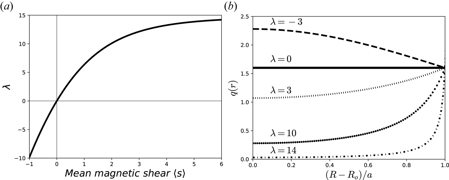
This is to be understood as an implicit definition for $\lambda$ in terms of the magnetic shear: $\lambda = \lambda ( \langle s \rangle)$. Figure 1(a) shows a monotonic dependence between $\langle s \rangle$ and $\lambda$. Positive (negative) values for the average shear correspond to positive (negative) values for $\lambda$. As the magnetic shear increases, $\lambda$ approaches the squared value of a Bessel function's zero (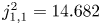$j_{1,1}^2 = 14.682$) asymptotically. As exemplified in figure 1(b) for a low-$\beta$ configuration, the safety factor's concavity changes in accordance with the sign of $\lambda$, being flat when $\lambda$ vanishes.

Figure 1.

(a) The $\lambda$ parameter as a function of the average magnetic shear ($\langle s\rangle$) in a low-$\beta$ approximation. (b) Safety factor in a low-$\beta$ scenario for varying values of $\lambda$.

Additional quantities that will be necessary for the determination of the equilibrium configuration in the vacuum region, as well as to carry out the stability analysis, are the equilibrium mass density and pressure. It is possible to prove that the leading-order mass density is constant,

(2.24)\begin{equation} \rho(r,\theta) = \rho_o + {O}(\epsilon \rho_o), \end{equation}

and that the leading-order kinetic pressure is a flux quantity (López & Guazzotto Reference López and Guazzotto2017). A convenient representation for the pressure, which is not explicitly given by López & Guazzotto (Reference López and Guazzotto2017), is

(2.25)\begin{equation} p(\varPsi) = \frac{B_{\varphi o}}{\mu_o a^2}\langle \beta \rangle q_*f(\lambda) \varPsi + {O}\left(\epsilon \langle \beta \rangle B_{\varphi o}^2/\mu_o \right), \end{equation}

where $f(\lambda)$ has been defined in (2.22). Moreover, in view of the homogeneous Dirichlet condition for the poloidal flux (2.12), it follows that both the kinetic pressure and the angular toroidal velocity vanish at the plasma edge,

(2.26a,b)\begin{equation} p(a,\theta) = 0,\quad \varOmega(a,\theta) = 0. \end{equation}

This leads to convenient simplifications in the evaluation of the boundary conditions at the plasma–vacuum transition.

In regards to the free function $F(\varPsi)$, it is evident that $f_0$ controls the vacuum toroidal magnetic field. The diamagnetic depression of the toroidal magnetic field (or paramagnetic response in the case, e.g. of a reversed field pinch or, possibly, an ohmic tokamak) is determined by $f_1$, $f_2$ and $f_{22}$. In particular, the coefficient $f_1$ is given by

(2.27)\begin{equation} f_1 = \frac{\nu f(\lambda)}{q_* f_0}. \end{equation}

It has been shown that $q_*$, $\epsilon$, $\lambda$ and $\nu$ define the poloidal flux (2.13). Evidently, these parameters should be related to the free coefficients introduced in (2.7)–(2.10). Indeed, (2.20) and (2.27) represent two of these relations. Additionally, it is possible to prove that the following relation holds:

(2.28)\begin{equation} \frac{\sqrt{\lambda} J_0(\sqrt{\lambda}) }{q_* J_1(\sqrt{\lambda})} =-f_0\, f_2-\rho_0 h_1 + \frac{s_1 \rho_0^{\gamma}}{\gamma - 1}. \end{equation}

There are many combinations of the free coefficients that lead to the same form of the poloidal flux. One might think of $q_*$, $\epsilon$, $\lambda$, $\nu$ and $\varOmega _o / \omega _{A}$ as independent dimensionless parameters, and the free coefficients as being implicitly chosen to self-consistent values, albeit this choice is far from being unique. More importantly, it will be proven that the stability of a given configuration depends only on these five independent parameters. Hereafter, $f_0$ is set to unity without loss of generality.

3. Equilibrium model: vacuum

This section's aim is the determination of the inner equilibrium vacuum magnetic field ($\boldsymbol {B}_{V}$). As expected, the vacuum safety factor at the plasma edge is a relevant quantity for stability considerations. This quantity is computed by imposing the continuity of the total pressure, and that of the normal component of the magnetic field, at the plasma–vacuum transition.

While the condition for the continuity of the normal component of the magnetic field, $B_r(a,\theta) = B_{Vr}(a,\theta)$, is trivially satisfied, the condition of the continuity of the total pressure,

(3.1)\begin{equation} p(a,\theta) + \frac{B^2(a,\theta)}{2\mu_o} = \frac{B_V^2(a,\theta)}{2\mu_o}, \end{equation}

is simplified by taking into account that the kinetic pressure vanishes at the plasma edge (2.25 and 2.26a,b). The poloidal component of the vacuum magnetic field is found to be

(3.2)\begin{equation} B_{V \theta}^2(a) = B_{\theta}^2(a) + D \left( 1 - 2 \epsilon\cos{\theta}\right) + {O}(\epsilon^3 B_{\varphi o}^2). \end{equation}

Following Betti (Reference Betti1998), we have introduced the difference

(3.3)\begin{equation} D \equiv \frac{F_a^2(a) - F_{\textrm{Va}}^2(a)}{R_o^2}, \end{equation}

where $F_a$ is obtained from (2.10), $F_a \equiv F(a,\theta) = R_o B_{\varphi o}$, and the free function for the vacuum side evaluated at the interface is $F_{\textrm {Va}} \equiv F_{\textrm {Va}}(\varPsi (a,\theta)) = \textrm {constant}.$ It is observed that $D$ controls the amount of surface current at the plasma–vacuum transition. In many sharp-boundary models (Freidberg & Haas Reference Freidberg and Haas1973, Reference Freidberg and Haas1974; Freidberg & Grossmann Reference Freidberg and Grossmann1975; Betti Reference Betti1998; Fitzpatrick Reference Fitzpatrick2008; Rhodes et al. Reference Rhodes, Cole, Brennan, Finn, Li, Fitzpatrick, Mauel and Navratil2018) surface currents originate from the finite jump in the kinetic pressure at the plasma–vacuum interface. In the present model, which possesses a pressure profile that vanishes at the plasma edge, surface currents are not needed, but can be accommodated; however, for simplicity, we consider the $D =0$ case only. Equation (3.2) may be contrasted with (12) from Betti (Reference Betti1998). The form for the equilibrium pressure in the latter model, $p(R) = p_o \exp [(R^2/R_o^2-1)M^2/2]$, where $M=\varOmega R_o \sqrt {\rho _o/ p_o}$ is the Mach number (up to a $\sqrt {3/5}$ factor), results in an extra factor, $4 \epsilon \mu _o p_o (1+ M^2/2) \cos \theta$, not present in (3.2).

Under these conditions, the vacuum safety factor at the plasma–vacuum transition is given by

(3.4)\begin{equation} q_V(a,\theta) = \frac{a B_{\varphi o}}{R_o B_{V \theta}(a,\theta)} = \frac{ q_*}{ 1 + \nu \cos{\theta} }. \end{equation}

Its average value at the plasma edge is

(3.5)\begin{equation} \langle q_V \rangle_a = \frac{1}{2 {\rm \pi}} \int_0^{2 {\rm \pi}} \frac{a B_{\varphi o} \,\textrm{d}\theta}{R_o B_{V \theta}(a,\theta)} = \frac{q_*}{\sqrt{1 - \nu^2} } = q_a. \end{equation}

Finally, a quantity of interest for stability considerations is

(3.6)\begin{equation} \left \langle \frac{1}{q_V^2} \right \rangle_a \equiv \frac{1}{2 {\rm \pi}} \int_0^{2 {\rm \pi}} \frac{\textrm{d}\theta}{q_V^2(a,\theta)} = \frac{2 + \nu^2}{2 q_*^2} . \end{equation}

This expression is useful to evaluate the kink-mode drive for instabilities in § 7.

4. Frieman–Rotenberg formulation

For the linear stability analysis we employ the well known formulation by Frieman & Rotenberg (Reference Frieman and Rotenberg1960). In this formulation, perturbed quantities are expressed as functions of the quasi-Lagrangian plasma displacement ($\boldsymbol {\xi }$). For normal modes of the form

(4.1)\begin{equation} \boldsymbol{\xi}(\boldsymbol{r},t) = \hat{\boldsymbol{\xi}}(R,Z) \exp({-\textrm{i}(\omega t+n \varphi) }), \end{equation}

the spectral equation for axisymmetric systems, in the case of plasmas with toroidal rotation only, reduces to

(4.2)\begin{equation} \tilde{\boldsymbol{F}}(\hat{\boldsymbol{\xi}}) = -\rho \bar{\omega}^2 \hat{\boldsymbol{\xi}} - 2 \textrm{i} \rho \bar{\omega} \varOmega \hat{\boldsymbol{e}}_Z \times \hat{\boldsymbol{\xi}} + (2 \rho R \varOmega \hat{\boldsymbol{\xi}} \boldsymbol{\cdot} \boldsymbol{\nabla} \varOmega) \hat{\boldsymbol{e}}_R - \tilde{\rho} \varOmega^2 R \hat{\boldsymbol{e}}_R, \end{equation}

where the Doppler-shifted frequency is given by

(4.3)\begin{equation} \bar{\omega} \equiv \bar{\omega}(R,Z) = \omega + n \varOmega(R,Z). \end{equation}

Hereafter, the ‘hats’ will be dropped; it should be understood that all perturbed quantities, and in particular the displacement vector, are time-independent. Utilizing the axisymmetric condition, it is possible to express the force operator as

(4.4)\begin{equation} \tilde{\boldsymbol{F}}(\boldsymbol{\xi}) = \frac{1}{\mu_o} \left\{ \tilde{\boldsymbol{B}}_p \boldsymbol{\cdot} \boldsymbol{\nabla} \boldsymbol{B} + \boldsymbol{B} \boldsymbol{\cdot} \boldsymbol{\nabla} \tilde{\boldsymbol{B}}_p - \frac{2 B_{\varphi} \tilde{B}_{\varphi}}{R} \hat{\boldsymbol{e}}_R + \left[ \frac{B_{R} \tilde{B}_{\varphi}}{R} + \boldsymbol{B} \boldsymbol{\cdot} \boldsymbol{\nabla} \tilde{B}_{\varphi} \right] \hat{\boldsymbol{e}}_\varphi \right\} - \boldsymbol{\nabla} \tilde{\varPi}. \end{equation}

This form of the force operator facilitates the computation of the plasma–vacuum boundary condition in § 7. The perturbed magnetic field has been decomposed into its poloidal and toroidal components,

(4.5)\begin{equation} \tilde{\boldsymbol{B}} = \tilde{\boldsymbol{B}}_p + \tilde{\boldsymbol{B}}_{\varphi}, \end{equation}

the remaining perturbed quantities are

(4.6)\begin{gather} \tilde{p} = -\gamma p \boldsymbol{\nabla} \boldsymbol{\cdot} \boldsymbol{\xi} - \boldsymbol{\xi} \boldsymbol{\cdot} \boldsymbol{\nabla} p, \end{gather}

(4.7)\begin{gather}\tilde{\rho} = - \boldsymbol{\nabla}\boldsymbol{\cdot} (\rho \boldsymbol{\xi}) = - \rho \boldsymbol{\nabla} \boldsymbol{\cdot} \boldsymbol{\xi} - \boldsymbol{\xi} \boldsymbol{\cdot} \boldsymbol{\nabla} \rho, \end{gather}

(4.8)\begin{gather}\boldsymbol{\tilde{B}} = \boldsymbol{\nabla} \times \left( \boldsymbol{\xi} \times \boldsymbol{B} \right), \end{gather}

where the total pressure is given by the sum of the kinetic and magnetic contributions,

(4.9)\begin{equation} \tilde{\varPi} \equiv \tilde{p} + \frac{B \tilde{B}_{\parallel}}{\mu_o}, \end{equation}

here, $\parallel$ stands for a component parallel to the equilibrium magnetic field.

5. The Shear–Alfvén Law

The Shear–Alfvén law is obtained from the axisymmetric form of the momentum equation. This can be accomplished by either taking $\hat {\boldsymbol {e}}_{\varphi } \boldsymbol {\cdot } \boldsymbol {\nabla } \times$(4.2) and, subsequently, eliminating the $\partial _Z (B_{\varphi } \tilde {B}_{\varphi })$ term from the $Z$ component of the momentum equation, as done by Betti (Reference Betti1998) or, equivalently, by taking $\boldsymbol {\nabla } \varphi \boldsymbol {\cdot } \boldsymbol {\nabla } \times [R^2$ (4.2)$]$. Loosely speaking, the resultant equation ($\mathcal {M}=\mathcal {L}$) consists of a ‘magnetic part’ ($\mathcal {M}$), which depends on the perturbed poloidal magnetic field; and of an ‘inertial part’ ($\mathcal {L}$), which depends on the perturbed density, velocity, and kinetic pressure. These contributions are

(5.1)\begin{equation} \mathcal{M} = -\boldsymbol{\nabla} \varphi \boldsymbol{\cdot} \boldsymbol{\nabla} \times \left[ R^2 \left[ \tilde{\boldsymbol{B}}_p \times J_\varphi \hat{\boldsymbol{e}}_\varphi + \frac{ \boldsymbol{B}}{\mu_o}\times ( \boldsymbol{\nabla} \times \tilde{\boldsymbol{B}}_p) \right] \right], \end{equation}

where $J_{\varphi }$ is the equilibrium current density in the toroidal direction, and

(5.2)\begin{equation} \mathcal{L} = -\boldsymbol{\nabla} \boldsymbol{\cdot }(\rho \bar{\omega}^2 R \boldsymbol{\xi} \times \hat{\boldsymbol{e}}_\varphi) + \partial_{Z} [2 \textrm{i} \rho \bar{\omega} \varOmega R \xi_\varphi + 2 \rho R^2 \varOmega \boldsymbol{\xi} \boldsymbol{\cdot} \boldsymbol{\nabla} \varOmega - \tilde{\rho} \varOmega^2 R^2-2 \tilde{p}]. \end{equation}

One of the main differences between the stability analysis presented here and that developed in Betti (Reference Betti1998) for a configuration with a solid angular rotation profile, is that the flow shear drive 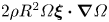$2 \rho R^2 \varOmega \boldsymbol {\xi } \boldsymbol {\cdot } \boldsymbol {\nabla } \varOmega$ is absent in the latter model.

Even though the magnetic ($\mathcal {M}$) and inertial ($\mathcal {L}$) expressions are exact for axisymmetric configurations, equilibrium quantities are known to leading order in the inverse aspect ratio only. Accordingly, the stability analysis in this work can be accurate to leading order at most. The following stability analysis is based on the work by Betti (Reference Betti1998) for a configuration with rigid rotation.

6. Eigenvalue system of ODEs

The goal of this section is to obtain the $m$-th Fourier component of the Shear–Alfvén law. Perturbed quantities ($\tilde {f}$) are expressed as a superposition of poloidal modes in the usual way,

(6.1)\begin{equation} \tilde{f}(r,\varphi,\theta)= \sum_{m=-\infty}^{\infty} f_m(r) \exp({\textrm{i} (m\theta - n \varphi)}). \end{equation}

The calculation proceeds by introducing a stream function representation for the plasma displacement. The feasibility of this representation derives from the fact that the perturbed toroidal magnetic field is smaller than the poloidal one (in terms of the inverse aspect ratio). Following Waelbroeck (Reference Waelbroeck1996), we write 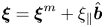$\boldsymbol {\xi } = \boldsymbol {\xi }^m + \xi _\parallel \hat {\boldsymbol {b}}$, where $\boldsymbol {\nabla } \varphi \boldsymbol {\cdot } \boldsymbol {\xi }^m= 0$. A straightforward manipulation shows that, for our equilibrium configuration, 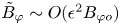$\tilde {B}_\varphi \sim {O}{(\epsilon ^2 B_{\varphi o})}$, and this leads (Waelbroeck Reference Waelbroeck1996) to a stream function representation for the meridian plasma displacement component, $\boldsymbol {\xi }^m = F^{-1}R^2 \boldsymbol {\nabla } U \times \boldsymbol {\nabla } \varphi + {O}{(\epsilon ^2 a)}$, where $U$ is the stream function, as well as a potential representation for the perturbed magnetic field, $\boldsymbol {\tilde {B}} = \boldsymbol {\nabla } \tilde {\varPsi } \times \boldsymbol {\nabla } \varphi + {O}{(\epsilon ^2 B_{\varphi o})}$, where we have introduced a stream function for the perturbed poloidal magnetic flux as $\tilde {\varPsi } \equiv F^{-1}R^2 \boldsymbol {B} \boldsymbol {\cdot } \boldsymbol {\nabla } U$.

The potential representation for the perturbed magnetic field is readily employed in the simplification of the magnetic contribution in the Shear–Alfvén law, yielding

(6.2)\begin{equation} \mathcal{M}_m = \left( \frac{ \textrm{i} B_{\varphi o}}{ r \mu_o R_o }\right) \left\{ \left( -m h_m + \frac{1}{r}\frac{\textrm{d}}{\textrm{d}r}\left[ r^3 \frac{\textrm{d}\mu}{\textrm{d}r}\right]\right)\frac{m \tilde{\varPsi}_m}{r} + h_m \frac{\textrm{d}}{\textrm{d}r}\left[ r \frac{\textrm{d} \tilde{\varPsi}_m}{\textrm{d}r}\right]\right\}\left( 1 + {O}{(\nu)}\right), \end{equation}

where

(6.3)\begin{equation} \mu(r) = 1/ q(r) \end{equation}

and

(6.4)\begin{equation} h_m(r) = n - m \mu(r). \end{equation}

We have chosen to express $\mathcal {M}_m$ to leading order in $\nu$. We recall that $\nu \sim {O}(1)$ by construction, but this quantity is always below unity, in accordance with the equilibrium $\beta$-limit (2.17). In this work, $\nu$ is regarded as an expansion parameter. In recognition of the non-circular nature of magnetic flux surfaces in high-$\beta$ configurations (characterized here by $\nu$), other works ( Ito & Nakajima (Reference Ito and Nakajima2019), and references therein) have constructed magnetic flux coordinates in the presence of flows as the basis for stability analysis.

The computation continues by imposing incompressibility as follows:

(6.5)\begin{equation} \boldsymbol{\nabla} \boldsymbol{\cdot} \boldsymbol{\xi} = 0. \end{equation}

An a posteriori justification for this assumption has been provided by (Betti Reference Betti1998, appendix C) in the context of a rigid rotating scenario. The validity condition for (6.5) turns out to be $\bar {\omega }^2/\omega _s^2 \ll 1$ where $\omega _s = V_s /R_o$ is the sound frequency (here, $V_s = \sqrt { \gamma p_o /\rho _o}$ is the sound speed). In the present work, $\varOmega ^2 /\omega _{s}^2 \sim {O}(\epsilon) \ll 1$ by construction. Likewise, the growth rates of the resistive and ideal modes under consideration satisfy the validity condition (see § 9). In related work, the implications of the incompressibility constraint on the stability of the $m = n =1$ internal kink mode have been extensively analysed by Wahlberg & Bondeson (Reference Wahlberg and Bondeson1997). An a posteriori justification of (6.5) might be invoked for the present work as well. The incompressibility condition leads to a simple relation between the $m$-th Fourier component for the perturbed poloidal flux ($\tilde {\varPsi }_m$), and for the radial plasma displacement ($\xi _m$),

(6.6)\begin{equation} \tilde{\varPsi}_m = B_{\varphi o} \frac{r h_m \xi_m}{m} \left( 1 + {O}{(\nu)}\right). \end{equation}

We now turn to the inertial term, given by (5.2). It is observed that the perturbed plasma density ($\tilde {\rho }$) is zero to leading order in the inverse aspect ratio. This follows from the fact that the leading-order density is constant (2.24), and the incompressibility condition. A beneficial consequence of the equilibrium model under consideration is that, as long as $\nu \gg \epsilon$, the Doppler, the Coriolis and the centrifugal contributions that appear in the Shear–Alfvén law, are one order (in $\epsilon$) smaller than flow shear effects and may be neglected. Under this assumption, a straightforward algebraic manipulation leads to the $m$-th Fourier component of the inertial term,

(6.7)\begin{align} \mathcal{L}_m &=\left( \frac{-R_o\rho_o}{ i m r}\right) \left\{\frac{1}{r}\frac{\textrm{d}}{\textrm{d}r}\left[ \left( \omega^2 r^3 - K a r^2\right)\frac{\textrm{d} \xi_{m}}{\textrm{d}r}\right] \right. \nonumber\\ &\quad \left. -\left[ (m^2-1) \left( \omega^2- a \frac{\textrm{d}K}{\textrm{d}r} \right)\right] \xi_{m} \right\}\left( 1 + {O}{(\epsilon)}\right) \nonumber\\ &\quad -\textrm{i}\left\{\frac{ \left[(m-1) \tilde{p}_{m-1}+(m+1) \tilde{p}_{m+1}\right]}{r}+ \left[\frac{\textrm{d}\tilde{p}_{m+1}}{\textrm{d}r}- \frac{\textrm{d}\tilde{p}_{m-1}}{\textrm{d}r}\right]\right\}. \end{align}

We have introduced the function

(6.8)\begin{equation} K(r) \equiv \frac{\nu \varOmega_o^2}{\epsilon} \frac{\varPsi_0(r) \varPsi_1(r)}{a^4 B_{\varphi o}^2}. \end{equation}

It is recalled that $\varPsi _0(r) \sim \varPsi _1(r) \sim {O}(a^2 B_{\varphi o})$ are the contributions of the equilibrium poloidal flux in (2.13); it follows that $K(r)\sim {O}(\nu \varOmega _o^2 / \epsilon) \sim {O}(\nu \epsilon \omega _A^2)$. Here, $K(r)$ captures the flow shear drive for instabilities. Interestingly, this is a high-$\beta$ toroidal effect, which disappears in the cylindrical limit ($\nu \rightarrow 0$).

Direct inspection of the linearized projection of the momentum equation along the magnetic field inform us that the flow-dependent terms in it are smaller than the flow shear drive in (6.7) (the $K$-term) by a factor ${\sim }\epsilon /\nu \ll 1$; hence, the former contributions are neglected. This results in a simple expression for the side bands of the perturbed pressure ($\tilde {p}_{m\pm 1}$) as a function of the parallel plasma displacement which is substituted back into (6.7).

In writing down the $m$-th Fourier component of the inertial term ($\mathcal {L}_m$), we have neglected poloidal modes other than the principal. It is interesting to point out that while pressure gradient mode coupling is not captured across the plasma column in the stability analysis of Betti (Reference Betti1998) due to the features of the equilibrium considered there, here, it enters as an effect of order ${\sim }O(\nu f(\lambda)/ q_*)$, where $f(\lambda) \sim {O}(1)$ has been defined in (2.22). Comparing the pressure gradient mode coupling ordering with the flow shear contribution (6.8) reveals that the former is dominant by a factor of $\epsilon$. 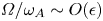This is so because 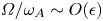$\varOmega / \omega _A \sim {O}(\epsilon)$ by construction. However, in order to make analytical progress, pressure gradient mode coupling across the plasma column is neglected in our work. In contrast, the eigenmode equation derived in Chapman et al. (Reference Chapman, Walkden, Graves and Wahlberg2011) and Wahlberg et al. (Reference Wahlberg, Graves and Chapman2013), for low-$\beta$ plasmas with $\varOmega / \omega _A \sim {O}(\epsilon)$, retains equilibrium pressure gradient effects. In Betti (Reference Betti1998), harmonic coupling at the ODE level corresponds to small corrections of order ${\sim }{O}(\bar {\omega }^2/\omega _A^2)$ and is disregarded. In addition to implementing this approximation in our work, we also neglect mode coupling induced by the diffuse nature of the angular toroidal frequency. The interaction between different poloidal modes, which is characterized by $\nu$, is retained at the plasma–vacuum transition only.

We are finally in a position to construct the $m$-th governing eigenmode ODE. Following Betti (Reference Betti1998) we introduce the functions

(6.9)\begin{equation} Y_m^2(r)\equiv r\frac{\textrm{d}}{\textrm{d}r}\left[\frac{(m-1)\omega^2}{ h_{m+1}^2}\right]-r\frac{\textrm{d}}{\textrm{d}r}\left[\frac{(m+1)\omega^2}{ h_{m-1}^2}\right] \end{equation}

and

(6.10)\begin{equation} \varGamma_m^2(r) \equiv \omega^2\left( 1 + \frac{1}{h_{m+1}^2} + \frac{1}{h_{m-1}^2} \right). \end{equation}

Equations (6.9) and (6.10) differ from (31) and (32) of Betti (Reference Betti1998) in that the former pair does not capture centrifugal and Coriolis effects but the latter pair does. By equating the inertial term, from (6.7), with the magnetic term, from (6.2), we obtain

(6.11)\begin{align} &\frac{1}{r}\frac{\textrm{d}}{\textrm{d}r} \left[ ( [ \varGamma_m^2 - \omega_{A}^2h_{m}^2]r^3 -a r^2 K ) \frac{\textrm{d} \xi_m}{\textrm{d}r} \right] \nonumber\\ &\quad -\left[(m^2-1)\left( \varGamma_m^2 - \omega_{A}^2 h_m^2 - a\frac{ \textrm{d}K}{\textrm{d}r} \right) + Y_m^2 \right] \xi_m = 0. \end{align}

Equation (6.11) should be compared with (38) of Betti (Reference Betti1998). It is observed that in the vanishing flow limit these equations formally agree. However, since profiles for the safety factor differ between the models, so do the $h_m(r)$ contributions in the eigenmode equations. In Betti (Reference Betti1998), there are two regions of interest: a central region with a constant safety factor and a thin region near the edge with a quadratic safety factor. Our model encompasses both possibilities: a constant safety factor is obtained when there is no magnetic shear ($\lambda = 0$) and a quadratic safety factor in the neighbourhood of the plasma edge is obtained by setting $\lambda = 5.78319$. Besides the eigenmode equation (6.11), the eigenvalue problem requires the specification of appropriate boundary conditions. They are supplied in the next section.

7. Boundary conditions and wall effects

Boundary conditions are imposed at the plasma–vacuum interface, and at the outer material wall. Since the vacuum magnetic field is expressible as the gradient of a scalar potential ($\tilde {\boldsymbol {B}}_V = \boldsymbol {\nabla } \tilde {V}$), the condition for the continuity of the perturbed total pressure at the plasma–vacuum interface may be written as

(7.1)\begin{equation} \tilde{\varPi}_m(a) - \left.\left[\left[ \xi_r \frac{\partial}{\partial r}\left(p + \frac{B^2}{2 \mu_o} \right) \right]\right]_m \right\vert_a = \left.\left[ \frac{\boldsymbol{B}_V \boldsymbol{\cdot} \boldsymbol{\nabla} \tilde{V}}{\mu_o} \right]_m \right\vert_a. \end{equation}

Here, $[[~.~]]_m |_a$ represents the $m$-th Fourier component of the jump of a given quantity at the plasma edge. After a standard algebraic manipulation (see appendix B) it is possible to recast the boundary condition (7.1) in a way that explicitly depends on the Fourier components of the radial plasma displacement. In the final formulation, (B 9), Fourier components of the radial plasma displacement are coupled together by means of the $\nu$ coefficient, as defined in (2.14). Equation (B 9) incorporates the wall position ($r_w$) and wall resistive time ($\tau _w = \mu _o \,\textrm {d} r_w /\eta _w$) through the function $\hat {\sigma }_l=\hat {\sigma }_l(\omega ,\tau _,r_w)$, as defined by (B 7).

Stability boundaries for cylindrical plasmas with no walls can be recovered from the eigenmode equation (6.11) and boundary conditions (B 9). This is accomplished by taking the vanishing $\nu$ limit, neglecting the $h_{m \pm 1}$ coupling terms, and setting $\hat {\sigma }_l=1$. In this limit, the model under consideration reduces to the pressureless configuration with a flat current profile and a jump at the plasma edge, which has been thoroughly studied in the context of the straight-tokamak approximation by means of the energy principle (Freidberg Reference Freidberg2014). For that model, it is concluded that the condition for instability is

(7.2)\begin{equation} m-1 < n q_a < m. \end{equation}

8. Solution technique: matrix-generated dispersion relation and multidimensional shooting method

For a collection of side bands $M_{\min } \leq m \leq M_{\max }$ ($m \neq 0$), the eigenvalue problem consists in solving $M_{\max } -M_{\min } + 1$ eigenmode ODEs (6.11), and determining the corresponding eigenfrequency $\omega$, so that the set of coupling boundary conditions (B 9) is satisfied.

Harmonic contributions for the plasma displacement are required to be regular at ${r=0}$. In this respect, it is observed that the governing ODE possesses a regular singularity at the origin, a situation which is typical. Ordinarily, the removal of the singularity is accomplished by expanding the coefficients of (6.11) as a power series centred at $r =0$. An illustration of this procedure can be seen, for example, in Hazeltine & Meiss (Reference Hazeltine and Meiss2003). However, for the present model, there is a caveat: the closed-form analytic expression for $\varPsi _1$ (A 5), introduced by López & Guazzotto (Reference López and Guazzotto2017), which enters into the picture through the flow shear contribution (6.8) is undefined at $r = 0$, specifically,

(8.1)\begin{equation} \lim_{r\to0}\varPsi_1(r) = 0,\quad \text{but}\ \varPsi_1(0) = \infty. \end{equation}

In order to deal with this unphysical limitation a new representation of $\varPsi _1$, one that is $\mathcal {C}^\infty$ across the whole plasma column (including $r=0$), is constructed in appendix A (A 6). Once the $\varPsi _1$ part in the flow shear contribution is understood to be expressed in terms of (A 6), it is straightforward to reduce (6.11) into an equidimensional ODE in the neighbourhood of $r =0$, and prove that the behaviour for the plasma displacement around the origin is the expected one,

(8.2)\begin{equation} \xi_{m} = c_{m} r^{-1+|m|}, \end{equation}

where, $c_m$ are arbitrary complex constants.

Given a set of $c_m$, one of these constants can be chosen in an arbitrary way without loss of generality (say, the one corresponding to $m = M_{\max }$). Thus, the eigenvalue problem consists of determining $M_{\max } -M_{\min } + 1$ complex numbers: $\{\omega , c_{M_{\min }}, c_{M_{\min }+1},\ldots , c_{M_{\max }-1}\}$ consistent with boundary conditions. In regards to the numerical integration, it is carried out starting at a point $r_o$ (with $0 < r_o \ll a$) where continuity of the plasma displacement and its derivative, as computed from (8.2), are imposed. Since the closed-form analytical expression for $\varPsi _1$ (A 5) is regular in the interval $[r_o, a]$, it is the one employed for numerical integration. In this way, the stability eigenvalue problem has been recast as a multidimensional shooting method.

In a multidimensional shooting method, good initial guesses are critical in order to achieve convergence. It is fortunate that a robust method to compute such initial guesses can be developed for the problem at hand. Despite the fact that the governing ODE must be solved numerically (in general), static plasmas with no magnetic shear admit a solution identical to (8.2), not only at the origin's neighbourhood but across the whole plasma column. In this regime, the set of boundary conditions reduces to a linear system for the mode amplitudes ($c_m$), and its determinant leads to the system's dispersion relation, which is solvable by a root-finding method over the complex plane. Therefore, in this regime, the complete set of eigenvalue/eigenvectors pairs is computable with no uncertainty (up to numerical errors); they constitute excellent initial guesses. Then, by progressively changing equilibrium parameters, it is possible to explore regions of parameter space with finite values for the velocity and the magnetic shear.

9. The stability of $n=1$ modes surrounded by ideal and resistive walls

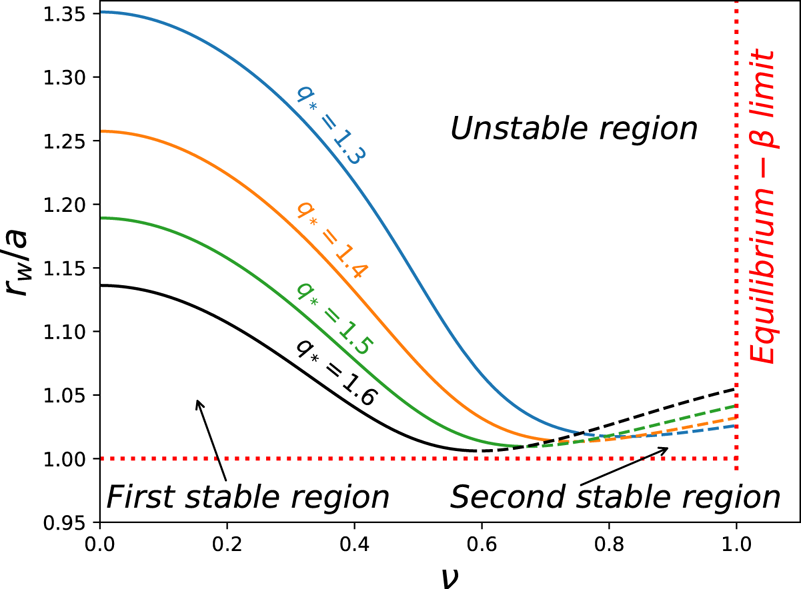
Stability boundaries for static plasmas with no magnetic shear surrounded by an ideal wall are shown in figure 2. Plasmas with vanishing magnetic shear admit a simple equilibrium solution,

(9.1)\begin{equation} \lim_{\langle s \rangle \rightarrow 0} {\varPsi(r,\theta)} = \frac{1}{2 {q_* a^2}}[(r^2 -a^2) + \nu (r^3 - ra^2) \cos(\theta)], \end{equation}

which corresponds to the high-$\beta$ static model developed by Freidberg (Reference Freidberg2014, equation (6.103)). The computation of figure 2 utilizes (9.1) for the equilibrium solution instead of the general equations (A 4) and (A 5), which are valid for an arbitrary value of the magnetic shear. Stability curves are found by fixing the kink-safety factor and plasma pressure ($\nu$), progressively increasing the wall radius and computing, at each $(\nu , r_w)$ point, the complete set of eigenvector/eigenvalue pairs by solving the matrix-generated dispersion relation. Marginal stability is reached when the growth rate of the fastest-growing mode vanishes ($\omega _I \equiv \textrm {Im}\{\omega \}=0$). Stability boundaries are found for the $n = 1$ toroidal mode by considering a narrow poloidal spectrum of only five modes, $m = 1, 2, 3, 4, 5$. In contrast, the stability of highly shaped configurations has been studied in the past by retaining the coupling of up to 45 poloidal modes (Rhodes et al. Reference Rhodes, Cole, Brennan, Finn, Li, Fitzpatrick, Mauel and Navratil2018).

Figure 2.

Marginal stability boundaries against $n = 1$ external kink modes for a static plasma with zero magnetic shear, an ideal wall and varying values of the kink-safety factor. The $r_w/a = 1$ horizontal line corresponds to the situation in which the wall is positioned at the plasma edge. In the $\langle s \rangle = 0$, $\langle \varOmega \rangle = 0$ configuration considered here, the diffuse model simplifies to the high-$\beta$ model of Freidberg (Reference Freidberg2014).

The condition for instability (7.2) indicates that for $n=1$ the plasma is unstable in the entire range $0 \leq q_a\leq \infty$. As illustrated in figure 2, for the stabilization of this ideal-plasma external kink mode (IPKM) it is necessary to bring the wall from infinity to a finite position near the plasma. Our study focuses on external kink modes when there are no resonant surfaces located inside the plasma. In principle, to avoid the onset of the $m/n=2/1$ tearing mode an upper limit $q_a < 2$ should be imposed, which (according to (2.16)) would translate into an upper bound for $\nu$. However, despite the fact that toroidal effects are considered in the stability analysis, resonances enter as if the configuration was cylindrical (see (2.19), (6.3) and (6.4)) and this $\nu$-dependent upper limit is not captured by the stability model. In any case, in order to keep track of this approximation, the dashed part of the marginal stability curves in figure 2 indicate that these critical values for $\nu$ have been surpassed. Stability curves are computed up to the equilibrium $\beta$-limit $\nu < 1$ (2.17).

As in other stability analyses (Betti Reference Betti1998; Rhodes et al. Reference Rhodes, Cole, Brennan, Finn, Li, Fitzpatrick, Mauel and Navratil2018), a second region of stability is found in the high-$\beta$ regime for the present model. Among the possibilities shown in figure 2, it would be desirable to operate at $q_*=1.6$, since this option offers more ‘high-$\beta$ room’ than the others ($q_* = 1.3, 1.4, 1.5$). At a fixed wall radius, accessing a high-$\beta$ regime is accomplished by transiting across a region of unstable $\beta$. 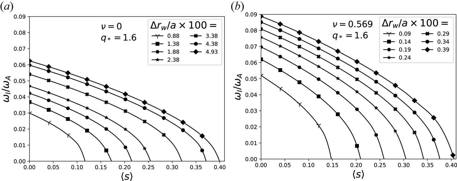Hypothetically, this transition could be aided with the addition of magnetic shear ($\langle s \rangle$). It is recalled that the equilibrium solution under consideration is able to accommodate changing values for the mean magnetic shear, as explained through (2.18)–(2.23) and shown in figures 1(a) and 1(b). Figure 3(b) illustrates the suppression of the fastest-growing mode as the average magnetic shear is increased at varying distances above (${\rm \Delta} r_w/a$) the marginal stability wall position when it is closest to the plasma edge (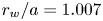$r_w/a = 1.007$); a situation which occurs when the coupling parameter is $\nu =0.596$ (as can be seen from figure 2). Starting at 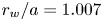$r_w/a = 1.007$ and $\langle s \rangle = 0$, we move upward into the unstable regime a distance ${\rm \Delta} r_w/a$, this results in the onset of finite growing IPKMs; however, a subsequent application of a positive magnetic shear is able to completely suppress the instabilities. Unfortunately, despite the fact that the addition of magnetic shear raises the stability boundaries, this effect is small at the global minimum of the $q_*=1.6$ curve. Indeed, for a mean magnetic shear of $\langle s \rangle \sim 0.4$, the stability boundary would move up around ${\rm \Delta} r_w = 0.39$ cm in a plasma with a minor radius of one metre. In contrast, at zero $\beta$, the same strength for the magnetic shear raises the stability boundary approximately ${\rm \Delta} r_w = 4.93$ cm (see figure 3a). This indicates that magnetic shear stabilization is more effective in the low-$\beta$ regime. For the $q_*=1.6$ case, increasing the value of the magnetic shear above $\langle s \rangle = 0.48$ results in internal resonances; it is the purpose of future work to determine the effect of magnetic shear in those circumstances.

Figure 3.

Magnetic shear stabilization of the $n=1$ mode for a plasma surrounded by an ideal wall and with $q_*=1.6$ at (a) zero pressure ($\nu =0$) and (b) finite pressure ($\nu =0.596$). In the vanishing magnetic shear scenario ($\langle s \rangle = 0$), figure 2 indicates that the marginal wall position for case (a) is $r_w/a = 1.136$, while that for case (b) is $r_w/a = 1.007$. Starting at those positions, we travel a distance ${\rm \Delta} r_w/a$ upwards into the unstable regime without increasing the magnetic shear; this results in finite growth rates ($\omega _I/\omega _A$). At those fixed locations, a subsequent increase in the magnetic shear leads to the stabilization of the plasma column.

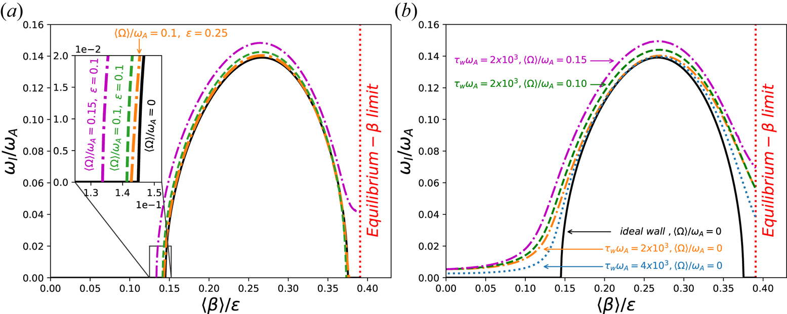
The consequence of adding a finite mild flow shear drive in the presence of ideal and resistive walls is exemplified in figure 4 for equilibria with angular frequencies ($\langle \varOmega \rangle$) of a considerable fraction of the Alfvén frequency. Here, $\langle \varOmega \rangle$ is defined as an average over the plasma volume,

(9.2)\begin{equation} \langle \varOmega \rangle = \frac{1}{V_p} \int \varOmega(\varPsi) \,\textrm{d}^3r = -\frac{ \varOmega_o \, _0\tilde{F}_1\left(;3;-\dfrac{ \lambda }{4}\right)}{2 q_* \, _0\tilde{F}_1\left(;2;-\dfrac{ \lambda }{4}\right)}, \end{equation}

where $\lambda$ is, in turn, given by (2.23). For a fixed wall radius of $r_w/a = 1.05$ and a kink-safety factor of $q_* = 1.6$, figure 4(a) illustrates the onset of IPKMs as the pressure increases and the subsequent transition into the second stability region. Meanwhile, figure 4(b) exemplifies the onset of ideal-plasma resistive wall modes (IPRWMs). It is well understood that IPRWMs eliminate the stabilizing influence of the wall on times comparable to the diffusion time, which we have chosen as $\tau _w \omega _A= 2 \times 10^3$ and $\tau _w \omega _A= 2 \times 10^4$. The IPRWMs corresponding to static plasmas in figure 4(b) are in qualitative agreement with figure 5 of Betti (Reference Betti1998), which employs $\tau _w \omega _A= 2 \times 10^4$, and with figures 2 and 3 of Rhodes et al. (Reference Rhodes, Cole, Brennan, Finn, Li, Fitzpatrick, Mauel and Navratil2018), where $\tau _w \omega _A= 10^3$. It has been pointed out that at zero $\beta$ the model under consideration is unstable if the wall is at infinity (7.2), accordingly, figure 4(b) shows residual IPRWMs at zero $\beta$. On the contrary, the models considered by Betti (Reference Betti1998) and by Rhodes et al. (Reference Rhodes, Cole, Brennan, Finn, Li, Fitzpatrick, Mauel and Navratil2018) are stable below critical $\beta$ values, and it is the purpose of those articles to determine the degree to which rigid rotation can increase these $\beta$-limits. In the absence of rotation, resistive wall tearing modes constitute the least stable modes, consequently, plasma resistivity should be taken into account (Betti Reference Betti1998; Rhodes et al. Reference Rhodes, Cole, Brennan, Finn, Li, Fitzpatrick, Mauel and Navratil2018). Presently, our work considers ideal plasmas only, it is the aim of future work to incorporate plasma resistivity.

Figure 4.

Comparison of growth rates of the $n = 1$ mode for plasmas with diffuse toroidal rotation in the presence of (a) ideal walls and (b) resistive walls. The comparison is performed at varying rotating frequencies of a significant fraction of the Alfvén frequency. Here, $\langle \varOmega (\varPsi) \rangle$ represents the average toroidal rotation over the plasma volume. In all cases $q_*=1.6$, $\langle s\rangle = 0$ and $r_w/a = 1.05$. In panel (b) $\epsilon = 0.1$.

The combined effect of resistivity and flow shear results in a magnification of the growth rates for all $\beta$ (see figure 4b). Figure 4(a) illustrates that IPKMs growth rates increase with rotation, and that $\beta$-limits decrease with it. It is recalled that in the present stability analysis flow shear dominates over all other velocity dependent contributions as long as $\nu \gg \epsilon$. In figure 4(a), this assumption is better satisfied for the $\epsilon =0.1$ case than for the more realistic $\epsilon =0.25$ scenario; however, it is beneficial to be able to visualize the effect of flow shear alone, even if that is possible in this small $\epsilon$-limit only. When $\nu$ and $\epsilon$ are comparable, centrifugal and Coriolis contributions should be retained.

In order to compare the effect of flow for the diffuse scenario with a rigid rotation configuration, the model developed by Betti (Reference Betti1998) is reconsidered. In the sharp-boundary formalism with a rigid angular toroidal frequency introduced by Betti (Reference Betti1998), the plasma column is composed of an inner region with a constant safety factor (‘the current channel’) and a thin outer region where the safety factor grows quadratically (‘the plasma edge’). Due to the fact that our model is able to accommodate a flat safety factor ($\langle s \rangle = 0$) we opt for discarding the plasma edge from the sharp-boundary model. The removal of the plasma edge is accomplished by a straightforward modification of the boundary conditions given by equation (67) from Betti (Reference Betti1998). 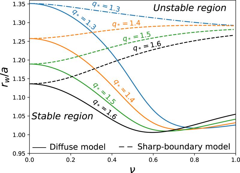In the vanishing flow limit, the remaining differences between the sharp boundary and diffuse models are due to high-$\beta$ terms in the boundary conditions: the ballooning and the kink mode drives differ, and the $\mu _1$ toroidal contribution (B 2) is unique to the diffuse model in this work. For static plasmas, figure 5 illustrates marginal stability curves for both scenarios. As predicted, the models agree in the vanishing $\beta$-limit but strongly differ at higher $\beta$.

Figure 5.

Marginal stability boundaries against $n = 1$ external kink modes for static plasmas with ideal walls and varying values of the kink-safety factor. The solid curves correspond to our model in the case of a constant safety factor ($\langle s \rangle =0$ and $q_* = q_a$), these stability curves are the same as in figure 2, but are replotted here to ease their comparison with the sharp-boundary model. The dashed lines correspond to the sharp-boundary model introduced in Betti (Reference Betti1998) but with a constant safety factor across the whole plasma column, i.e. the so-called ‘plasma edge’: a region where the safety factor grows quadratically, has been self-consistently removed from that model. In the latter model, $\langle q_V \rangle _a$ is an independent variable. Here, it has been chosen as $\langle q_V \rangle _a = q_a$ in order to mimic (3.5), which is valid for the diffuse model.

A meaningful comparison of the effect of flow between the diffuse and sharp-boundary models should be performed in the low-$\beta$ regime, yet, the flow shear drive for instabilities is a high-$\beta$ toroidal effect that vanishes in the cylindrical limit (6.8). Thus, we are led to compare the effect of flow in situations where static scenarios significantly differ. The comparison is performed at $\nu = 0.4$, for a plasma with $\epsilon = 0.1$ (so that the validity condition $\nu \gg \epsilon$ is satisfied) and kink-safety factors of $q_* =1.3$ and $q_* =1.6$. Let us consider the marginal stability curve corresponding to a kink-safety factor of $q_* = 1.6$ first. As seen in figure 5, the wall position for marginal stability (at $\nu = 0.4$) is $r_w/a = 1.040$ in the case of the diffuse model, and 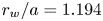$r_w/a = 1.194$ for the sharp boundary one. A variation in the rotation frequency results in a modification of the wall position for marginal stability. 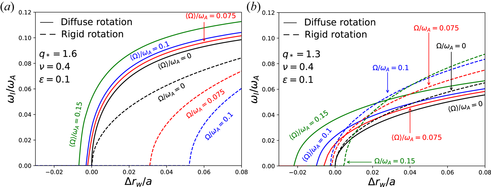Here, ${\rm \Delta} r_w/a$ measures this variation with respect to the wall position for marginal stability in the absence of flow. Figure 6(a) shows the results of these calculations for several rotation frequencies at a significant fraction of the Alfvén frequency. This figure illustrates that in order to suppress the external kink modes driven by flow shear it is necessary to displace the wall towards the plasma edge. The opposite behaviour is experienced in the case with rigid rotation. Nevertheless, for plasmas with the same average kinetic energy, the ${\rm \Delta} r_w/a$ modifications in the rigid rotation model are significantly larger than those in the diffuse scenario. This difference is (partly) attributed to the fact that in the sharp-boundary model, rotation produces an enhancement on the value of $\beta$ that enters in the boundary conditions. Essentially, the form for the equilibrium pressure profile $p(R) = p_o \exp [(R^2/R_o^2-1)M^2/2]$, is responsible for $\beta$-enhancement by a $(1+ M^2/2)$ factor. In contrast, $\varOmega (\varPsi)$ and $p(\varPsi)$ are not as tightly coupled in the diffuse model (although the constraints given by (2.20), (2.21), (2.27) and (2.28) should be satisfied). In order to accentuate the destabilizing effect of flow shear, which scales as ${\sim } 1/q_*^2$ ((2.13), (6.8), (A 4) and (A 5)), we consider a configuration with a lower value for the kink-safety factor next: $q_* = 1.3$. Starting at $\nu = 0.4$, and travelling along the $q_* = 1.3$ curve for the sharp-boundary model, an increase in $\beta$ pushes the wall position $r_w/a$ towards the plasma (figure 5). Accordingly, figure 6(b) illustrates the destabilizing influence of rigid rotation for $\varOmega /\omega _A = 0.075$ and $\varOmega /\omega _A =0.1$. At even higher rotation values (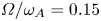$\varOmega /\omega _A = 0.15$), rigid flow is stabilizing. Contrary to figure 6(a), in figure 6(b) it is observed that the ${\rm \Delta} r_w/a$ modifications due to flow shear are of comparable order, and in fact larger, than those produced when the plasma rotates as a solid body.

Figure 6.

Comparison of growth rates of the $n = 1$ mode for plasmas with diffuse and rigid angular toroidal rotations. The comparison is performed at varying rotating frequencies of a significant fraction of the Alfvén frequency. Here, $\langle \varOmega (\varPsi) \rangle$ represents the average toroidal rotation over the plasma volume. Walls are assumed to be ideal, $\nu = 0.4$, $\epsilon = 0.1$ and the kink-safety factor is equal to (a) $q_*=1.6$ and (b) $q_*=1.3$. Here, ${\rm \Delta} r_w/a$ represents the displacement of the wall position for marginal stability in the presence of flow with respect to its position in the absence of it. Positions for marginal stability for static plasmas are given in figure 5. For case (a), $q_*=1.6$, the positions of marginal stability for the diffuse and the rigid rotation scenario are 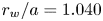$r_w/a = 1.040$ and $r_w/a = 1.194$, respectively. For case (b), $q_*=1.3$, these positions are 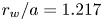$r_w/a = 1.217$ and 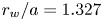$r_w/a = 1.327$, in the same order. In panel (b), the ${\rm \Delta} r_w/a$ modifications due to flow shear are larger than the ones due to rigid rotation; the opposite occurs in panel (a).

The comparison of the IPKM growth rates for plasmas with diffuse and rigid angular toroidal rotations in figure 6 are only qualitative. The stability of configurations where it is possible to control the level of flow shear, and where toroidal effects are retained, are probably better suited to be studied employing full numerical implementations (Chapman et al. Reference Chapman, Brown, Kemp and Walkden2012), but at the expense of capturing centrifugal and Coriolis effects as well. In this work, we have evaluated the effect of a high-$\beta$ flow shear drive while ordering out other velocity dependent contributions.

10. Summary and discussion

We have studied the linear stability of external $n=1$ modes for a tokamak plasma with a diffuse toroidal velocity profile and positive average finite magnetic shear. The effects of ideal and resistive walls are also considered. We have illustrated the stabilizing influence of the magnetic shear and the destabilizing nature of a global flow shear drive.

The stability analysis has been built upon a closed-form analytical equilibrium for a circular cross-section that is accurate to leading order in the inverse aspect ratio. In consequence, this ordering has been inherited at the stability level. Poloidal coupling is disregarded across the plasma column but is retained at the plasma–vacuum transition. Resonances enter in the stability analysis as if the configuration were cylindrical. Internal resonances are out of the scope of the present work and are avoided by selecting appropriate equilibrium parameters. Toroidal effects do enter into the stability picture; most notably, the flow shear drive for instabilities (6.8) is a high-$\beta$ toroidal effect. It has been determined that this effect is larger than centrifugal and Coriolis contributions provided that $\nu \gg \epsilon$. We perform a qualitative comparison of our model against a sharp-boundary scenario with a rigid angular toroidal frequency, which is based upon Betti (Reference Betti1998). Despite the fact that there are scenarios in which the destabilizing influence of flow shear is small as compared with the stability modifications in the presence of rigid rotation (figure 6a), figure 6(b) reveals that the (ideal) wall position for marginal stability might experience variations (${\rm \Delta} r_w/a$) of the same order of magnitude due to the destabilizing influence of a global flow shear drive, as in the case with rigid rotation.

The stability eigenvalue problem has been solved by implementing a multidimensional shooting method for the coupled poloidal harmonics. For static plasmas with no magnetic shear the eigenmode equation admits a trivial solution (8.2). This leads to a dispersion relation that is solvable with standard root finding methods. Eigenvalue/eigenvector pairs computed in this simple scenario function as robust initial guesses for the shooting method in situations with finite magnetic shear, toroidal velocity and resistive walls. The numerical implementation shoots from a position near the origin $(r = 0)$ ‘pointing towards’ the plasma–vacuum transition. Unfortunately, due to the fact that the equilibrium introduced in López & Guazzotto (Reference López and Guazzotto2017) possesses a singularity at the origin, the flow shear drive introduces this unphysical singularity at the eigenmode equation level. This issue has been addressed by constructing an alternative representation for the equilibrium that is regular on the complete plasma domain (appendix A).