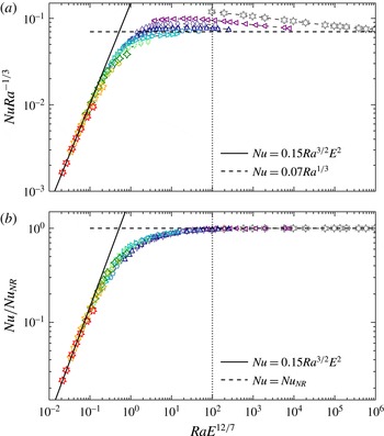
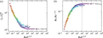
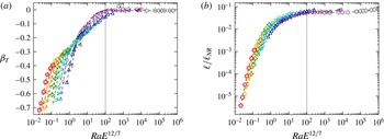
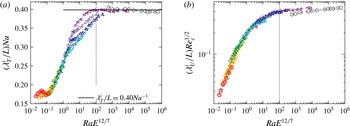
1 Introduction
Convection-driven flows under the influence of rotation are a ubiquitous physical phenomenon in the fluid interiors of natural objects. The liquid iron core of terrestrial planets, the envelopes of gas giants or the convective regions of rapidly rotating cool stars harbour highly turbulent convective flows strongly constrained by the dominant role of the Coriolis force. Rayleigh–Bénard convection (hereafter RBC) is a classical framework to examine the influence of rotation on turbulent convection. In its canonical form, rotating RBC consists of a planar fluid layer confined between two horizontal rigid plates separated from a distance
 $L$
, rotating about the vertical axis with a constant rotation rate
 $\unicode[STIX]{x1D6FA}$
. In this configuration, convective motions are driven by a fixed imposed temperature contrast
 $\unicode[STIX]{x0394}T$
between the two plates. The dynamics is then controlled by three dimensionless numbers, namely the Rayleigh number
 $Ra=\unicode[STIX]{x1D6FC}_{T}gL^{3}\unicode[STIX]{x0394}T/\unicode[STIX]{x1D708}\unicode[STIX]{x1D705}$
, the Ekman number
 $E=\unicode[STIX]{x1D708}/\unicode[STIX]{x1D6FA}L^{2}$
and the Prandtl number
 $Pr=\unicode[STIX]{x1D708}/\unicode[STIX]{x1D705}$
, where
 $\unicode[STIX]{x1D708}$
and
 $\unicode[STIX]{x1D705}$
are the viscous and thermal diffusivities,
 $\unicode[STIX]{x1D6FC}_{T}$
is the thermal expansivity and
 $g$
is the gravity. A combination of these parameters, named the convective Rossby number
 $Ro_{c}=Ra^{1/2}E/Pr^{1/2}$
, is frequently employed as a reasonable proxy of the ratio between the global-scale buoyancy and Coriolis forces (Gilman Reference Gilman1977). The key issue in RBC is to explore the efficiency of the heat and momentum transports across the layer. Important quantities in this regard are the Reynolds number
 $Re$
and the dimensionless heat transport, defined by the Nusselt number
 $Nu={\mathcal{Q}}L/\unicode[STIX]{x1D70C}c_{p}\unicode[STIX]{x1D705}\unicode[STIX]{x0394}T$
, where
 ${\mathcal{Q}}$
is the total heat flux,
 $\unicode[STIX]{x1D70C}$
is the density and
 $c_{p}$
the heat capacity. The Nusselt number is the most widely studied diagnostic since it can be easily measured experimentally and numerically and then compared to numerical and theoretical predictions. The understanding of the scaling dependence of
 $Nu$
upon the control parameters
 $Ra$
,
 $E$
and
 $Pr$
is of paramount importance to identify the different regimes and to possibly extrapolate the scaling behaviours to natural objects.
Rotational constraints delay the onset of convection and the critical Rayleigh number increases with increasing rotation rate as
 $Ra_{c}\sim E^{-4/3}$
when
 $E\rightarrow 0$
(Chandrasekhar Reference Chandrasekhar1961). The convective pattern takes the form of elongated Taylor columns which have a typical horizontal size
 $\ell \sim E^{1/3}L$
and are aligned with the rotation axis. Beyond
 $Ra_{c}$
, the heat transport rises much more rapidly than for non-rotating convection (e.g. Rossby Reference Rossby1969; Boubnov & Golitsyn Reference Boubnov and Golitsyn1990). Hence, if the Rayleigh number is continuously increased far beyond
 $Ra_{c}$
at a given Ekman number, the heat transfer properties will eventually transition to a state where rotational effects become secondary. In this weakly rotating regime with
 $Ro_{c}\gg 1$
, the scaling properties become essentially reminiscent to non-rotating RBC (e.g. Liu & Ecke Reference Liu and Ecke1997; Zhong et al.
Reference Zhong, Stevens, Clercx, Verzicco, Lohse and Ahlers2009). The heat transport scaling is then expected to become independent of the Ekman number and to approach the scalings obtained in classical RBC, i.e.
 $Nu\sim Ra^{\unicode[STIX]{x1D708}_{eff}}$
, with
 $0.27\leqslant \unicode[STIX]{x1D708}_{eff}\leqslant 1/3$
for
 $10^{5}\leqslant Ra\leqslant 10^{12}$
(e.g. Grossmann & Lohse Reference Grossmann and Lohse2000; Funfschilling et al.
Reference Funfschilling, Brown, Nikolaenko and Ahlers2005; Ahlers, Grossmann & Lohse Reference Ahlers, Grossmann and Lohse2009; Chillà & Schumacher Reference Chillà and Schumacher2012).
A turbulent regime of rotating convection is expected when both
 $Ro_{c}\ll 1$
and
 $Re\gg 1$
. This implies large supercriticalities in combination with low Ekman numbers to ensure that the rotational constraints are not lost. This parameter range is therefore particularly difficult to explore with current-day laboratory experiments and numerical simulations (see Aurnou et al.
Reference Aurnou, Calkins, Cheng, Julien, King, Nieves, Soderlund and Stellmach2015). In the following, we make the assumption that the heat transport scaling can be written as
 $$\begin{eqnarray}Nu\sim Ra^{\unicode[STIX]{x1D6FC}}E^{\unicode[STIX]{x1D6FD}}Pr^{\unicode[STIX]{x1D6FE}}\end{eqnarray}$$
in this regime. In general however, the values of the exponents
 $\unicode[STIX]{x1D6FC}$
,
 $\unicode[STIX]{x1D6FD}$
and
 $\unicode[STIX]{x1D6FE}$
might well continuously vary with
 $Ra$
, similarly to classical RBC (Grossmann & Lohse Reference Grossmann and Lohse2000). In contrast to non-rotating convection, where the heat transport is controlled by diffusive processes in the thermal boundary layers, a dominant fraction of the temperature difference is accommodated in the fluid bulk when
 $Ro_{c}\ll 1$
(e.g. Boubnov & Golitsyn Reference Boubnov and Golitsyn1990; Schmitz & Tilgner Reference Schmitz and Tilgner2009; Kunnen, Geurts & Clercx Reference Kunnen, Geurts and Clercx2010; Julien et al.
Reference Julien, Rubio, Grooms and Knobloch2012b
; King, Stellmach & Buffett Reference King, Stellmach and Buffett2013). We can therefore hypothesise that the heat transport is controlled by the fluid bulk rather than by the thermal boundary layers that play an important role in the weakly rotating limit. Because the viscous dissipation is rather weak in the fluid interior, we make the assumption that
 $Nu$
will thus become independent of the diffusivities
 $\unicode[STIX]{x1D708}$
and
 $\unicode[STIX]{x1D705}$
in the asymptotic limit of rapidly rotating convection (Gillet & Jones Reference Gillet and Jones2006; Jones Reference Jones and Schubert2015). From the definition of
 $Ra$
,
 $E$
,
 $Pr$
and
 $Nu$
, this requirement yields the following combination of the scaling exponents
 $$\begin{eqnarray}-\unicode[STIX]{x1D6FC}+\unicode[STIX]{x1D6FD}+\unicode[STIX]{x1D6FE}=0,\quad \unicode[STIX]{x1D6FC}+\unicode[STIX]{x1D6FE}=1.\end{eqnarray}$$
In the limit of non-rotating convection, the dependence on
 $E$
vanishes (i.e.
 $\unicode[STIX]{x1D6FD}=0$
) and the previous relationship between the scaling exponents relating
 $\unicode[STIX]{x1D6FC}$
and
 $\unicode[STIX]{x1D6FE}$
yields the so-called ultimate regime of classical RBC
 $Nu\sim Ra^{1/2}Pr^{1/2}$
(Kraichnan Reference Kraichnan1962). Numerical models of rotating convection by King, Stellmach & Aurnou (Reference King, Stellmach and Aurnou2012) further indicate that the heat flux might only depend on the supercriticality
 $Ra/Ra_{c}$
when
 $Ro_{c}\ll 1$
(see also Julien et al.
Reference Julien, Knobloch, Rubio and Vasil2012a
; Stellmach et al.
Reference Stellmach, Lischper, Julien, Vasil, Cheng, Ribeiro, King and Aurnou2014). This second hypothesis yields
 $\unicode[STIX]{x1D6FD}=4\unicode[STIX]{x1D6FC}/3$
when
 $E\rightarrow 0$
and allows us to derive the following diffusivity-free scaling for rotating convection
 $$\begin{eqnarray}Nu\sim Ra^{3/2}E^{2}Pr^{-1/2}.\end{eqnarray}$$
Gillet & Jones (Reference Gillet and Jones2006) derive the same equation under the hypothesis that a triple force balance between Coriolis force, inertia and buoyancy controls the asymptotic regime of rapidly rotating turbulent convection (see also Stevenson Reference Stevenson1979; Barker, Dempsey & Lithwick Reference Barker, Dempsey and Lithwick2014). The analysis carried out by Julien et al. (Reference Julien, Knobloch, Rubio and Vasil2012a
) leads to the same inviscid scaling in the framework of asymptotically reduced equations expected to hold when
 $E\rightarrow 0$
. The evidence for such a low-
 $Ro_{c}$
scaling law is however strongly debated. Specifically, King et al. (Reference King, Stellmach and Aurnou2012) suggest a much steeper heat transport scaling
 $Nu\sim Ra^{3}E^{4}$
for
 $E=O(10^{-5})$
and
 $Ro_{c}=O(0.1)$
, based on laboratory experiments in water complemented by numerical simulations of rotating convection with rigid mechanical boundaries in Cartesian coordinates (see also King et al.
Reference King, Stellmach and Buffett2013). Similar numerical models by Schmitz & Tilgner (Reference Schmitz and Tilgner2009) that instead employ stress-free boundaries rather found
 $Nu\sim (Ra\,E^{4/3})^{1.22}$
for a comparable parameter range. This discrepancy implies that the viscous boundary layers might still have a direct influence on the heat transport even at low
 $E$
. The recent comparative study by Stellmach et al. (Reference Stellmach, Lischper, Julien, Vasil, Cheng, Ribeiro, King and Aurnou2014) for rigid and stress-free numerical models at lower Ekman numbers
 $E=O(10^{-7})$
indeed reveals an active role of the Ekman boundary layers (see also Kunnen et al.
Reference Kunnen, Ostilla-Mónico, van der Poel, Verzicco and Lohse2016; Plumley et al.
Reference Plumley, Julien, Marti and Stellmach2016). While the stress-free models gradually approach the diffusivity-free scaling (1.3) (see also Barker et al.
Reference Barker, Dempsey and Lithwick2014), the Ekman pumping in the cases with rigid boundaries leads to increasing scaling exponents when
 $E$
is decreased towards geophysical values (Cheng et al.
Reference Cheng, Stellmach, Ribeiro, Grannan, King and Aurnou2015; Julien et al.
Reference Julien, Aurnou, Calkins, Knobloch, Marti, Stellmach and Vasil2016). This prominent role of the boundary layers therefore questions the relevance of the inviscid scaling (1.3) for rigid boundaries.
Although the spherical geometry is more natural for studying rotating convection in astrophysical and geophysical objects, the majority of the rotating RBC laboratory experiments developed over the past three decades have been carried out in planar and cylindrical cells, in which the rotation axis and the gravity are aligned. The Cartesian geometry also allows the computation of efficient local direct numerical simulations that operate at low Ekman numbers (e.g. Kunnen et al.
Reference Kunnen, Geurts and Clercx2010; Ecke & Niemela Reference Ecke and Niemela2014; Horn & Shishkina Reference Horn and Shishkina2015). Hence, the fruitful interplay between numerical and laboratory experiments in planar or cylindrical geometries enabled a complementary coverage of the parameter space in the low-
 $Ro_{c}$
regime (e.g. Aurnou Reference Aurnou2007; Stellmach et al.
Reference Stellmach, Lischper, Julien, Vasil, Cheng, Ribeiro, King and Aurnou2014; Aurnou et al.
Reference Aurnou, Calkins, Cheng, Julien, King, Nieves, Soderlund and Stellmach2015; Cheng et al.
Reference Cheng, Stellmach, Ribeiro, Grannan, King and Aurnou2015). However, it remains unclear whether the planar RBC results can be directly applied to rotating convection in spherical geometry. Two specific features of thermal convection in rotating spherical shells are indeed expected to yield significant dynamical differences with the planar or cylindrical RBC set-ups: (i) in most of the fluid volume of spherical shells, gravity is inclined with respect to the rotation axis; (ii) due to both curvature and radial variations of the gravitational acceleration, spherical RBC features a significant asymmetry between the hot and the cold bounding surfaces (e.g. Bercovici et al.
Reference Bercovici, Schubert, Glatzmaier and Zebib1989; Jarvis Reference Jarvis1993; Gastine, Wicht & Aurnou Reference Gastine, Wicht and Aurnou2015).
Besides the micro-gravity experiments that operate at relatively large Ekman numbers due to their moderate sizes (
 $E=O(10^{-3})$
, see Hart, Glatzmaier & Toomre Reference Hart, Glatzmaier and Toomre1986; Egbers et al.
Reference Egbers, Beyer, Bonhage, Hollerbach and Beltrame2003), most of the laboratory investigations of spherical rotating RBC make use of the centrifugal force as a surrogate for the radial gravitational acceleration (Busse & Carrigan Reference Busse and Carrigan1974; Cardin & Olson Reference Cardin and Olson1994; Sumita & Olson Reference Sumita and Olson2003; Shew & Lathrop Reference Shew and Lathrop2005). The combined influence of the laboratory gravity and the centrifugal acceleration of the rotating vessel indeed allows generation of surfaces of gravity potential close to the spherical surfaces in the lower hemisphere of the spherical shell (see for a review Cardin & Olson Reference Cardin, Olson and Schubert2015). This technique was first employed to explore the onset of convection in rotating spherical RBC (Cordero & Busse Reference Cordero and Busse1992). Sumita & Olson (Reference Sumita and Olson2003) studied the scaling behaviours of the heat transport for a relatively low Ekman number (
 $E\simeq 5\times 10^{-6}$
) but with a strong convective forcing (
 $Ra\geqslant 200\,Ra_{c}$
). In this parameter range, they obtained
 $Nu\sim Ra^{0.41}$
, a scaling exponent that is hardly steeper than non-rotating RBC and therefore suggests that the Coriolis force only plays a minor role on the heat transfer.
Numerical simulations of three-dimensional convection in spherical shells have been developed since the late 1970s as a complementary approach to the laboratory experiments (e.g. Gilman Reference Gilman1977; Tilgner & Busse Reference Tilgner and Busse1997; Christensen Reference Christensen2002). Christensen & Aubert (Reference Christensen and Aubert2006), later complemented by King et al. (Reference King, Soderlund, Christensen, Wicht and Aurnou2010), conducted a systematic parameter study of the scaling properties of convective dynamo models with rigid boundaries and reported the scaling
 $Nu\sim Ra^{6/5}E^{8/5}$
for
 $E=O(10^{-5})$
. These studies were however carried out in the presence of a self-sustained magnetic field that can possibly impinge on the heat transport. More recently, Yadav et al. (Reference Yadav, Gastine, Christensen, Duarte and Reiners2016) studied the influence of both the presence of a magnetic field and the nature of the mechanical boundary condition on the heat transfer in spherical RBC. Magnetic and non-magnetic models were found to exhibit similar heat transfer scaling behaviours possibly because of the parameter space limitation to
 $E=O(10^{-5})$
(see also Soderlund, King & Aurnou Reference Soderlund, King and Aurnou2012; Garcia, Sánchez & Net Reference Garcia, Sánchez and Net2014). Furthermore, these authors did not observe the steep increase of the
 $Ra$
-scaling exponent beyond
 $3/2$
reported in the Cartesian calculations (e.g. King et al.
Reference King, Stellmach and Aurnou2012) when rigid boundaries were employed. Since the heat transport in spherical shells is dominated by the equatorial regions where the gravity is nearly perpendicular to the rotation axis (Tilgner & Busse Reference Tilgner and Busse1997; Yadav et al.
Reference Yadav, Gastine, Christensen, Duarte and Reiners2016), it is not entirely surprising that the scaling properties differ from the Cartesian models that would best represent the high-latitude dynamics of a spherical shell.
While
 $Nu$
is a ubiquitous diagnostic quantity studied in both laboratory experiments and numerical models; numerical calculations also enable the computation of additional diagnostics that can provide direct insights on the dynamical regimes. In that regard, the scaling analysis of the convective flow speed
 $Re$
and the typical length scale
 $\ell$
can be used to disentangle the underlying force balance in rotating RBC (Aubert et al.
Reference Aubert, Brito, Nataf, Cardin and Masson2001; King & Buffett Reference King and Buffett2013). Two theoretical scalings for
 $Re$
and
 $\ell$
have been put forward. The first one, frequently called the inertial scaling of rotating convection, hypothesises a triple force balance between Coriolis, inertia and Archimedean forces (CIA scaling, see Stevenson Reference Stevenson1979; Cardin & Olson Reference Cardin and Olson1994; Aubert et al.
Reference Aubert, Brito, Nataf, Cardin and Masson2001; Barker et al.
Reference Barker, Dempsey and Lithwick2014), while the second rather relies on a triple balance between viscosity, Archimedean and Coriolis forces (VAC scaling, see King et al.
Reference King, Stellmach and Buffett2013). These two concurrent theories however lead to scaling exponents for
 $Re(Ra,E,Pr)$
close to each other. Using the numerical dataset by Christensen & Aubert (Reference Christensen and Aubert2006), King & Buffett (Reference King and Buffett2013) even demonstrated that these limited data can support both
 $Re$
-scalings at the same statistical confidence level. This study indicates a sizeable role played by viscosity in rotating RBC models with
 $E\geqslant 10^{-5}$
. To decrease the numerical cost of direct three-dimensional calculations, the quasi-geostrophic approximation of spherical convection (hereafter QG, see Busse & Or Reference Busse and Or1986; Cardin & Olson Reference Cardin and Olson1994) has been developed. In the limit of
 $E\rightarrow 0$
and
 $Ro_{c}\ll 1$
, convection is strongly constrained by rotation and can be approximated by a quasi-two-dimensional flow, which allows us to decrease the Ekman number to
 $E=O(10^{-7})$
(Aubert, Gillet & Cardin Reference Aubert, Gillet and Cardin2003; Gillet & Jones Reference Gillet and Jones2006; Guervilly Reference Guervilly2010). However, the scaling analyses carried out by Gillet & Jones (Reference Gillet and Jones2006) and Guervilly (Reference Guervilly2010) did not show any clear evidence of convergence towards the diffusivity-free scalings for both
 $Nu$
and
 $Re$
, even when
 $E\lesssim 10^{-6}$
. Furthermore, the lack of a direct one-to-one comparison between the QG results and the fully three-dimensional computations makes the interpretation of these results difficult. Hence, the determination of an accurate scaling law for both
 $Re$
and
 $\ell$
in rapidly rotating spherical RBC forms one of the main goals of this work.
The aims of this study are twofold: (i) to determine the boundaries of the different physical regimes of rapidly rotating convection in spherical shells by means of three-dimensional numerical simulations; (ii) to establish the scaling behaviours of both the local (length scale, boundary layers) and the global (
 $Nu$
and
 $Re$
) properties that hold within each of these different regimes. We conduct a systematic parameter study varying the Ekman number within the range
 $3\times 10^{-7}\leqslant E\leqslant 10^{-1}$
and the Rayleigh number within the range
 $10^{3}\lesssim Ra\lesssim 2\times 10^{10}$
for a unity Prandtl number spherical shell of radius ratio
 $r_{i}/r_{o}=0.6$
. To do so, we construct a dataset of 227 rotating simulations that complement our previous non-rotating calculations (Gastine et al.
Reference Gastine, Wicht and Aurnou2015). Recent improvements of pseudo-spectral numerical codes (Schaeffer Reference Schaeffer2013) enabled us to decrease the Ekman number to values comparable to these used in present-day local Cartesian calculations. Our dataset allows us to determine the regime boundaries for rotating convection and to check the validity of the diffusivity-free scaling (1.3) in the low-
 $E$
regime. We examine the scaling behaviours of seven different diagnostics:
 $Nu$
and
 $Re$
, the viscous dissipation rate, the typical flow length scale, the interior temperature gradient and the viscous and the thermal boundary layer thicknesses.
In § 2, we introduce the hydrodynamical model and the various diagnostic quantities of interest. The numerical results are presented in § 3. We conclude with a summary of our findings in § 4.
2 Formulation of the hydrodynamical problem
2.1 Governing equations
We consider rotating convection of a Boussinesq fluid confined in a spherical shell that rotates at a constant frequency
 $\unicode[STIX]{x1D6FA}$
about the
 $z$
axis. Convective motions are driven by a fixed temperature contrast
 $\unicode[STIX]{x0394}T=T_{i}-T_{o}$
between the inner radius
 $r_{i}$
and the outer radius
 $r_{o}$
. The boundaries are impermeable, no slip and held at constant temperatures. We adopt a dimensionless formulation of the Navier–Stokes equations using the shell thickness
 $L=r_{o}-r_{i}$
as the reference length scale and the viscous diffusion time
 $L^{2}/\unicode[STIX]{x1D708}$
as the reference time scale. The temperature contrast
 $\unicode[STIX]{x0394}T$
defines the temperature scale and gravity is non-dimensionalised using its reference value at the outer boundary
 $g_{o}$
. The dimensionless equations that govern convective motions for the velocity
 $\boldsymbol{u}$
, the pressure
 $p$
and the temperature
 $T$
are then expressed by
 $$\begin{eqnarray}\displaystyle & \displaystyle \unicode[STIX]{x1D735}\boldsymbol{\cdot }\tilde{\boldsymbol{u}}=0, & \displaystyle\end{eqnarray}$$
 $$\begin{eqnarray}\displaystyle & \displaystyle \frac{\unicode[STIX]{x2202}\tilde{\boldsymbol{u}}}{\unicode[STIX]{x2202}t}+\tilde{\boldsymbol{u}}\boldsymbol{\cdot }\unicode[STIX]{x1D735}\tilde{\boldsymbol{u}}+{\displaystyle \frac{2}{E}}\,\boldsymbol{e}_{z}\times \tilde{\boldsymbol{u}}=-\unicode[STIX]{x1D735}\tilde{p}+\frac{Ra}{Pr}\,\tilde{g}\,\tilde{T}\,\boldsymbol{e}_{r}+\unicode[STIX]{x1D6AB}\tilde{\boldsymbol{u}}, & \displaystyle\end{eqnarray}$$
 $$\begin{eqnarray}\displaystyle & \displaystyle \frac{\unicode[STIX]{x2202}\tilde{T}}{\unicode[STIX]{x2202}t}+\tilde{\boldsymbol{u}}\boldsymbol{\cdot }\unicode[STIX]{x1D735}\tilde{T}=\frac{1}{Pr}\unicode[STIX]{x0394}\tilde{T}, & \displaystyle\end{eqnarray}$$
where the tildes designate the dimensionless variables. The units vectors in the radial and vertical directions are denoted by
 $\boldsymbol{e}_{r}$
and
 $\boldsymbol{e}_{z}$
, respectively. We make the assumption of a centrally condensed mass which yields a dimensionless gravity profile of the form
 $\tilde{g}=(r_{o}/r)^{2}$
. This particular choice is motivated by the exact analytical relation between the buoyancy power and the so-called flux-based Rayleigh number when
 $\tilde{g}\sim 1/r^{2}$
(see below and Gastine et al.
Reference Gastine, Wicht and Aurnou2015). This enables us to conduct an exact analysis of the viscous dissipation rate and to directly compare our numerical models with our previous calculations of non-rotating convection which employed the same gravity profile.
The dimensionless equations (2.1)–(2.3) are governed by the Ekman number
 $E$
, the Rayleigh number
 $Ra$
, the Prandtl number
 $Pr$
and the radius ratio of the spherical shell
 $\unicode[STIX]{x1D702}$
defined by
 $$\begin{eqnarray}E=\frac{\unicode[STIX]{x1D708}}{\unicode[STIX]{x1D6FA}L^{2}},\quad Ra=\frac{\unicode[STIX]{x1D6FC}_{T}g_{o}\unicode[STIX]{x0394}TL^{3}}{\unicode[STIX]{x1D708}\unicode[STIX]{x1D705}},\quad Pr=\frac{\unicode[STIX]{x1D708}}{\unicode[STIX]{x1D705}},\quad \unicode[STIX]{x1D702}=\frac{r_{i}}{r_{o}},\end{eqnarray}$$
where
 $\unicode[STIX]{x1D6FC}_{T}$
is the thermal expansion coefficient,
 $\unicode[STIX]{x1D708}$
is the kinematic viscosity and
 $\unicode[STIX]{x1D705}$
is the thermal diffusivity. In the following, we will also consider the convective Rossby number,
 $Ro_{c}$
, expressed by
 $$\begin{eqnarray}Ro_{c}=\sqrt{\frac{\unicode[STIX]{x1D6FC}_{T}g_{o}\unicode[STIX]{x0394}T}{\unicode[STIX]{x1D6FA}^{2}L}}=\frac{Ra^{1/2}E}{Pr^{1/2}},\end{eqnarray}$$
which provides a good proxy of the relative importance of buoyancy forcing and Coriolis force in rotating convection (e.g. Gilman Reference Gilman1977).
2.2 Numerical technique
The numerical simulations carried out in this study have been computed using the open-source magnetohydrodynamics code MagIC (Wicht Reference Wicht2002; Gastine et al.
Reference Gastine, Wicht, Barik, Putigny and Duarte2016). (Available at http://www.github.com/magic-sph/magic.) MagIC has been validated via several benchmark tests for convection and dynamo action in a spherical shell geometry (Christensen et al.
Reference Christensen, Aubert, Cardin, Dormy, Gibbons, Glatzmaier, Grote, Honkura, Jones and Kono2001; Jones et al.
Reference Jones, Boronski, Brun, Glatzmaier, Gastine, Miesch and Wicht2011). To solve the system of equations (2.1)–(2.3) in spherical coordinates
 $(r,\unicode[STIX]{x1D703},\unicode[STIX]{x1D719})$
, the velocity field is decomposed into a poloidal and a toroidal contribution
 $$\begin{eqnarray}\tilde{\boldsymbol{u}}=\unicode[STIX]{x1D735}\times \left(\unicode[STIX]{x1D735}\times \tilde{W}\boldsymbol{e}_{r}\right)+\unicode[STIX]{x1D735}\times \tilde{Z}\boldsymbol{e}_{r},\end{eqnarray}$$
where
 $\tilde{W}$
and
 $\tilde{Z}$
are the poloidal and toroidal potentials. The dimensionless unknowns
 $\tilde{W}$
,
 $\tilde{Z}$
,
 $\tilde{p}$
and
 $\tilde{T}$
are expanded in spherical harmonic functions up to degree
 $l_{max}$
in the colatitude
 $\unicode[STIX]{x1D703}$
and longitude
 $\unicode[STIX]{x1D719}$
and in Chebyshev polynomials up to degree
 $N_{r}$
in the radial direction. The equations are time advanced using an explicit second-order Adams–Bashforth scheme for the Coriolis acceleration and the nonlinear terms and an implicit Crank–Nicolson algorithm for the remaining linear terms. The explicit treatment of the Coriolis force implies that the dimensionless time step size is limited to a fraction of the rotation period. For a comprehensive description of the numerical method and the associated spectral transforms, the reader is referred to Gilman & Glatzmaier (Reference Gilman and Glatzmaier1981), Tilgner & Busse (Reference Tilgner and Busse1997) and Christensen & Wicht (Reference Christensen, Wicht and Schubert2015). For the most demanding calculations, MagIC uses the open-source library SHTns to speed up the spherical harmonic transforms (Schaeffer Reference Schaeffer2013). (Available at https://bitbucket.org/nschaeff/shtns.)
2.3 Diagnostics
We introduce in the following several diagnostic properties to quantify the impact of the different control parameters on the flow and temperature properties. We adopt several notations regarding averaging procedures. Overbars
 $\overline{\cdots \,}$
correspond to temporal averaging, angular brackets
 $\langle \,\cdots \,\rangle$
to spatial averaging over the entire spherical shell volume and
 $\langle \,\cdots \,\rangle _{s}$
to an average over a spherical surface
 $$\begin{eqnarray}\overline{f}={\displaystyle \frac{1}{\unicode[STIX]{x1D70F}}}\int _{t_{0}}^{t_{0}+\unicode[STIX]{x1D70F}}f\,\text{d}t,\quad \left\langle f\right\rangle =\frac{1}{V}\int _{V}f(r,\unicode[STIX]{x1D703},\unicode[STIX]{x1D719})\,\text{d}V,\quad \left\langle f\right\rangle _{s}=\frac{1}{4\unicode[STIX]{x03C0}}\int _{0}^{\unicode[STIX]{x03C0}}\int _{0}^{2\unicode[STIX]{x03C0}}f(r,\unicode[STIX]{x1D703},\unicode[STIX]{x1D719})\sin \unicode[STIX]{x1D703}\,\text{d}\unicode[STIX]{x1D703}\,\text{d}\unicode[STIX]{x1D719},\end{eqnarray}$$
where
 $V$
is the spherical shell volume and
 $\unicode[STIX]{x1D70F}$
is the time averaging interval.
For the sake of clarity, we introduce the notation
 $\unicode[STIX]{x1D717}$
to define the time and horizontally averaged radial dimensionless temperature profile
 $$\begin{eqnarray}\unicode[STIX]{x1D717}(r)=\overline{\langle \tilde{T}\rangle _{s}}.\end{eqnarray}$$
The heat transport is characterised by the Nusselt number
 $Nu$
, the ratio of the total heat flux to the heat carried by conduction
 $$\begin{eqnarray}Nu=\frac{\unicode[STIX]{x1D702}\,{\mathcal{Q}}\,L}{\unicode[STIX]{x1D70C}c_{p}\unicode[STIX]{x1D705}\unicode[STIX]{x0394}T}=\frac{\displaystyle \left.\frac{\text{d}\unicode[STIX]{x1D717}}{\text{d}r}\right|_{r=r_{o}}}{\displaystyle \left.\frac{\text{d}\tilde{T}_{c}}{\text{d}r}\right|_{r=r_{o}}}=\frac{\displaystyle \left.\frac{\text{d}\unicode[STIX]{x1D717}}{\text{d}r}\right|_{r=r_{i}}}{\displaystyle \left.\frac{\text{d}\tilde{T}_{c}}{\text{d}r}\right|_{r=r_{i}}},\end{eqnarray}$$
where
 ${\mathcal{Q}}$
is the heat flux,
 $c_{p}$
is the heat capacity and
 $\tilde{T}_{c}$
is the dimensionless conductive temperature profile, solution of
 $$\begin{eqnarray}\frac{\text{d}}{\text{d}r}\left(r^{2}\frac{\text{d}\tilde{T}_{c}}{\text{d}r}\right)=0,\quad \tilde{T}_{c}(r_{i})=1,\quad \tilde{T}_{c}(r_{o})=0.\end{eqnarray}$$
The dimensionless kinetic energy
 $\tilde{E}_{k}$
is defined by
 $$\begin{eqnarray}\tilde{E}_{k}={\displaystyle \frac{1}{2}}\overline{\langle \tilde{u} ^{2}\rangle }=\mathop{\sum }_{l=1}^{l_{max}}\mathop{\sum }_{m=0}^{l}{\mathcal{E}}_{l}^{m},\end{eqnarray}$$
where
 ${\mathcal{E}}_{l}^{m}$
is the dimensionless kinetic energy density at a spherical harmonic degree
 $l$
and order
 $m$
. In rotating spherical shells, the axisymmetric zonal flow can represent a significant fraction of the total kinetic energy (e.g. Christensen Reference Christensen2002; Gastine & Wicht Reference Gastine and Wicht2012; Yadav et al.
Reference Yadav, Gastine, Christensen, Duarte and Reiners2016). Since this flow does not directly contribute to the heat transfer, we decide to rather characterise the root-mean-square (r.m.s.) flow velocity by the time-averaged convective Reynolds number expressed by
 $$\begin{eqnarray}Re_{c}=\overline{\sqrt{2\mathop{\sum }_{l=1}^{l_{max}}\mathop{\sum }_{m=1}^{l}{\mathcal{E}}_{l}^{m}}},\end{eqnarray}$$
where the contribution from the axisymmetric flows (
 $m=0$
) has been excluded. The fluid bulk in rotating convection usually departs from the well-mixed convective interior obtained in classical RBC. Under the influence of rapid rotation, turbulent mixing is inhibited and strong interior temperature gradients can persist (e.g. Julien et al.
Reference Julien, Legg, McWilliams and Werne1996; King et al.
Reference King, Stellmach, Noir, Hansen and Aurnou2009; Stellmach et al.
Reference Stellmach, Lischper, Julien, Vasil, Cheng, Ribeiro, King and Aurnou2014). We denote the bulk temperature gradient at mid-shell by
 $$\begin{eqnarray}\unicode[STIX]{x1D6FD}_{T}=\left.\frac{\text{d}\unicode[STIX]{x1D717}}{\text{d}r}\right|_{r=r_{m}},\quad r_{m}=\frac{1+\unicode[STIX]{x1D702}}{2(1-\unicode[STIX]{x1D702})}.\end{eqnarray}$$
Following Christensen & Aubert (Reference Christensen and Aubert2006), the typical flow length scale is determined from the time-averaged kinetic energy spectrum
 $$\begin{eqnarray}\ell ^{-1}=\overline{\left(\frac{L\,\displaystyle \mathop{\sum }_{l=1}^{l_{max}}\mathop{\sum }_{m=0}^{l}l\,{\mathcal{E}}_{l}^{m}(t)}{\unicode[STIX]{x03C0}\,\displaystyle \mathop{\sum }_{l=1}^{l_{max}}\mathop{\sum }_{m=0}^{l}{\mathcal{E}}_{l}^{m}(t)}\right)}.\end{eqnarray}$$
Several different approaches have been considered to define the thermal boundary layer thickness
 $\unicode[STIX]{x1D706}_{T}$
. They either rely on the mean radial temperature profile
 $\unicode[STIX]{x1D717}(r)$
(e.g. Verzicco & Camussi Reference Verzicco and Camussi1999; Breuer et al.
Reference Breuer, Wessling, Schmalzl and Hansen2004; Liu & Ecke Reference Liu and Ecke2011) or on the r.m.s. of the temperature fluctuations (e.g. Julien et al.
Reference Julien, Rubio, Grooms and Knobloch2012b
; King et al.
Reference King, Stellmach and Buffett2013; Kunnen et al.
Reference Kunnen, Ostilla-Mónico, van der Poel, Verzicco and Lohse2016). For consistency with the definition adopted in our non-rotating calculations (Gastine et al.
Reference Gastine, Wicht and Aurnou2015),
 $\unicode[STIX]{x1D706}_{T}^{i}$
(
 $\unicode[STIX]{x1D706}_{T}^{o}$
) is defined here as the depth where the linear fit to the temperature profile near the inner (outer) boundary intersects the linear fit to the profile at mid-depth. The comparison of this boundary layer definition with the estimate coming from the location of the peaks of the r.m.s. of the temperature fluctuations for a few selected cases yield similar boundary layer thicknesses. The viscous boundary layer thicknesses are estimated following a similar slope-intersection method:
 $\unicode[STIX]{x1D706}_{U}^{i}$
(
 $\unicode[STIX]{x1D706}_{U}^{o}$
) is defined as the distance from the inner (outer) boundary where the linear fit to the horizontal velocity profile
 $u_{h}=\sqrt{u_{\unicode[STIX]{x1D703}}^{2}+u_{\unicode[STIX]{x1D719}}^{2}}$
near the inner (outer) boundary intersects the horizontal line passing through the maximum of
 $u_{h}$
(see also Breuer et al.
Reference Breuer, Wessling, Schmalzl and Hansen2004).
2.4 Parameter choice and resolution checks
We aim at studying the scaling behaviours of both the local (length scales, temperature gradient, boundary layers) and the global (Nusselt and Reynolds numbers) properties for each dynamical regimes of rotating convection in spherical shells. To achieve this goal, we build a dataset of 227 global spherical shell models that span the range
 $3\times 10^{-7}\leqslant E\leqslant 10^{-1}$
and
 $10^{3}<Ra<2\times 10^{10}$
. The radius ratio
 $\unicode[STIX]{x1D702}$
is kept fixed to
 $\unicode[STIX]{x1D702}=0.6$
and the Prandtl number to
 $Pr=1$
to limit the extension of the parameter space. This set-up also allows a direct comparison with our previous non-rotating models (Gastine et al.
Reference Gastine, Wicht and Aurnou2015). The numerical dataset constructed in this study thoroughly explores various dynamical regimes of rotating convection encompassing convection close to critical, turbulent quasi-geostrophic convection and weakly rotating convection. The summary table 2 given in appendix A contains the calculations of the main control and diagnostic quantities computed for each numerical simulation.
Particular attention must be paid to the numerical resolution requirements for global models of convection (Shishkina et al.
Reference Shishkina, Stevens, Grossmann and Lohse2010; King et al.
Reference King, Stellmach and Aurnou2012), since under-resolution can significantly degrade the accuracy of the obtained exponents when deriving asymptotic scaling laws (Amati et al.
Reference Amati, Koal, Massaioli, Sreenivasan and Verzicco2005). The comparison of the viscous and thermal dissipation rates with the time-averaged Nusselt number provides a robust way to validate the numerical resolutions employed in our models (e.g. Stevens, Verzicco & Lohse Reference Stevens, Verzicco and Lohse2010; Lakkaraju et al.
Reference Lakkaraju, Stevens, Verzicco, Grossmann, Prosperetti, Sun and Lohse2012). As demonstrated in our previous RBC calculations (Gastine et al.
Reference Gastine, Wicht and Aurnou2015), the choice of a centrally condensed mass (i.e.
 $\tilde{g}\sim 1/r^{2}$
) ensures the following analytical relations between the dimensionless viscous dissipation rate
 $\tilde{\unicode[STIX]{x1D716}}_{U}$
and the flux-based Rayleigh number defined by
 $Ra_{{\mathcal{Q}}}=Ra(Nu-1)$
:
 $$\begin{eqnarray}\tilde{\unicode[STIX]{x1D716}}_{U}=\overline{\left\langle (\unicode[STIX]{x1D735}\times \tilde{\boldsymbol{u}})^{2}\right\rangle }=\frac{3}{1+\unicode[STIX]{x1D702}+\unicode[STIX]{x1D702}^{2}}\,\frac{Ra_{{\mathcal{Q}}}}{Pr^{2}},\end{eqnarray}$$
and between the dimensionless thermal dissipation rate
 $\tilde{\unicode[STIX]{x1D716}}_{T}$
and the Nusselt number
 $$\begin{eqnarray}\tilde{\unicode[STIX]{x1D716}}_{T}=\overline{\left\langle (\unicode[STIX]{x1D735}\tilde{T})^{2}\right\rangle }=\frac{3\unicode[STIX]{x1D702}}{1+\unicode[STIX]{x1D702}+\unicode[STIX]{x1D702}^{2}}\,Nu.\end{eqnarray}$$
The related ratios
 $$\begin{eqnarray}\unicode[STIX]{x1D712}_{T}=\frac{(1+\unicode[STIX]{x1D702}+\unicode[STIX]{x1D702}^{2})\,\tilde{\unicode[STIX]{x1D716}}_{T}}{3\unicode[STIX]{x1D702}\,Nu},\quad \unicode[STIX]{x1D712}_{U}=\frac{(1+\unicode[STIX]{x1D702}+\unicode[STIX]{x1D702}^{2})\,Pr^{2}\,\tilde{\unicode[STIX]{x1D716}}_{U}}{3\,Ra_{{\mathcal{Q}}}},\end{eqnarray}$$
can thus be used to check the adequacy of the spatial resolutions of the numerical models. As shown in table 2, these ratios are very close to unity (within
 $3\%$
) for all the simulations computed here, validating the grid resolutions. The temporal convergence of the numerical models has been ensured by running the simulations for at least 50 convective overturn times.
The numerical truncations employed here range from (
 $N_{r}=61,~l_{max}=64$
) for the case with the largest Ekman and lowest Rayleigh numbers to (
 $N_{r}=641,~l_{max}=1345$
) for the numerical model with
 $E=3\times 10^{-7}$
and the highest
 $Ra$
. To save computational resources, some of the most demanding cases (with
 $E\leqslant 3\times 10^{-6}$
) have been computed on an azimuthally truncated spherical shell with a twofold, fourfold or eightfold symmetry (see table 2 for details). Since rapidly rotating convection is dominated by small-scale structures, this assumption is not considered to have any significant impact on the results. In addition, the comparison of test cases with or without symmetries showed no statistical differences. The total computational time spent to construct the present dataset of numerical models corresponds to roughly 13 million core hours of Intel Ivy Bridge cores.
3 Numerical results
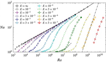
Figure 1 shows
 $Nu$
as a function of
 $Ra$
for both rotating and non-rotating cases. In rotating convection, the onset is delayed and the critical Rayleigh number
 $Ra_{c}$
increases with decreasing Ekman number. Close to critical,
 $Nu$
initially increases slowly and roughly linearly with
 $Ra$
(dashed line). Beyond this weakly nonlinear regime of rotating convection, i.e. when
 $Nu\gtrsim 2$
, the heat transport increases more rapidly with
 $Ra$
than in the non-rotating RBC (dotted-dashed line). This behaviour is reminiscent to that observed in plane layer studies (e.g. Rossby Reference Rossby1969; King et al.
Reference King, Stellmach, Noir, Hansen and Aurnou2009; Schmitz & Tilgner Reference Schmitz and Tilgner2009; Cheng et al.
Reference Cheng, Stellmach, Ribeiro, Grannan, King and Aurnou2015). Above a transitional Rayleigh number that will be determined below, the heat transfer data for each Ekman number then tend towards the non-rotating behaviour. As shown in our previous study (Gastine et al.
Reference Gastine, Wicht and Aurnou2015), the non-rotating data (
 $E=\infty$
) can be accurately described by a dissipation analysis that follows the Grossmann & Lohse (Reference Grossmann and Lohse2000) theory (black circles and solid black line). The non-rotating RBC thus defines an effective upper limit for the heat transport in rotating convection in spherical shells at large
 $Ra$
. In contrast to plane layer calculations, the spherical shell data do not exhibit any overshoot of rotating heat transfer beyond the non-rotating RBC scalings (Liu & Ecke Reference Liu and Ecke1997; Zhong et al.
Reference Zhong, Stevens, Clercx, Verzicco, Lohse and Ahlers2009).
Nusselt number as a function of the Rayleigh number with Ekman numbers denoted by symbol shape (and colour online). The dashed black line corresponds to the weakly nonlinear onset scaling
 $Nu-1=0.08\,(Ra/Ra_{c}-1)$
(3.2) discussed in § 3.1. The dot-dashed black line corresponds to the asymptotic scaling
 $Nu=0.15\,Ra^{3/2}E^{2}$
(3.10) in the rotation-dominated regime discussed in § 3.2. The solid black line corresponds to heat transfer scaling for non-rotating convection derived in Gastine et al. (Reference Gastine, Wicht and Aurnou2015). The four filled-in symbols correspond to the four cases highlighted in figure 2. The error bars correspond to one standard deviation from the time-averaged Nusselt number (i.e.
 $Nu\pm \unicode[STIX]{x1D70E}$
). For most of the numerical models, these error bars are smaller than the size of the symbols.

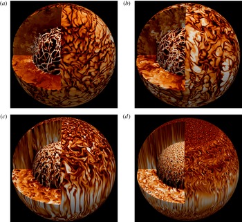
Meridional sections, equatorial cut and radial surfaces of the temperature fluctuations
 $\tilde{T}^{\prime }=\tilde{T}-\unicode[STIX]{x1D717}$
. The inner (outer) surface corresponds to the location of the inner (outer) thermal boundary layer
 $r=r_{i}+\unicode[STIX]{x1D706}_{T}^{i}$
(
 $r=r_{o}-\unicode[STIX]{x1D706}_{T}^{o}$
). Colour levels range from
 $-0.15$
(black) to
 $0.15$
(white). (a) corresponds to a non-rotating model with
 $Ra=10^{8}$
(Gastine et al.
Reference Gastine, Wicht and Aurnou2015). (b) corresponds to a numerical model with
 $E=10^{-4}$
and
 $Ro_{c}=1$
(case 146 in table 2). (c) corresponds to a numerical model with
 $E=10^{-5}$
and
 $Ro_{c}=0.17$
(case 191 in table 2). (d) corresponds to a numerical model with
 $E=10^{-6}$
and
 $Ro_{c}=0.05$
(case 219 in table 2).

To illustrate the diversity of the dynamical regimes in rotating spherical shell RBC, figure 2 shows equatorial, meridional and radial cuts of the dimensionless temperature fluctuations
 $\tilde{T}^{\prime }=\tilde{T}-\unicode[STIX]{x1D717}$
for four selected cases. The filled-in symbols in figure 1 indicate their positions in the
 $Nu-Ra$
parameter space. The image in figure 2(a) corresponds to a non-rotating model with
 $Ra=10^{8}$
. Due to an efficient turbulent mixing, the fluid bulk is nearly isothermalised and most of the temperature fluctuations take the form of thermal plumes that depart from the thin boundary layers. As visible on both spherical surfaces, the plume network is organised in long and thin sheet-like structures. Figure 2(b) corresponds to a numerical simulation with
 $E=10^{-4}$
and
 $Ra=10^{8}$
, i.e.
 $Ro_{c}=1$
. The turbulent flow remains essentially anisotropic and three-dimensional with a typical length scale comparable to that in the non-rotating model. At the connection points of the convective lanes network, we nevertheless observe the formation of vortical structures, which indicates the influence of the Coriolis force on the largest scale. Figure 2(c) shows a numerical model with
 $E=10^{-5}$
and
 $Ra=3\times 10^{8}$
. In the equatorial region, columnar structures aligned with the rotation axis are observed. At high latitudes, the integrity of the convective features is disrupted. This gradual loss of geostrophy is expected when the buoyancy forcing increases in strength with respect to the rotational constraint (here
 $Ro_{c}=0.17$
). The image in figure 2(d) corresponds to a numerical model with
 $E=10^{-6}$
and
 $Ro_{c}=0.05$
. As compared to the previous model, the stronger rotational influence on the flow results in a more pronounced alignment of the convective features with the rotation axis. Decreasing the Ekman number from
 $10^{-5}$
(figure 2
c) to
 $10^{-6}$
(figure 2
d) is accompanied by an obvious decrease of the typical convective flow length scale. In the rapidly rotating regime when
 $Ro_{c}\ll 1$
, Coriolis forces inhibit the turbulent mixing and the fluid bulk therefore departs from an isothermal state.
3.1 Weakly nonlinear regime of rotating convection
In rotating spherical shells, the convective flow at onset takes the form of prograde drifting thermal Rossby waves that first develop in the vicinity of the tangent cylinder (e.g. Busse Reference Busse1970; Dormy et al.
Reference Dormy, Soward, Jones, Jault and Cardin2004). The critical Rayleigh number
 $Ra_{c}$
and azimuthal wavenumber
 $m_{c}$
follow
 $$\begin{eqnarray}\quad Ra_{c}\sim E^{-4/3},\quad m_{c}\sim E^{-1/3}.\end{eqnarray}$$
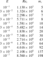
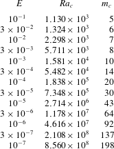
The exact values of
 $Ra_{c}$
and
 $m_{c}$
for the different Ekman numbers considered in this study are given in table 3. For marginally supercritical Rayleigh numbers, the weakly nonlinear perturbation analyses carried out by Busse & Or (Reference Busse and Or1986) and Gillet & Jones (Reference Gillet and Jones2006) predicted that the heat transport increases linearly with the supercriticality, i.e.:
 $$\begin{eqnarray}Nu-1\sim {\displaystyle \frac{Ra}{Ra_{c}}}-1.\end{eqnarray}$$
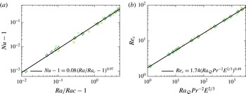
Figure 3(a) shows
 $Nu-1$
as a function of
 $Ra/Ra_{c}-1$
for the numerical simulations with
 $E\leqslant 3\times 10^{-5}$
and
 $Ra\leqslant 6\,Ra_{c}$
. The best fit to the data yields
 $Nu-1=0.076(\pm 0.003)(Ra/Ra_{c}-1)^{0.973(\pm 0.019)}$
. In spite of a remaining weak dependence on the Ekman number, the scaling (3.2) holds reasonably well for the numerical models with
 $Ra\leqslant 6\,Ra_{c}$
.
(a) Nusselt number
 $Nu-1$
as a function of
 $Ra/Ra_{c}-1$
. (b) Reynolds number
 $Re_{c}$
as a function of
 $Ra_{{\mathcal{Q}}}Pr^{-2}E^{2/3}$
. Only the cases with
 $E\leqslant 3\times 10^{-5}$
and
 $Ra\leqslant 6\,Ra_{c}$
are displayed in this figure. In both panels, the solid black lines correspond to the least-square fits to the data. The symbols have the same meaning as in figure 1.

A useful tool for establishing a scaling for the typical convective flow speed (
 $Re_{c}$
) is the linear relation between the viscous dissipation rate
 $\tilde{\unicode[STIX]{x1D716}}_{U}$
and the flux-based Rayleigh number
 $Ra_{{\mathcal{Q}}}$
given in (2.15). For a laminar flow close to the onset of convection,
 $\unicode[STIX]{x1D716}_{U}$
can be approximated by
 $$\begin{eqnarray}\unicode[STIX]{x1D716}_{U}\sim \unicode[STIX]{x1D708}\frac{U_{c}^{2}}{\ell _{\bot }^{2}},\end{eqnarray}$$
where
 $\ell _{\bot }$
is the typical flow length scale and
 $U_{c}$
the typical velocity. Close to the onset of convection,
 $\ell _{\bot }$
remains close to the critical azimuthal wavenumber, such that
 $$\begin{eqnarray}\ell _{\bot }/L\sim 1/m_{c}\sim E^{1/3}.\end{eqnarray}$$
Combining (2.15), (3.3) and (3.4) yields a scaling law for the convective flow speed
 $Re_{c}\sim U_{c}L/\unicode[STIX]{x1D708}$
 $$\begin{eqnarray}Re_{c}\sim Ra_{{\mathcal{Q}}}^{1/2}Pr^{-1}E^{1/3}.\end{eqnarray}$$
This scaling relation is sometimes called the Visco–Archimedean–Coriolis (hereafter VAC) scaling and can also be directly derived from the balance between these three forces (Aubert et al.
Reference Aubert, Brito, Nataf, Cardin and Masson2001; King & Buffett Reference King and Buffett2013; King et al.
Reference King, Stellmach and Buffett2013). Figure 3(b) shows
 $Re_{c}$
versus
 $Ra_{{\mathcal{Q}}}Pr^{-2}E^{2/3}$
for the numerical simulations with
 $E\leqslant 3\times 10^{-5}$
and
 $Ra\leqslant 6\,Ra_{c}$
. The least-square fit to the data yields
 $Re_{c}=1.744(\pm 0.041)(Ra_{{\mathcal{Q}}}\,E^{2/3})^{0.487(\pm 0.004)}$
, in excellent agreement with the theoretical scaling.
(a) Average flow length scale
 $\ell /L$
calculated using (2.14) as a function of the Ekman number for the numerical models close to the onset of convection with
 $Nu\leqslant 2$
and
 $E\leqslant 10^{-3}$
. (b) Corresponding compensated
 $\ell /L$
scaling. In both panels, the solid black lines correspond to
 $\ell /L=3\,E^{1/3}$
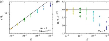
(3.4). The error bars illustrate the r.m.s. fluctuations and correspond to one standard deviation from the time averages. The symbols have the same meaning as in figure 1.

Figure 4(a) shows the average flow length scale
 $\ell /L$
plotted as a function of
 $E$
for the numerical models close to the onset of convection. The typical scale of convection gradually approaches the theoretical scaling
 $\ell /L\sim E^{1/3}$
when
 $E\leqslant 10^{-5}$
and the additional
 $Ra$
dependence vanishes. The compensated scaling displayed in figure 4(b) suggests the asymptotic scaling
 $\ell \simeq 3\,E^{1/3}\,L$
. The cases with the largest Ekman number (i.e.
 $E\geqslant 10^{-4}$
) significantly depart from this asymptotic law. This is not surprising since the scaling
 $m_{c}\sim E^{-1/3}$
is expected to hold for asymptotically small Ekman numbers (see table 3).
3.2 Nonlinear regime of rotating convection
3.2.1 Nusselt number scaling
As can be seen on figure 1, the weakly nonlinear scaling (3.2) provides an accurate description of the heat transport behaviour up to
 $Nu\simeq 1.5$
, which approximately corresponds to
 $Ra\simeq 6\,Ra_{c}$
. When
 $Nu>2$
, the heat transport increases much more rapidly and enters the nonlinear regime of rotating convection.
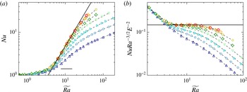
(a) Nusselt number as a function of
 $\widetilde{Ra}=RaE^{4/3}$
. (b) Corresponding compensated
 $Nu$
scaling. In both panels, the solid black line corresponds to the scaling
 $Nu=0.15\,Ra^{3/2}E^{2}$
(3.10). For clarity, only the cases with
 $E\leqslant 10^{-3}$
and
 $\widetilde{Ra}<200$
are displayed in this figure. The symbols have the same meaning as in figure 1.

The plane layer numerical simulations of rotating convection by King et al. (Reference King, Stellmach and Aurnou2012) and Stellmach et al. (Reference Stellmach, Lischper, Julien, Vasil, Cheng, Ribeiro, King and Aurnou2014) as well as the asymptotically reduced theoretical models by Julien et al. (Reference Julien, Knobloch, Rubio and Vasil2012a
) indicate that the convective heat flux only depends on the supercriticality
 $Ra/Ra_{c}$
when
 $Ro_{c}\ll 1$
. To check whether our numerical calculations actually support such a behaviour at low Ekman numbers, figure 5(a) shows
 $Nu$
as a function of
 $\widetilde{Ra}=RaE^{4/3}$
, since
 $Ra_{c}\sim E^{-4/3}$
. For
 $\widetilde{Ra}<6$
,
 $Nu$
slowly increases with the Rayleigh number and follows the previously described weakly nonlinear regime. Beyond this point, a fast steepening of the slope is observed and the function
 $Nu=f(\widetilde{Ra})$
starts to show an additional dependence on
 $E$
: while the large Ekman number cases quickly depart from a pure function of
 $\widetilde{Ra}$
, the low Ekman number simulations continue to follow a law of the form
 $Nu=f(\widetilde{Ra})$
up to higher
 $\widetilde{Ra}$
values. The exact location of this departure point gradually shifts to increasing
 $\widetilde{Ra}$
with decreasing
 $E$
. Figure 5(b) shows the compensated scalings of
 $Nu$
and reveals that the steepest part of the heat transfer law approaches the diffusivity-free scaling
 $Nu=0.15\widetilde{Ra}^{3/2}$
, at least in the range
 $6\leqslant \widetilde{Ra}\leqslant 20$
. To further assess the validity domain of the diffusivity-free scaling (1.3) in our numerical dataset, we introduce the local effective exponents
 $\unicode[STIX]{x1D6FC}_{eff}$
and
 $\unicode[STIX]{x1D6FD}_{eff}$
of the
 $Nu(Ra,E)$
law:
 $$\begin{eqnarray}\unicode[STIX]{x1D6FC}_{eff}=\left(\frac{\unicode[STIX]{x2202}\ln Nu}{\unicode[STIX]{x2202}\ln Ra}\right)_{E};\quad \unicode[STIX]{x1D6FD}_{eff}=\left(\frac{\unicode[STIX]{x2202}\ln Nu}{\unicode[STIX]{x2202}\ln E}\right)_{Ra}.\end{eqnarray}$$
The local exponent
 $\unicode[STIX]{x1D6FD}_{eff}$
is unfortunately difficult to constrain since our dataset only samples sparse variations of the Ekman number (half-decade sampling). However, the dense coverage in
 $Ra$
for each Ekman number subset allows to estimate the variations of
 $\unicode[STIX]{x1D6FC}_{eff}$
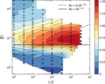
. Figure 6 shows isocontours of
 $\unicode[STIX]{x1D6FC}_{eff}$
in a
 $(1/E,\widetilde{Ra})$
-plane. Beyond the weakly nonlinear regime delimited by the horizontal solid black line, the effective slope gradually increases with decreasing
 $E$
. It reaches a maximum value
 $\unicode[STIX]{x1D6FC}_{eff}\simeq 3/2$
for a small region around
 $E\lesssim 10^{-6}$
and
 $\widetilde{Ra}\simeq 10$
.
Isocontours of the local effective exponent
 $\unicode[STIX]{x1D6FC}_{eff}$
of the
 $Nu=Ra^{\unicode[STIX]{x1D6FC}_{eff}}E^{\unicode[STIX]{x1D6FD}_{eff}}$
scaling in the
 $(1/E,\widetilde{Ra})$
-plane. The symbol shape corresponds to the Ekman number as in the previous figures, while the symbol colour scales here with the value of local slope
 $\unicode[STIX]{x1D6FC}_{eff}$
. The solid black line corresponds to the upper limit of the weakly nonlinear regime
 $Ra=6\,Ra^{4/3}$
, while the dashed black line corresponds to the dynamical boundary
 $Ra=0.4\,E^{-8/5}$
derived in figure 7.

The numerical simulations carried out by Cheng et al. (Reference Cheng, Stellmach, Ribeiro, Grannan, King and Aurnou2015) in Cartesian coordinates revealed a continuous increase of the local exponent
 $\unicode[STIX]{x1D6FC}_{eff}$
with decreasing
 $E$
and exhibit much steeper scaling beyond
 $\unicode[STIX]{x1D6FC}_{eff}\simeq 3$
(see also Stellmach et al.
Reference Stellmach, Lischper, Julien, Vasil, Cheng, Ribeiro, King and Aurnou2014; Kunnen et al.
Reference Kunnen, Ostilla-Mónico, van der Poel, Verzicco and Lohse2016). This phenomenon has been attributed to the sizeable role of Ekman pumping that enhances the heat transfer even in the low Ekman number regime (Julien et al.
Reference Julien, Aurnou, Calkins, Knobloch, Marti, Stellmach and Vasil2016). This steep scaling is not observed in absence of Ekman boundary layers, for instance when stress-free mechanical boundary conditions are adopted (Barker et al.
Reference Barker, Dempsey and Lithwick2014; Stellmach et al.
Reference Stellmach, Lischper, Julien, Vasil, Cheng, Ribeiro, King and Aurnou2014; Kunnen et al.
Reference Kunnen, Ostilla-Mónico, van der Poel, Verzicco and Lohse2016; Plumley et al.
Reference Plumley, Julien, Marti and Stellmach2016). In that case, local exponents close to
 $\unicode[STIX]{x1D6FC}_{eff}\simeq 3/2$
are recovered at low Ekman numbers.
The scaling exponents obtained in our simulations in spherical geometry for comparable Ekman numbers
 $E=O(10^{-7})$
remain bounded by the diffusivity-free scaling
 $\unicode[STIX]{x1D6FC}_{eff}=3/2$
(see also King et al.
Reference King, Soderlund, Christensen, Wicht and Aurnou2010). Although a further increase of
 $\unicode[STIX]{x1D6FC}_{eff}$
for
 $E<3\times 10^{-7}$
cannot be a priori ruled out, the compensated scaling shown in figure 5(b) suggests a gradual approach to
 $\unicode[STIX]{x1D6FC}=3/2$
, which seems to leave little room for further increase. This suggests that our simulations approach the asymptotic diffusivity-free behaviour for the parameter range
 $E\leqslant 10^{-6}$
and
 $6\leqslant \widetilde{Ra}\leqslant 20$
.
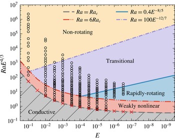
Clearly however, the validity domain of the diffusivity-free scaling (1.3) remains relatively narrow in our set of numerical models. Beyond the steep scaling with
 $\unicode[STIX]{x1D6FC}_{eff}\simeq 3/2$
, our numerical calculations show a transition to a shallower heat transfer scaling at larger supercriticality
 $\widetilde{Ra}$
. The characterisation of the upper bound of the rotation-dominated regime of rotating convection has been a long-standing question. The ratio of the global-scale Coriolis and buoyancy forces, approximated by the value of
 $Ro_{c}$
, has long been postulated to control the transition from rotation-dominated convection to non-rotating convection (e.g. Gilman Reference Gilman1977; Zhong & Ahlers Reference Zhong and Ahlers2010; Stevens, Clercx & Lohse Reference Stevens, Clercx and Lohse2013). Using a combination of laboratory experiments and local numerical simulations in Cartesian coordinates, King et al. (Reference King, Stellmach, Noir, Hansen and Aurnou2009) however demonstrated that a simple
 $Ro_{c}$
criterion does not correctly capture the regime transition, which happens while the bulk Rossby number is still much smaller than unity (see also Cheng et al.
Reference Cheng, Stellmach, Ribeiro, Grannan, King and Aurnou2015). They instead suggested that this transition is controlled by the competing thickness of the thermal and Ekman boundary layers. The resulting cross-over was found to follow
 $RaE^{3/2}\sim 1$
(King et al.
Reference King, Stellmach and Aurnou2012). However, numerical experiments that employed stress-free boundary conditions, in which viscous boundary layers are not present, yield a similar regime transition, which questions the role of the Ekman layer on the regime change (e.g. Schmitz & Tilgner Reference Schmitz and Tilgner2009).
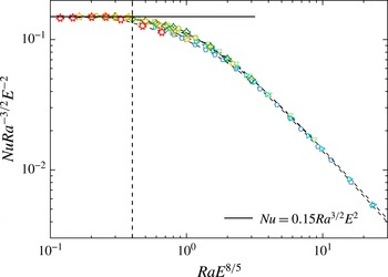
Nusselt number compensated by
 $Ra^{3/2}E^{2}$
as a function of
 $RaE^{8/5}$
. Only the cases with
 $E\leqslant 3\times 10^{-4}$
and
 $Nu\geqslant 2$
are displayed in this figure. The solid black line corresponds to the diffusivity-free scaling
 $Nu=0.15\,Ra^{3/2}E^{2}$
(3.10) already displayed in figure (5), while the vertical line corresponds to the dynamical boundary scaling
 $RaE^{8/5}=0.4$
. The symbols have the same meaning as in figure 1.

Julien et al. (Reference Julien, Rubio, Grooms and Knobloch2012b
) thus argued that the transition from rotationally constrained to what they call ‘rotationally influenced’ convection is rather controlled by the dynamics of the thermal boundary layers. In particular, they proposed that the diffusion-free scaling (1.3) breaks down when the thermal boundary layer is no longer in geostrophic balance. In other words,
 $Nu\sim \widetilde{Ra}^{3/2}$
would hold as long as the local convective Rossby number in the thermal boundary layer
 $Ro_{\unicode[STIX]{x1D706}}$
remains smaller than unity. The definition of
 $Ro_{\unicode[STIX]{x1D706}}$
leads to
 $$\begin{eqnarray}Ro_{\unicode[STIX]{x1D706}}=\frac{Ra_{\unicode[STIX]{x1D706}}^{1/2}\,E_{\unicode[STIX]{x1D706}}}{Pr^{1/2}}=\frac{(\unicode[STIX]{x1D6FC}_{T}g\unicode[STIX]{x0394}T_{\unicode[STIX]{x1D706}})^{1/2}}{\unicode[STIX]{x1D6FA}\unicode[STIX]{x1D706}^{1/2}},\end{eqnarray}$$
where
 $\unicode[STIX]{x1D706}$
is the thermal boundary layer thickness. Since
 $$\begin{eqnarray}Nu\sim \frac{\unicode[STIX]{x0394}T_{\unicode[STIX]{x1D706}}}{\unicode[STIX]{x1D706}}\frac{L}{\unicode[STIX]{x0394}T},\end{eqnarray}$$
using (1.3),
 $Ro_{\unicode[STIX]{x1D706}}\sim 1$
thus yields
 $$\begin{eqnarray}Ra\,E^{8/5}Pr^{-3/5}\sim 1.\end{eqnarray}$$
To test the applicability of this transition parameter, figure 7 shows the heat transfer data normalised by the diffusivity-free scaling (1.3),
 $NuRa^{-3/2}E^{-2}$
, versus
 $RaE^{8/5}$
for the numerical models with
 $E\leqslant 3\times 10^{-4}$
and
 $Nu\geqslant 2$
. The numerical simulations that fulfil
 $RaE^{8/5}<0.4$
lie very close to the geostrophic scaling (1.3). A best fit to the 16 cases that satisfy this criterion indeed yields
 $NuRa^{-3/2}E^{-2}=0.149(\pm 0.002)$
. The combination of the two criteria
 $RaE^{4/3}>6$
and
 $RaE^{8/5}<0.4$
defines a wedge in the parameter space highlighted by the two black lines visible in figure 6 where the scaling
 $$\begin{eqnarray}Nu=0.149(\pm 0.002)Ra^{3/2}E^{2}\end{eqnarray}$$
holds. The transition parameter (3.9) introduced by Julien et al. (Reference Julien, Rubio, Grooms and Knobloch2012b ) thus enables us to successfully demarcate the rotation-dominated regime and to efficiently collapse the heat transfer data across the regime transition.
3.2.2 Reynolds number scaling
To establish a scaling relation for the typical convective flow speed
 $Re_{c}$
, we examine first the variations of the viscous dissipation rate
 $\unicode[STIX]{x1D716}_{U}$
. In the limit of vanishing Ekman number, the viscous dissipation is expected to primarily occur in the bulk of the fluid (Busse Reference Busse1970). However, in the parameter range currently accessible to numerical models (i.e.
 $E\geqslant O(10^{-7})$
), dissipation by friction through the Ekman boundary layers might still contribute substantially to the total viscous dissipation rate (e.g. Aubert et al.
Reference Aubert, Brito, Nataf, Cardin and Masson2001). We thus follow the same strategy that has been fruitfully introduced by Grossmann & Lohse (Reference Grossmann and Lohse2000) for non-rotating RBC and decompose the viscous dissipation rate into a fluid bulk contribution
 $\unicode[STIX]{x1D716}_{U}^{bu}$
and a boundary layer contribution
 $\unicode[STIX]{x1D716}_{U}^{bl}$
:
 $$\begin{eqnarray}\unicode[STIX]{x1D716}_{U}=\unicode[STIX]{x1D716}_{U}^{bu}+\unicode[STIX]{x1D716}_{U}^{bl}=\frac{\unicode[STIX]{x1D708}}{V}\left(\int _{{\mathcal{T}}}(\unicode[STIX]{x1D735}\times \boldsymbol{u})^{2}\text{d}V+\int _{V\setminus {\mathcal{T}}}(\unicode[STIX]{x1D735}\times \boldsymbol{u})^{2}\text{d}V\right),\end{eqnarray}$$
where the integration domain is defined by
 ${\mathcal{T}}=\{r_{i}+\unicode[STIX]{x1D706}_{U}^{i}\leqslant r\leqslant r_{o}-\unicode[STIX]{x1D706}_{U}^{o};0\leqslant \unicode[STIX]{x1D703}\leqslant \unicode[STIX]{x03C0};0\leqslant \unicode[STIX]{x1D719}\leqslant 2\unicode[STIX]{x03C0}\}$
, where
 $\unicode[STIX]{x1D706}_{U}^{i}$
(
 $\unicode[STIX]{x1D706}_{U}^{o}$
) are the thicknesses of the inner (outer) viscous boundary layer. We then establish scaling relations for the two contributions
 $\unicode[STIX]{x1D716}_{U}^{bu}$
and
 $\unicode[STIX]{x1D716}_{U}^{bl}$
as functions of
 $Re_{c}$
and
 $E$
, starting with the kinetic dissipation rate in the bulk of the fluid which can be estimated by
 $$\begin{eqnarray}\unicode[STIX]{x1D716}_{U}^{bu}\sim \unicode[STIX]{x1D708}\frac{U_{c}^{2}}{\ell _{diss}^{2}},\end{eqnarray}$$
where
 $\ell _{diss}$
is the viscous dissipation length scale defined such that the local Reynolds number associated with this length scale is unity, i.e.
 $u_{diss}\,\ell _{diss}/\unicode[STIX]{x1D708}\sim 1$
. Following Davidson (Reference Davidson2013), we also introduce a small-scale vorticity
 $\unicode[STIX]{x1D714}_{diss}$
defined by
 $\unicode[STIX]{x1D714}_{diss}\sim u_{diss}/\ell _{diss}$
, which yields
 $$\begin{eqnarray}\unicode[STIX]{x1D716}_{U}^{bu}\sim U_{c}^{2}\,\unicode[STIX]{x1D714}_{diss}.\end{eqnarray}$$
At this stage, the study of the viscous dissipation rate needs to be complemented by a force balance analysis in order to estimate the scaling of
 $\unicode[STIX]{x1D714}_{diss}$
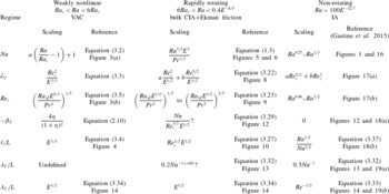
. A viscosity-free scaling of rotating convection was first proposed by Stevenson (Reference Stevenson1979) and Ingersoll & Pollard (Reference Ingersoll and Pollard1982) and later further developed by Aubert et al. (Reference Aubert, Brito, Nataf, Cardin and Masson2001). This scaling, known as the inertial scaling of rapidly rotating convection, hypothesises a triple force balance between Coriolis, inertia and Archimedean force (hereafter CIA). Taking the curl of the Navier–Stokes equation (2.2) in its dimensional form, the CIA triple balance yields
 $$\begin{eqnarray}\unicode[STIX]{x1D6FA}\frac{\unicode[STIX]{x2202}\boldsymbol{u}}{\unicode[STIX]{x2202}z}\sim \boldsymbol{u}\boldsymbol{\cdot }\unicode[STIX]{x1D735}\unicode[STIX]{x1D74E}\sim \unicode[STIX]{x1D735}\times (\unicode[STIX]{x1D6FC}_{T}Tg\,\boldsymbol{e}_{r}),\end{eqnarray}$$
where the factor two in the vortex stretching term has been omitted. We now introduce the two integral length scales
 $\ell _{\bot }$
and
 $\ell _{/\!/}$
, respectively perpendicular and parallel to the rotation axis. Since rapidly rotating convective patterns take the form of columnar structures aligned with the rotation axis,
 $\ell _{\bot }\ll \ell _{/\!/}$
. Denoting
 $U_{c}$
the typical velocity,
 $\unicode[STIX]{x1D6E9}$
the typical thermal perturbation and
 $\unicode[STIX]{x1D714}_{c}$
the typical vorticity, one gets
 $$\begin{eqnarray}\unicode[STIX]{x1D6FA}\,\frac{U_{c}}{\ell _{/\!/}}\sim U_{c}\,\frac{\unicode[STIX]{x1D714}_{c}}{\ell _{\bot }}\sim \unicode[STIX]{x1D6FC}_{T}g\,\frac{\unicode[STIX]{x1D6E9}}{\ell _{\bot }}.\end{eqnarray}$$
We now assume that the axial dimension of the convection rolls
 $\ell _{/\!/}$
can be approximated by the container length scale
 $L$
. This assumption, combined with the balance between Coriolis force and inertia in (3.15), yields
 $$\begin{eqnarray}\ell _{\bot }/L\sim \unicode[STIX]{x1D714}_{c}/\unicode[STIX]{x1D6FA}.\end{eqnarray}$$
We further assume that the convective heat flux per unit area
 ${\mathcal{Q}}$
scales as
 $$\begin{eqnarray}{\mathcal{Q}}\sim \unicode[STIX]{x1D70C}c_{p}U_{c}\unicode[STIX]{x1D6E9}\sim (Nu-1)\unicode[STIX]{x1D705}\unicode[STIX]{x1D70C}c_{p}\unicode[STIX]{x0394}T/L,\end{eqnarray}$$
which implies that the correlation between thermal perturbation and velocity are independent of
 $E$
,
 $Pr$
and
 $Ra$
(Gillet & Jones Reference Gillet and Jones2006). The balance between inertia and buoyancy in (3.15) then leads to
 $$\begin{eqnarray}Ra_{{\mathcal{Q}}}Pr^{-2}\sim (L^{4}/\unicode[STIX]{x1D708}^{3})\,U_{c}^{2}\,\unicode[STIX]{x1D714}_{c}.\end{eqnarray}$$
Since on time average
 $(\unicode[STIX]{x1D708}^{3}/L^{4})\,\unicode[STIX]{x1D716}_{U}\sim Ra_{{\mathcal{Q}}}Pr^{-2}$
, it follows from (3.13)
 $\unicode[STIX]{x1D714}_{diss}\sim \unicode[STIX]{x1D714}_{c}$
. The proportionality relation between the typical time scale at the integral length
 $\ell _{\bot }$
and at the dissipation scale
 $\ell _{diss}$
is a distinctive feature of two-dimensional turbulence (e.g. Davidson Reference Davidson2015). Finally assuming that
 $\unicode[STIX]{x1D714}_{c}\sim U_{c}/\ell _{\bot }$
, one can derive the following expression for the viscous dissipation rate in the fluid bulk
 $$\begin{eqnarray}\unicode[STIX]{x1D716}_{U}^{bu}=\frac{U_{c}^{3}}{\ell _{\bot }}=\frac{\unicode[STIX]{x1D708}^{3}}{L^{4}}\,\frac{Re_{c}^{5/2}}{E^{1/2}}.\end{eqnarray}$$
(a) Dimensionless viscous dissipation rate
 $\tilde{\unicode[STIX]{x1D716}}_{U}$
as a function of the Reynolds number
 $Re_{c}$
. (b) Corresponding compensated
 $\tilde{\unicode[STIX]{x1D716}}_{U}$
scaling. The solid black lines correspond to the theoretical scaling derived in (3.22) with
 $a=0.066$
and
 $b=4.843$
. Only the cases that fulfil the conditions
 $Nu>2$
and
 $RaE^{8/5}<1$
have been selected on this figure. The error bars illustrate the r.m.s. fluctuations and correspond to one standard deviation from the time averages. The symbols have the same meaning as in figure 1.

The same procedure can be applied to the viscous dissipation in the Ekman boundary layers with the difference that the typical length scale is now the boundary layer thickness
 $\unicode[STIX]{x1D706}_{U}$
. Furthermore, the dissipation occurs only in the fraction of the fluid volume occupied by the viscous boundary layers. In the limit of
 $\unicode[STIX]{x1D706}_{U}\ll L$
, this volume fraction can be approximated by the ratio
 $\unicode[STIX]{x1D706}_{U}/L$
, thus neglecting any curvature effect. This yields
 $$\begin{eqnarray}\unicode[STIX]{x1D716}_{U}^{bl}\sim \unicode[STIX]{x1D708}\frac{U_{c}^{2}}{\unicode[STIX]{x1D706}_{U}^{2}}\,\frac{\unicode[STIX]{x1D706}_{U}}{L}.\end{eqnarray}$$
Since
 $\unicode[STIX]{x1D706}_{U}/L\sim E^{1/2}$
(see below in § 3.2.5), the viscous dissipation by friction through the boundary layers can be expressed by
 $$\begin{eqnarray}\unicode[STIX]{x1D716}_{U}^{bl}\sim \frac{\unicode[STIX]{x1D708}^{3}}{L^{4}}\,\frac{Re_{c}^{2}}{E^{1/2}}.\end{eqnarray}$$
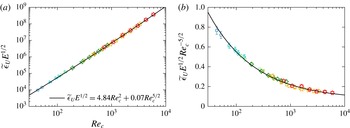
Combining (3.19) and (3.21) allows us to derive the following scaling behaviour for the dimensionless viscous dissipation rate
 $$\begin{eqnarray}\tilde{\unicode[STIX]{x1D716}}_{U}=a\,\frac{Re_{c}^{5/2}}{E^{1/2}}+b\,\frac{Re_{c}^{2}}{E^{1/2}}.\end{eqnarray}$$
To test the validity of this scaling, we calculate
 $\tilde{\unicode[STIX]{x1D716}}_{U}$
and
 $Re_{c}$
in our numerical simulations and directly fit the expression (3.22). This leaves only the two prefactors
 $a$
and
 $b$
as free fitting parameters. Figure 8(a) shows
 $\tilde{\unicode[STIX]{x1D716}}_{U}E^{1/2}$
as a function of
 $Re_{c}$
for the 41 cases that fulfil
 $Nu>2$
and
 $RaE^{8/5}<1$
. The best fit to the numerical data yields
 $a=0.066(\pm 0.003)$
and
 $b=4.843(\pm 0.096)$
. The expression (3.22) provides an excellent agreement with the data, further confirmed by the bulk compensated scaling
 $\tilde{\unicode[STIX]{x1D716}}_{U}E^{1/2}Re_{c}^{-5/2}$
shown in figure 8(b). Explicitly including the viscous friction that occurs in the Ekman boundary layers thus allows to very accurately describe the numerical data over a broad range of parameter
 $3\times 10^{-4}\leqslant E\leqslant 3\times 10^{-7}$
,
 $10^{2}\leqslant Re_{c}\leqslant 10^{4}$
. We also note that a stricter restriction to the 16 turbulent cases that satisfy the criterion
 $RaE^{8/5}<0.4$
and thus lie within the wedge displayed in figure (6) yields very similar values for
 $a$
and
 $b$
. The expression (3.22) also allows to estimate the transition value of
 $Re_{c}$
beyond which the viscous dissipation that occurs in the interior of the fluid will dominate the dissipation in boundary layers. Figure 8(b) demonstrates that our dataset nearly reaches this point where the bulk scaling alone provides a good description. Using the best fitting parameters
 $a$
and
 $b$
yields
 $Re_{c}=(b/a)^{2}\simeq 5500$
. Beyond this value, the viscous dissipation in the Ekman layers becomes secondary and the dynamical behaviour will then gradually tend towards the inertial scaling of rotating convection.
(a) Reynolds number
 $Re_{c}$
as a function of
 $Ra_{{\mathcal{Q}}}Pr^{-2}E^{1/2}$
. (b) Corresponding compensated
 $Re_{c}$
scaling. The solid black lines correspond to the theoretical scaling derived in (3.26), while the dashed black lines correspond to the least-square fit to the data. Only the cases that fulfil the conditions
 $Nu>2$
and
 $RaE^{8/5}<1$
have been selected on this figure. The error bars illustrate the r.m.s. fluctuations and correspond to one standard deviation from the time averages. The symbols have the same meaning as in figure 1.

Assuming that the viscous dissipation either entirely occurs in the fluid bulk (i.e.
 $\unicode[STIX]{x1D716}_{U}\simeq \unicode[STIX]{x1D716}_{U}^{bu}$
) or in the Ekman layers (i.e.
 $\unicode[STIX]{x1D716}_{U}\simeq \unicode[STIX]{x1D716}_{U}^{bl}$
) allows one to define the two end-member scaling relations:
 $$\begin{eqnarray}Re_{c}^{bu}\leqslant Re_{c}\leqslant Re_{c}^{bl},\end{eqnarray}$$
where
 $$\begin{eqnarray}Re_{c}^{bl}\sim Ra_{{\mathcal{Q}}}^{1/2}Pr^{-1}E^{1/4}\end{eqnarray}$$
and
 $$\begin{eqnarray}Re_{c}^{bu}\sim Ra_{{\mathcal{Q}}}^{2/5}Pr^{-4/5}E^{1/5}.\end{eqnarray}$$
We note that (3.25) corresponds to the convective velocity scaling classically obtained in the CIA triple balance (e.g. Aubert et al.
Reference Aubert, Brito, Nataf, Cardin and Masson2001; Gillet & Jones Reference Gillet and Jones2006; Barker et al.
Reference Barker, Dempsey and Lithwick2014), while the scaling (3.24) has the same dependence on
 $Ra_{{\mathcal{Q}}}$
as the VAC triple balance (3.5) but carries a different
 $E$
-scaling exponent. Once
 $a$
and
 $b$
have been determined, the equation (3.22) can be numerically solved to derive the combined scaling law for
 $Re_{c}$
:
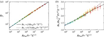
 $$\begin{eqnarray}Re_{c}=f(Ra_{{\mathcal{Q}}}Pr^{-2}E^{1/2}).\end{eqnarray}$$
For comparison purposes, we also compute a simple best fit to the data which yields
 $Re_{c}=0.708(\pm 0.017)(Ra_{{\mathcal{Q}}}Pr^{-2}E^{1/2})^{0.473\pm 0.002}$
. Figure 9(a) shows
 $Re_{c}$
versus
 $Ra_{{\mathcal{Q}}}Pr^{-2}E^{1/2}$
for the 41 cases already shown in figure 8, while figure 9(b) shows the corresponding bulk compensated scaling.
Previous parameter studies of rotating convection in spherical shells either carried out under the quasi-geostrophic assumption (Gillet & Jones Reference Gillet and Jones2006; Guervilly Reference Guervilly2010) or in fully three-dimensional models (Christensen Reference Christensen2002; King & Buffett Reference King and Buffett2013) obtained steeper exponents than the
 $2/5$
scaling expected in the classical CIA balance (3.25). This discrepancy has usually been attributed to the significant role played by viscosity in numerical models and thus prompted several authors to rather describe their dataset using the VAC scaling hypothesis (3.5). Since the scaling exponents are relatively close to each other,
 $2/5$
versus
 $1/2$
regarding the dependence on
 $Ra_{{\mathcal{Q}}}$
, discriminating one scaling from another remains however a difficult task (King & Buffett Reference King and Buffett2013). (Note however that the Ekman number dependence is not the same for these two scalings.) Here we show that the separation of
 $\unicode[STIX]{x1D716}_{U}$
into boundary layers and bulk contributions allows us to very accurately describe the numerical data. Moreover, in the range of
 $Re_{c}$
covered by our numerical dataset (i.e.
 $10^{2}\leqslant Re_{c}<10^{4}$
), the simple power law
 $Re_{c}=0.708(\pm 0.017)(Ra_{{\mathcal{Q}}}Pr^{-2}E^{1/2})^{0.473\pm 0.002}$
provides a statistically nearly indiscernible fit quality from the scaling theory (3.26). Deviations only become more significant at the high end of the parameter range, where the power law fails to accurately capture the complex dependence of
 $Re_{c}$
upon
 $Ra_{{\mathcal{Q}}}Pr^{-2}E^{1/2}$
. This explains why previous analyses that reduced the scaling behaviours of
 $Re_{c}$
to such simple power laws obtained scaling exponents robustly larger than
 $2/5$
(e.g. Gillet & Jones Reference Gillet and Jones2006; King & Buffett Reference King and Buffett2013).
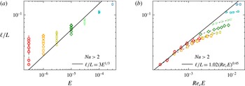
(a) Average flow length scale
 $\ell /L$
calculated using (2.14) as a function of the Ekman number for the numerical models with
 $E\leqslant 3\times 10^{-4}$
and
 $Nu>2$
. For comparison, the weakly nonlinear scaling obtained in figure 4 has been plotted as a solid black line. (b) Corresponding compensated
 $\ell /L$
scaling. Only the 41 cases that satisfy
 $Nu>2$
and
 $RaE^{8/5}<1$
have been selected on this figure. The solid black line corresponds to the best fit to the cases with
 $E=3\times 10^{-7}$
. The error bars illustrate the r.m.s. fluctuations and correspond to one standard deviation from the time averages. The symbols have the same meaning as in figure 1.

3.2.3 Flow length scales and interior temperature gradients
Using the equations (3.16) and (3.25), the inertial theory of rotating convection predicts the following scaling for the integral flow length scale
 $\ell _{\bot }$
 $$\begin{eqnarray}\ell _{\bot }/L\sim (U_{c}/\unicode[STIX]{x1D6FA}L)^{1/2}\sim (Re_{c}E)^{1/2},\end{eqnarray}$$
which is generally referred to as the Rhines scaling (Rhines Reference Rhines1975). Using the numerical models computed by Christensen & Aubert (Reference Christensen and Aubert2006), several analyses of the typical flow length scale suggest that the VAC scaling (3.4) might possibly hold beyond the weakly nonlinear regime of rotating convection (e.g. King & Buffett Reference King and Buffett2013; Oruba & Dormy Reference Oruba and Dormy2014). Figure 10(a) shows the calculations of the average flow length scale
 $\ell /L$
plotted as a function of
 $E$
for the numerical models with
 $E\leqslant 3\times 10^{-4}$
and
 $Nu>2$
. The
 $\ell \sim E^{1/3}\,L$
scaling that accurately describes the numerical data close to onset of convection (see figure 4) fails to properly capture the length scale variations in the nonlinear regime. Especially, at low Ekman numbers (
 $E\leqslant 3\times 10^{-6}$
),
 $\ell$
exhibits a strong additional dependence on the convective forcing and increases with the supercriticality (see table 2 for details). Figure 10(b) shows the calculations of
 $\ell$
versus
 $Re_{c}E$
for the 41 numerical models already shown in figures 8 and 9. A best fit to the cases with
 $E=3\times 10^{-7}$
that fulfil
 $RaE^{8/5}<0.4$
yields
 $\ell /L=1.016(\pm 0.212)(Re_{c}E)^{0.45(\pm 0.027)}$
, reasonably close to the theoretical scaling (3.27). Since the dissipation that occurs in the boundary layers still plays a substantial role in the velocity scaling (3.22), it is not surprising that (3.27) is only approached for the lowest Ekman number considered in this study.
(a) Radial profile of the time and horizontally averaged temperature
 $\unicode[STIX]{x1D717}(r)$
for different convective Rossby number
 $Ro_{c}$
with a fixed Ekman number of
 $E=10^{-4}$
. The dot-dashed black line corresponds to the conductive temperature profile solution of (2.10). (b) Radial profile of the time and horizontally averaged temperature
 $\unicode[STIX]{x1D717}(r)$
for different Ekman numbers with approximately the same Nusselt number
 $10.3<Nu<11$
.

While non-rotating convection undergoes an efficient turbulent mixing which results in an isothermal fluid interior (e.g. Verzicco & Camussi Reference Verzicco and Camussi1999), the prominent role played by the Coriolis force in rotating convection impedes the mixing. Both experiments (e.g. Boubnov & Golitsyn Reference Boubnov and Golitsyn1990; Kunnen et al.
Reference Kunnen, Geurts and Clercx2010) and direct numerical simulations (e.g. Julien et al.
Reference Julien, Legg, McWilliams and Werne1996; King et al.
Reference King, Stellmach and Aurnou2012; Stellmach et al.
Reference Stellmach, Lischper, Julien, Vasil, Cheng, Ribeiro, King and Aurnou2014) have indeed revealed that a large-scale interior temperature gradient can be maintained in the rapidly rotating regime (see also Gillet & Jones Reference Gillet and Jones2006; King et al.
Reference King, Soderlund, Christensen, Wicht and Aurnou2010). Figure 11 shows the time- and horizontally averaged temperature profile
 $\unicode[STIX]{x1D717}(r)$
for several rotating and non-rotating models. At a fixed Ekman number, an increase of the supercriticality (figure 11
a) changes the temperature distribution from a nearly conductive state (solid orange line) to a nearly isothermal fluid bulk (dot-dashed line). At larger
 $Ro_{c}$
(broken lines), the rotational constraint decreases and thin thermal boundary layers start to emerge and tend to accommodate an increasing fraction of the temperature drop. As visible in figure 11(b), the transition from rotating to non-rotating convection is thus associated with a gradual lowering of the average temperature gradient and a transition to a physical regime where boundary layers entirely control the heat transfer.
(a) Temperature gradient at mid-shell radius
 $\unicode[STIX]{x1D6FD}_{T}$
versus
 $\widetilde{Ra}$
for the numerical models with
 $Nu>2$
and
 $E\leqslant 10^{-3}$
. (b) Absolute temperature gradient at mid-shell renormalised by
 $E^{-1/2}$
versus
 $NuRe_{c}^{-3/2}$
for the numerical models with
 $RaE^{8/5}<1$
and
 $Nu>2$
. The solid black line corresponds to the best fit to the data. The symbols have the same meaning as in figure 1.

Measuring the interior temperature gradient
 $\unicode[STIX]{x1D6FD}_{T}$
(2.13a,b
) thus helps to characterise the heat transfer regime. Figure 12(a) shows
 $\unicode[STIX]{x1D6FD}_{T}$
versus
 $\widetilde{Ra}$
for the set of numerical simulations with
 $E\leqslant 10^{-3}$
. An increase of the supercriticality
 $\widetilde{Ra}$
leads to a gradual decrease of
 $|\unicode[STIX]{x1D6FD}_{T}|$
. The thermal profiles in the fluid bulk tend to a thermally well-mixed interior (i.e. vanishing
 $\unicode[STIX]{x1D6FD}_{T}$
) when the rotational influence on the flow decreases. In contrast to the asymptotic calculations by Julien et al. (Reference Julien, Rubio, Grooms and Knobloch2012b
), our dataset does not show any evidence for a direct scaling relation between
 $\unicode[STIX]{x1D6FD}_{T}$
and
 $\widetilde{Ra}$
. However, following Stevenson (Reference Stevenson1979) and Barker et al. (Reference Barker, Dempsey and Lithwick2014), the interior temperature gradient can be estimated by
 $$\begin{eqnarray}\unicode[STIX]{x1D6FD}_{T}\sim \frac{\unicode[STIX]{x1D6E9}}{\ell _{\bot }}\frac{L}{\unicode[STIX]{x0394}T},\end{eqnarray}$$
in the rapidly rotating limit. Using (3.27) for the length scale scaling and approximating
 $\unicode[STIX]{x1D6E9}/\unicode[STIX]{x0394}T$
by
 $Nu/Re_{c}$
then yields
 $$\begin{eqnarray}\unicode[STIX]{x1D6FD}_{T}\sim Nu\,Re_{c}^{-3/2}E^{-1/2}.\end{eqnarray}$$
Figure 12(b) shows that this scaling provides a reasonable description of the 41 numerical cases already discussed in figures 8 and 9. The best fit to the data however gives a shallower exponent than expected from theory:
 $\unicode[STIX]{x1D6FD}_{T}E^{1/2}=0.643(\pm 0.027)(NuRe_{c}^{-3/2})^{0.812(\pm 0.005)}$
. This discrepancy is not surprising since the underlying
 $\ell _{\bot }$
scaling that enters (3.29) is only partially realised in our set of simulations (see figure 10). Lowering the Ekman number further might help to ascertain this scaling. Indeed, the local numerical calculations carried out in Cartesian coordinates by Barker et al. (Reference Barker, Dempsey and Lithwick2014) demonstrate the validity of (3.29) once the influence of the viscous boundary layers has been minimised. Replacing the expected asymptotic scalings for
 $Nu$
(1.3) and
 $Re_{c}$
(3.25) in (3.29) yields
 $\unicode[STIX]{x1D6FD}_{T}\sim Pr$
. This implies that
 $\unicode[STIX]{x1D6FD}_{T}$
should saturate on a constant value in the turbulent quasi-geostrophic regime of rotating convection. Local numerical calculations carried out in Cartesian coordinates by Stellmach et al. (Reference Stellmach, Lischper, Julien, Vasil, Cheng, Ribeiro, King and Aurnou2014) indeed obtain a saturation of
 $\unicode[STIX]{x1D6FD}_{T}$
for
 $E=O(10^{-7})$
and
 $\widetilde{Ra}\sim 100$
.
(a,b) Thermal boundary layer thickness at the inner (outer) boundary
 $\unicode[STIX]{x1D706}_{T}^{i}$
(
 $\unicode[STIX]{x1D706}_{T}^{o}$
) as a function of the Nusselt number. The solid black lines correspond to the theoretical scalings for non-rotating convection derived in Gastine et al. (Reference Gastine, Wicht and Aurnou2015). (c,d) Compensated
 $\unicode[STIX]{x1D706}_{T}^{i}/L$
(
 $\unicode[STIX]{x1D706}_{T}^{o}/L$
) scaling. The symbols have the same meaning as in figure 1.

3.2.4 Thermal boundary layers
Since the heat transport in the thermal boundary layers is controlled by diffusion, the Nusselt number provides an estimate for the ratio between the thermal boundary layer thickness and the related temperature drop:
 $$\begin{eqnarray}Nu=\unicode[STIX]{x1D702}\frac{\unicode[STIX]{x0394}T_{i}}{\unicode[STIX]{x1D706}_{T}^{i}}\frac{L}{\unicode[STIX]{x0394}T}=\frac{1}{\unicode[STIX]{x1D702}}\frac{\unicode[STIX]{x0394}T_{o}}{\unicode[STIX]{x1D706}_{T}^{o}}\frac{L}{\unicode[STIX]{x0394}T},\end{eqnarray}$$
where
 $\unicode[STIX]{x1D706}_{T}^{i}$
(
 $\unicode[STIX]{x1D706}_{T}^{o}$
) is the thickness of the thermal boundary layer at the inner (outer) boundary and
 $\unicode[STIX]{x0394}T_{i}$
(
 $\unicode[STIX]{x0394}T_{o}$
) is the associated temperature contrast. This yields the following scalings for the thermal boundary layer thicknesses at both boundaries:
 $$\begin{eqnarray}\frac{\unicode[STIX]{x1D706}_{T}^{i}}{L}=\unicode[STIX]{x1D702}\frac{\unicode[STIX]{x0394}T_{i}}{\unicode[STIX]{x0394}T}\frac{1}{Nu};\quad \frac{\unicode[STIX]{x1D706}_{T}^{o}}{L}=\frac{1}{\unicode[STIX]{x1D702}}\frac{\unicode[STIX]{x0394}T_{o}}{\unicode[STIX]{x0394}T}\frac{1}{Nu}.\end{eqnarray}$$
In non-rotating convection in spherical geometry, the thermal boundary layers are asymmetric and thus
 $\unicode[STIX]{x0394}T^{i}/\unicode[STIX]{x0394}T^{o}\neq 1$
. In a previous study, we demonstrated that the ratio
 $\unicode[STIX]{x0394}T^{i}/\unicode[STIX]{x0394}T^{o}$
only depends on the radius ratio
 $\unicode[STIX]{x1D702}$
and on the gravity profile
 $\tilde{g}(r)$
(Gastine et al.
Reference Gastine, Wicht and Aurnou2015). Thus, the scaling for the boundary layer thickness in non-rotating RBC is
 $$\begin{eqnarray}\unicode[STIX]{x1D706}_{T}^{i}/L\sim \unicode[STIX]{x1D706}_{T}^{o}/L\sim Nu^{-1},\end{eqnarray}$$
where only the scaling prefactors depend on the geometry and on the gravity distribution of the spherical shell. In rotating convection however, the temperature drops at each thermal boundary layer are likely to also depend on
 $Ra$
and
 $E$
and hence a non-trivial additional dependence on
 $Nu$
might be expected (see figure 11). Figure 13 shows the calculations of
 $\unicode[STIX]{x1D706}_{T}^{i}$
and
 $\unicode[STIX]{x1D706}_{T}^{o}$
using the slope-intersection method described in § 2.3 versus
 $Nu$
for both rotating and non-rotating simulations. As pointed out by Julien et al. (Reference Julien, Rubio, Grooms and Knobloch2012b
), other methods to estimate the thermal boundary layers in rotating convection might yield different thicknesses. A comparison between the values obtained from the slope-intersection method with the location of the peaks of the r.m.s. of the temperature fluctuations for a few selected cases however yield similar boundary layer thicknesses (for a comparison, see Gastine et al.
Reference Gastine, Wicht and Aurnou2015). Large Ekman number models (
 $E\geqslant 10^{-2}$
) essentially behave similarly to the non-rotating cases. At the inner boundary of the spherical shell, the cases with intermediate Ekman numbers
 $3\times 10^{-5}\leqslant E\leqslant 3\times 10^{-3}$
exhibit a lower prefactor and a slightly shallower slope than
 $Nu^{-1}$
particularly visible in the compensated plot displayed in figure 13(c). The cases with
 $E\leqslant 3\times 10^{-6}$
, however seem to follow again a scaling
 $\unicode[STIX]{x1D706}_{T}^{i}/L\sim Nu^{-1}$
, though with a much smaller prefactor (
 $\simeq 0.17$
instead of
 $\simeq 0.4$
) than the non-rotating cases. The thermal boundary layer at the outer boundary behaves quite differently. On average,
 $\unicode[STIX]{x1D706}_{T}^{o}$
remains much closer to the values found in the non-rotating models and can thus be roughly approximated by
 $\unicode[STIX]{x1D706}_{T}^{o}/L\sim Nu^{-1}$
. However, a secondary, intricate dependence on the Ekman number remains, as visible on the compensated scaling of
 $\unicode[STIX]{x1D706}_{T}^{o}$
displayed in figure 13(d). For both boundary layers, the
 $Nu^{-1}$
scaling thus provides an acceptable first-order approximation of the thermal boundary layer thickness measured by the slope-intersection method, though subtle dependences on the Ekman number can impinge on both the prefactor and the scaling exponent.
3.2.5 Viscous boundary layers
In the range of Rayleigh numbers explored here (
 $10^{3}\leqslant Ra\leqslant 10^{11}$
), the viscous boundary layers in non-rotating convection are usually assumed to be laminar and follow the Prandtl–Blasius boundary layer theory (Prandtl Reference Prandtl1905; Blasius Reference Blasius1908). Balancing the inertia of the fluid bulk with the viscous forces in the boundary layers yields
 $$\begin{eqnarray}\unicode[STIX]{x1D706}_{U}/L\sim Re^{-1/2}.\end{eqnarray}$$
In contrast, owing to the primary role of Coriolis force, the viscous boundary layers in rotating convection, called the Ekman layers, differ greatly from non-rotating convection. A scaling relation for the Ekman layers can be derived by considering a force balance between Coriolis force and viscosity in the limit of
 $E\rightarrow 0$
(e.g. Greenspan Reference Greenspan1968):
 $$\begin{eqnarray}\unicode[STIX]{x1D734}\times \boldsymbol{u}\sim \unicode[STIX]{x1D708}\unicode[STIX]{x1D6AB}\boldsymbol{u}\rightarrow \unicode[STIX]{x1D706}_{U}/L\sim E^{1/2}.\end{eqnarray}$$
Figure 14 shows the calculations of the viscous boundary layer thicknesses for both the inner and the outer spherical shell boundaries as a function of
 $Re_{c}$
and
 $E$
. Here we only examine the mean viscous boundary layer, though in spherical geometry the Ekman layer thickness might also depend on the latitude (Greenspan Reference Greenspan1968). When the Ekman number is large (
 $E\geqslant 3\times 10^{-3}$
), the influence of rotation on the viscous boundary layer remains secondary.
 $\unicode[STIX]{x1D706}_{U}^{i}$
and
 $\unicode[STIX]{x1D706}_{U}^{o}$
are then essentially the same as the non-rotating cases (figure 14
a,b). As already shown in our previous study (Gastine et al.
Reference Gastine, Wicht and Aurnou2015), when
 $Re_{c}\geqslant 250$
, the scaling exponents are in close agreement with the Prandtl–Blasius scaling (3.33). At lower Ekman numbers (
 $E\leqslant 3\times 10^{-5}$
), the viscous boundary layer thicknesses become almost independent of
 $Re_{c}$
and approach the theoretical scaling for Ekman layers (figure 14
c,d). Indeed, the best fit to the numerical cases that fulfil
 $RaE^{8/5}<1$
and
 $Nu>2$
yields
 $\unicode[STIX]{x1D706}_{U}^{i}/L=0.875(\pm 0.084)\,E^{0.465(\pm 0.008)}$
and
 $\unicode[STIX]{x1D706}_{U}^{o}/L=1.109(\pm 0.042)\,E^{0.497(\pm 0.003)}$
, in good agreement with (3.34).
(a,b) Viscous boundary layer thickness at the inner (outer) boundary
 $\unicode[STIX]{x1D706}_{U}^{i}$
(
 $\unicode[STIX]{x1D706}_{U}^{o}$
) as a function of
 $Re_{c}$
. The solid lines correspond to the scalings obtained for non-rotating convection derived in Gastine et al. (Reference Gastine, Wicht and Aurnou2015). (c,d) Viscous boundary layer thickness at the inner (outer) boundary as a function of the Ekman number. The solid black lines correspond to the best fit to the 41 cases that fulfil
 $RaE^{8/5}<1$
and
 $Nu>2$
. The symbols have the same meaning as in figure 1.

3.3 Transitional regime: from rotating to non-rotating convection
In the previous sections, we mainly explored the range of parameters where the convective flow is strongly constrained by rotation. We showed that the criterion
 $RaE^{8/5}\leqslant O(1)$
posited by Julien et al. (Reference Julien, Knobloch, Rubio and Vasil2012a
) provides an effective way to characterise the upper bound of this physical regime. Beyond this point, i.e. when
 $Ra>E^{-8/5}$
, convection is still influenced by rotation but no longer operates in the turbulent quasi-geostrophic regime. This defines the lower bound of the transitional regime of rotating convection. To illustrate the continuous variations of the physical properties within this regime, figure 15 shows isocontours of the local slope
 $\unicode[STIX]{x1D6FC}_{eff}$
of the Nusselt scaling in a
 $(Ra,Nu)$
-plane. Beyond the rapidly rotating regime of convection in which
 $\unicode[STIX]{x1D6FC}_{eff}\simeq 3/2$
(dark red area), a rapid decrease of the local exponent is observed. The heat transport is not characterised by one single scaling exponent
 $\unicode[STIX]{x1D6FC}_{eff}$
but rather exhibits continuous changes, similarly to what is observed in classical RBC (e.g. Grossmann & Lohse Reference Grossmann and Lohse2000; Funfschilling et al.
Reference Funfschilling, Brown, Nikolaenko and Ahlers2005). In addition,
 $Nu$
does not follow a pure function of the supercriticality
 $\widetilde{Ra}$
any longer and the local variations of
 $\unicode[STIX]{x1D6FD}_{eff}$
thus decorrelate from those of
 $\unicode[STIX]{x1D6FC}_{eff}$
(see figure 5). The numerical models with higher
 $E$
and
 $Ra$
in which the influence of Coriolis force becomes negligible then transition to a slow growth of
 $Nu$
with
 $Ra$
close to the values obtained in non-rotating convection (i.e.
 $\unicode[STIX]{x1D6FC}_{eff}<0.4$
,
 $\unicode[STIX]{x1D6FD}_{eff}\simeq 0$
). This defines the upper bound of the transitional regime.
Isocontours of the local effective exponent
 $\unicode[STIX]{x1D6FC}_{eff}$
of the
 $Nu=Ra^{\unicode[STIX]{x1D6FC}_{eff}}E^{\unicode[STIX]{x1D6FD}_{eff}}$
scaling in the
 $(Ra,Nu)$
-plane. The symbol shape corresponds to the Ekman number as in the previous figures, while the symbol colour scales here with the value of local slope
 $\unicode[STIX]{x1D6FC}_{eff}$
.

To determine a transition criterion that only depends on the control parameters, we hypothesise that the transition between rapidly rotating and weakly rotating convection can be defined as the intersection between the steep asymptotic diffusivity-free scaling for rotating convection (1.3) and the shallow scaling for non-rotating convection
 $Nu_{NR}\sim Ra^{\unicode[STIX]{x1D708}_{eff}}$
. Following Cheng et al. (Reference Cheng, Stellmach, Ribeiro, Grannan, King and Aurnou2015) we thus designate
 $Ra_{T}$
for the upper bound of the transitional regime by
 $$\begin{eqnarray}Ra_{T}\sim E^{-4/(3-2\unicode[STIX]{x1D708}_{eff})},\end{eqnarray}$$
where the unconstrained
 $Pr$
dependence has been dropped. Since the local slope for non-rotating heat transfer increases from approximately
 $\unicode[STIX]{x1D708}_{eff}=0.27$
to
 $\unicode[STIX]{x1D708}_{eff}=0.32$
between
 $Ra=10^{5}$
and
 $Ra=10^{9}$
in non-rotating spherical shells (Gastine et al.
Reference Gastine, Wicht and Aurnou2015),
 $Ra_{T}$
can range from
 $E^{-1.62}$
to
 $E^{-1.69}$
. In addition, the Grossmann & Lohse (Reference Grossmann and Lohse2000) theory predicts a further increase of
 $\unicode[STIX]{x1D708}_{eff}$
beyond
 $Ra=10^{9}$
to reach
 $\unicode[STIX]{x1D708}_{eff}=1/3$
(Chillà & Schumacher Reference Chillà and Schumacher2012). We thus rather decide to adopt
 $Nu_{NR}\sim Ra^{1/3}$
as the physically motivated asymptotic scaling for non-rotating convection. This yields
 $$\begin{eqnarray}Ra_{T}\sim E^{-12/7},\end{eqnarray}$$
a value that lies within the range predicted by Ecke & Niemela (Reference Ecke and Niemela2014). The transitional regime of rotating convection thus covers the broad parameter range
 $E^{-8/5}\leqslant Ra\leqslant E^{-12/7}$
in which the flow properties will continuously vary to match the regime changes between rotation-dominated and non-rotating convection. Due to the intricate nature of the force balance with possible cross-overs of leading forces, the derivation of asymptotic scalings inherent in this transitional regime is challenging. In the following, we thus rather check whether
 $Ra_{T}$
(3.36) represents an accurate transition parameter that separates the regime of rotating convection from the gradual transition to non-rotating behaviour.
(a) Nusselt number
 $Nu$
renormalised by
 $Ra^{1/3}$
as a function of
 $RaE^{12/7}$
(3.36). The solid black line corresponds to the asymptotic scaling for rotating convection (3.10), while the dashed line corresponds to the tentative asymptotic scaling for non-rotating convection. (b) Nusselt number
 $Nu$
renormalised by
 $Nu_{NR}$
as a function of
 $RaE^{12/7}$
.
 $Nu_{NR}$
corresponds to the Nusselt number of the non-rotating cases at the same Rayleigh number. On both panels, the weakly nonlinear cases with
 $Nu<2$
have been excluded. The dotted vertical lines correspond to the Rayleigh number
 $Ra=100\,E^{-12/7}$
beyond which
 $Nu$
adopts a scaling behaviour close to the non-rotating RBC. The symbols have the same meaning as in figure 1.

3.3.1 Nusselt and Reynolds numbers
Figure 16 shows the calculations of the Nusselt number compensated by the heat transfer scaling for non-rotating convection as a function of the transition parameter (3.36). In figure 16(a),
 $Nu$
is compensated on the
 $y$
-axis by the asymptotic scaling
 $Nu_{NR}\sim Ra^{1/3}$
. Well into the rapidly rotating regime (i.e.
 $RaE^{12/7}\ll 1$
), the heat transfer follows the
 $Nu\sim Ra^{3/2}E^{2}$
scaling (solid line). The growth of
 $RaE^{12/7}$
is then accompanied by a lowering of the heat transfer slope which levels off around the non-rotating asymptotic scaling when
 $RaE^{12/7}\gg 1$
(dotted vertical line). Similarly to King et al. (Reference King, Stellmach and Aurnou2012), the data are more scattered in the weakly rotating regime. This is expected since the asymptotic scaling
 $Nu_{NR}\sim Ra^{1/3}$
used to renormalise the data is not yet realised in the range of Rayleigh numbers covered by our numerical dataset. A much better collapse of the data can nevertheless be achieved by normalising
 $Nu$
with the actual calculations of
 $Nu_{NR}$
, the Nusselt numbers of the corresponding non-rotating simulations at the same Rayleigh numbers (figure 16
b). Since a direct computation of the non-rotating models with
 $Ra>10^{9}$
becomes numerically intractable, the scaling laws derived in Gastine et al. (Reference Gastine, Wicht and Aurnou2015) have been used to estimate
 $Nu_{NR}$
for the cases with
 $Ra>10^{9}$
. This renormalisation allows us to better describe the range
 $10\leqslant RaE^{12/7}\leqslant 10^{4}$
and to remarkably collapse all the rotating simulations with
 $Nu>2$
on one single curve.
(a) Dimensionless viscous dissipation rate
 $\tilde{\unicode[STIX]{x1D716}}_{U}$
normalised by the scaling for the viscous dissipation rate obtained in non-rotating convection
 $\tilde{\unicode[STIX]{x1D716}}_{U}^{NR}=7.08\,Re_{c}^{5/2}+0.25\,Re_{c}^{3}$
(see Gastine et al.
Reference Gastine, Wicht and Aurnou2015) as a function of
 $RaE^{12/7}$
(3.36). (b) Reynolds number
 $Re_{c}$
renormalised by
 $Ra^{1/2}$
as a function of
 $RaE^{12/7}$
. On both panels, the weakly nonlinear cases with
 $Nu<2$
have been excluded. The dotted vertical lines correspond to the Rayleigh number
 $Ra=100\,E^{-12/7}$
beyond which
 $\tilde{\unicode[STIX]{x1D716}}_{U}$
and
 $Re_{c}$
adopt scaling behaviours close to the non-rotating RBC. The symbols have the same meaning as in figure 1.

We can check whether the regime transition criterion (3.36) also applies to the scalings of the dimensionless viscous dissipation rate
 $\tilde{\unicode[STIX]{x1D716}}_{U}$
and of the flow speed
 $Re_{c}$
. In non-rotating convection,
 $\tilde{\unicode[STIX]{x1D716}}_{U}$
can also be decomposed into fluid bulk and boundary layer contributions. Grossmann & Lohse (Reference Grossmann and Lohse2000) predicted a scaling of the form
 $\tilde{\unicode[STIX]{x1D716}}_{U}^{NR}\sim a\,Re_{c}^{3}+b\,Re^{5/2}$
, which has been found to also accurately describe the numerical models of non-rotating convection in spherical shells (Gastine et al.
Reference Gastine, Wicht and Aurnou2015). Figure 17(a) thus shows
 $\tilde{\unicode[STIX]{x1D716}}_{U}$
renormalised by
 $\tilde{\unicode[STIX]{x1D716}}_{U}^{NR}$
found by Gastine et al. (Reference Gastine, Wicht and Aurnou2015) as a function of the transition parameter. In non-rotating convection, the dependence of the Reynolds number upon
 $Ra$
cannot be simply reduced to a simple power law but rather exhibits continuous changes in the local slope exponent, analogous to the Nusselt number scaling. We thus follow the same procedure as for the Nusselt number and renormalise
 $Re_{c}$
by the expected asymptotic scaling from the Grossmann & Lohse (Reference Grossmann and Lohse2000) theory in the limit of large
 $Ra$
, i.e.
 $Re_{c}^{NR}\sim Ra^{1/2}$
. Figure 17(b) shows the calculations of
 $Re_{c}Ra^{-1/2}$
versus
 $RaE^{12/7}$
. Except for the intermediate parameter range
 $1\leqslant RaE^{12/7}\leqslant 10^{2}$
, the numerical data for both
 $\tilde{\unicode[STIX]{x1D716}}_{U}$
and
 $Re_{c}$
are well collapsed on a single curve. We note that the scatter of the data in (b) could be possibly further reduced by rather considering the actual values of
 $Re_{c}^{NR}$
calculated in the non-rotating models. Beyond
 $RaE^{12/7}=O(10^{2})$
(dotted vertical lines), both
 $\tilde{\unicode[STIX]{x1D716}}_{U}$
and
 $Re_{c}$
adopt scaling behaviours close to the classical non-rotating RBC.
3.3.2 Flow length scale and interior temperature gradient
We now turn to discussing the variations of the bulk temperature gradient
 $\unicode[STIX]{x1D6FD}_{T}$
and average flow length scale
 $\ell$
across the regime transition from rotating to non-rotating convection. Figure 18(a) shows
 $\unicode[STIX]{x1D6FD}_{T}$
as a function of
 $RaE^{12/7}$
. In contrast to the previous quantities, we observe a significant scatter of the data in the rapidly rotating regime. As discussed above, and similarly to the findings by King et al. (Reference King, Stellmach and Buffett2013),
 $\unicode[STIX]{x1D6FD}_{T}$
depends on
 $Ra$
and
 $E$
in a complex fashion that is not captured by the transition parameter (3.36). In the weakly rotating limit (i.e.
 $RaE^{12/7}>10^{2}$
), the bulk of the fluid becomes thermally well mixed, leading to
 $\unicode[STIX]{x1D6FD}_{T}\simeq 0$
.
(a) Temperature gradient at mid-shell
 $\unicode[STIX]{x1D6FD}_{T}$
as a function of
 $RaE^{12/7}$
(3.36). (b) Convective flow length scale
 $\ell$
normalised by the scaling for the plume spacing obtained in non-rotating convection
 $\ell _{NR}$
as a function of
 $RaE^{12/7}$
(Gastine et al.
Reference Gastine, Wicht and Aurnou2015). On both panels, the weakly nonlinear cases with
 $Nu<2$
have been excluded. The dotted vertical lines correspond to the Rayleigh number
 $Ra=100\,E^{-12/7}$
beyond which
 $\unicode[STIX]{x1D6FD}_{T}$
and
 $\ell$
adopt scaling behaviours close to the non-rotating RBC. The symbols have the same meaning as in figure 1.

The study of the flow length scale necessitates the determination of an asymptotic scaling for
 $\ell$
in the non-rotating regime of convection. In classical RBC experiments with rigid sidewalls, the bulk flow is dominated by a large-scale circulation (LSC) pattern. The average flow length scale can therefore be approximated by the vertical size of the container
 $L$
. In spherical shells however, the absence of sidewalls precludes the formation of such a global and single cell LSC structure. The typical flow length scale can instead be estimated by the average inter-plume distance (King et al.
Reference King, Stellmach and Buffett2013). In our previous study (Gastine et al.
Reference Gastine, Wicht and Aurnou2015), we established the following scaling for the plume spacing
 $$\begin{eqnarray}\ell _{NR}/L\sim Ra^{1/2}Nu^{-5/2}.\end{eqnarray}$$
Figure 18(b) shows the calculations of
 $\ell$
renormalised by
 $\ell _{NR}$
versus the transition parameter
 $RaE^{12/7}$
. Though the collapse of the data, especially when
 $RaE^{12/7}<1$
, is not as good as those obtained for
 $Nu$
,
 $\tilde{\unicode[STIX]{x1D716}}_{U}$
and
 $Re_{c}$
, the transition parameter (3.36) provides an effective way to capture the transition of the mean flow length scale from rotating (3.27) to non-rotating (3.37) convection. For
 $RaE^{12/7}>100$
(dotted vertical line),
 $\ell$
approaches the non-rotating scaling
 $\ell _{NR}$
(3.37).
3.3.3 Thermal and viscous boundary layers
In figure 19 we examine calculations of the thermal and viscous boundary layer thicknesses at the inner boundary renormalised by their asymptotic scalings in non-rotating convection plotted versus
 $RaE^{12/7}$
. Once again, the renormalisation of the axes allows us to collapse the boundary layer thicknesses for all
 $E$
on one single curve. The transition parameter
 $RaE^{12/7}$
therefore provides an accurate way of distinguishing the variations of most of the physical quantities considered in this study across the regime change from rotating to non-rotating convection.
Beyond
 $RaE^{12/7}=O(10^{2})$
, all the diagnostic quantities for the rotating models becomes statistically indiscernible from the non-rotating behaviour. This value can therefore be adopted to define the upper bound of the transitional regime.
(a) Thermal boundary layer thickness at the inner boundary (
 $\unicode[STIX]{x1D706}_{T}^{i}$
) normalised by
 $Nu^{-1}$
as a function of
 $RaE^{12/7}$
(3.36). The solid black line corresponds to the theoretical scaling obtained in Gastine et al. (Reference Gastine, Wicht and Aurnou2015) for non-rotating convection; (b) viscous boundary layer thickness at the inner boundary (
 $\unicode[STIX]{x1D706}_{U}^{i}$
) normalised by
 $Re_{c}^{-1/2}$
as a function of
 $RaE^{12/7}$
. The dotted vertical lines correspond to the Rayleigh number
 $Ra=100\,E^{-12/7}$
beyond which
 $\unicode[STIX]{x1D706}_{T}^{i}$
and
 $\unicode[STIX]{x1D706}_{U}^{i}$
adopt scaling behaviours close to the non-rotating RBC. The symbols have the same meaning as in figure 1.

4 Conclusion and outlooks
We have studied rotating convection in spherical shells by means of three-dimensional direct numerical simulations. We have constructed a dataset of more than 200 models that cover a broad parameter range with Ekman numbers spanning
 $3\times 10^{-7}\leqslant E\leqslant 10^{-1}$
, Rayleigh numbers within the range
 $10^{3}<Ra<2\times 10^{10}$
. The Prandtl number
 $Pr$
is one and the radius ratio
 $r_{i}/r_{o}$
is 0.6 in all cases. Figure 20 shows the parameter space covered by our numerical dataset as well as the regime boundaries of rotating convection derived in this work. We have studied seven different diagnostic quantities and investigated their scaling properties across the regime changes from onset of rotating convection to weakly rotating convection. These quantities encompass the Nusselt number
 $Nu$
, the Reynolds number
 $Re_{c}$
, the dimensionless viscous dissipation rate
 $\tilde{\unicode[STIX]{x1D716}}_{U}$
, the interior temperature gradient
 $\unicode[STIX]{x1D6FD}_{T}$
, the average flow length scale
 $\ell$
and the thermal and viscous boundary layer thicknesses
 $\unicode[STIX]{x1D706}_{T}$
and
 $\unicode[STIX]{x1D706}_{U}$
. The scaling behaviours of these seven quantities of interest are summarised in table 1.
Regime diagram that summarises the regime transitions. The black circles correspond to the numerical simulations carried out in this study, while the red crosses mark the critical Rayleigh numbers
 $Ra_{c}$
given in table 3.

For
 $Ra$
just above critical (i.e.
 $Ra\gtrsim Ra_{c}$
), our numerical simulations have confirmed the scaling relation of the form
 $Nu-1\sim Ra/Ra_{c}-1$
, predicted by the perturbation analysis by Busse & Or (Reference Busse and Or1986) and Gillet & Jones (Reference Gillet and Jones2006). In this weakly nonlinear regime of rotating convection, the convective flow is laminar and takes the form of a drifting thermal Rossby wave with a typical size of
 $\ell /L\sim E^{1/3}$
. The triple force balance between viscosity, Coriolis force and buoyancy (the so-called VAC balance), suggests the scaling for the flow velocity
 $Re_{c}\sim Ra_{{\mathcal{Q}}}^{1/2}E^{1/3}$
, which is in good agreement with the numerical data.
In the limit of small Ekman numbers, an increase of the supercriticality is accompanied by a gradual transition to a turbulent quasi-geostrophic regime (when
 $Ra\geqslant 6\,Ra_{c}$
and
 $Nu>2$
). The heat transport scaling is then expected to become independent of the thermal and viscous diffusivities and to depend only on the supercriticality
 $Ra/Ra_{c}$
, yielding
 $Nu\sim Ra^{3/2}E^{2}$
(see Gillet & Jones Reference Gillet and Jones2006; Julien et al.
Reference Julien, Rubio, Grooms and Knobloch2012b
; Stellmach et al.
Reference Stellmach, Lischper, Julien, Vasil, Cheng, Ribeiro, King and Aurnou2014). A small subset of our numerical data has been found to approach this asymptotic scaling in a narrow fraction of the parameter space delimited by
 $6\,Ra_{c}\leqslant Ra\leqslant 0.4\,E^{-8/5}$
. In good agreement with the theory by Julien et al. (Reference Julien, Rubio, Grooms and Knobloch2012b
), we have observed a breakdown of the
 $Ra^{3/2}$
scaling law when the thermal boundary layer is not dominated by rotational effects any longer, i.e. when
 $RaE^{8/5}=O(1)$
.
Summary table of the scaling properties of the quantities of interest in the different regimes of rotating convection derived in this work. The acronyms employed on the third line stand for the leading-order force balance: Visco–Archimedean–Coriolis (VAC), Coriolis–Inertia–Archimedean (CIA) and Inertia–Archimedean (IA). The notation
 $o(E)$
designates a weak dependence on the Ekman number, while the question marks highlight possible uncertainties on the scaling laws. See text for the successive derivation of scalings.

Thanks to a decomposition of the dimensionless viscous dissipation rate
 $\tilde{\unicode[STIX]{x1D716}}_{U}$
into bulk and boundary layer contributions, we derived a theoretical scaling of the form
 $\tilde{\unicode[STIX]{x1D716}}_{U}\,E^{1/2}\sim (a\,Re^{5/2}+b\,Re^{2})$
, which accurately describes the numerical data when adjusting the two fit parameters
 $a$
and
 $b$
. A sizeable fraction of the dissipation occurs in the fluid bulk, which is dominated by a triple force balance between Coriolis, inertia and buoyancy (the so-called inertial theory of rotating convection or CIA balance, e.g. Aubert et al.
Reference Aubert, Brito, Nataf, Cardin and Masson2001). The remaining fraction of the dissipation can be attributed to the viscous friction in the Ekman boundary layers. In contrast to the existing scalings that neglect the boundary layer dissipation (Aubert et al.
Reference Aubert, Brito, Nataf, Cardin and Masson2001; Gillet & Jones Reference Gillet and Jones2006; King & Buffett Reference King and Buffett2013; Barker et al.
Reference Barker, Dempsey and Lithwick2014), this scaling law accurately captures the scaling behaviour of the Reynolds number. Our scaling further predicts that the bulk dissipation will dominate when
 $Re_{c}>5000$
. Beyond this value, the inertial scaling for rotating convection
 $Re_{c}\sim Ra_{{\mathcal{Q}}}^{2/5}E^{1/5}$
and
 $\ell \sim \sqrt{Re_{c}E}\,L$
(Rhines scaling) should be gradually approached.
Beyond
 $Ra=0.4E^{-8/5}$
, the rotational constraint on the convective flow gradually decreases until the dynamics resembles non-rotating convection. Within this parameter range, that we designate as the transitional regime, we have observed continuous changes of the flow properties. The heat transfer scaling exponents show continuous variations that depend on
 $Ra$
and
 $E$
rather than simple polynomial laws. This makes the derivation of asymptotic scalings inherent to this physical regime extremely difficult. From the intersection between the steep
 $Nu\sim Ra^{3/2}E^{2}$
scaling for rapidly rotating convection and the shallow exponent for non-rotating convection
 $Nu\sim Ra^{1/3}$
, we have defined a transition Rayleigh number
 $Ra_{T}\sim E^{-12/7}$
, which indeed allows to separate the rotation-influenced solutions from those resembling non-rotating convection. Beyond
 $RaE^{12/7}\sim O(10^{2})$
, all the diagnostic quantities studied here follow the scalings for non-rotating convection (Gastine et al.
Reference Gastine, Wicht and Aurnou2015). This defines the upper bound of the transitional regime displayed in the regime diagram (figure 20).
Our systematic study of rotating convection in spherical shells revealed interesting differences to the local simulations carried out in Cartesian coordinates (King et al.
Reference King, Stellmach and Aurnou2012; Stellmach et al.
Reference Stellmach, Lischper, Julien, Vasil, Cheng, Ribeiro, King and Aurnou2014; Cheng et al.
Reference Cheng, Stellmach, Ribeiro, Grannan, King and Aurnou2015). In the limit of small Ekman numbers (
 $E=O(10^{-7})$
), these studies have obtained much steeper heat transfer scaling laws (from
 $Nu\sim Ra^{3}E^{4}$
to
 $Nu\sim Ra^{3.6}E^{4.8}$
) than our findings. This has been attributed to an active role of the Ekman boundary layers, which supposedly promotes very efficient heat transfer, much steeper than the diffusivity-free asymptotic scaling (Julien et al.
Reference Julien, Aurnou, Calkins, Knobloch, Marti, Stellmach and Vasil2016). In spherical geometry, the Ekman pumping might play a significant role and may indeed affect the heat transport in the polar regions where gravity is aligned with the rotation axis. As shown by Yadav et al. (Reference Yadav, Gastine, Christensen, Duarte and Reiners2016), the heat transport in spherical shells with rigid mechanical boundaries is however dominated by the equatorial regions, where the influence of Ekman pumping on the heat transfer might be negligible. A regional analysis of the heat transport in spherical shell models as well as the computation of new Cartesian models in which gravity is orthogonal to the rotation axis could possibly help to ascertain this scenario.
Dynamo processes and convection in planetary and stellar interiors frequently operate at Prandtl numbers much smaller than unity. The parameter study presented here has been focused on the peculiar case of
 $Pr=1$
. It would be interesting to complement our study with simulations with
 $Pr=O(10^{-2}{-}10^{-1})$
to verify the theoretical
 $Pr$
-scalings derived here (see table 1). Recent studies by King & Aurnou (Reference King and Aurnou2013) and Guervilly & Cardin (Reference Guervilly and Cardin2016) indeed reveal interesting new physical phenomena inherent to small Prandtl number fluids that could possibly impact the scaling properties.
Acknowledgements
The authors wish to thank J. Aurnou and K. Julien for fruitful scientific discussions and constructive criticisms at different stages of this research work. All the computations have been carried out on the GWDG computer facilities in Göttingen, on the IBM iDataPlex HPC System Hydra at the MPG Rechenzentrum Garching and on the S-CAPAD platform at IPGP. T.G. has been partly supported by the Special Priority Program 1488 (PlanetMag, www.planetmag.de) of the German Science Foundation. This is IPGP contribution 3780.
Appendix A. Table of results
(cntd). Summary table of the quantities of interest for the numerical models computed in this study. These simulations all have
 $Pr=1$
and
 $r_{i}/r_{o}=0.6$
. The thermal and viscous boundary layer thicknesses are only given for the cases where boundary layers can be clearly identified. The stars in some selected cases of the last column indicate that those simulations have been computed with an azimuthal symmetry: one star corresponds to a twofold symmetry, two stars to a fourfold symmetry and three stars to an eightfold symmetry.

Appendix B. Critical Rayleigh numbers
Critical Rayleigh numbers
 $Ra_{c}$
and critical azimuthal wavenumbers
 $m_{c}$
for the different Ekman numbers employed here. The exact values have been obtained using the open-source eigenmode solver SINGE (Vidal & Schaeffer Reference Vidal and Schaeffer2015) (available at https://bitbucket.org/nschaeff/singe).