1 Introduction
Aeroelastic wing flutter has attracted scientific attention for many decades due to its importance in the air-vehicle design and performance. More recently, there has been renewed interest in this phenomenon due to the drive towards higher thrust-to-weight ratios in aircrafts that use lighter (and therefore more flexible) materials. Unconventional air vehicles such as high-altitude and high aspect-ratio aircraft tend to be more susceptible to aeroelastic effects (Patil & Hodges Reference Patil and Hodges2004). Finally, the advent of micro- and unmanned air vehicles has also spurred research in aeroelastic phenomena, particularly at lower Reynolds numbers (Shyy et al. Reference Shyy, Lian, Tang, Viieru and Liu2007). It is noted that while most of these applications are aimed at suppressing flutter, there is also interest in enhancing flutter as a way to harness energy from flows (Peng & Zhu Reference Peng and Zhu2009; Onoue et al. Reference Onoue, Song, Strom and Breuer2015). A comprehensive review of efforts in this direction was undertaken by Young, Lai & Platzer (Reference Young, Lai and Platzer2014).
The classical work of Theodorsen (Reference Theodorsen1935) was amongst the earliest attempts at modelling pitching airfoils and their associated unsteady loading. Due to the fact that it is based on first principles and makes very simple assumptions, this work continues to be used as the basis for new models (Brunton & Rowley Reference Brunton and Rowley2009). The unsteady aerodynamics of pitching airfoils and dynamic stall is characterized by the generation and shedding of strong leading-edge vortices, accompanied by large regions of separating and reattaching flow on the suction surface of the airfoil (Ericsson & Reding Reference Ericsson and Reding1988; Eldredge & Jones Reference Eldredge and Jones2019). This leads to dynamically varying loading conditions and complicated flow fields over the airfoil. The need to better understand this nonlinear phenomenon has motivated research into models for unsteady airfoils that go beyond classical theories (McCroskey Reference McCroskey1982). In one such detailed study, Lee & Gerontakos (Reference Lee and Gerontakos2004) characterized the points of separation, reattachment and transition on the surface of a pitching airfoil, and showed the importance of the pitching frequency in these boundary layer events. Other recent studies have investigated the effect of various other parameters related to the pitch frequency, airfoil shape, free-stream conditions, etc. (Akbari & Price Reference Akbari and Price2003; Amiralaei, Alighanbari & Hashemi Reference Amiralaei, Alighanbari and Hashemi2010; Ashraf, Young & Lai Reference Ashraf, Young and Lai2011; Gharali & Johnson Reference Gharali and Johnson2013).
While studies of dynamic stall have predominantly focused on prescribed kinematics, there has also been work to understand the flow-induced response of oscillating airfoils. Poirel et al. used a combination of experimental (Poirel, Harris & Benaissa Reference Poirel, Harris and Benaissa2008) and computational (Poirel, Métivier & Dumas Reference Poirel, Métivier and Dumas2011) studies to investigate the effect of flow speed and free-stream turbulence, among other factors, on small-amplitude flow-induced pitching oscillations of an airfoil at transitional Reynolds numbers (
 $Re_{c}\sim 10^{4}{-}10^{5}$
). A key finding from their work was that laminar separation is a driving factor for triggering the oscillations in this range of Reynolds number. They also proposed that the oscillations are not dictated by the Kármán shedding that was observed, but instead by the separated laminar shear layer. In another study using numerical simulations, Ducoin & Young (Reference Ducoin and Young2013) studied the stability of a flexible hydrofoil section to bend and twist deformations. Specifically, they investigated the influence of laminar to turbulent transition and viscous effects on the location of the centre of pressure with respect to the elastic axis as well as the static divergence velocity.
Significant interest in such studies involving flow-induced oscillations has stemmed from efforts to understand the energy-harvesting potential of aeroelastic flutter, and to characterize parametric regimes that allow for the growth of flutter instabilities. In one such study, Peng & Zhu (Reference Peng and Zhu2009) studied the energy-harvesting capability of a flow-induced pitching and heaving airfoil at
 $Re=1000$
. They proposed the use of linear stability analysis with the dynamical equation of the oscillating airfoil, where the model of Theodorsen (Reference Theodorsen1935) was used to close the forcing term in the equation. They were able to propose parameter ranges for the stiffness and damping of the structure within which flow-induced oscillations are possible. They also studied various oscillatory response regimes as functions of the structural stiffness and damping. Other researchers (Orchini et al.
Reference Orchini, Mazzino, Guerrero, Festa and Boragno2013; Olivieri et al.
Reference Olivieri, Boccalero, Mazzino and Boragno2017) have also used similar ideas based on linear stability analysis to predict the condition for the onset of self-sustained flutter. Interestingly, they demonstrate that the onset condition is related to a resonance between the natural frequency of the elastic structure and an aerodynamic frequency, which they estimate as the frequency associated with the pitching moment on a wing that is allowed to pitch freely. This idea of a resonance-based onset condition is derived from the earlier work of Argentina & Mahadevan (Reference Argentina and Mahadevan2005). Indeed, in the current work we find a related onset condition for purely pitching oscillations, via a system identification approach, and also explore its dependence on the equilibrium angle of attack of the airfoil.
Experimentally, Dimitriadis & Li (Reference Dimitriadis and Li2009) performed an investigation at a higher Reynolds number of a two-degree-of freedom airfoil that was allowed to perform flow-induced pitch and heave oscillations. They showed the occurrence of various bifurcations as a function of free-stream velocity. These were seen to produce symmetric, antisymmetric as well as hysteretic pitching oscillations depending on the free-stream velocity. Further, the recent development of so-called cyber-physical experimental facilities by various research groups (Morse & Williamson Reference Morse and Williamson2009; Onoue et al. Reference Onoue, Song, Strom and Breuer2015) has led to an increase in the number of experimental studies on flow-induced oscillations. In one such study, Onoue & Breuer (Reference Onoue and Breuer2018) used a flow-induced pitching flat plate to analyse the generation and shedding of the leading-edge vortex (LEV), along with the resultant torques. In another study, Onoue et al. (Reference Onoue, Song, Strom and Breuer2015) were able to use this experimental system to map out the bifurcation diagram for the system over a large range of oscillation amplitudes. They compared their results against the classical Theodorsen theory, and also demonstrated the potential for energy harvesting from such systems.
These studies show the presence of a rich variety of response behaviours and bifurcations that characterize the flow-induced pitching of airfoils. However, there is very little knowledge of the dynamics of this problem at the low Reynolds numbers that are inaccessible to most experiments. It is well known that the low Reynolds number behaviour of airfoils is markedly different from that at high Reynolds number. Mueller & DeLaurier (Reference Mueller and DeLaurier2003) attributed this to the laminar state of the boundary layer, due to which separated flow fails to reattach, causing very different lift and drag behaviour in this regime. This was also shown to be a factor in driving pitch oscillations of an airfoil by Poirel et al. (Reference Poirel, Harris and Benaissa2008). In addition, the vortex shedding behaviour and associated time scales are known to vary with Reynolds number, especially at the low range of Reynolds numbers. We will show that this time scale is an important factor in the flutter response.
The vastness of the space of parameters and responses that have been shown by previous studies indicate the difficulty of exploring this problem within the constraints of experiments. Historical efforts to model aeroelastic flutter have mainly relied on simplified, or potential-flow-based models (Dowell Reference Dowell1966; Holmes & Marsden Reference Holmes and Marsden1978; Jumper, Dimmick & Allaire Reference Jumper, Dimmick and Allaire1989; Jones & Platzer Reference Jones and Platzer1996). These models are often inadequate to capture the entire range of dynamics in this highly nonlinear problem. The use of reduced-order models has also allowed for accurate, computationally economical modelling of aeroelastic flutter (Hall Reference Hall1994; Dowell & Hall Reference Dowell and Hall2001; Ramesh, Murua & Gopalarathnam Reference Ramesh, Murua and Gopalarathnam2015). However, the accuracy of reduced-order models can benefit from a detailed knowledge of the flow physics and dynamics of flutter. This further motivates the use of high-fidelity computational modelling to study aeroelastic flutter.
Here we report on simulations of the full, two-dimensional incompressible Navier–Stokes equations, which are coupled with a elastically supported NACA0015 airfoil that is allowed to oscillate in pitch. The simulations are performed using a sharp-interface immersed boundary method that allows us to model very large amplitude oscillations in a robust manner. Due to the current lack of data concerning this problem in the existing literature, especially from computational models, one aim of this study is to perform broad parameter sweeps to describe the flow physics governing the onset of flutter, as well as the amplitude and frequency response. We show that this provides fundamental insight into the onset of large amplitude flutter, along with a physically relevant flow time scale. We also discuss the mechanism that determines the frequency of flutter, and demonstrate the (apparent) difficulty in understanding the amplitude response in some cases.
A second focus of this study is the prediction of the flutter amplitude of flow-induced oscillations using data from forced oscillations. The relationship between forced and flow-induced vibrations – and ultimately the prediction of flow-induced oscillations from data on forced oscillations – is a question that has been raised multiple times in studies of vortex-induced vibrations of bluff bodies (Sarpkaya Reference Sarpkaya1978; Staubli Reference Staubli1983; Hover, Techet & Triantafyllou Reference Hover, Techet and Triantafyllou1998; Leontini et al. Reference Leontini, Stewart, Thompson and Hourigan2006; Morse & Williamson Reference Morse and Williamson2006). Morse & Williamson (Reference Morse and Williamson2009) and Kumar, Navrose & Mittal (Reference Kumar and Mittal2016) showed, by using the energy extracted by the oscillator from the fluid, that they can be related under carefully matched conditions. Morse & Williamson (Reference Morse and Williamson2009) also showed the ability to explain various features of the response branches seen in the case of heaving cylinders, based on the energy transfer.
In the context of pitching airfoils, Bhat & Govardhan (Reference Bhat and Govardhan2013) used forced oscillations in their experiments to calculate the energy transfer between the fluid and the airfoil, and to demarcate flutter boundaries based on this information. In the current study, we extend this idea to explore flutter bifurcations and predict the highly complex response of aeroelastically fluttering airfoils. This is a particularly valuable tool in this context because the flow as well as the dynamical response is significantly more complicated than that observed in the case of transverse oscillations of bluff bodies. This added complexity is in part due to the presence of multiple interacting shear layers (leading and trailing edge), as well as the introduction of additional free parameters such as the location of the elastic axis and the equilibrium angle of attack.
In this study, we show that it is indeed possible to relate the results of forced oscillations to flow-induced oscillations in the case of pitching airfoils too. We demonstrate a method to analyse pitching oscillations of an airfoil using the energy extracted from the fluid during forced oscillations under similar conditions. This enables us to understand highly complex and counter-intuitive amplitude responses and flutter bifurcations. Further, we also demonstrate the use of forced oscillations and the associated energy transfer to predict transient as well as stationary-state amplitude response in flow-induced oscillations.
2 Computational model and numerical method
2.1 Problem set-up
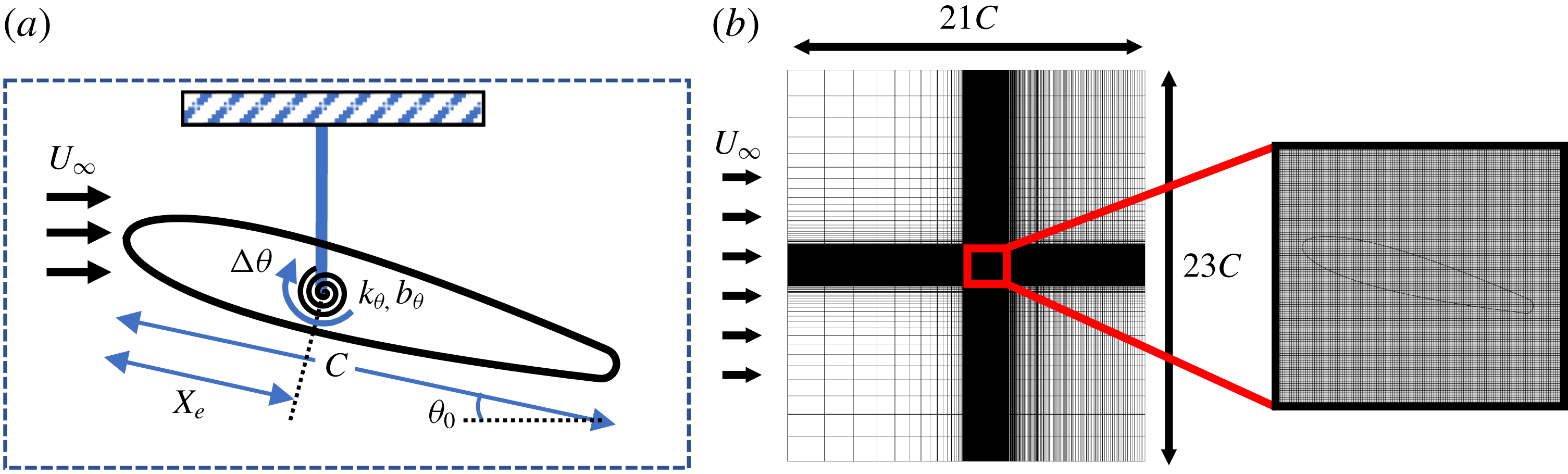
The two-dimensional computational model in the current study employs a rigid NACA0015 airfoil with a slightly rounded trailing edge, immersed in an incompressible fluid with free-stream velocity
 $U_{\infty }$
. The slight rounding of the trailing edge ensures that the flow is well resolved around it, and we have verified that this has no significant effect on the aerodynamic characteristics and forces on the airfoil. The governing incompressible Navier–Stokes equations expressed in the dimensionless form as follows:
 $$\begin{eqnarray}\frac{\unicode[STIX]{x2202}\boldsymbol{u}}{\unicode[STIX]{x2202}t}+\boldsymbol{u}\boldsymbol{\cdot }\unicode[STIX]{x1D735}\boldsymbol{u}=-\unicode[STIX]{x1D735}p+\frac{1}{Re}\unicode[STIX]{x1D6FB}^{2}u,\end{eqnarray}$$
where
 $Re=\unicode[STIX]{x1D70C}U_{\infty }C/\unicode[STIX]{x1D707}$
is the chord-based Reynolds number. The torsional elasticity of the airfoil is modelled using a linear torsional spring with spring constant
 $k$
and damping coefficient
 $b$
, attached to the rigid airfoil at a prescribed chordwise location (
 $X_{e}$
), which we refer to as the elastic axis (normalized location denoted as
 $X_{e}^{\ast }=X_{e}/C$
). The equilibrium angular position of the spring is denoted by angle
 $\unicode[STIX]{x1D703}_{0}$
. A schematic of this set-up is shown in figure 1.
(a) Schematic of the aeroelastic system used in this study; (b) computational domain and close-up of the Cartesian computational grid.

The structural system is governed by the equation for a forced spring–mass–damper oscillator. The equation is scaled by the characteristic variables used for the flow (length:
 $C$
; time:
 $c/U_{\infty }$
), and the resulting non-dimensionalized equation governing the dynamics in pitch of the airfoil is given by
 $$\begin{eqnarray}I^{\ast }\ddot{\unicode[STIX]{x1D703}}+b^{\ast }\dot{\unicode[STIX]{x1D703}}+k^{\ast }(\unicode[STIX]{x1D703}-\unicode[STIX]{x1D703}_{0})=C_{M},\end{eqnarray}$$
where
 $C_{M}=M/(0.5\unicode[STIX]{x1D70C}U_{\infty }^{2}C^{3})$
is the coefficient of aerodynamic pitching moment, and
 $I^{\ast }=2I/(\unicode[STIX]{x1D70C}C^{4})$
,
 $b^{\ast }=2b/(\unicode[STIX]{x1D70C}U_{\infty }C^{3})$
,
 $k^{\ast }=2k/(\unicode[STIX]{x1D70C}U_{\infty }^{2}C^{2})$
are the dimensionless moment of inertia, damping and spring stiffness respectively. Here,
 $C_{M}$
and
 $I^{\ast }$
are calculated with respect to
 $X_{e}^{\ast }$
. The spring stiffness is commonly expressed in terms of a reduced velocity,
 $U^{\ast }=U_{\infty }/f_{s}C$
where
 $f_{s}=(1/2\unicode[STIX]{x03C0})\sqrt{k/I}$
is the natural frequency of the spring. In essence,
 $U^{\ast }$
is a ratio of the natural time scale of the elastic system to the convective time scale of the flow. However, as we will show, the choice of fluid time scale has significant implications for the dynamics of the system.
Thus, even this highly simplified configuration has six governing parameters (
 $Re$
,
 $X_{e}^{\ast }$
,
 $I^{\ast }$
,
 $b^{\ast }$
,
 $U^{\ast }$
,
 $\unicode[STIX]{x1D703}_{0}$
) and this is indicative of the inherent complexity of this configuration. In the current study, we fix the values of
 $Re$
and
 $I^{\ast }$
to 1000 and 4.1 respectively and explore the effect of the other four parameters. The Reynolds number chosen is high enough so as to generate robust vortex shedding phenomenon, which drives flutter, but is also low enough so as to allow resolved simulations at a reasonable computational expense. The choice of the moment of inertia about the elastic axis corresponds to a solid-to-fluid density ratio of
 ${\approx}120$
. While the effect of varying
 $I^{\ast }$
in this system could be of significant engineering interest, we choose to use a fixed value throughout this study to reduce the number of independent parameters. However, it must be noted that varying
 $I^{\ast }$
is equivalent to changing the natural frequency as
 $f_{s}\sim 1/\sqrt{I^{\ast }}$
, which is an important parameter in this study.
The current study addresses structurally damped as well as undamped systems with damping being defined by
 $\unicode[STIX]{x1D701}^{\ast }=b/b_{cr}$
where
 $b_{cr}=2\sqrt{kI}$
, is the critical damping for the harmonic oscillator. For the undamped system
 $\unicode[STIX]{x1D701}^{\ast }=0$
and for the damped system we prescribe
 $\unicode[STIX]{x1D701}^{\ast }=0.15$
where this lightly damped structure enables us to understand the effect of damping without overly damping the pitch oscillations. The remaining two parameters, the elastic axis (
 $X_{e}^{\ast }$
) and the spring stiffness (
 $U^{\ast }$
), are a particular focus of the current study. For
 $X_{e}^{\ast }$
, we use three values –
 $X_{e}^{\ast }=0.50$
, 0.33 and 0.25 – and we will show that these generate very significant variations in the pitch response. The final parameter
 $U^{\ast }$
represents the spring stiffness (a larger
 $U^{\ast }$
corresponds to a softer spring) and this parameter is varied from about 2 to 13.
2.2 Numerical method
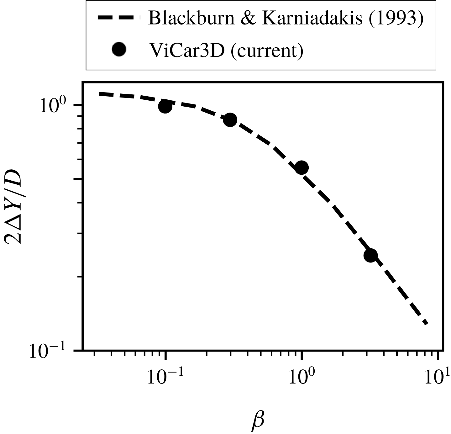
We simulate the coupled fluid–structure system using the sharp-interface immersed boundary method based solver ‘ViCar3D’ described in Mittal et al. (Reference Mittal, Dong, Bozkurttas, Najjar, Vargas and von Loebbecke2008) and Seo & Mittal (Reference Seo and Mittal2011). This allows us to preserve sharp interfaces along the surface of our geometry using a body-non-conformal Cartesian grid. This is particularly useful in fluid–structure interaction studies as it allows us to simulate a variety of shapes as well as large-amplitude motions on simple, non-adaptive Cartesian grids. In particular, this approach has the advantage of not being constrained by highly deformed grid cells or the need to periodically recompute the grid during high-amplitude motions (Mittal & Iaccarino Reference Mittal and Iaccarino2005). The fluid equations are solved using a second-order fractional-step method, and the pressure Poisson equation is solved using the geometric multigrid method. Second-order finite differences are used for all spatial derivatives, and the time integration is performed using a second-order Adams–Bashforth method. ViCar3D employs a boundary imposition scheme that is second-order accurate and consequently, models surface quantities such as pressure and shear with high fidelity (Mittal et al. Reference Mittal, Dong, Bozkurttas, Najjar, Vargas and von Loebbecke2008). ViCar3D has been validated and verified extensively for a variety of stationary and moving boundary problems in earlier papers (Ghias, Mittal & Dong Reference Ghias, Mittal and Dong2007; Mittal et al. Reference Mittal, Dong, Bozkurttas, Najjar, Vargas and von Loebbecke2008; Seo & Mittal Reference Seo and Mittal2011), as well as during the current study (see appendix B).
The fluid–structure coupling employs a loosely coupled approach wherein the flow and dynamical equation are solved sequentially. The aerodynamic forces/moments are calculated on the Lagrangian marker points on the surface of the solid body, and passed on to the solid dynamical equation (2.2). The angular velocity predicted from this equation is subsequently imposed on the marker points. The aeroelastic system is immersed in a large
 $21C\times 23C$
computational domain, where the airfoil is placed 10 chord-lengths from the downstream boundary, and the isotropic grid resolution around the solid body corresponds to approximately 125 points along the chord. The grid is stretched in all directions away from the rectangular region that surrounds the foil and the near wake resulting in a baseline grid of
 $384\times 320$
points. A Dirichlet velocity boundary condition is used at the inlet boundary of the domain, and zero-gradient Neumann conditions are specified at all other boundaries. Grid refinement studies described in appendix B confirm that the results on this grid are well converged.
For all the cases simulated here, we initialize the airfoil at its equilibrium angle
 $\unicode[STIX]{x1D703}_{0}$
, with zero initial angular velocity. The constant free-stream flow is then imposed and the dynamics allowed to evolve until the system reaches a stationary state. For the cases simulated here, it takes between
 $O(20)$
and
 $O(200)$
oscillation cycles before this stationary state is achieved. Average quantities are computed after the stationary state is reached.
3 Results
3.1 Qualitative features
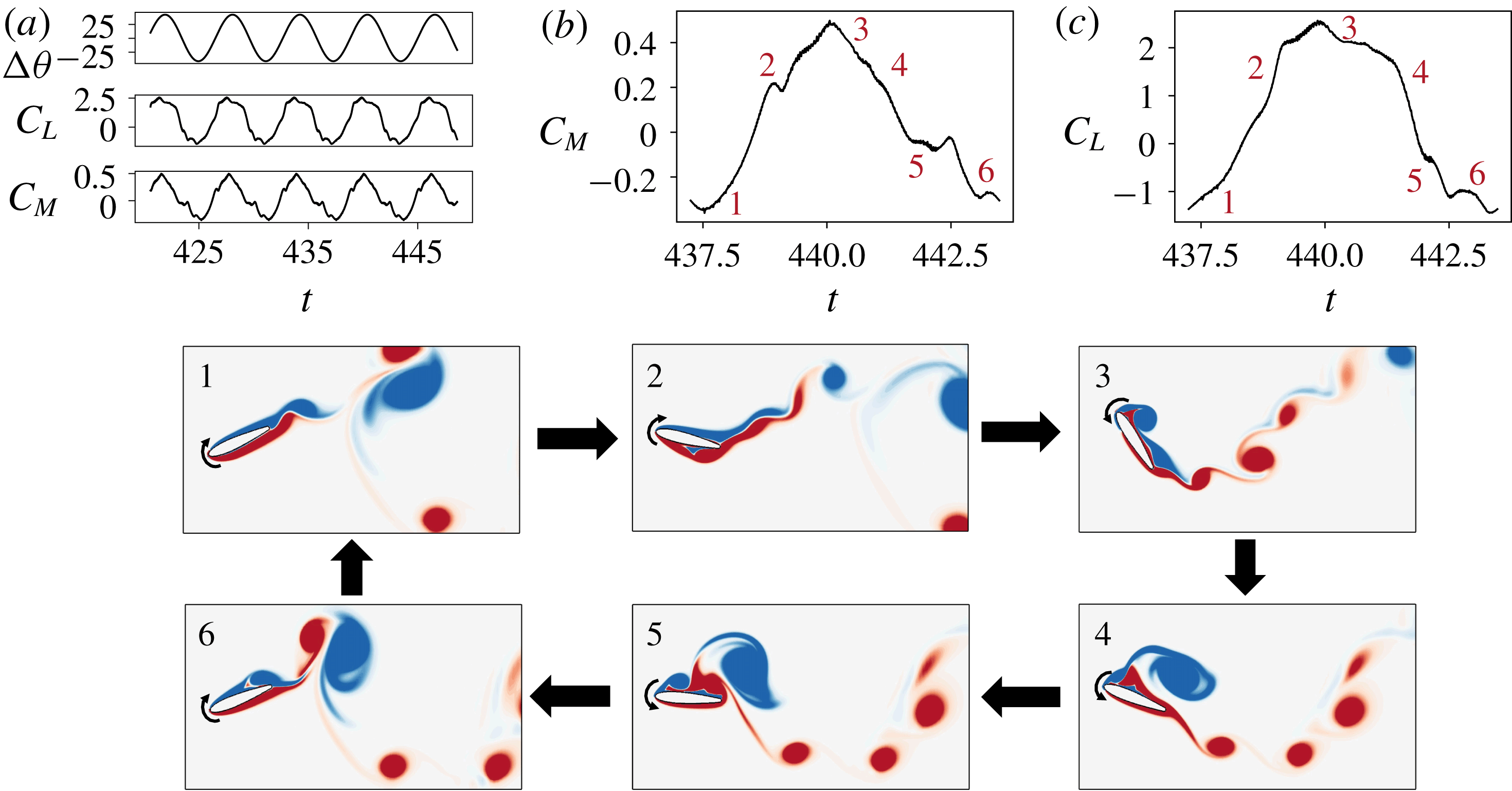
A representative case of flow-induced pitching oscillations with
 $U^{\ast }=6.6$
,
 $X_{e}^{\ast }=0.50$
,
 $\unicode[STIX]{x1D703}_{0}=15^{\circ }$
and
 $\unicode[STIX]{x1D701}=0.15$
; time series plots of (a) pitch deflection (
 $\unicode[STIX]{x0394}\unicode[STIX]{x1D703}$
), coefficient of moment (
 $C_{M}$
) and coefficient of lift (
 $C_{L}$
); (b) coefficient of moment during one cycle of oscillation (corresponding to the cycle shown in the snapshots); (c) coefficient of lift during the cycle corresponding to the snapshots; (1–6) snapshots of the flow field coloured by contours of
 $z$
-vorticity. Time is non-dimensionalized by
 $C/U_{\infty }$
.

We begin our discussion of the aeroelastic response of this system by providing an overview of one representative case for which
 $U^{\ast }=6.6$
,
 $X_{e}^{\ast }=0.5$
,
 $\unicode[STIX]{x1D701}=0.15$
and
 $\unicode[STIX]{x1D703}_{0}=15^{\circ }$
. This case develops fairly large-amplitude pitch oscillations (
 $A_{\unicode[STIX]{x1D703}}\approx 45^{\circ }$
) and serves to demonstrate the various flow structures and nonlinear interactions that drive the pitching of the airfoil. In figure 2 are snapshots of the flow over the course of one oscillation cycle. The time series for the coefficients of moment (
 $C_{M}$
) and lift (
 $C_{L}$
) corresponding to the same oscillation cycle are shown in figures 2(b) and 2(c).
As the airfoil pitches up at the start of the cycle, in figure 2(1), we see that there is initially a monotonic increase in
 $C_{M}$
and
 $C_{L}$
. This is related to the fact that the shear layer on the suction side is stabilized by the motion of the airfoil until angles of attack well past the static stall angle (which for this airfoil, at this Reynolds number, is approximately
 $20^{\circ }$
). This stabilization of the boundary layer over a pitching airfoil was also reported by Lee & Gerontakos (Reference Lee and Gerontakos2004). However, this pitch-up motion destabilizes the pressure-side boundary layer. As a result, there is a roll-up of the leading-edge shear layer on the pressure side, and a vortex convects downstream along the pressure side, as seen in figure 2(2). As this vortex moves past the trailing edge, there is a sudden drop in
 $C_{M}$
and a slight rise in
 $C_{L}$
. However, the airfoil continues to rotate on account of inertia, until it reaches its maximum pitch position. Close to the end of this motion, the LEV begins to grow, along with the shedding of a trail of smaller vortices from the trailing edge, seen in figure 2(3). A similar observation was made by Onoue & Breuer (Reference Onoue and Breuer2016), who attributed the origin of this to a Kelvin–Helmholtz-like instability in the trailing-edge shear layer. This is accompanied by a sharp loss in
 $C_{L}$
at the end of the pitch-up motion.
As the airfoil begins pitching down, there is an initial monotonic decrease in
 $C_{M}$
and
 $C_{L}$
that appears to mirror the initial stage of the pitch-up motion. We also see that the presence of the LEV over the suction surface in figure 2(4) influences the rate of this decrease. This pitch-down motion destabilizes the suction-side shear layer, and leads to the shedding of a second, smaller LEV in figure 2(5). At the same time, a trailing-edge vortex (TEV) is generated and shed, and this vortex seems to be influenced by the strong entrainment due to the LEV convecting past the trailing edge. This effect is seen in the majority of cases simulated. The simultaneous presence of this TEV and LEV near the suction side trailing edge causes a strong uptick in
 $C_{M}$
, which causes it to go over its pitch-up value. This interesting effect leads to a counter-clockwise loop in the
 $C_{M}$
hysteresis curve (not shown here), which has implications for energy-harvesting applications. Subsequently,
 $C_{M}$
continues to decrease and
 $C_{L}$
plateaus as the second LEV convects over the suction side in figure 2(6). The movement of this LEV past the trailing edge then produces a drop in
 $C_{L}$
and a brief increase in
 $C_{M}$
.
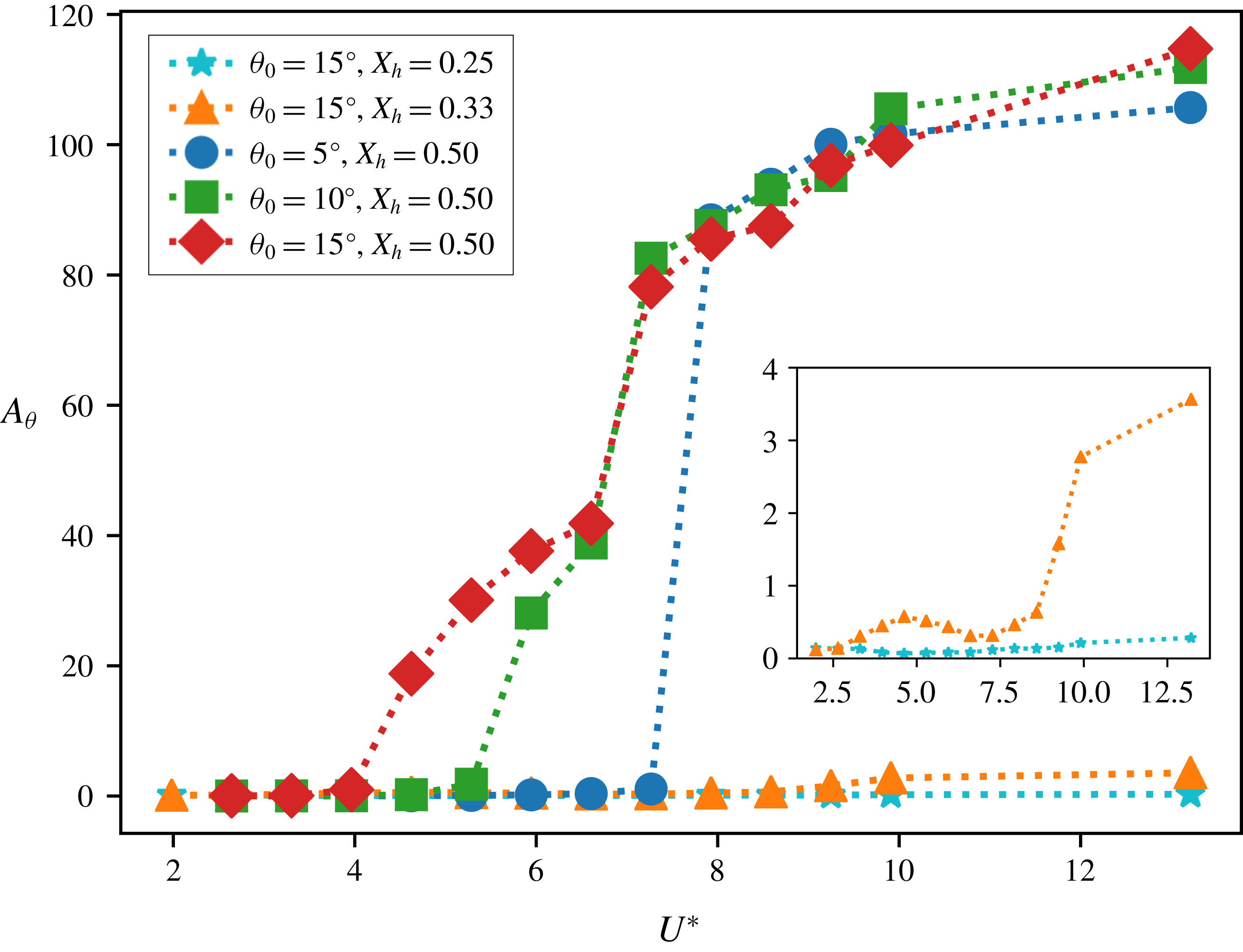
Maximum pitch deflection,
 $A_{\unicode[STIX]{x1D703}}$
, as a function of
 $U^{\ast }$
for different values of
 $\unicode[STIX]{x1D703}_{0}$
and
 $X_{e}^{\ast }$
. For all cases shown here,
 $\unicode[STIX]{x1D701}=0.15$
. The inset shows a zoom-in for
 $X_{e}^{\ast }=0.25$
and
 $X_{e}^{\ast }=0.33$
.

This representative case shows that the airfoil experiences strongly nonlinear loading over the course of an oscillation cycle. The occurrence of limit-cycle oscillations, which we see in spite of a linear structural model, is only possible in the presence of such nonlinearities in the system. Hence, this supports the notion that large-scale flow separation is the primary cause of limit-cycle oscillations in this system. Further, there is a complex interaction between the leading- and trailing-edge shear layers, as well as the generation and shedding of multiple LEVs. The timing and position of these flow structures play crucial roles in the dynamics of pitch oscillations, and this analysis of some representative flow interactions forms a starting point of our discussion.
3.2 Effect of key parameters on flutter response
The overall effect of spring stiffness (
 $U^{\ast }$
), equilibrium angle of attack and elastic-axis location on the flutter amplitude is discussed in this section. In figure 3, we show the maximum stationary-state pitch deflection from the equilibrium (denoted as
 $A_{\unicode[STIX]{x1D703}}$
), as a function of
 $U^{\ast }$
for the case with non-zero structural damping. This is plotted for three different equilibrium pitch angles,
 $\unicode[STIX]{x1D703}_{0}=5^{\circ }$
,
 $10^{\circ }$
,
 $15^{\circ }$
, and three different locations of the elastic axis,
 $X_{e}^{\ast }=0.25$
, 0.33, 0.50. It is immediately clear that this system can show very large pitch deflections, going as high as
 $100^{\circ }$
, for the case of
 $X_{e}^{\ast }=0.50$
. However, the pitch deflections for
 $X_{e}^{\ast }=0.25$
and
 $0.33$
are very small for the same range of
 $U^{\ast }$
. Further, while the response for
 $X_{e}^{\ast }=0.50$
increases monotonically with
 $U^{\ast }$
, the response for
 $X_{e}^{\ast }=0.33$
shows a non-monotonic trend (shown in the inset). These observations suggest that the amplitude response of this system is very sensitive to the location of the elastic axis, and this issue is investigated further in §§ 4 and 3.5. The lack of response at
 $X_{e}^{\ast }=0.25$
is not surprising since the aerodynamic centre of most airfoils is in the vicinity of 25 % chord (Abbott & Von Doenhoff Reference Abbott and Von Doenhoff1959) and placing the elastic axis at or near this location should diminish pitch instability.
We now focus on the large-amplitude flutter observed for the
 $X_{e}^{\ast }=0.50$
cases. We see that the onset of these large amplitude oscillations occurs at a different (critical)
 $U^{\ast }$
(referred to as
 $U_{c}^{\ast }$
) for each value of
 $\unicode[STIX]{x1D703}_{0}$
. Lower
 $\unicode[STIX]{x1D703}_{0}$
requires softer springs (or higher
 $U^{\ast }$
) in order to initiate deflections. Interestingly,
 $A_{\unicode[STIX]{x1D703}}$
for different values of
 $\unicode[STIX]{x1D703}_{0}$
approach each other for very large pitch deflections indicating that the system loses memory of the equilibrium condition for very soft springs. As a result of this, and the fact that the bifurcation is delayed for lower
 $\unicode[STIX]{x1D703}_{0}$
, the onset of large-amplitude oscillations is more abrupt as we go to lower
 $\unicode[STIX]{x1D703}_{0}$
, i.e. the curve for
 $\unicode[STIX]{x1D703}_{0}=5^{\circ }$
has a larger slope than that for
 $\unicode[STIX]{x1D703}_{0}=10^{\circ }$
. This points to the possibility of a bifurcation that has an increasingly subcritical nature as
 $\unicode[STIX]{x1D703}_{0}$
is reduced. This is in agreement with Dimitriadis & Li (Reference Dimitriadis and Li2009) and Onoue et al. (Reference Onoue, Song, Strom and Breuer2015) who observed a subcritical bifurcation for
 $\unicode[STIX]{x1D703}_{0}=0^{\circ }$
. It must be noted here that unlike the case of
 $\unicode[STIX]{x1D703}_{0}=0^{\circ }$
, our system shows small, but non-zero, values of
 $A_{\unicode[STIX]{x1D703}}$
even for very low
 $U^{\ast }$
. These oscillations are associated with the oscillatory pitch moments induced by Kármán vortex shedding. However, we will show the presence of subcritical behaviour even in the case of
 $\unicode[STIX]{x1D703}_{0}=15^{\circ }$
later in this paper.
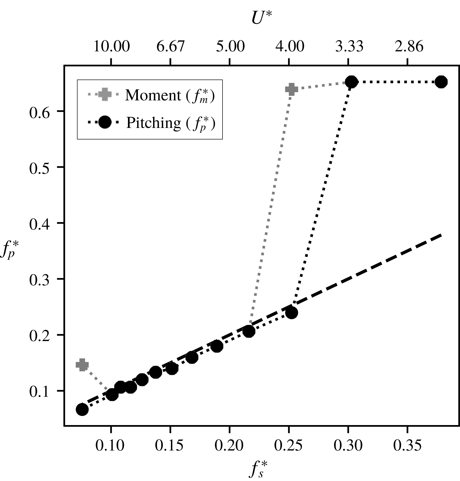
3.3 Frequency response
Pitch and moment frequency response as a function of
 $U^{\ast }$
for
 $\unicode[STIX]{x1D703}_{0}=15^{\circ }$
,
 $X_{e}^{\ast }=0.50$
and
 $\unicode[STIX]{x1D701}=0.15$
. The dashed line shows the natural frequency.

In the previous section, we showed that the system loses memory of the equilibrium condition (
 $\unicode[STIX]{x1D703}_{0}$
) for large flutter amplitudes. Considering this, we will conduct a detailed analysis for one case, namely
 $\unicode[STIX]{x1D703}_{0}=15^{\circ }$
. In figure 4 we show the pitch oscillation frequency (
 $f_{p}^{\ast }=f_{p}C/U$
) compared with the frequency of moment oscillations (
 $f_{m}^{\ast }=f_{m}C/U$
) for the structurally damped case with
 $\unicode[STIX]{x1D703}_{0}=15^{\circ }$
and
 $\unicode[STIX]{x1D701}=0.15$
. This is plotted with respect to the dimensionless natural frequency
 $f_{s}^{\ast }$
as well as
 $U^{\ast }=1/f_{s}^{\ast }$
. The dashed line in figure 4 denotes the synchronization condition, i.e. the condition where the pitch frequency equals the natural frequency of the system. We see that for low (high) values of
 $U^{\ast }$
(
 $f_{s}^{\ast }$
), the pitch as well as moment oscillations occur at a constant, high frequency. On increasing
 $U^{\ast }$
, there is a sudden drop in frequency which corresponds to the same
 $U^{\ast }$
value at which the bifurcation to large-amplitude pitch oscillation occurs – following which, the pitch oscillations synchronize with the natural frequency for higher (lower) values of
 $U^{\ast }$
(
 $f_{s}^{\ast }$
). Hence, there are three distinct frequency response regimes that occur for increasing (decreasing)
 $U^{\ast }$
(
 $f_{s}^{\ast }$
): constant, high-frequency pitch and moment, followed by the moment de-tuning from the pitch at the bifurcation point and finally the moment and pitch oscillations synchronizing with the natural frequency of the system.
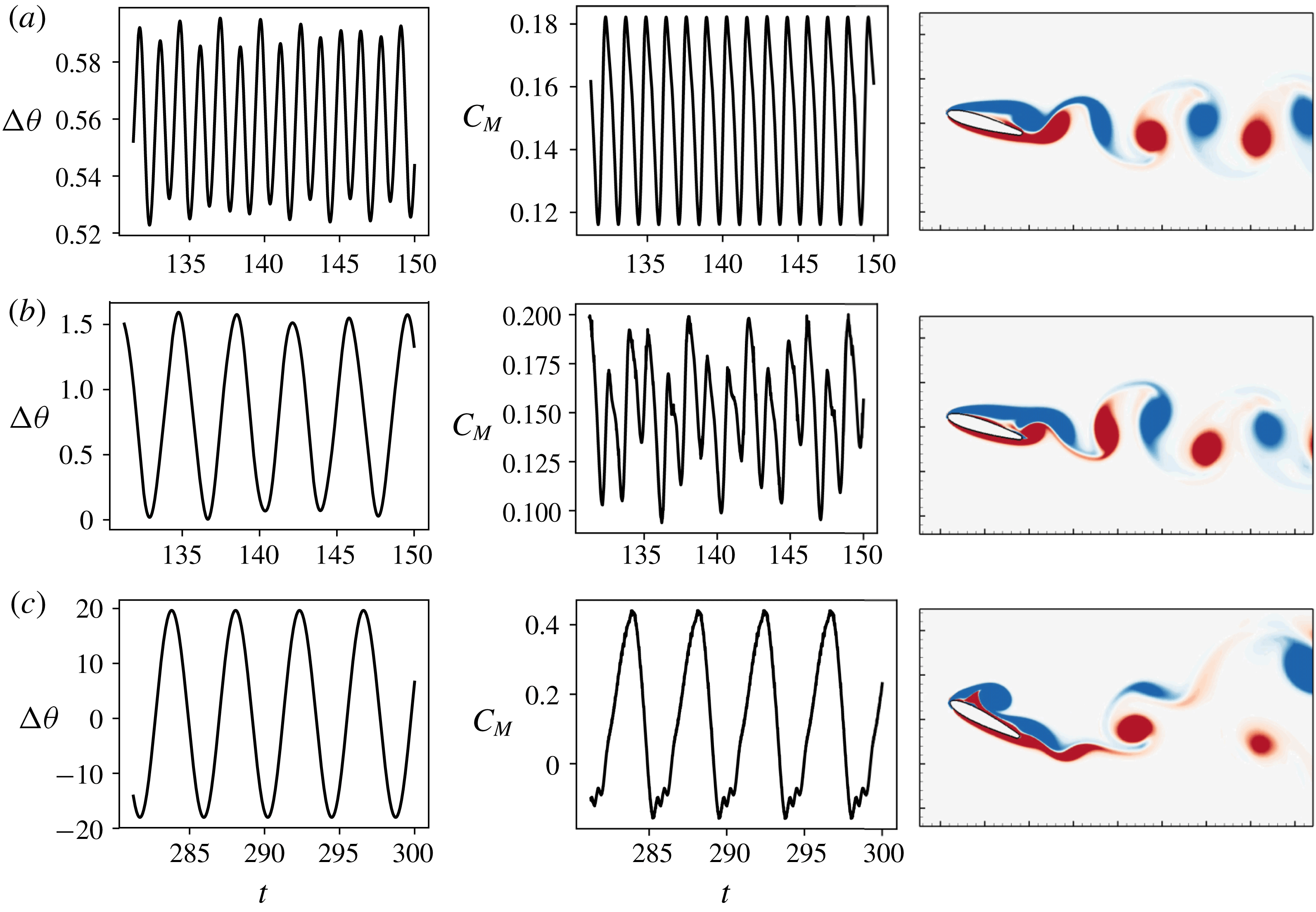
Pitch amplitude time series, (
 $\unicode[STIX]{x0394}\unicode[STIX]{x1D703}$
), coefficient of moment (
 $C_{M}$
) and a snapshot of vorticity contours for three regimes of response close to
 $U_{c}^{\ast }$
; (a)
 $U^{\ast }=3.3$
; (b)
 $U^{\ast }=4.0$
; (c)
 $U^{\ast }=4.6$
.

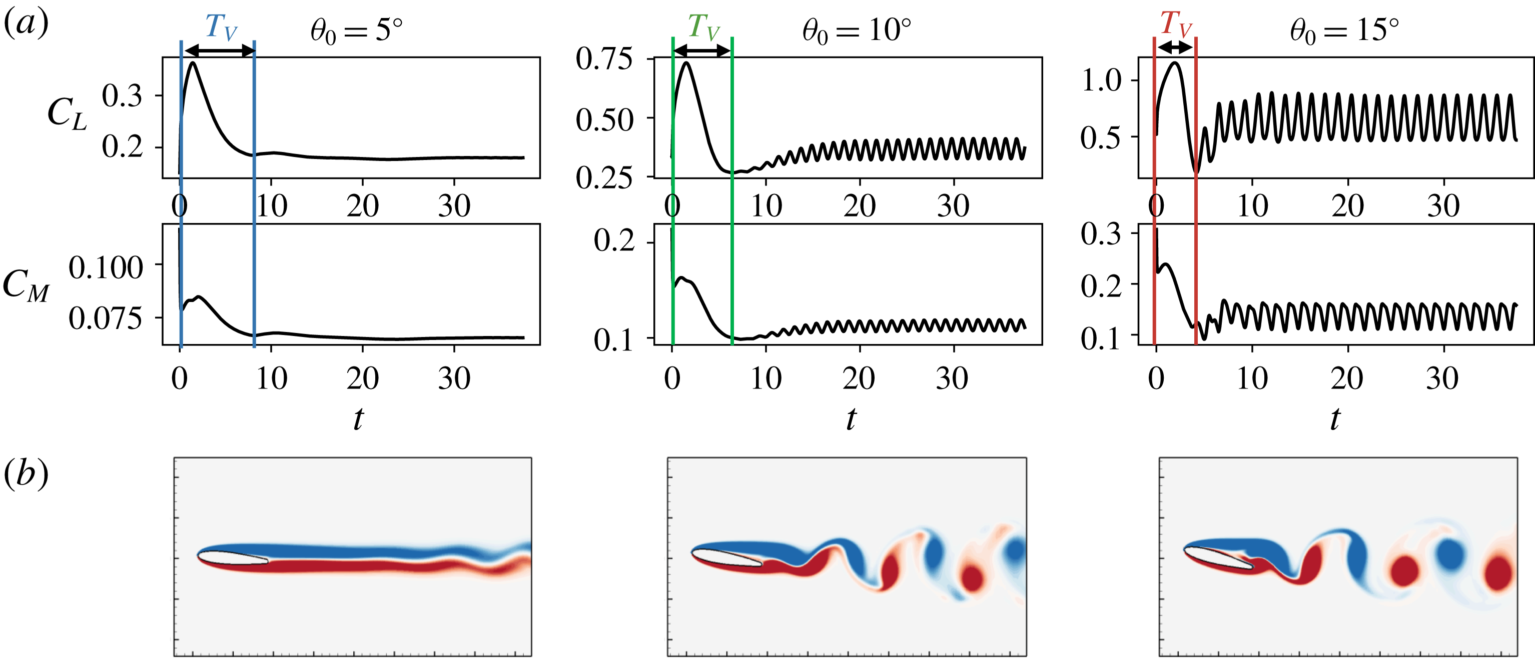
Time series of
 $C_{L}$
and
 $C_{M}$
for static airfoils at
 $\unicode[STIX]{x1D703}_{0}=5^{\circ },10^{\circ },15^{\circ }$
. (b) An instantaneous snapshot of the flow after reaching stationary state for each case, coloured by vorticity contours. Also indicated is
 $T_{v}$
, which represents the time scale of the initial transient. Note: the flow snapshots do not show the entire computational domain, which extends approximately
 $5C$
beyond the edge of the figure.

It is instructive to examine the flow quantities during these distinct regimes to understand how the flow drives the dynamics of flutter, and vice versa. In figure 5 we show plots of the pitch and moment time series, along with a snapshot of the flow, for three representative cases very close to the bifurcation point. For
 $U^{\ast }=3.3$
, which corresponds to the pre-onset regime, we see that the response amplitude is very small (
 $A_{\unicode[STIX]{x1D703}}<1^{\circ }$
), the frequency is high and the pitch moment oscillates at a similar high frequency. Due to the small amplitude of oscillation, it makes sense to compare this with the behaviour of a static airfoil and we see that the response frequency is in fact very close to the vortex shedding frequency of a static airfoil at
 $\unicode[STIX]{x1D703}_{0}=15^{\circ }$
(
 $f^{\ast }=0.71$
; see time series in figure 6). From the flow field it is clear that this regime corresponds to a Kármán vortex shedding mode, much like the wake due to separated slow around a stationary bluff body. In fact, the dimensionless frequency in this regime, when calculated using the projected frontal length as the length scale, is
 $f^{\ast }\approx 0.17$
, which is very close to the frequency of Kármán shedding in bluff body wakes. In this regime, the coupling between the flow and airfoil pitching is effectively one way, with the vortex shedding driving the pitching, but the pitching having virtually no effect on the vortex shedding.
In contrast, the flow field for
 $U^{\ast }=4.6$
, which corresponds to the post-bifurcation regime where the pitch response occurs at the natural frequency of the system, shows a very different character with the presence of a strong dynamic stall vortex generated at the leading edge. This is also apparent in the time series of the moment coefficient, where the peak of the oscillation is accompanied by an abrupt drop in forcing. This drop in forcing has been observed by numerous studies as a hallmark of dynamic stall. In this regime, large (
 $20^{\circ }$
) amplitude pitch oscillations occur at the natural frequency, which in turn force the generation and shedding of the stall vortex to occur at this frequency.
For the intermediate case of
 $U^{\ast }=4.0$
, which corresponds to the regime close to the bifurcation, the pitch time series shows low-frequency oscillations at to the natural frequency. The moment time series however seems to have frequency components corresponding to the vortex shedding as well airfoil pitching time scale. This is qualitatively seen in the flow field too, where the wake has the appearance of a slightly undulating or distorted Kármán wake. Hence this is a transitional regime that occurs between the pre- and post-bifurcation regimes.
This regime of oscillation in fact agrees well with the observation of Poirel et al. (Reference Poirel, Harris and Benaissa2008) who investigated flutter oscillations in this range of amplitudes. They too observed low-frequency pitch oscillations which showed no signature of the high-frequency Kármán shedding occurring in the wake. Further, this low-frequency content is absent in the pre-bifurcation (or static) regime forcing response. The triggering of low-frequency oscillations in the absence of low-frequency forcing suggests that the flutter is not a result of an external periodic forcing, and is in fact self-sustained.
3.4 Critical reduced velocity
An obvious and important question raised by figure 3 is – why does the critical
 $U^{\ast }$
depend on
 $\unicode[STIX]{x1D703}_{0}$
?
 $U^{\ast }$
represents a ratio the time scale of the pitch oscillation to a time scale for the flow. With regard to the pitch time scale, it is clear from the previous subsection that in the post-critical regime, the time scale for the pitch oscillations does coincide with the natural time scale of the elastic system. Turning next to the flow time scale in
 $U^{\ast }$
we note that in most studies (including the current), the time scale for the flow is assumed to be the convective time scale of the flow over the body, i.e.
 $C/U_{\infty }$
. However, a more appropriate flow time scale is one that is associated with the mechanism that triggers the flutter instability. In the well-studied case of flow-induced vibrations of circular cylinders, it is known that the trigger for the cylinder vibrations is Kármán vortex shedding (Williamson & Govardhan Reference Williamson and Govardhan2004). The appropriate time scale for determining the onset of these vibrations is therefore the vortex shedding time scale (
 $T_{v}$
), which is approximately
 $5D/U_{\infty }$
. Thus, a reformulation of the reduced velocity as the ratio of the natural time scale of the elastic structure and the vortex shedding time scale as
 $U_{v}^{\ast }=(1/f_{s})/(5D/U_{\infty })$
leads to the condition that vibrations are initiated when
 $U_{v}^{\ast }$
approaches and exceeds unity. The identification of a similar scaling for the airfoil flutter observed in the current study, is the focus of the rest of this section.
Since we are concerned here with the onset of flutter, flow past a static airfoil should provide insights regarding the triggering mechanism. With this in mind we perform a set of simulations of flow over static airfoils at
 $Re=1000$
with the angle of attack set to
 $\unicode[STIX]{x1D703}_{0}$
for each case. The system is held at this angle of attack and the flow proceeds through the transient to its final stationary state. In figure 6 we show time-series plots of the lift and moment generated by these cases and also the instantaneous contours of spanwise vorticity for each case. The lowest
 $\unicode[STIX]{x1D703}_{0}$
exhibits weak vortex shedding beyond the near wake whereas the other two cases exhibit separation of the boundary layer from the suction surface of the airfoil as well as vortex shedding in the wake with a topology that is quite similar to Kármán shedding. The frequency corresponding to this vortex shedding is
 $0.81U_{\infty }/C$
and
 $0.71U_{\infty }/C$
for
 $\unicode[STIX]{x1D703}_{0}=10^{\circ }$
and
 $15^{\circ }$
, respectively. However, these are higher than the frequency corresponding to the system at the onset of flutter and can therefore not be the triggering mechanisms for post-onset flutter oscillations. In fact, the static
 $\unicode[STIX]{x1D703}_{0}=5^{\circ }$
case does not exhibit vortex shedding but still undergoes a bifurcation to large-scale flutter, further confirming that wake vortex shedding is not the trigger for the bifurcation. This agrees with the observations of Poirel et al. (Reference Poirel, Harris and Benaissa2008).
Figure 6 however, suggests an alternative time scale for the onset and sustenance of flutter, which manifests itself during the initial transient over the static airfoil. The initial transient in the current simulations represents the initial growth, development and saturation of the vorticity layer over the two surfaces of the airfoil and this transient is associated with a distinct, large-magnitude peak in the lift and moment, with a well-defined time scale. This time scale is associated with an intrinsic time scale for the separated shear layer, which is the key driver for flutter. Based on this, we hypothesize that the time scale that corresponds to the relaxation time of a perturbation in the separated shear layer would be the appropriate time scale for determining the onset of flutter.
It is possible to estimate this time scale for the current configuration by using a system-identification approach. This is done by providing a small perturbation to the angle of attack of an airfoil which is held stationary before and after the perturbation, and estimating the time it takes for the resulting pitching moment on the airfoil to relax back to the unperturbed state. In this study, the pitch perturbation takes the form
 $\unicode[STIX]{x1D703}_{p}(t)=A_{p}[1-\cos \{2\unicode[STIX]{x03C0}(t-t_{0})/\unicode[STIX]{x1D70F}_{p}\}]$
, where
 $A_{p}$
is the amplitude of the perturbation,
 $t_{0}$
is the time at which the perturbation is applied and
 $\unicode[STIX]{x1D70F}_{p}$
is the duration of the perturbation. In the current case,
 $\unicode[STIX]{x1D70F}_{p}$
is chosen equal to
 $C/U_{\infty }$
, which is much smaller than the observed time scales of the initial transient and resembles a ‘delta’ perturbation. A qualitative representation of this perturbation is shown for the case of
 $\unicode[STIX]{x1D703}_{0}=5^{\circ }$
in figure 7. We then compute the perturbation in the pitching moment by subtracting the unperturbed moment coefficient (which we refer to as
 $C_{M_{0}}$
) from the pitching moment measured following the perturbation. For simplicity, these signals are filtered to remove vortex shedding oscillations. The required time scale (
 $T_{v}$
) is then estimated as the time taken by the energy of this perturbation to attain 5 % of its peak value. The above procedure is performed for
 $\unicode[STIX]{x1D703}_{0}=5^{\circ },10^{\circ },15^{\circ }$
using perturbations at various phases of the natural vortex shedding. Furthermore, the following magnitudes of perturbation,
 $A_{p}$
are employed:
 $0.1^{\circ },0.125^{\circ },0.25^{\circ }$
for
 $\unicode[STIX]{x1D703}_{0}=5^{\circ }$
;
 $0.125^{\circ },0.25^{\circ },0.5^{\circ }$
for
 $\unicode[STIX]{x1D703}_{0}=10^{\circ }$
; and
 $1.5^{\circ },2^{\circ },2.5^{\circ }$
for
 $\unicode[STIX]{x1D703}_{0}=15^{\circ }$
.
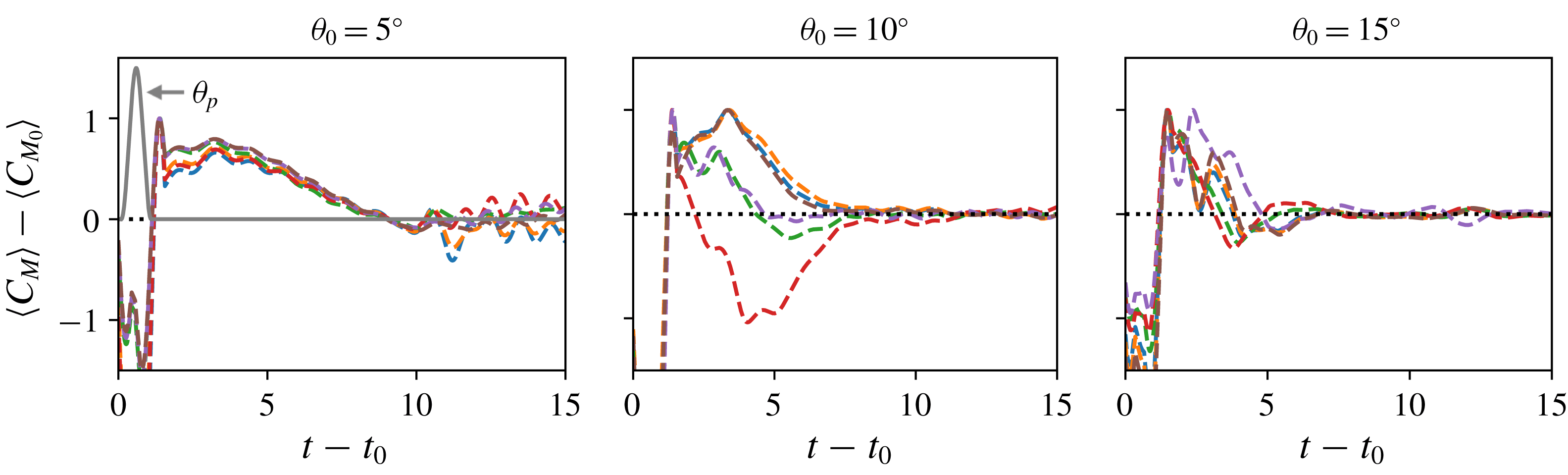
Relaxation of perturbed
 $C_{M}$
as a result of small perturbations in angle of attack for static airfoils at
 $\unicode[STIX]{x1D703}_{0}=5^{\circ },10^{\circ },15^{\circ }$
.
 $\langle C_{M}\rangle$
and
 $\langle C_{M_{0}}\rangle$
are filtered moment coefficients of perturbed and unperturbed cases respectively. The different curves in each plot correspond to different values of
 $A_{p}$
and
 $t_{0}$
. Also shown qualitatively for the case of
 $\unicode[STIX]{x1D703}_{0}=5^{\circ }$
is the pitch angle perturbation,
 $\unicode[STIX]{x1D703}_{p}$
. Time in these plots is non-dimensionalized by
 $C/U_{\infty }$
.

Figure 7 shows the time variation in the moment coefficient for these various cases at each
 $\unicode[STIX]{x1D703}_{0}$
. It is observed that, depending on the phase of vortex shedding at which the perturbation is applied, the perturbed moment coefficient can be positive or negative. However, all the perturbation with different phases and magnitudes result in a consistent relaxation time scale for each
 $\unicode[STIX]{x1D703}_{0}$
. This time scale is estimated to be
 $T_{v}\approx 7.0$
, 5.1 and 4.0 for
 $\unicode[STIX]{x1D703}_{0}=5^{\circ }$
,
 $10^{\circ }$
and
 $15^{\circ }$
, respectively. It is noted that the time scale reduces with increasing angle of attack, a trend that was also observed for the initial transient in figure 6.
We now use
 $T_{v}$
to define a new reduced velocity
 $U_{v}^{\ast }=1/(f_{s}T_{v})$
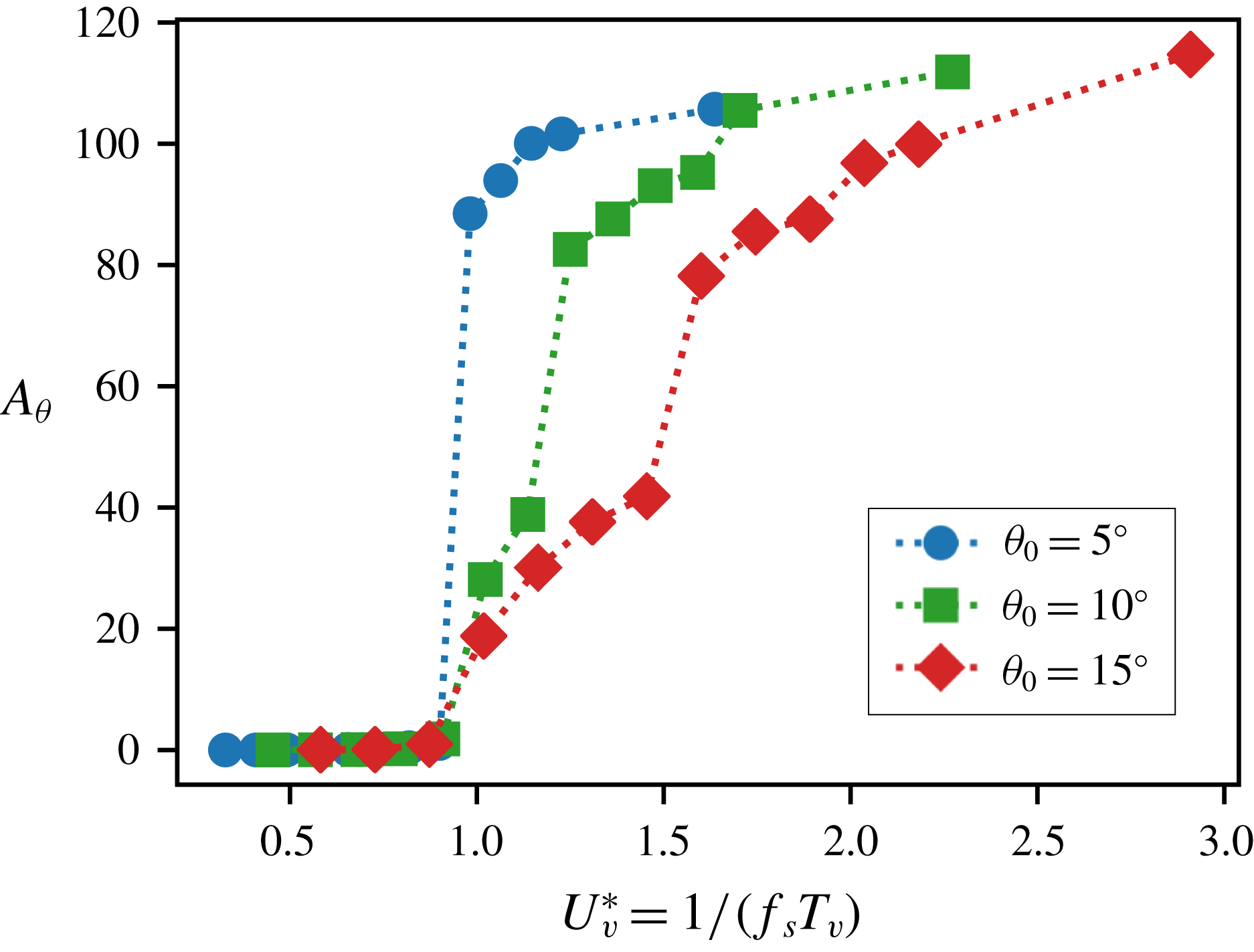
. In figure 8 we replot the maximum pitch deflection (which was initially shown in figure 3) versus
 $U_{v}^{\ast }$
and we find not only that the bifurcation points for the three cases collapse to nearly the same value, but also that this critical value is slightly above unity. This strongly suggests that
 $T_{v}$
is the correct flow time scale for this problem and in an analogue of the flow-induced vibration of a circular cylinder,
 $U_{v}^{\ast }\gtrapprox 1$
is the simple condition for the generation of large-scale flutter, at least for the low Reynolds numbers investigated here.
Maximum pitch deflection versus
 $U_{v}^{\ast }=1/(f_{s}T_{v})$
for
 $\unicode[STIX]{x1D703}_{0}=5^{\circ },10^{\circ },15^{\circ }$
. Here
 $\unicode[STIX]{x1D701}=0.15$
and
 $X_{e}^{\ast }=0.50$
.

The
 $U_{v}^{\ast }\gtrapprox 1$
condition for flutter also provides a phenomenological basis for the onset of flutter. During the pre-bifurcation regime, where the structural stiffness is higher than the critical value, the natural time scale is smaller than the flow time scale. In this condition, the time variation in pitching moment due to a perturbation in pitch does not have sufficient time to grow before the spring forces the airfoil back towards the equilibrium position. Thus, the interaction between the pitching motion and the pitching moment is not constructive and the system is not able to extract energy from the flow to sustain the oscillation. For
 $U_{v}^{\ast }>1$
, the natural time scale exceeds the flow time scale and the growth in the pitching moment associated with a pitch perturbation can now be accommodated by the spring. This constructive interaction between pitch and pitching moment is able to extract energy from the flow during a pitch perturbation, leading to growth of the pitch instability. In a later section, we will revisit this idea of energy extraction and its influence on driving aeroelastic flutter.
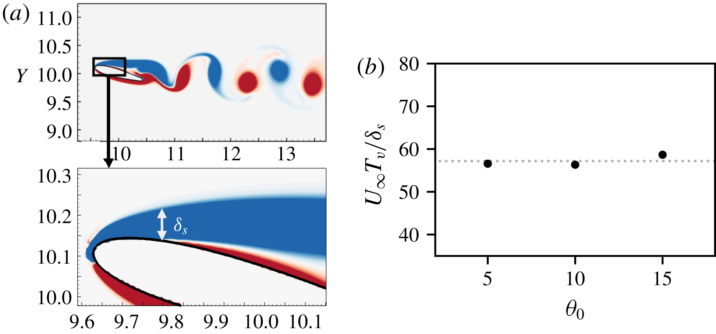
(a) Qualitative representation of boundary layer thickness at separation point for
 $\unicode[STIX]{x1D703}_{0}=15^{\circ }$
; (b) scaling of the shear-layer time scale (
 $T_{v}$
) with estimated boundary layer thickness (
 $\unicode[STIX]{x1D6FF}_{s}$
) for
 $\unicode[STIX]{x1D703}_{0}=5^{\circ },10^{\circ },15^{\circ }$
.

The physical underpinning of the dependence of
 $T_{v}$
on the angle of attack is the final question regarding the onset of flutter. In particular, why does
 $T_{v}$
decrease with increasing angle of attack? We base our analysis on the notion that
 $T_{v}$
is related to the inherent instability of the shear layer that separates from the suction surface of the airfoil, and the natural time scale of a shear layer that separates from a surface scales with the thickness of the shear layer at the point of separation. As the angle of attack is increased, the separation point moves upstream where the attached boundary layer is thinner, and therefore the shear-layer thickness at the point of separation decreases with increasing angle of attack. We have estimated the boundary layer thickness (denoted by
 $\unicode[STIX]{x1D6FF}_{s}$
) at the point of separation for the static airfoil at the three angles of attack. This is shown qualitatively for
 $\unicode[STIX]{x1D703}_{0}=15^{\circ }$
in figure 9(a). In figure 9(b) we plot the ratio of the shear-layer time scale and boundary layer thickness, non-dimensionalized by
 $U_{\infty }$
for the three angles of attack studied here. This dimensionless number represents a relaxation time scale associated with the shear layer and the plot indicates that
 $\unicode[STIX]{x1D6FF}_{s}$
and
 $T_{v}$
have an approximately constant scaling with angle of attack. This supports our hypothesis that the reduction of
 $T_{v}$
with angle of attack is related to the shear-layer instability, which is in turn governed by its thickness at the point of separation.
3.5 Structural damping and location of elastic axis
In this section, we describe the effects of structural damping as well as the location of the elastic axis on flutter. In previous sections, we have described the response of the system with
 $b^{\ast }=0.15b_{cr}^{\ast }$
and in this section, we compare these previous cases with the corresponding cases with zero damping. Further, we will make this comparison for two different locations of the elastic axis:
 $X_{e}^{\ast }=0.50$
and 0.33. The location of the elastic axis with respect to the centre of pressure is critical in determining the aeroelastic pitch stability of an airfoil. A centre of pressure upstream of the elastic axis leads to an unstable configuration that promotes the pitching instability, and vice versa. In the context of pitching airfoils, there is the added consideration of the timing of leading-edge vortices convecting past the elastic axis. Each such vortex induces a pitching moment on the airfoil and the direction of this moment changes as the vortex convects past the elastic axis. This could potentially lead to nonlinear and non-monotonic behaviour noted in § 3.2.
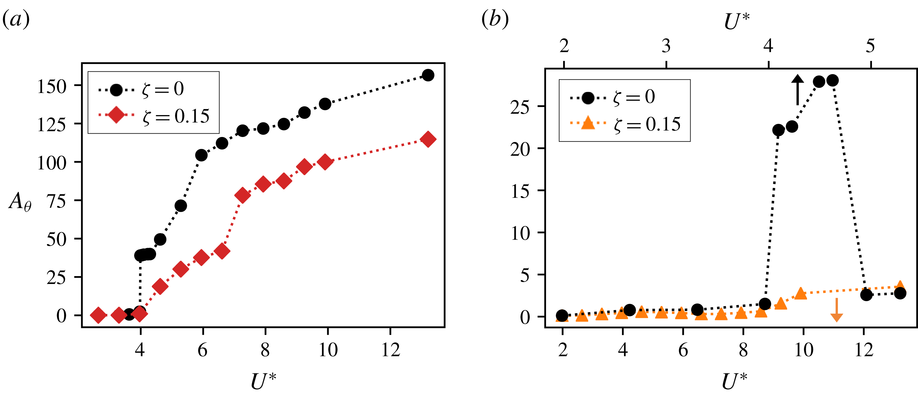
Effect of structural damping,
 $\unicode[STIX]{x1D701}$
, on maximum pitch deflection for
 $\unicode[STIX]{x1D703}_{0}=15^{\circ }$
. This is shown for two different locations of the elastic axis, (a)
 $X_{e}^{\ast }=0.50$
; (b)
 $X_{e}^{\ast }=0.33$
. Note: range of
 $U^{\ast }$
is different for each value of
 $\unicode[STIX]{x1D701}$
in the case of
 $X_{e}^{\ast }=0.33$
.

In figures 10(a) and 10(b) we plot the maximum pitch deflection,
 $A_{\unicode[STIX]{x1D703}}$
, with and without structural damping, as a function of
 $U^{\ast }$
, for two different locations of the elastic axis and for
 $\unicode[STIX]{x1D703}_{0}=15^{\circ }$
. For
 $X_{e}^{\ast }=0.50$
, we see that the overall trend of
 $A_{\unicode[STIX]{x1D703}}$
does not change significantly with damping. However, as expected, the undamped case shows a much larger amplitude of oscillations. We also see that the bifurcation to large-amplitude oscillations is very abrupt for
 $\unicode[STIX]{x1D701}^{\ast }=0.0$
, indicating a subcritical bifurcation. This agrees with the classical understanding of dynamical systems where the loss of a low-order damping term leads to a subcritical bifurcation (Strogatz Reference Strogatz2018). However, the stabilizing influence of higher-order nonlinearities (from the flow, in this case) prevents the system from diverging, and hence causes limit-cycle oscillations.
As noted previously, the amplitude response for
 $X_{e}^{\ast }=0.33$
exhibits significantly smaller oscillations, but a non-monotonic behaviour as the hinge location is moved upstream. Figure 10(b) shows that this non-monotonic behaviour of
 $A_{\unicode[STIX]{x1D703}}$
is much more apparent in the absence of structural damping, where we observe a very large and abrupt jump in flutter amplitude with
 $U^{\ast }$
. However, further increase in
 $U^{\ast }$
results in a large drop in the flutter amplitude. These types of non-monotonic responses have been studied extensively in flow-induced vibration of bluff bodies (Williamson & Govardhan Reference Williamson and Govardhan2008) but are quite unexplored for airfoil flutter.
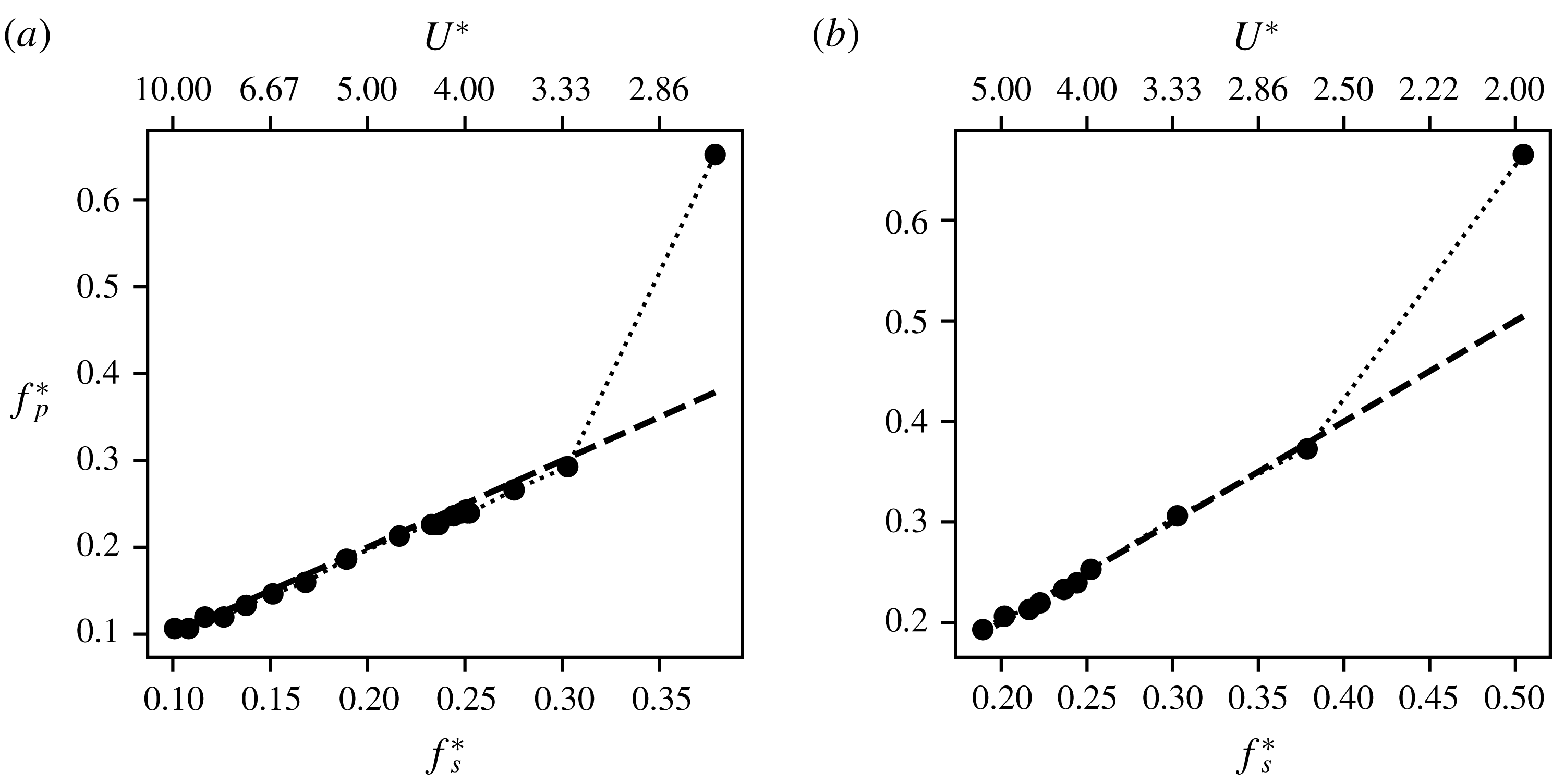
Pitching frequency response of undamped oscillations (
 $\unicode[STIX]{x1D701}=0.0$
) for
 $\unicode[STIX]{x1D703}_{0}=15^{\circ }$
and two different locations of the elastic axis, (a)
 $X_{e}^{\ast }=0.50$
; (b)
 $X_{e}^{\ast }=0.33$
. The dashed line shows the natural frequency of the system.

Figure 11 shows the frequency response of the undamped system for
 $X_{e}^{\ast }=0.50$
and 0.33 and it is clear that these cases show the same response regimes that were seen before – a high-frequency Kármán shedding mode, followed by oscillations at the natural frequency for increasing
 $U^{\ast }$
. Further, this synchronization happens close to the critical
 $U^{\ast }$
. Hence the frequency selection in this system follows a mechanism that is similar to that outlined previously, where the competition of time scales determines the response frequency. However, the amplitude response warrants further investigation.
4 Flutter analysis based on energy maps
4.1 Energy maps
Our analysis in the preceding sections indicates a need to better understand the amplitude response of the flow-induced pitching airfoil for a set of given system parameters. We were able to demonstrate the mechanism governing the onset and frequency of oscillation as a competition of time scales. However, the variations in amplitude with
 $U^{\ast }$
and
 $X_{e}^{\ast }$
are complex and non-intuitive. Here, we propose the use of ‘energy maps’ to gain an understanding of the complex amplitude response of the system. For an airfoil undergoing sinusoidal pitching oscillations in a free stream, we can derive (see appendix A) the following equation for the growth of the amplitude over one cycle
 $$\begin{eqnarray}A_{\unicode[STIX]{x1D703}}(t_{n}+T)-A_{\unicode[STIX]{x1D703}}(t_{n})=\frac{E^{\ast }}{k^{\ast }\bar{A}_{\unicode[STIX]{x1D703}}},\end{eqnarray}$$
where
 $\bar{A}_{\unicode[STIX]{x1D703}}$
is the average amplitude over a cycle. In the above equation
 $E^{\ast }=E_{f}^{\ast }-E_{d}^{\ast }$
, where
 $E_{f}^{\ast }$
is the energy extracted by the airfoil from the free stream over one oscillation cycle and
 $E_{d}^{\ast }$
is the energy lost to structural damping;
 $E_{f}^{\ast }$
is given by
 $$\begin{eqnarray}E_{f}^{\ast }=\int _{t_{n}}^{t_{n}+T}C_{M}\dot{\unicode[STIX]{x1D703}}\,\text{d}t,\end{eqnarray}$$
where
 $\dot{\unicode[STIX]{x1D703}}$
is the angular velocity and
 $T$
is the period of oscillation.
In the case of purely sinusoidal oscillations where
 $\dot{\unicode[STIX]{x1D703}}=\dot{\unicode[STIX]{x1D6E9}}\sin (2\unicode[STIX]{x03C0}t/T)$
and
 $C_{M}=K\sin (2\unicode[STIX]{x03C0}t/T+\unicode[STIX]{x1D719})$
, the energy transfer is given by
 $E_{f}^{\ast }=(1/2)\dot{\unicode[STIX]{x1D6E9}}KT\cos \unicode[STIX]{x1D719}$
and this simple model shows that the sign of energy extraction, which determines whether the airfoil extracts energy from the flow, is governed by the phase difference between the pitch velocity and the pitch moment. The physical interpretation of this phase difference, in the context of flow-induced oscillations, is related to the timing between the pitching and the resulting response of the flow. In § 3.3, our description of the mechanism determining the frequency response showed that this timing determines the critical
 $U^{\ast }$
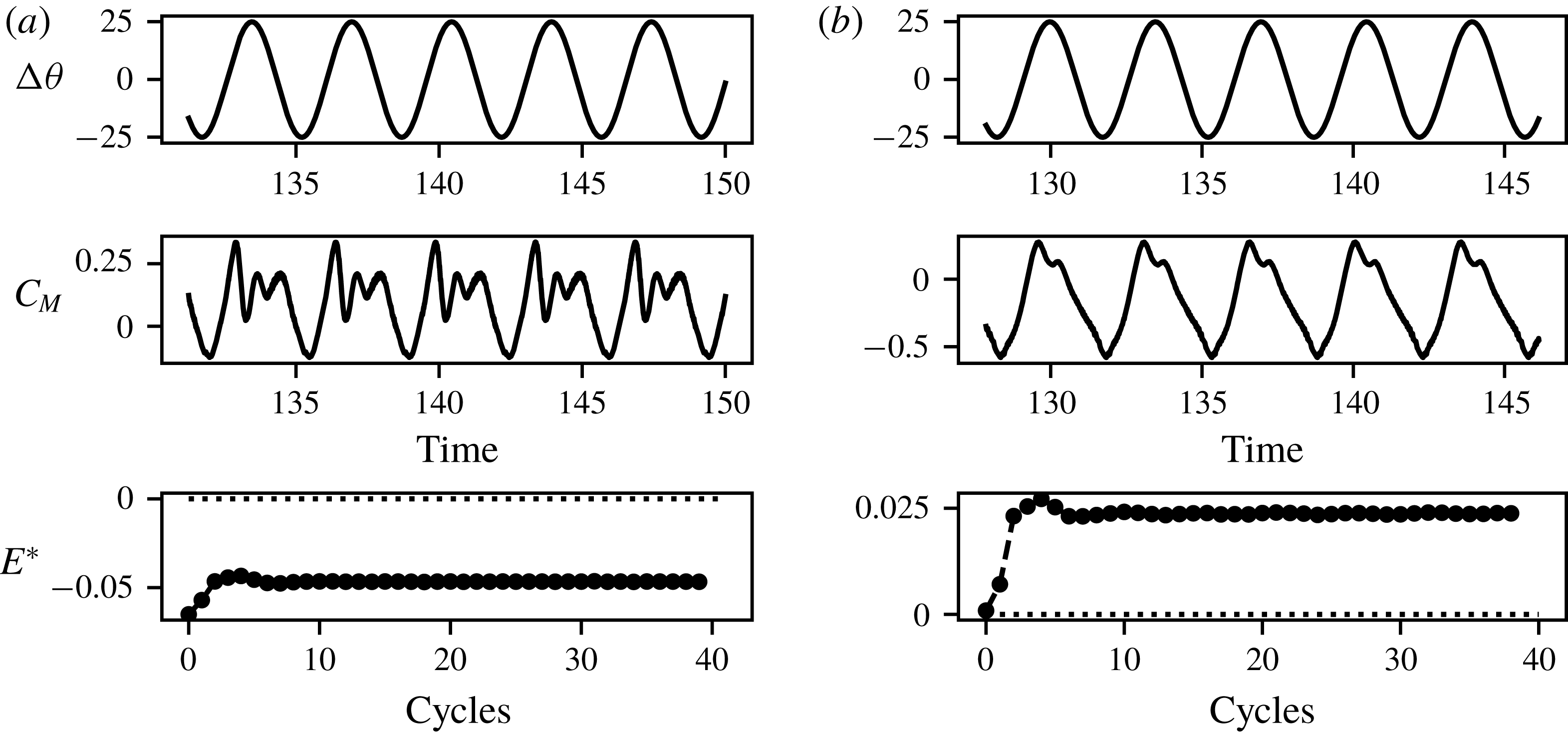
for the bifurcation to large amplitude oscillations. The phase difference between pitch and pitch moment is also a strong factor when considering the changes in the location of the elastic axis. This is demonstrated in figure 12 where we show time series plots of the pitch deflection and moment coefficient for an airfoil forced to oscillate at
 $A_{\unicode[STIX]{x1D703}}=25^{\circ }$
, about two different locations of the elastic axis. These sample cases show that changing the elastic axis, while retaining the kinematics, produces very different forcing on the airfoil. This is a result of the timing associated with the shedding as well as convection of vortices past the hinge location. These effects were also demonstrated in figure 1. The difference in timing leads to the case with
 $X_{e}^{\ast }=0.33$
being damped, while
 $X_{e}^{\ast }=0.50$
extracts energy. These examples suggest that the phase difference, and hence energy extraction, is indeed an important factor in analysing the response of flow-induced flutter.
Comparison of
 $\unicode[STIX]{x0394}\unicode[STIX]{x1D703}$
,
 $C_{M}$
and extracted energy
 $E_{f}^{\ast }$
, for airfoils forced to oscillate with
 $A_{\unicode[STIX]{x1D703}}=25^{\circ }$
and
 $f_{p}^{\ast }=0.25$
about two different hinge locations, (a)
 $X_{e}^{\ast }=0.33$
; (b)
 $X_{e}^{\ast }=0.50$
.

The aim in this section is to use our knowledge of the energy extraction, as described above, to understand the amplitude response of the dynamical system as a function of the various parameters explored in this study. To do this, we first create a map of energy transfer as a function of the parameters of interest. This is done by performing simulations of airfoils that are forced to undergo sinusoidal pitching oscillations over a range of amplitudes and frequencies, while holding the other parameters such as
 $X_{e}^{\ast }$
and
 $Re$
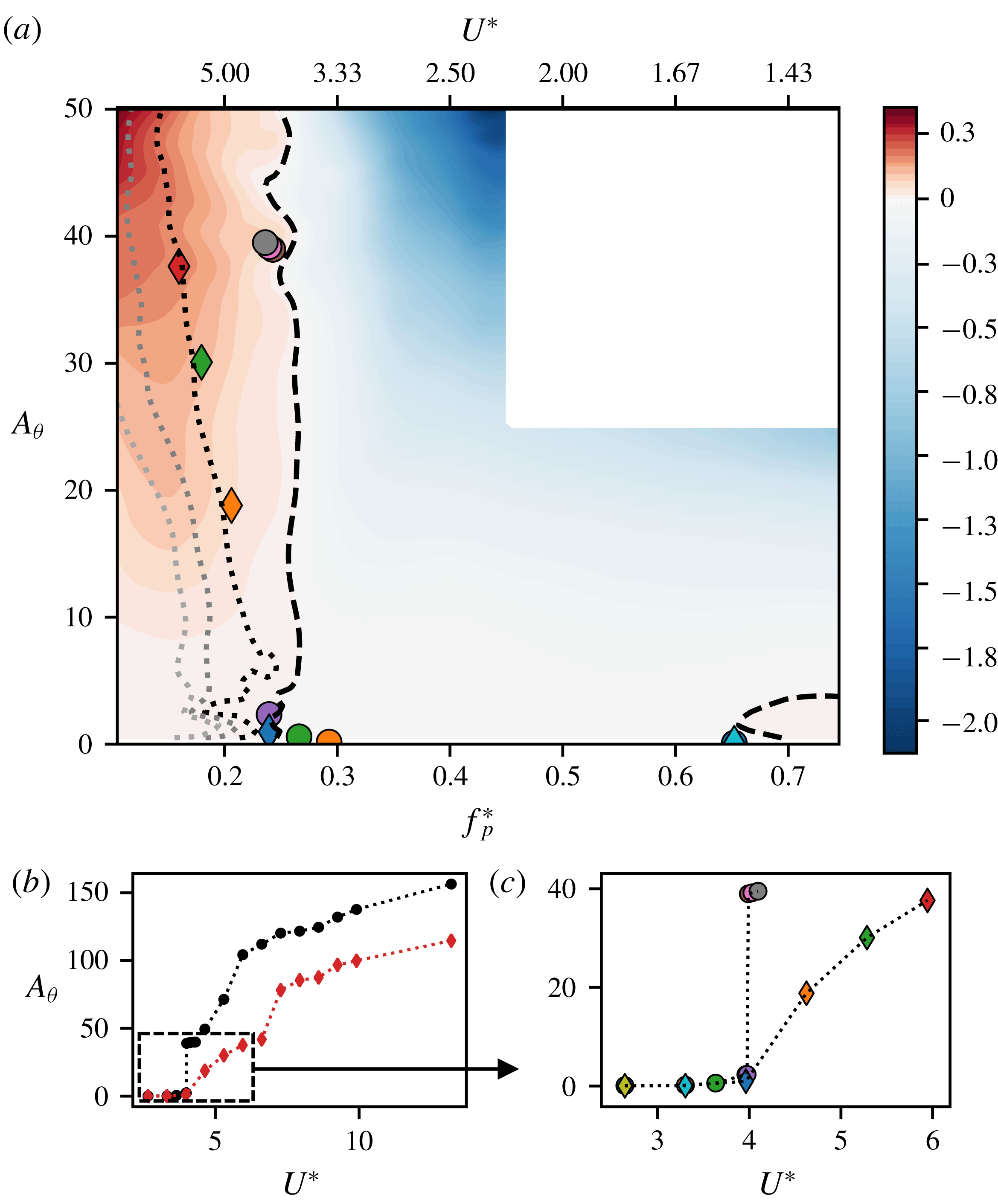
fixed. The pitching and pitch-moment data from each of these simulations is then used to calculate the energy extracted by the airfoil. The validity of these energy maps, which are obtained from forced oscillations, for the case of free, flow-induced oscillations rests primarily on the assumption that the free oscillations are strictly sinusoidal. We find that this condition is indeed satisfied to a very large degree for all the cases simulated here (see figures 2 and 5) and a sinusoidal fit to the pitching time series yields an R-square value of roughly 0.99 for nearly all cases studied. Indeed, energy maps have been used quite successfully to understand flow-induced vibration of bluff bodies (Morse & Williamson Reference Morse and Williamson2009) and Bhat & Govardhan (Reference Bhat and Govardhan2013) also demonstrated the use of an energy map to study flow-induced flutter of an airfoil.
(a) Contours of energy extraction,
 $E_{f}^{\ast }$
, as a function of oscillation amplitude and frequency for
 $X_{e}^{\ast }=0.50$
,
 $\unicode[STIX]{x1D703}_{0}=15^{\circ }$
. Symbols represent stationary state
 $f_{p}^{\ast }$
and
 $A_{\unicode[STIX]{x1D703}}$
for undamped (○) and damped (♢) flow-induced oscillation cases. Dashed and dotted lines represent undamped (
 $E_{f}^{\ast }=0$
) and damped (
 $E_{f}^{\ast }=E_{d}^{\ast }$
) equilibrium curves respectively.
 $E_{d}^{\ast }$
is calculated using
 $\unicode[STIX]{x1D701}=0.15$
for the darkest damped equilibrium curve, and increasing values of
 $\unicode[STIX]{x1D701}$
for subsequently lighter equilibrium curves (
 $\unicode[STIX]{x1D701}=0.30$
, 0.45); (b) reproduction of figure 10(a) with inset box showing range of
 $U^{\ast }$
and
 $A_{\unicode[STIX]{x1D703}}$
computed in the energy map; (c) zoom-in of flow-induced oscillation amplitudes for cases compared with the energy map.

The first map shown in figure 13 is for the case with
 $X_{e}^{\ast }=0.50$
and
 $Re=1000$
. This map is the result of a total of
 ${\sim}300$
simulations over a range of non-dimensional pitch frequencies
 $f_{p}^{\ast }=f_{p}C/U_{\infty }:[0.10,0.75]$
and pitch amplitudes
 $A_{\unicode[STIX]{x1D703}}:[0,50^{\circ }]$
. For each case, we simulate over 50 total cycles to ensure that a stationary state is achieved, and obtain
 $E_{f}^{\ast }$
by integrating over the last 20 cycles. The dashed line in the energy map corresponds to
 $E_{f}^{\ast }=0$
and the dotted line corresponds to
 $E_{f}^{\ast }=E_{d}^{\ast }$
, where
 $E_{d}^{\ast }$
is calculated using the value of structural damping previously specified in § 2.1. These represent potential equilibrium conditions in the case of flow-induced flutter.
The primary features in the map are the nearly vertical demarcation between regions of positive and negative energy transfer at approximately
 $f_{p}^{\ast }\approx 0.25$
and the small region of positive energy transfer around
 $f_{p}^{\ast }\approx 0.65$
. From this energy map, we expect that sustained flow-induced oscillations for cases with structural damping would occur in the region with
 $E_{f}^{\ast }>0$
, whereas cases without structural damping should saturate along the
 $E_{f}^{\ast }=0$
contour line. To verify this, we superimpose on this map, the stationary-state amplitude and frequencies from the flow-induced flutter simulations for
 $X_{e}^{\ast }=0.50$
. We find that for all these cases, the system saturates very close to the contour line corresponding to net energy equilibrium, i.e.
 $E_{f}^{\ast }=0$
for undamped oscillations and
 $E_{f}^{\ast }=E_{d}^{\ast }$
for damped oscillations. These observations provide clear confirmation of the validity of these energy maps as a tool for understanding the flow-induced flutter response.
Examining the energy maps further, we note that the nearly vertical
 $E_{f}^{\ast }=0$
contour line lies very close to the frequency corresponding to the reciprocal of the critical velocity, which is the frequency at which the bifurcation to large-amplitude oscillations occurs for the flow-induced oscillation with
 $X_{e}^{\ast }=0.50$
. This feature of the current energy map agrees qualitatively with that generated via experiments of Bhat & Govardhan (Reference Bhat and Govardhan2013), despite the fact that their Reynolds number is an order of magnitude larger than the current one and their pitch axis is at quarter chord. Also, the small region of positive energy transfer on the right side of the map has a frequency that corresponds to the Kármán oscillation mode identified earlier (see figure 4).
The topology of the energy map and the equilibrium curve provide useful insights regarding the dynamics of this configuration. For instance, the nearly vertical demarcation between the regions of energy growth and decay at
 $f_{p}^{\ast }\approx 0.25$
suggests that an undamped system would experience rapid growth in flutter amplitude with a relatively small decrease (increase) in pitch frequency (reduced velocity). Indeed, figure 10(a) shows that the undamped system exhibits what seems to be a subcritical bifurcation at
 $U^{\ast }\approx 4.0$
with a jump in amplitude of nearly
 $40^{\circ }$
. As the structural damping is increased, the equilibrium curve bends to the left (i.e. increasingly negative slope) indicating a smoother onset of flutter. Furthermore, increased damping significantly limits the maximum amplitude attained by the system. Other implications of the topology of the energy map for the system dynamics are explored in the next section.
4.2 Amplitude response for
 $X_{e}^{\ast }=0.33$

The case with
 $X_{e}^{\ast }=0.33$
exhibits a very complex, non-monotonic response with
 $U^{\ast }$
and we now demonstrate the utility of the energy maps in providing insight into this response. As shown in (4.1) and appendix A, oscillations in the absence of structural damping are expected to grow (decay) in regions of positive (negative)
 $E_{f}^{\ast }$
. The requirements for a stable equilibrium are
 $$\begin{eqnarray}E_{f}^{\ast }=0;\quad \text{d}E_{f}^{\ast }/\text{d}A<0.\end{eqnarray}$$
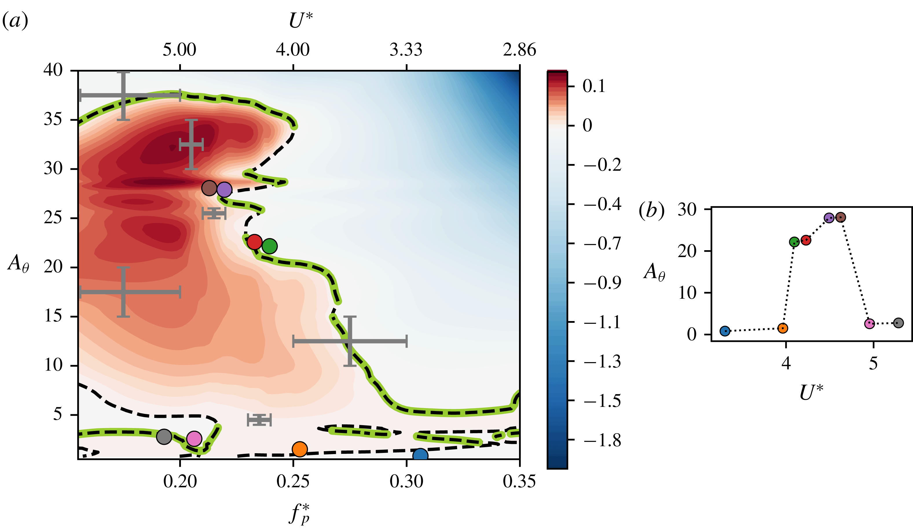
Figure 14 shows the energy map for this case which is generated as before by conducting
 ${\sim}200$
simulations of prescribed flutter over a large range of pitch frequencies and amplitudes. On this energy map, we have identified the curves corresponding to the equilibrium condition (
 $E_{f}^{\ast }=0$
) as well as the regions of stability on these equilibrium curves (
 $\text{d}E_{f}^{\ast }/\text{d}A<0$
). A number of qualitative observations can immediately be made regarding this energy map. First, the topology is very different from that for
 $X_{e}^{\ast }=0.50$
. Since free oscillations can only exist within the region of
 $E_{f}^{\ast }\geqslant 0$
, the energy map suggests an upper limit of
 $A_{\unicode[STIX]{x1D703}}\approx 40^{\circ }$
on the flow-induced oscillation amplitude in this case. The topology of the map is also extremely complicated: two main regions of energy growth and decay are separated by a complex equilibrium curve that extends over the entire range of frequencies considered here. There also exist multiple ‘islands’ with
 $E_{f}^{\ast }<0$
within the large region of energy growth in the low-amplitude (
 ${<}10^{\circ }$
) portion of the map, and this points to the possibility of multiple equilibrium states for a given conditions as well as abrupt changes in oscillation amplitude with changes in the underlying parameters.
(a) Energy map for
 $X_{e}^{\ast }=0.33$
and
 $\unicode[STIX]{x1D703}_{0}=15^{\circ }$
, with the equilibrium curve (
 $E_{f}^{\ast }=0$
) shown as a dashed line, and stable equilibrium (
 $E_{f}^{\ast }=0$
,
 $\text{d}E^{\ast }/\text{d}A<0$
) highlighted along the equilibrium curve (thick line); (b) maximum pitch deflections versus
 $U^{\ast }$
for cases with
 $\unicode[STIX]{x1D701}=0$
corresponding to figure 10(b); the stationary-state oscillation amplitude and frequency of all cases shown in (b) are plotted on the energy map using circles (○). Also shown on the energy map are bars indicating the local resolution in
 $f_{p}^{\ast }$
and
 $A_{\unicode[STIX]{x1D703}}$
in various regions of the energy map. Local regions of the map that contain complex topological features have been provided with higher resolution.

To compare our prediction for the equilibrium positions on this energy map, we superimpose the stationary-state locations of our flow-induced data for
 $X_{e}^{\ast }=0.33$
on the energy map using circle (○) symbols. This data set was described earlier in § 3.5 (see figure 10
b) and is also shown as maximum pitch deflection versus
 $U^{\ast }$
in figure 14(b). These cases correspond to zero structural damping, and are hence expected to lie along stable equilibria identified on the
 $E_{f}^{\ast }=0$
curve. In figure 14 we see that there is again very good agreement between the flow-induced oscillations data and the energy map. The slight discrepancies in this comparison are a result of the finite resolution of the energy map, which is not able to fully resolve the complicated structure of the map. This is especially apparent at very small oscillation amplitudes, where multiple equilibria exist in close proximity to each other. Hence on figure 14 we have also plotted error bars at various locations indicating the local step size in
 $f_{p}^{\ast }$
and
 $A_{\unicode[STIX]{x1D703}}$
used in computing generating the energy map.
In spite of the difficulty in fully resolving the topology of the energy map, it allows us to explain the complex, non-monotonic response of the flow-induced flutter for the undamped
 $X_{e}^{\ast }=0.33$
case. The map clearly shows that for
 $f_{p}^{\ast }>0.25$
 $(U^{\ast }<4)$
the system is trapped in a lower branch of the energy map which has very small amplitude. However, as
 $f_{p}^{\ast }$
reduces below
 $0.25$
 $(U^{\ast }>4)$
the lower branch all but disappears. Thus for the case with
 $f_{p}^{\ast }>0.237\;(U^{\ast }=4.22)$
the system finds itself in a region of positive energy growth and the amplitude grows and saturates at the first stable equilibrium along the vertical line representing its natural frequency in the map, which is approximately
 $A_{\unicode[STIX]{x1D703}}=22^{\circ }$
. Between
 $f_{p}^{\ast }=0.22$
and 0.25, the system continues to grow to the large amplitudes associated with the upper equilibrium curve, however, for
 $f_{p}^{\ast }<0.22\;(U^{\ast }>4.5)$
, a lower, stable equilibrium branch appears and the system locks on this lower branch. Hence, after the bifurcation to large-amplitude oscillations at approximately
 $U^{\ast }=4$
, the amplitude of the system drops significantly (
 ${\approx}3^{\circ }$
for
 $U^{\ast }>4.54$
. In contrast, for the case of
 $X_{e}^{\ast }=0.50$
, there is no such lower branch in the energy map (see figure 13). Hence the oscillation amplitude increases monotonically along the
 $E_{f}^{\ast }=0$
curve for that case.
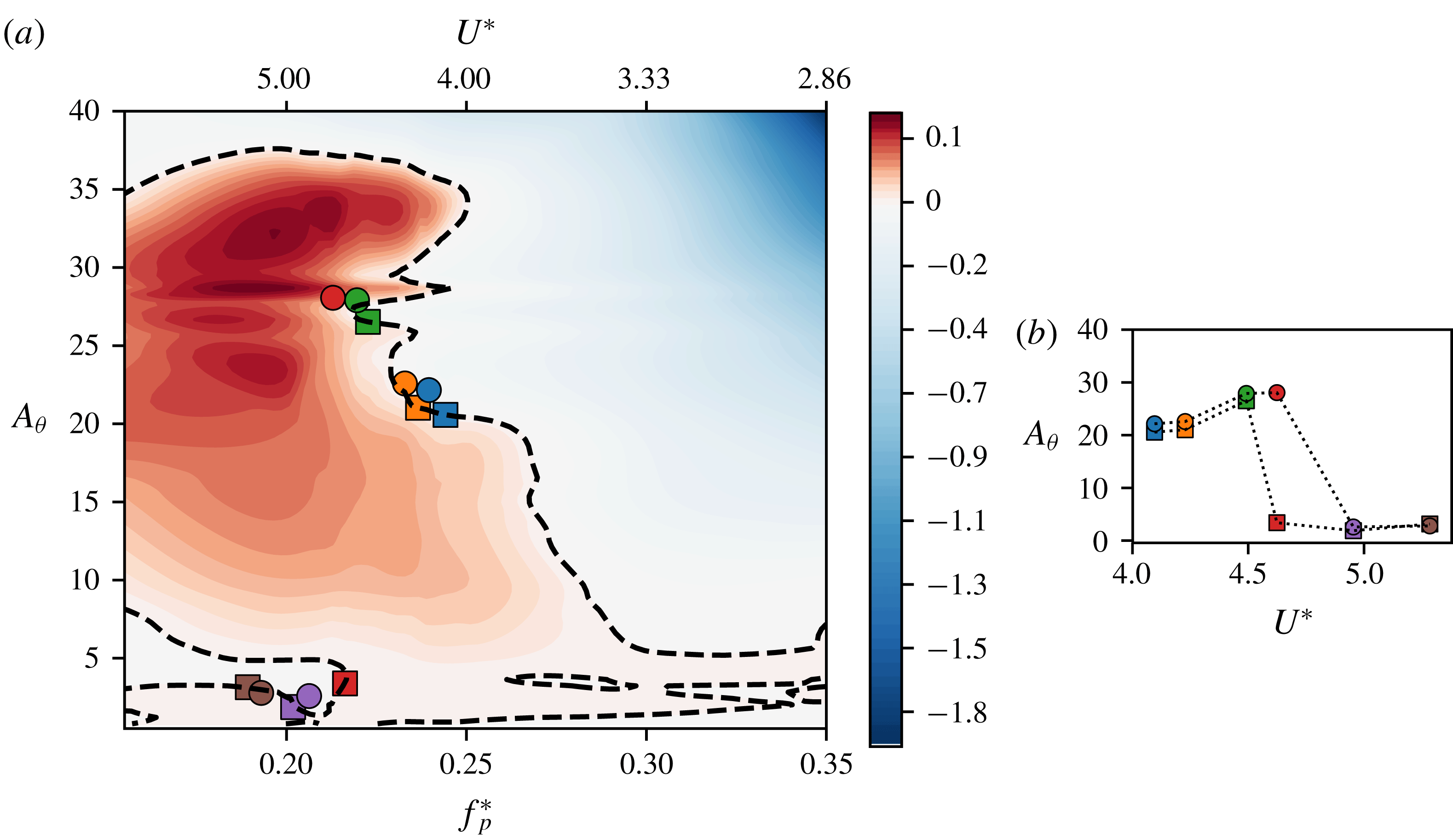
Prediction of
 $A_{\unicode[STIX]{x1D703}}$
using (A 5), compared with calculations from flow-induced oscillation simulations. Here,
 $X_{e}^{\ast }=0.33$
and
 $\unicode[STIX]{x1D703}_{0}=15^{\circ }$
; (a) stationary-state amplitudes and frequencies from the model (▫), and flow-induced simulations corresponding to figure 14 (○) plotted on the energy map; (b) corresponding amplitudes plotted against
 $U^{\ast }$
using the same symbols as in (a).

Having established that the energy map indeed describes the stationary states of the flow-induced flutter system, we now demonstrate its use in making a priori predictions of the stationary-state amplitude without the need for flow simulations. This serves as a demonstration of the energy map as a predictive tool as well as a validation of our model for amplitude growth (shown in appendix A). From (A 5), we can calculate the amplitude growth of an oscillator at every cycle, with the knowledge of its spring stiffness and cycle-wise energy extraction. As mentioned before, this assumes that the oscillations are purely sinusoidal and occur at the natural frequency of the system. With these assumptions, we can pick the oscillation frequency of the system and predict the growth of amplitude based on the energy map and an initial condition. We iterate (A 5) using a semi-implicit Crank–Nicholson scheme, and the iteration is performed until a stationary state is achieved. We demonstrate this for some selected cases in figure 15, where we compare the amplitude response observed in flow-induced oscillations (○), with that predicted by our model (▫). We see that we are able to predict the amplitude response accurately for most cases by purely using the energy map. One case however, with
 $U^{\ast }=4.62$
, does not agree with the model’s predictions. As is apparent in figure 15(a), this is because the energy map computed here predicts the existence of a small-amplitude stable equilibrium at this oscillation frequency. This is a result of finite resolution in computing the map, as was mentioned earlier. Furthermore, the fact that this region of the map is especially sensitive to small changes in frequency and amplitude magnifies the finite resolution effects. This sensitivity of the energy prediction to input conditions was also observed by Leontini et al. (Reference Leontini, Stewart, Thompson and Hourigan2006).
4.3 Transient response
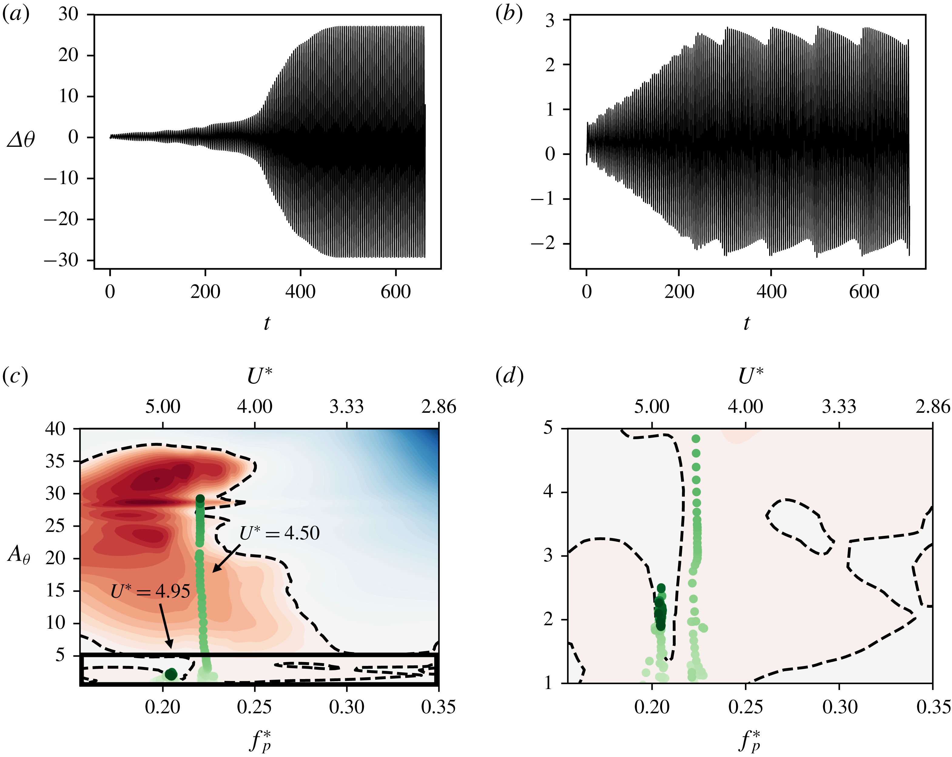
The energy maps also allow us to understand the transient response of the various flow-induced flutter cases. In figure 16 we plot the pitching amplitude time series and trajectories of two cases of flow-induced flutter, where the circles represent the location of the oscillator on the frequency–amplitude space during each cycle. This is calculated by dividing the pitch response time series into individual cycles, and calculating the amplitude and time scale associated with each cycle. In the case of
 $U^{\ast }=4.50$
, we observe that the trajectory of the system follows a nearly vertical line on the energy map. This is because this case corresponds to the post-bifurcation regime, and the frequency is selected based on the natural frequency of the system. The system starts at rest, close to
 $\unicode[STIX]{x0394}\unicode[STIX]{x1D703}=0$
, and the amplitude grows due to the positive energy extracted from the flow. We see in figure 16(c) that this amplitude growth occurs until it reaches a stable equilibrium position corresponding to its oscillation frequency. However, before reaching this stationary state, the oscillator spends a long time close to a small-amplitude equilibrium region, as shown by the density of circles in the zoomed-in trajectory shown in figure 16(d). The effect of this is also seen in the pitch amplitude time series of this case, shown in figure 16(a). The system exhibits small amplitude oscillations for an extended period of time, before a sudden growth in amplitude caused by its escape from the small-amplitude stable region.
Comparison of two flow-induced oscillation cases with
 $U^{\ast }=4.50$
and
 $U^{\ast }=4.95$
. Top panels show time series of pitch oscillations for (a)
 $U^{\ast }=4.50$
and (b)
 $U^{\ast }=4.95$
; (c) amplitude–frequency trajectories of these cases on the energy map. Each circle represents the amplitude and frequency during one oscillation cycle. The colour intensity represents time; (d) zoom-in of trajectories in the inset box shown in (c).

On slightly increasing
 $U^{\ast }$
to 4.95, the system gets trapped in the low-amplitude stable branch, as seen in figure 16(c). Further, we see from the pitch response time series in figure 16(b) that the oscillation amplitude in this case shows an interesting beating behaviour. This suggests that the oscillator is trapped in a bi-stable region that allows it to move between two stable equilibrium positions. While the exact structure of this stable region is difficult to resolve, figure 16(d) shows that the system gets trapped in a nearly vertical branch of
 $E_{f}^{\ast }=0$
that would allow the existence of multiple stable regions. Further, the vertical spread of instantaneous amplitudes after the system has reached a stationary state (shown by the spread of circles) suggests that the system does indeed move between two equilibrium states. The analysis of these cases shows the utility of the energy map in analysing the stationary-state response, as well as the trajectory of the oscillator from the initial condition to the stationary state. We also see that the complicated structure of the energy map leads to interesting behaviour in the pitching response of this system, which would be very difficult to interpret without knowledge of the corresponding energy map.
(a) Energy map for
 $X_{e}^{\ast }=0.33$
, with equilibrium curve, stable equilibria and stationary-state frequency and amplitudes as in figure 14. Also shown are cases demonstrating hysteresis, represented by diamonds (♢), by continuing along the directions indicated by the arrows; (b) the stationary-state oscillation amplitude of all cases shown in the energy map, plotted against
 $U^{\ast }$
using the same symbols.

Trajectories of flow-induced oscillation cases showing hysteresis. Top panels show time series of pitch oscillations for (a)
 $U^{\ast }=3.30$
and (b)
 $U^{\ast }=4.95$
, where the lighter time series represents the approach to the initial state (before hysteresis) and the darker time series shows the evolution after the change of
 $U^{\ast }$
; (c) amplitude–frequency trajectories of the case with
 $U^{\ast }=3.30$
on the energy map, where the approach to the initial condition as well as the subsequent evolution at
 $U^{\ast }=3.30$
is shown; (d) amplitude–frequency trajectories of the case with
 $U^{\ast }=4.95$
.

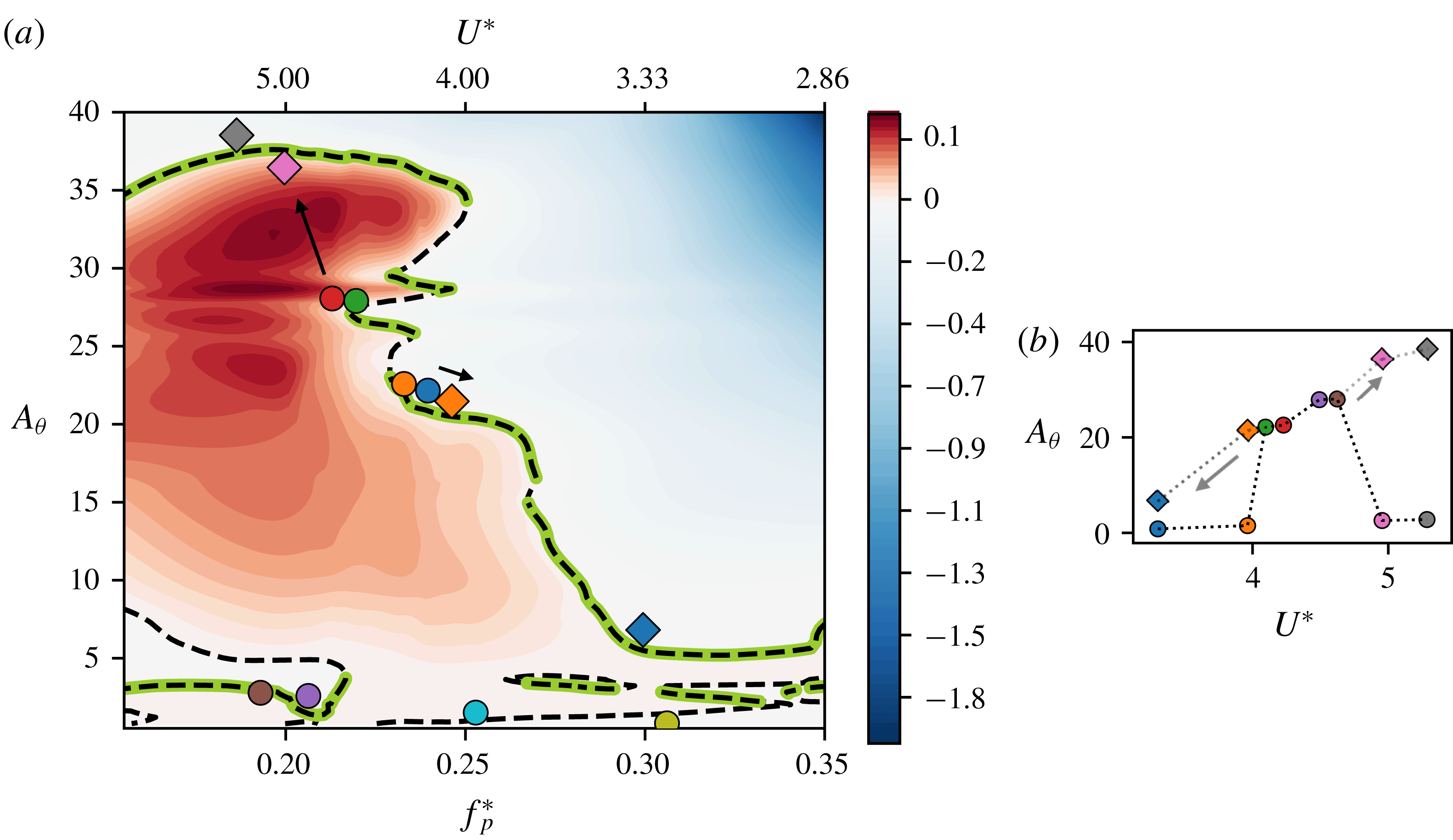
The energy map also allows us to predict hysteretic behaviour due to the presence of multiple stable equilibria at particular oscillation frequencies. In figure 17 we show the energy map, as in figure 14, with additional cases that demonstrate hysteresis shown using diamond (♢) symbols. These simulations were carried out using a previously computed stationary state along the equilibrium curve as an initial condition, changing the value of
 $U^{\ast }$
, and allowing the dynamics to evolve to a new stationary state. We use arrows pointing from the initial to the final stationary state to denote the change in
 $U^{\ast }$
in figure 17. We see that these cases agree with the equilibrium and stability conditions predicted by the energy map too.
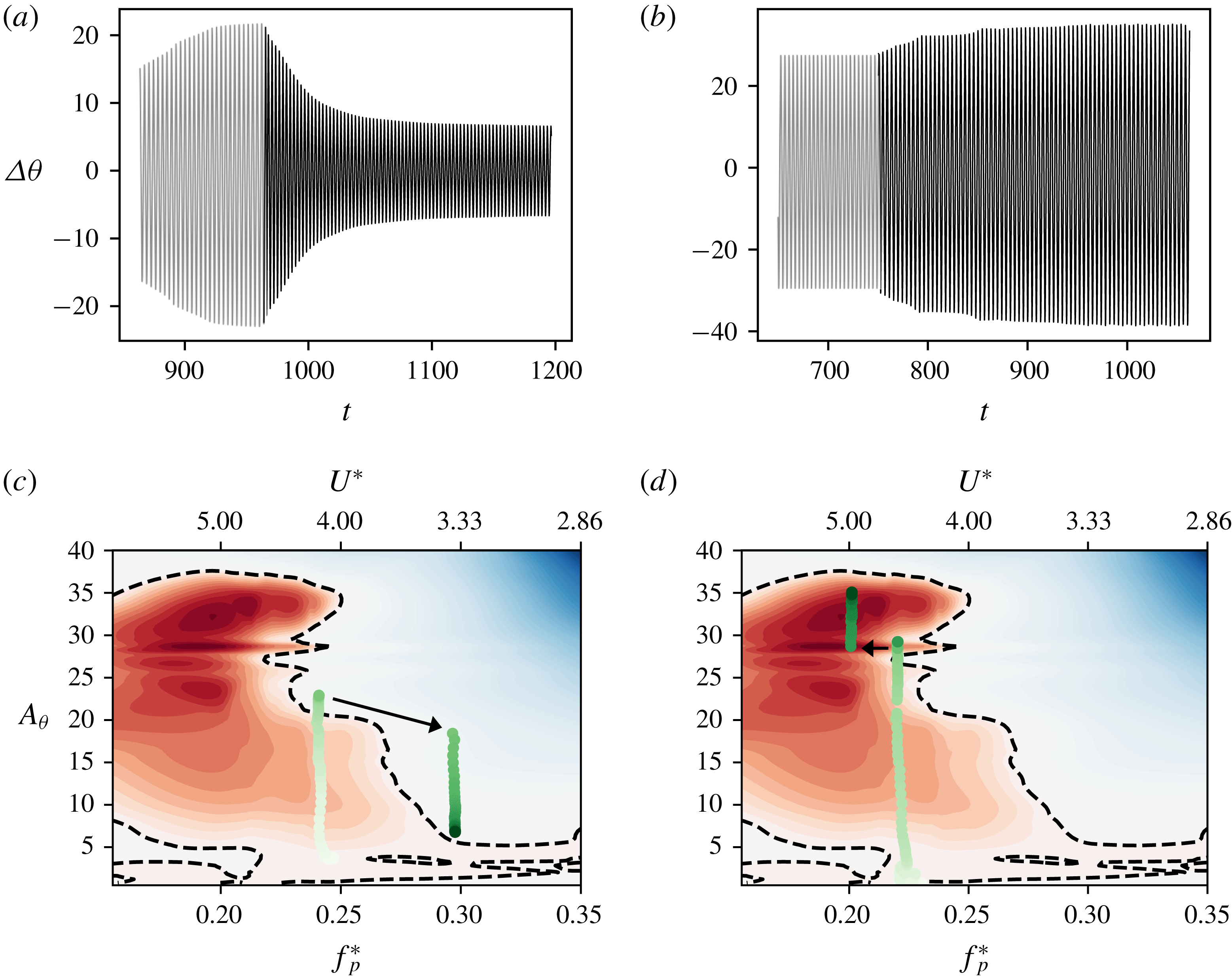
The transient response of these cases is especially interesting to analyse as it also demonstrates the ability to use these energy maps in flutter amplitude control. In figure 18 we plot the pitching time series and trajectories of two such cases showing hysteretic behaviour with
 $U^{\ast }=3.30$
and
 $U^{\ast }=4.95$
. Figures 18(a) and 18(b) show time series plots of pitching amplitude, where the grey portion represents the last few cycles of the case used as an initial condition, and the black time series shows the subsequent amplitude response leading to the new stationary state. In figures 18(c) and 18(d) we show the trajectories of these cases where the circles show the state of the system on the frequency–amplitude space during each oscillation cycle. Here we show the trajectory leading up to the stationary state that is used as an initial condition, as well as the trajectory from the previous stationary state to the new one. The change in
 $U^{\ast }$
is indicated by the arrow.
For
 $U^{\ast }=3.30$
, the case using the static initial condition shows very small-amplitude oscillations (
 $A_{\unicode[STIX]{x1D703}}<1^{\circ }$
) as seen in figure 10(b) and is described by the pre-bifurcation regime on § 3.3. However, when initialized with an oscillation amplitude
 ${\sim}25^{\circ }$
, we see that it reaches a stationary-state amplitude of approximately
 $10^{\circ }$
. This new stationary state is achieved through a loss of energy, which is different from all the cases analysed in this paper so far. The loss of energy is a consequence of the fact that the initial amplitude of oscillation, which corresponds to a stable equilibrium at a different natural frequency, is in a region of negative energy transfer at the natural frequency corresponding to
 $U^{\ast }=3.30$
. This results in a reduction in amplitude of oscillation as described by (A 6), until it reaches a new stable equilibrium. This is an example of the ability to reduce the amplitude of flutter using a knowledge of the energy map.
The case of
 $U^{\ast }=4.95$
shows a case that is initialized using a stationary state on one portion of the equilibrium curve, and ends up on higher-amplitude portion of the curve on changing its natural frequency. This occurs as the change in natural frequency pushes the system into a region of positive energy transfer, as indicated by the arrow in figure 18(d). Due to continuous extraction of energy from the flow, the amplitude grows until it reaches a new stable equilibrium. It must be noted that this is the same
 $U^{\ast }$
value shown in figures 16(b) and 16(d), where the static initial condition was used.
With these above examples we have been able to demonstrate the use of the idea of an energy map to analyse the dynamics of the flow-induced oscillator a priori, based on our knowledge of the frequency selection mechanism. We have also been able to explain the bizarre non-monotonic amplitude response seen in the case of
 $X_{e}^{\ast }=0.33$
using this tool.
5 Conclusions
We have carried out a study of flow-induced airfoil flutter at a chord-based Reynolds number of 1000 using high-fidelity modelling of the fluid dynamics coupled with a linear structural model for deflection in pitch. The objectives of this work were twofold – to carry out a systematic study of the parameters affecting the dynamics of wing flutter, and to demonstrate the use of the energy exchange between the fluid and the structure as a way to analyse the flutter behaviour and its dependence on various parameters such as spring stiffness, elastic-axis location and mean angle of attack.
It is shown that for cases that exhibit significant flutter, the onset of flutter occurs at a reduced velocity (
 $U^{\ast }=U_{\infty }/Cf_{s}$
) which is dependent on the initial angle of attack. Simulations are used to determine a time scale (
 $T_{v}$
) corresponding to the relaxation of a pitch perturbation, which provides a more appropriate flow time scale for this problem. A reduced velocity defined based on this time scale, i.e.
 $U_{v}^{\ast }=f_{s}^{-1}/T_{v}$
leads to the simple condition that flutter will occur for
 $U_{v}^{\ast }>1$
, irrespective of the angle of attack. This condition provides a phenomenological basis for the onset of flutter: the natural time scale of the system (
 $f_{s}^{-1}$
) should be larger than the time scale (
 $T_{v}$
) of the flow so as to enable constructive coupling between the flow and the structure and amplification of a pitch perturbation. Finally, we provide some evidence that the time scale
 $T_{v}$
is proportional to the thickness of the boundary layer at the point of separation over the suction surface of the static airfoil, thereby connecting this time scale to the intrinsic instability of the separated shear layer.
In the second part of this study, we demonstrated the use of ‘energy maps’, as an analytical tool to analyse the complex flow-induced flutter response of the airfoil. Energy maps are generated by computing the rate of energy exchange between the airfoil and the flow for airfoils undergoing prescribed pitch flutter over a range of amplitude and frequencies. The topology of the energy maps changes significantly with the location of the elastic axis and we show that the energy maps provide a very effective means for interpreting complex behaviour such as non-monotonic saturation amplitudes, hysteresis, subcritical and supercritical bifurcations and complex limit-cycle behaviour. Furthermore, we show that a simple mathematical model based on the energy maps can even predict the saturation amplitude without the need for flow-induced flutter simulation.
The current study and analysis has a number of limitations. The simulations are two-dimensional, limited to low Reynolds numbers and they do not inform about how flutter would be affected by the introduction of new time scales and strong intrisic three-dimensional effects associated with higher Reynolds numbers. The current study also does not address structures with multiple intrinsic modes/frequencies of flutter. We believe that the current approach of generating energy maps would be equally valuable in such systems, however the dynamics would live in a higher-dimensional energy map than demonstrated here. In general, each additional mode would correspond to an added dimension on the energy map. However, for the specific case of plunge oscillations with small amplitude or frequency, the added dimension could possibly be modelled in a quasi-steady manner as an effective angle of attack or using the model of Theodorsen (Reference Theodorsen1935). It is also worth noting that in coupled pitch–plunge systems, we expect the mechanism for the onset of the instability in each mode to be similar to that described in § 3.4, i.e. a competition between the natural time scale of the structure and the relaxation time scale of the forcing. However, it is possible that the growth of plunge instability could force the growth of pitch oscillations, and vice versa, due to the presence of subcritical response branches, as seen in this study. Another limitation to note is that the energy maps can have highly complex topologies that may be difficult to resolve fully. This also raises the question as to what features of the flow determine the topology of the energy map? This question is related primarily to the vortex dynamics in this coupled system, and such questions are interesting directions for future research.
Acknowledgement
This work is supported by the Air Force Office of Scientific Research grant no. FA 9550-16-1-0404, monitored by Dr G. Abate. The development of the flow solver used here has benefited from NSF grant CBET-1511200.
Appendix A. Model for amplitude growth
In this section, we present a mathematical model for amplitude growth and equilibrium for the flow-induced flutter of the airfoil. Multiplication of
 $\dot{\unicode[STIX]{x1D703}}$
to (2.2) as follows:
 $$\begin{eqnarray}I^{\ast }\ddot{\unicode[STIX]{x1D703}}\dot{\unicode[STIX]{x1D703}}+k^{\ast }(\unicode[STIX]{x1D703}-\unicode[STIX]{x1D703}_{0})\dot{\unicode[STIX]{x1D703}}=C_{M}\dot{\unicode[STIX]{x1D703}}-b^{\ast }\dot{\unicode[STIX]{x1D703}}\dot{\unicode[STIX]{x1D703}}\end{eqnarray}$$
results in a simple energy balance describing the growth of energy in the oscillator
 $$\begin{eqnarray}\;\Longrightarrow \;\frac{\text{d}}{\text{d}t}\left(\frac{1}{2}I^{\ast }\dot{\unicode[STIX]{x1D703}}^{2}\right)+\frac{\text{d}}{\text{d}t}\left(\frac{1}{2}k^{\ast }\unicode[STIX]{x1D703}^{2}\right)=\frac{\text{d}e_{f}^{\ast }}{\text{d}t}-\frac{\text{d}e_{d}^{\ast }}{\text{d}t}=\frac{\text{d}e^{\ast }}{\text{d}t},\end{eqnarray}$$
where
 $e_{f}^{\ast }$
is the energy extracted by the airfoil from the flow and
 $e_{b}^{\ast }$
is the energy lost to structural damping. Integrating this equation over an oscillation cycle with time period
 $T$
, where the beginning of the cycle is at time
 $t_{n}$
, results in an equation for the change of amplitude over the oscillation cycle
 $$\begin{eqnarray}I^{\ast }[\dot{\unicode[STIX]{x1D703}}^{2}(t_{n}+T)-\dot{\unicode[STIX]{x1D703}}^{2}(t_{n})]+k^{\ast }[\unicode[STIX]{x1D703}^{2}(t_{n}+T)-\unicode[STIX]{x1D703}^{2}(t_{n})]=2[e^{\ast }(t_{n}+T)-e^{\ast }(t_{n})]=2E^{\ast },\end{eqnarray}$$
where
 $E^{\ast }$
is the net energy gain of the structure over one cycle. Assuming a purely sinusoidal form for
 $\unicode[STIX]{x1D703}$
and
 $\dot{\unicode[STIX]{x1D703}}$
, i.e.
 $\unicode[STIX]{x1D703}=A_{\unicode[STIX]{x1D703}}\sin \unicode[STIX]{x1D714}t$
where
 $\unicode[STIX]{x1D714}^{\ast }=2\unicode[STIX]{x03C0}/T$
, results in the following equation for the change in amplitude over an oscillation cycle
 $$\begin{eqnarray}A_{\unicode[STIX]{x1D703}}^{2}(t_{n}+T)-A_{\unicode[STIX]{x1D703}}^{2}(t_{n})=\frac{2E^{\ast }}{I^{\ast }\unicode[STIX]{x1D714}^{2}\cos ^{2}\unicode[STIX]{x1D714}t+k^{\ast }\sin ^{2}\unicode[STIX]{x1D714}t}.\end{eqnarray}$$
Assuming the oscillation occurs at the natural structural frequency, i.e.
 $\unicode[STIX]{x1D714}=\sqrt{k^{\ast }/I^{\ast }}$
, we obtain the following equation for amplitude growth in the regime of oscillation at the natural frequency:
 $$\begin{eqnarray}\displaystyle & \displaystyle A_{\unicode[STIX]{x1D703}}^{2}(t_{n}+T)-A_{\unicode[STIX]{x1D703}}^{2}(t_{n})=\frac{2E^{\ast }}{k^{\ast }}, & \displaystyle\end{eqnarray}$$
 $$\begin{eqnarray}\displaystyle & \displaystyle \;\Longrightarrow \;A_{\unicode[STIX]{x1D703}}(t_{n}+T)-A_{\unicode[STIX]{x1D703}}(t_{n})=\frac{E^{\ast }}{k^{\ast }\bar{A}_{\unicode[STIX]{x1D703}}}, & \displaystyle\end{eqnarray}$$
where
 $\bar{A}_{\unicode[STIX]{x1D703}}=[A_{\unicode[STIX]{x1D703}}(t_{n}+T)+A_{\unicode[STIX]{x1D703}}(t_{n})]/2$
.
This is the Poincaré map of this dynamical system. Equilibrium is attained when
 $A_{\unicode[STIX]{x1D703}}(t_{n}+T)=A_{\unicode[STIX]{x1D703}}(t_{n})$
, and this corresponds to
 $$\begin{eqnarray}E^{\ast }=0.\end{eqnarray}$$
The equilibrium may be stable or unstable, and (A 6) also allows us to derive a linearized stability condition for this system. For a system of the form
 $A_{n+1}={\mathcal{F}}(A_{n})$
, where
 $n$
is the index of the return map, and
 ${\mathcal{F}}$
is some functional form, linear stability requires
 $\text{d}{\mathcal{F}}/\text{d}A<1$
(Strogatz Reference Strogatz2018). For our system, this gives the following condition for stability
 $$\begin{eqnarray}\frac{\text{d}}{\text{d}A_{\unicode[STIX]{x1D703}}}\left(A_{\unicode[STIX]{x1D703}}+\frac{E^{\ast }}{k^{\ast }\bar{A}_{\unicode[STIX]{x1D703}}}\right)<1\;\Longrightarrow \;\frac{\text{d}E^{\ast }}{\text{d}A_{\unicode[STIX]{x1D703}}}<0.\end{eqnarray}$$
Thus, the above indicates that a system allowed to flutter freely will equilibrate only when conditions (A 7) and (A 8) are satisfied simultaneously. Thus, a map of
 $E^{\ast }$
as a function of pitch frequency and amplitude could be used to understand, and even predict the response of the system. We note that this concept has previously been employed by other groups, primarily in the context of bluff body vibrations (Morse & Williamson Reference Morse and Williamson2009; Kumar et al.
Reference Kumar and Mittal2016). Furthermore, the equilibrium conditions arrived at here are the same as those employed in these previous studies.
Appendix B. Grid convergence and code validation
Time series of (a) moment, and (b) lift coefficients, for the three grids tested.

A grid convergence study was performed using forced oscillations of the truncated NACA0015 airfoil used in this study. The oscillations were performed about
 $\unicode[STIX]{x1D703}_{0}=20^{\circ }$
, with amplitude
 $A_{\unicode[STIX]{x1D703}}=20^{\circ }$
and frequency
 $f_{p}^{\ast }=0.15$
. The baseline grid tested consisted of
 $384\times 320$
grid cells. This corresponds to a resolution of approx. 125 cells along the chord of the airfoil. This grid was compared to those with
 $480\times 448$
and
 $544\times 544$
grid cells, which correspond to 192 and 237 cells along the chord, respectively. These refined grids are
 $2.3\times$
, and
 $3.6\times$
the size of the baseline grid, in terms of total grid cells. In figure 19 we show comparisons of the time series of lift coefficient and moment coefficient for these three grids. The mean and root mean square (r.m.s.) lift coefficient differ by 3.92 % and 1.2 % respectively between the baseline and
 $2.3\times$
grid, and 0.96 % and 1.51 % respectively between the baseline and
 $3.6\times$
grid. The corresponding difference in mean and r.m.s. moment coefficient is 1.78 % and 1.07 % between the baseline and
 $2.3\times$
grid, and 0.84 % and 2.05 % between the baseline and
 $3.6\times$
grid.
Time series of (a) pitch angle; (b) moment coefficient; and (c) lift coefficients, for flow-induced oscillations at
 $U^{\ast }=6.8$
using the Baseline and
 $2.3\times$
grids.

The grid convergence demonstrated above, while performed for forced oscillations, is expected to be a reasonably good demonstration of grid convergence for the flow-induced system as well. This is due to the fact that the only term in the dynamical equation for the solid (2.2) that depends on the grid is
 $C_{M}$
, which we have shown, is well converged. Further, in order to obtain statistics at a stationary state for the flow-induced system, Courant–Friedrichs–Lewy (CFL) criterion-related constraints would require simulations with as many as 2 000 000 time steps on the finer grids. This makes such an exercise computationally cost prohibitive. However, in order to strengthen this demonstration of our grid convergence, we have performed a comparison of the baseline and
 $2.3\times$
grid for a flow-induced oscillation simulation during the transient, amplitude growth phase at
 $U^{\ast }=6.8$
and
 $\unicode[STIX]{x1D703}_{0}=15^{\circ }$
. Plots for the pitch angle, and coefficients of moment and lift versus time are shown in figure 20. We see that the mean and r.m.s. lift coefficient differ by 0.57 % and 1.56 % respectively. The mean and r.m.s. moment coefficients differ by 3.78 % and 1.22 % respectively. The maximum pitching amplitude differs by 6.44 %.
Flow-induced oscillation amplitude of a circular cylinder versus mass-damping parameter
 $\unicode[STIX]{x1D6FD}=8\unicode[STIX]{x03C0}^{2}St^{2}m\unicode[STIX]{x1D701}/\unicode[STIX]{x1D70C}D^{2}$
. Results from the present code are shown using symbols and are compared with results from Blackburn & Karniadakis (Reference Blackburn and Karniadakis1993) shown as a dashed line.

Further, we have made various comparisons of results from the code used in this work with previous studies, in addition to the validation already mentioned in Mittal et al. (Reference Mittal, Dong, Bozkurttas, Najjar, Vargas and von Loebbecke2008). Specifically, force coefficients as well as Strouhal numbers predicted by ViCar3D for flow over static airfoils match very well with existing literature. These results are not shown here for the sake of brevity. In order to validate our fluid–structure interaction solver, we have performed simulations of flow-induced vibration of circular cylinders and compared our amplitude response with the results of Blackburn & Karniadakis (Reference Blackburn and Karniadakis1993). In figure 21 we show the amplitude response of a freely vibrating cylinder at
 $Re_{D}=200$
with
 $m^{\ast }=m/\unicode[STIX]{x1D70C}D^{2}=10$
, against the mass-damping parameter
 $\unicode[STIX]{x1D6FD}=8\unicode[STIX]{x03C0}^{2}St^{2}m\unicode[STIX]{x1D701}/\unicode[STIX]{x1D70C}D^{2}$
. Here,
 $St,m,\unicode[STIX]{x1D701},\unicode[STIX]{x1D70C}$
, and
 $D$
are the vortex shedding Strouhal number, mass, damping ratio, fluid density and cylinder diameter respectively. The symbols show results from our simulations and the dashed line is from the work of Blackburn & Karniadakis (Reference Blackburn and Karniadakis1993). The agreement is quite reasonable.