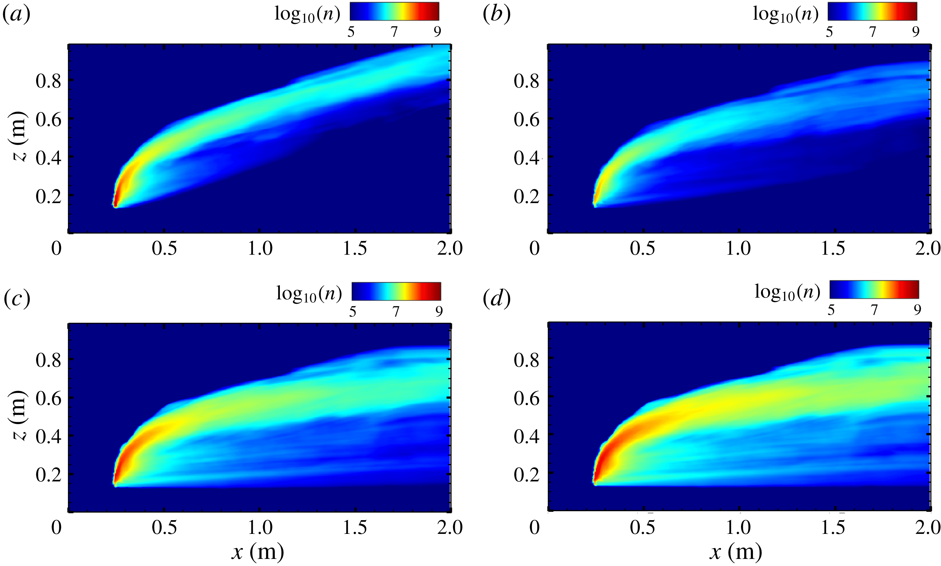
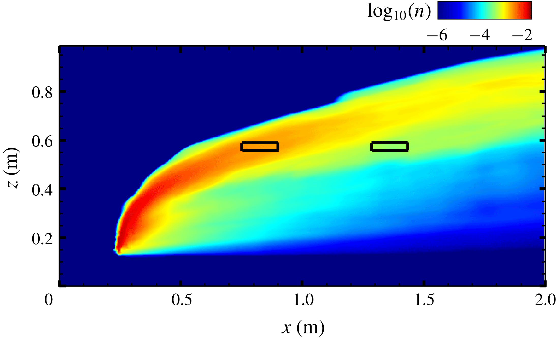
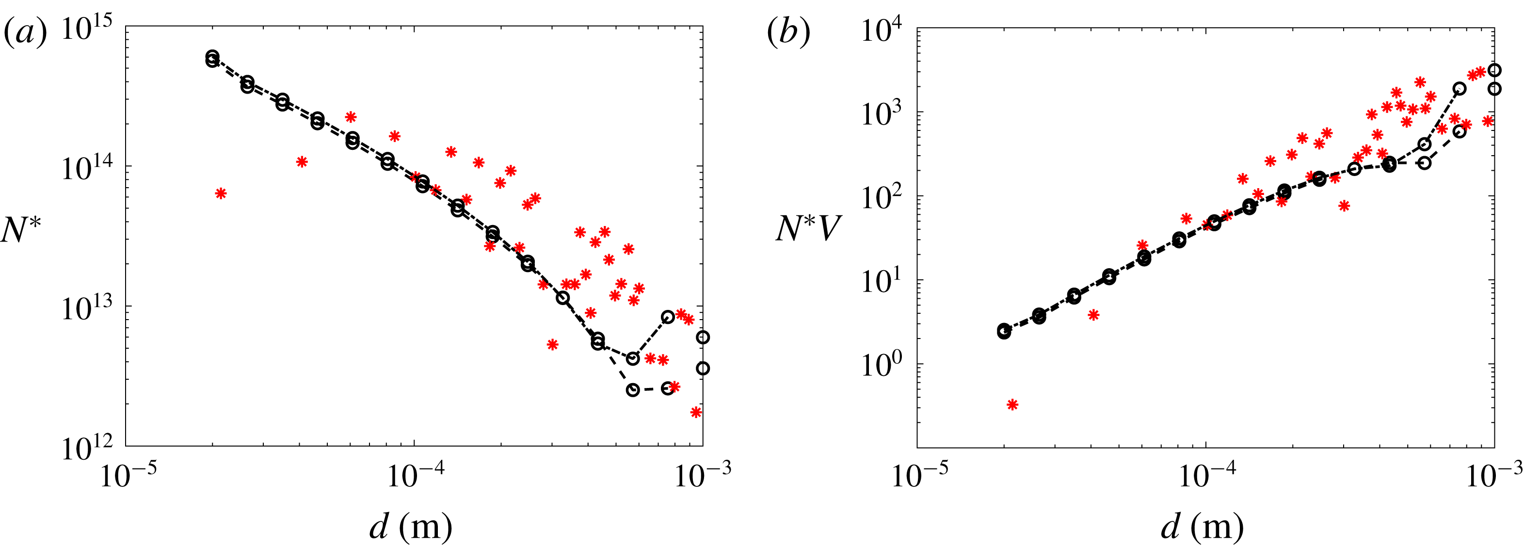
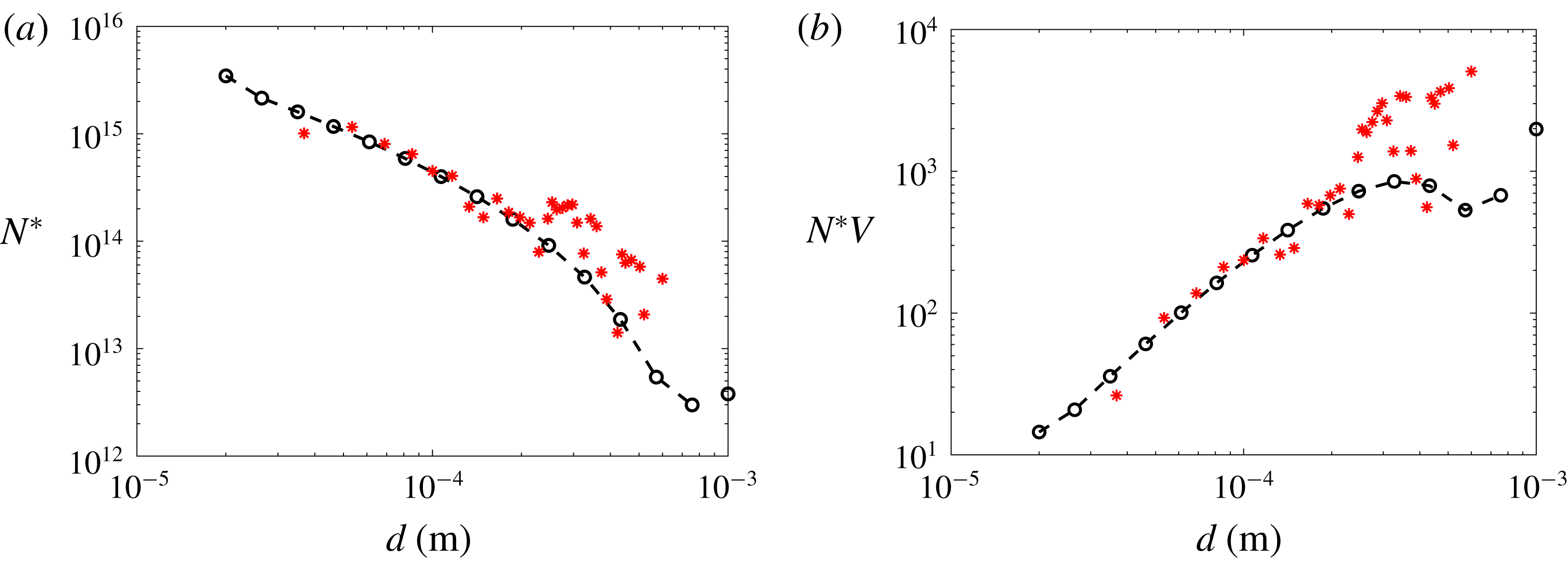
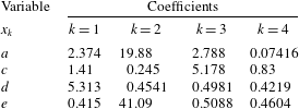
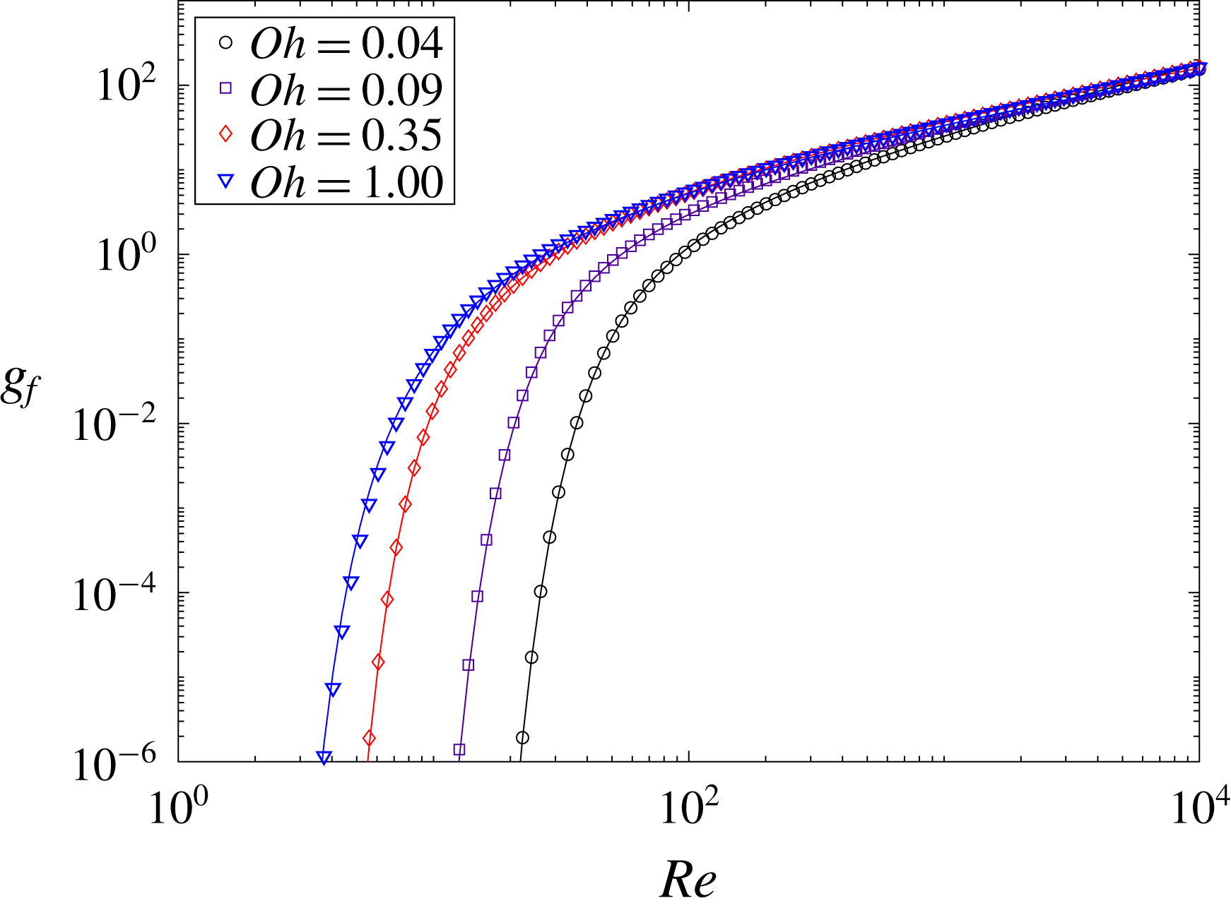
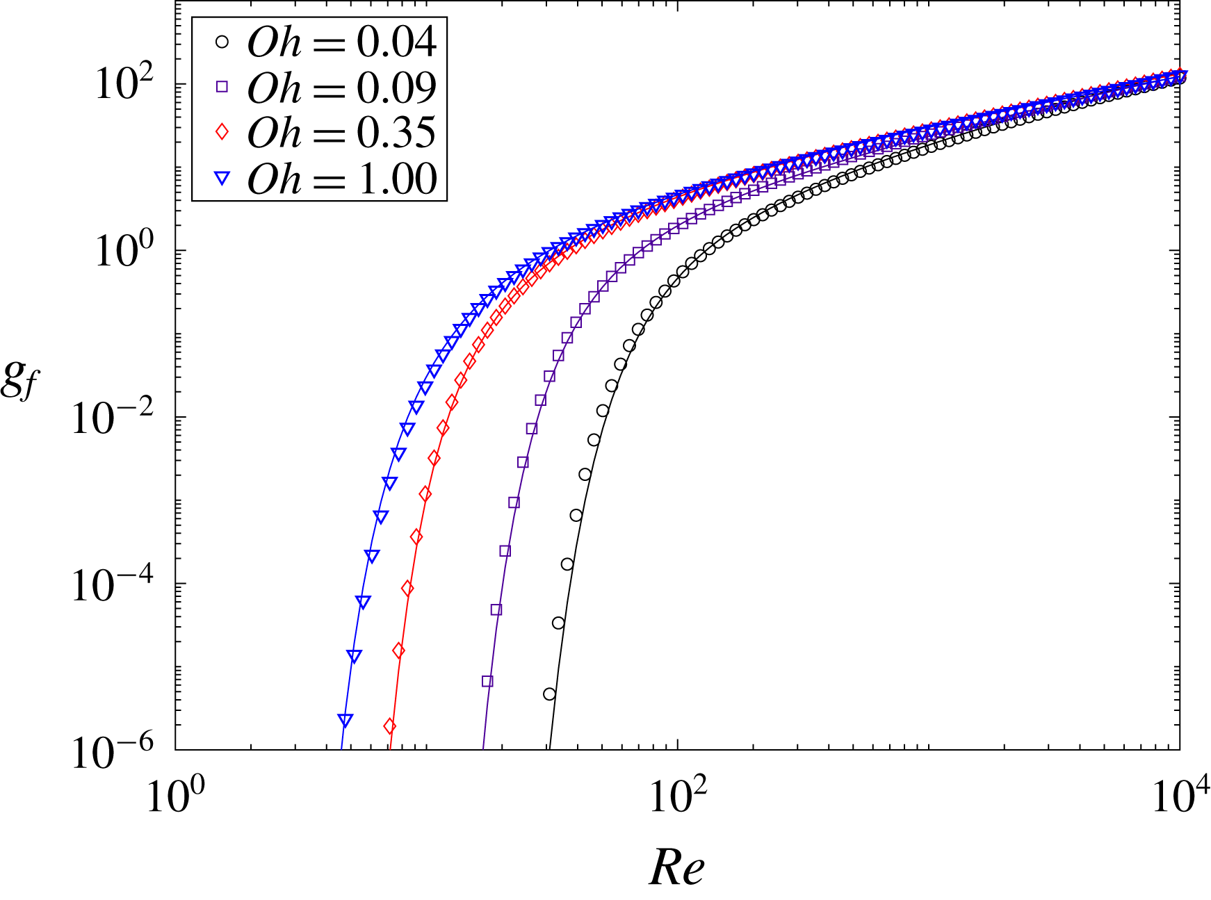
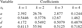
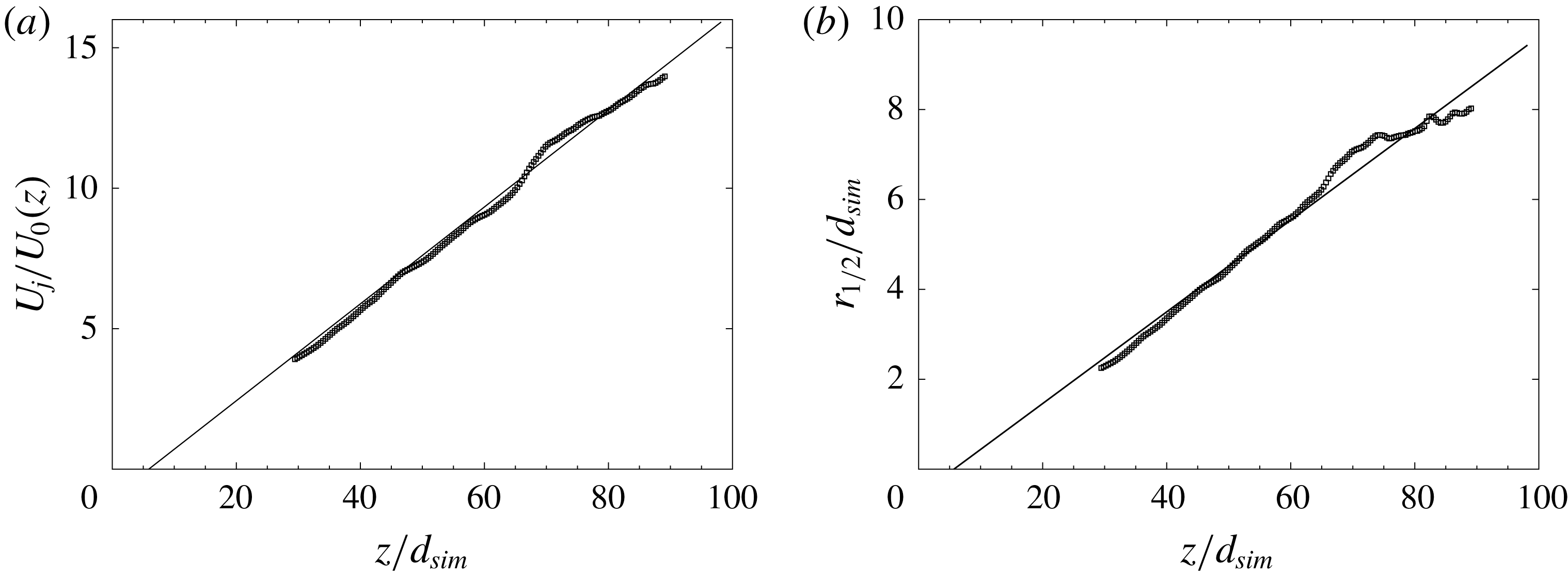
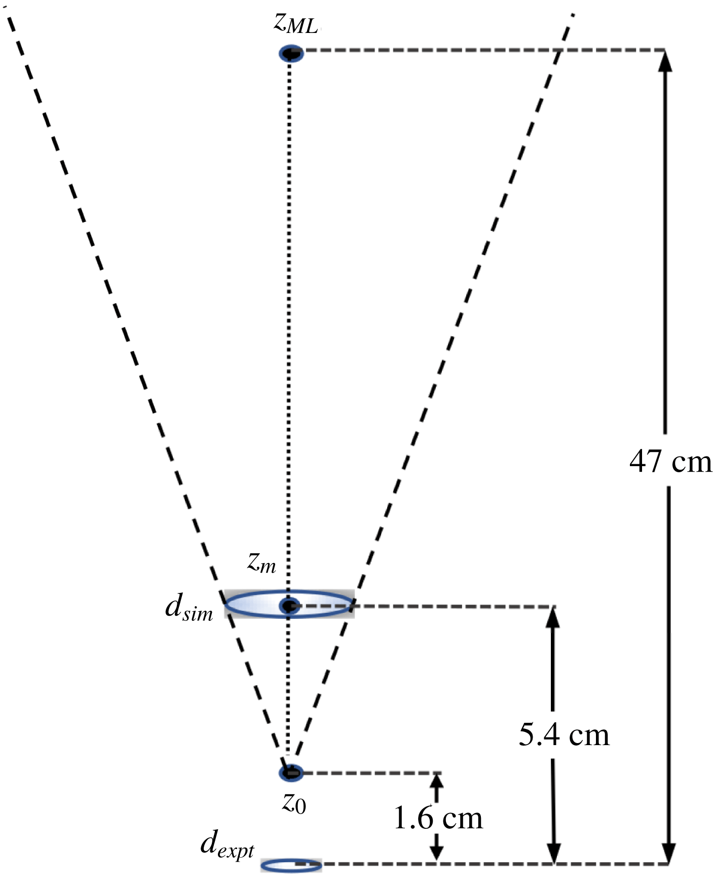
1 Introduction
An understanding of liquid droplet size distributions in turbulent flows is important in the context of numerous natural and engineering processes. For instance, knowledge of the droplet size distribution is important for predicting fate and transport of oil from an underwater spill (North et al. Reference North, Adams, Thessen, Schlag, He, Socolofsky, Masutani and Peckham2015; Nissanka & Yapa Reference Nissanka and Yapa2016). The size of oil droplets affects their rise velocity and can influence the entire plume’s transport characteristics in the ocean (Chen et al. Reference Chen, Yang, Meneveau and Chamecki2018). A review of recent developments in oil spill modelling can be found in Nissanka & Yapa (Reference Nissanka and Yapa2018). In combustion of fuel sprays the droplet size distribution plays an important role, determining atomization quality and spray combustion performance (Bossard & Peck Reference Bossard and Peck1996). The size distribution also plays a significant role in cloud dynamics, while also affecting the thermodynamic characteristics of the system (Liu et al. Reference Liu, You, Yang and Liu1995; Igel & van den Heever Reference Igel and van den Heever2016). Population balance equations (PBEs), initially formulated by Smoluchowski (Reference Smoluchowski1916) to study aggregation processes, are commonly used in many problems involving particulate systems with particles of many sizes. The basic formulation of PBEs has been extended by Hulburt & Katz (Reference Hulburt and Katz1964), Randolph (Reference Randolph1964) and Ramkrishna (Reference Ramkrishna1985) to include additional phenomena such as breakup, coalescence, nucleation, condensation, etc. PBEs can be classified into four main categories (Jakobsen Reference Jakobsen2014): method of moments, multi-class method, method of weighted residuals and stochastic methods. In this paper we use the multi-class formulation to study the evolution of polydisperse liquid droplets in a surrounding fluid. In this method the continuous size range is divided into a number of small contiguous subclasses, and the PBE is converted into a number of discretized transport equations for each class (bin). Methods such as the method of classes (Marchal et al. Reference Marchal, David, Klein and Villermaux1988), the fixed pivot method (Kumar & Ramakrishna Reference Kumar and Ramakrishna1996) and the cell average technique (Kumar et al. Reference Kumar, Peglow, Warnecke, Heinrich and Mörl2006) have been developed to discretize the PBE.
Coulaloglou & Tavlarides (Reference Coulaloglou and Tavlarides1977) were among the first to introduce a simple macroscopic formulation to study breakup and coalescence in an agitated liquid–liquid dispersion (droplets in a liquid), typically in a turbulent flow. Over the years, a considerable number of studies have been performed for steady-state size distributions in stirred vessels (e.g. Coulaloglou & Tavlarides Reference Coulaloglou and Tavlarides1977; Prince & Blanch Reference Prince and Blanch1990; Tsouris & Tavlarides Reference Tsouris and Tavlarides1994; Wang & Wang Reference Wang and Wang2007, among many others). These models used the average dissipation rate of turbulent kinetic energy to characterize the breakup, an approach well suited for use in Reynolds averaged Navier–Stokes (RANS)
 $k-\unicode[STIX]{x1D716}$
modelling, where the mean rate of dissipation
 $\langle \unicode[STIX]{x1D716}\rangle$
is a primary field variable available from the turbulence model. There have been several studies conducted in recent years that focus on predicting droplet size distribution either through models based on a RANS approach, or by using correlations for the mean size distribution (e.g. Bandara & Yapa Reference Bandara and Yapa2011; Brandvik et al.
Reference Brandvik, Johansen, Leirvik, Farooq and Daling2013; Johansen, Brandvik & Farooq Reference Johansen, Brandvik and Farooq2013; Zhao et al.
Reference Zhao, Boufadel, Socolofsky, Adams, King and Lee2014a
,Reference Zhao, Torlapati, Boufadel, King, Robinson and Lee
b
). More recently Pedel et al. (Reference Pedel, Thornock, Smith and Smith2014) used large eddy simulation (LES) coupled with an Eulerian solver for the droplet phase to predict droplet concentrations using the direct quadrature methods of moment (DQMOM). Neuber et al. (Reference Neuber, Kronenburg, Stein and Cleary2017) used an Eulerian LES coupled with a sparse Lagrangian droplet method to study aggregation and nucleation. Further work combining LES for the carrier flow with PBE for droplets can be found in Seubert et al. (Reference Seubert, Kronenburg, Stein, Ge and Cleary2012), Salehi, Cleary & Masri (Reference Salehi, Cleary and Masri2017) and Sewerin & Rigopoulos (Reference Sewerin and Rigopoulos2017), the latter of which used LES for the carrier phase coupled with a statistical Lagrangian approach for the droplets. However, Lagrangian methods can become expensive for large number of droplets. Even though limited to applications with relatively low volume fractions, Eulerian approaches can be advantageous since they are not limited by the number of droplets, as the distribution of droplets in each size range is described by a continuous concentration field. Yang et al. (Reference Yang, Chen, Socolofsky, Chamecki and Meneveau2016) used an Eulerian–Eulerian LES model to study bubble-driven buoyant plumes in a stably stratified quiescent fluid. They showed that the plume structure depended on the diameter of the droplets, but their LES only used a single bubble size in each simulation. Thus, there is interest in modelling plumes of droplets of many sizes and there is a need to extend LES to systems with polydisperse size distributions. There is little existing body of literature of combining LES with PBEs using the method of classes in the context of Eulerian descriptions of droplet concentration fields. The present paper is devoted to developing and testing such a tool.
The population balance equation is a transport equation that describes the evolution of the number density field representing the population of a type of particles due to advection, diffusion, breakup or coalescence. It can be written as
 $$\begin{eqnarray}\frac{\unicode[STIX]{x2202}n(d_{i},\boldsymbol{x},t)}{\unicode[STIX]{x2202}t}+\unicode[STIX]{x1D735}\boldsymbol{\cdot }[\boldsymbol{v}(d_{i},\boldsymbol{x},t)n(d_{i},\boldsymbol{x},t)]=S_{b,i}+S_{c,i},\end{eqnarray}$$
where
 $n(d_{i},\boldsymbol{x},t)$
is the number density of droplets of diameter
 $d_{i}$
,
 $\boldsymbol{v}(d_{i},\boldsymbol{x},t)$
is the droplet velocity,
 $S_{b,i}$
and
 $S_{c,i}$
are source terms for droplet breakup and coalescence affecting droplets of diameter
 $d_{i}$
(within bin
 $i$
), respectively. The divergence is calculated with respect to the spatial coordinate
 $\boldsymbol{x}$
. In this work we consider small dispersed phase volume fractions and neglect droplet coalescence (
 $S_{c,i}=0$
). Effects of evaporation, growth and aggregation have also been neglected in this work. The droplet concentration transport velocity
 $\boldsymbol{v}(d_{i},\boldsymbol{x},t)$
can be specified using the approach of Ferry & Balachandar (Reference Ferry and Balachandar2001) and Yang et al. (Reference Yang, Chen, Socolofsky, Chamecki and Meneveau2016) that includes effects of drag, buoyancy and relative acceleration (see § 4).
In order to close the problem, one needs a model for the source term
 $S_{b,i}$
. A number of models have been developed for breakup due to turbulent fluctuations. For a turbulent flow, breakup due to shearing-off processes and due to interfacial instability are often neglected. The turbulent fluctuations need to overcome the main resistive forces in the droplet, namely surface tension and viscosity. Prince & Blanch (Reference Prince and Blanch1990) and Tsouris & Tavlarides (Reference Tsouris and Tavlarides1994) treated the interaction between eddies and droplets similar to collisions between molecules in kinetic theory of gases. This allowed them to define a collision frequency based on the size of the eddy and droplet, and invoke a model for their typical relative velocity at that scale. The requirement for breakup in such a model is that the turbulent kinetic energy of the colliding eddy is greater than the potential energy associated with the resistive forces of the droplet. Skartlien, Sollum & Schumann (Reference Skartlien, Sollum and Schumann2013) and Zhao et al. (Reference Zhao, Torlapati, Boufadel, King, Robinson and Lee2014b
) extended the model of Prince & Blanch (Reference Prince and Blanch1990) and Tsouris & Tavlarides (Reference Tsouris and Tavlarides1994) to include the effect of viscosity in the resistive force. It should be noted that there are numerous other droplet breakup models in the literature based on criteria such as turbulent kinetic energy of the droplet being higher than a critical value (Coulaloglou & Tavlarides Reference Coulaloglou and Tavlarides1977; Chatzi & James Reference Chatzi and James1987), or the inertial force of colliding eddy exceeding the interfacial force of the smallest droplet (Lehr & Mewes Reference Lehr and Mewes1999), surface deformation and breakup due to turbulent stresses of surrounding fluid (Martínez-Bazán, Montañés & Lasheras Reference Martínez-Bazán, Montañés and Lasheras1999a
), to name a few.
In most of the previous formulations, the scale of the colliding droplets and eddies was assumed to be in the inertial range of turbulence. Hence Kolmogorov scaling for the inertial subrange was used to estimate the magnitude of eddy-velocity fluctuations at a particular scale. This precludes these models from being able to calculate the breakup frequency for droplets that fall in or near the viscous range, e.g. below
 $\unicode[STIX]{x1D702}$
up to approximately 15
 $\unicode[STIX]{x1D702}$
, where
 $\unicode[STIX]{x1D702}$
is the Kolmogorov length scale. A unified treatment is needed to extend these models to the entire spectrum of turbulence. Recently, Solsvik & Jakobsen (Reference Solsvik and Jakobsen2016) included the viscous range using a model energy spectrum (Pope Reference Pope2011) for the complete range of scales. Using a Fourier series transform, they derived the second-order structure function from this spectrum including the viscous range. The resulting expressions are somewhat complicated, owing to the particular functional form of the viscous cutoff in spectral space. However, a more direct approach and simpler expressions can already be found in the literature, based on the Batchelor blending function (Batchelor Reference Batchelor1951) written directly for the structure function in physical space. In this study, we adopt this particular physical space version for modelling the eddy-velocity fluctuations, since it affords more intuitive understanding and more efficient numerical evaluations of the model terms.
A significant number of experimental studies have been conducted in stirred tanks (Narsimhan, Ramkrishna & Gupta Reference Narsimhan, Ramkrishna and Gupta1980; Calabrese, Wang & Bryner Reference Calabrese, Wang and Bryner1986; Sathyagal, Ramkrishna & Narsimhan Reference Sathyagal, Ramkrishna and Narsimhan1996) and have been used to measure the droplet breakup frequency. However, it is challenging to relate the measured transient droplet size distributions to models due to the difficulty in characterizing the turbulence in stirred tanks which is highly anisotropic and spatially very heterogeneous. For instance, such flows contain highly localized high shear regions near the surface of the impeller blades and strong tip vortices shed by the blades.
There have been efforts to design suitable experiments in which the turbulence is well characterized. A well-known reference is that of Martínez-Bazán et al. (Reference Martínez-Bazán, Montañés and Lasheras1999a
) who designed and carried out a series of experiments where air bubbles were injected into a fully developed turbulent water jet. This ensured that the turbulence was well characterized and size distributions could be measured using non-intrusive optical techniques. Eastwood, Armi & Lasheras (Reference Eastwood, Armi and Lasheras2004) injected droplets of varying density, viscosity and interfacial tension into a fully developed water jet and tracked particle size distributions using digital image processing techniques. Brandvik et al. (Reference Brandvik, Johansen, Leirvik, Farooq and Daling2013) performed oil jet experiments in a very large cylindrical tank. They measured droplet size distributions using an in situ laser diffractometer. Murphy et al. (Reference Murphy, Xue, Sampath and Katz2016) used an oil jet in cross-flow to study the droplet breakup and resulting size distributions. Their experiment consisted of a nozzle supported by a carriage that was moved at a constant speed thus setting up a cross-flow. The size distribution was measured non-intrusively using in-line holographic techniques. Zhao et al. (Reference Zhao, Shaffer, Robinson, King, DAmbrose, Pan, Gao, Miller, Conmy and Boufadel2016) conducted a large-scale experiment of underwater oil release through a
 $25.4~\text{mm}$
pipe. They measured size distributions using two LISSTs (laser in situ scattering and transmissometry) in the range of
 $2.5{-}500~\unicode[STIX]{x03BC}\text{m}$
. Recently, Li et al. (Reference Li, Miller, Wang, Koley and Katz2017) studied the time evolution of subsurface oil droplets generated by breaking waves. They performed experiments for varying wave energy and surface tension and measured the generated size distribution using digital inline holography at two magnifications. Such experiments, where the flow is well characterized and the size distributions can be measured non-intrusively, are ideal to use as comparisons for models and we shall make use of such laboratory-scale oil droplet experimental data sets in the present work.
Over the recent decade, progress has been made in simulating two-phase flows using sufficiently fine spatial resolution to describe detailed deforming interfaces and thus capture the formation of droplets from instabilities of liquid sheets (Desjardins, Moureau & Pitsch Reference Desjardins, Moureau and Pitsch2008; Gorokhovski & Herrmann Reference Gorokhovski and Herrmann2008; Herrmann Reference Herrmann2010; Duret et al. Reference Duret, Luret, Reveillon, Menard, Berlemont and Demoulin2012; Herrmann Reference Herrmann2013). The aim is to, for example, simulate primary atomization and determine the resulting droplet size distributions. The LES tool described in the present work focuses on much coarser numerical meshes that cannot resolve such detailed dynamics and assume, for example, that the size distribution resulting from small-scale initial droplet formation processes is known.
The paper begins in § 2 with a description of the breakup model that is based on prior approaches used in RANS or integral models (Prince & Blanch Reference Prince and Blanch1990; Tsouris & Tavlarides Reference Tsouris and Tavlarides1994; Zhao et al. Reference Zhao, Torlapati, Boufadel, King, Robinson and Lee2014b ), extended here to include the correct scaling for droplets in the viscous range and adapted for applicability in LES. The modelling is focused on applications of LES where relatively coarse grids have to be employed and the small-scale details cannot be resolved. The model contains an undetermined multiplicative dimensionless parameter that is chosen by matching predictions of a simplified version of the model to an experiment in breaking waves, and we then verify its robustness under very different flow conditions (a round jet), as explained in § 3. An application to LES of a turbulent, droplet-laden jet in cross-flow is presented in § 4, focusing on the droplet breakup and transport occurring in regions away from the nozzle. In the present LES application, the nozzle details will not be resolved and thus the initial breakup mechanisms of oil into large droplets near the nozzle will be replaced by an appropriately chosen initial inflow condition of droplets of a given diameter. The focus of the study will be on comparing the size distributions far away from the nozzle with available experimental data, and to showcase the advantage of LES in being able to predict variability and intermittency of the size distribution and characteristic scales of the droplets. Conclusions are presented in § 5.
2 Droplet breakup model
The population balance equation described in (1.1), neglecting the effect of coalescence and written using the droplet size (diameter
 $d_{i}$
) as the internal coordinate, is given by
 $$\begin{eqnarray}\frac{\unicode[STIX]{x2202}n(d_{i},\boldsymbol{x},t)}{\unicode[STIX]{x2202}t}+\unicode[STIX]{x1D735}\boldsymbol{\cdot }[\boldsymbol{v}(d_{i},\boldsymbol{x},t)n(d_{i},\boldsymbol{x},t)]=S_{b}(d_{i},\boldsymbol{x},t),\end{eqnarray}$$
where
 $n(d_{i},\boldsymbol{x},t)$
is the number density of droplets in the
 $i$
th bin representing droplets of diameter around
 $d_{i}$
, at location
 $\boldsymbol{x}$
at time
 $t$
. The divergence is calculated with respect to the spatial coordinate
 $\boldsymbol{x}$
. The source term due to breakup is written according to Zhao et al. (Reference Zhao, Torlapati, Boufadel, King, Robinson and Lee2014b
),
 $$\begin{eqnarray}S_{b}(d_{i},\boldsymbol{x},t)=\mathop{\sum }_{j=i+1}^{n}P(d_{i},d_{j})g(d_{j},\boldsymbol{x},t)n(d_{j},\boldsymbol{x},t)-g(d_{i},\boldsymbol{x},t)n(d_{i},\boldsymbol{x},t).\end{eqnarray}$$
The first term on the right-hand side of (2.2) represents the birth of droplets of size
 $d_{i}$
due to the total contribution from breakups of larger droplets of diameter
 $d_{j}$
. The second term accounts for death of droplets of size
 $d_{i}$
due to breakup. The factor
 $P(d_{i},d_{j})$
is the probability of formation of a droplet of size
 $d_{i}$
due to the breakup of a parent droplet of size
 $d_{j}$
, and
 $g(d_{i},\boldsymbol{x},t)$
is the breakup frequency of a droplet of size
 $d_{i}$
(in bin
 $i$
). The breakup probability can be related to the probability density function
 $\unicode[STIX]{x1D6FD}(d_{i},d_{j})$
, i.e.
 $P(d_{i},d_{j})=\unicode[STIX]{x1D6FD}(d_{i},d_{j})\unicode[STIX]{x1D6FF}(d_{i})$
, where
 $\unicode[STIX]{x1D6FF}(d_{i})$
is the width of the bin centred at
 $d_{i}$
. Also note that the number density
 $n(d_{i},\boldsymbol{x},t)$
for discrete bins can be related to the more general continuous number density distribution function
 $n^{\ast }$
according to
 $$\begin{eqnarray}n(d_{i},\boldsymbol{x},t)=\int _{d_{i-1/2}}^{d_{i+1/2}}n^{\ast }(d,\boldsymbol{x},t)\,\text{d}(d),\end{eqnarray}$$
where
 $[d_{i+1/2}-d_{i-1/2}]$
is the
 $i$
th bin width. In order to solve (2.1), models are needed for the probability
 $P(d_{i},d_{j})$
and the breakup frequency
 $g(d_{i},\boldsymbol{x},t)$
.
2.1 Model for the breakup probability
Models for the breakup probability function
 $P(d_{i},d_{j})$
(or
 $\unicode[STIX]{x1D6FD}(d_{i},d_{j})$
), can broadly be classified as statistical, phenomenological or empirical (see Lasheras et al.
Reference Lasheras, Eastwood, Martínez-Bazán and Montaes2002; Liao & Lucas Reference Liao and Lucas2009). In this study we use the phenomenological model proposed by Tsouris & Tavlarides (Reference Tsouris and Tavlarides1994) that leads to a ‘U-shaped’ distribution. We keep in mind, however, that experiments for bubble breakup (Martínez-Bazán, Montañés & Lasheras Reference Martínez-Bazán, Montañés and Lasheras1999b
) have led to other possible shapes for
 $P(d_{i},d_{j})$
and that there remains considerable uncertainty about the best model to use. Here we proceed with the model of Tsouris & Tavlarides (Reference Tsouris and Tavlarides1994) because it is based on a relatively simple physical reasoning as shown below.
The breakup is considered to be binary, and
 $P(d_{i},d_{j})$
is formulated based on the formation energy required to form the daughter droplets of size
 $d_{i}$
and a complementary droplet to ensure volume conservation (Tsouris & Tavlarides Reference Tsouris and Tavlarides1994). The formation energy is proportional to the difference in initial and final surface areas according to
 $$\begin{eqnarray}E_{f}(d_{i},d_{j})=\unicode[STIX]{x03C0}\unicode[STIX]{x1D70E}[(d_{j}^{3}-d_{i}^{3})^{2/3}+d_{i}^{2}-d_{j}^{2}],\end{eqnarray}$$
where
 $\unicode[STIX]{x1D70E}$
is the interfacial tension between the dispersed and continuous phase. It can be shown using (2.4) that the breakup of a parent droplet into two equal size daughter droplets is a maximum energy process. Substituting
 $d_{i}=d_{j}/2^{1/3}$
in (2.4) we get a maximum formation energy equal to
 $$\begin{eqnarray}E_{f,max}=\unicode[STIX]{x03C0}\unicode[STIX]{x1D70E}d_{j}^{2}(2^{1/3}-1).\end{eqnarray}$$
Equation (2.4) is minimized when
 $d_{i}=0$
, that is no breakup of the parent droplet. To allow for breakup, a minimum diameter
 $d_{min}$
is specified and the corresponding surface formation energy is
 $$\begin{eqnarray}E_{f,min}=\unicode[STIX]{x03C0}\unicode[STIX]{x1D70E}[(d_{j}^{3}-d_{min}^{3})^{2/3}+d_{min}^{2}-d_{j}^{2}],\end{eqnarray}$$
where
 $d_{min}=1~\unicode[STIX]{x03BC}\text{m}$
in this study. Making the crucial assumption that the probability of breakup of a drop of size
 $d_{j}$
leading to a droplet of size such that it falls in a bin around
 $d_{i}$
decreases linearly with the required formation energy and remains within the bounds specified above, the discrete breakup probability
 $P(d_{i},d_{j})$
can be written as
 $$\begin{eqnarray}P(d_{i},d_{j})=\frac{[E_{f,min}+(E_{f,max}-E_{f}(d_{i},d_{j}))]}{\displaystyle \mathop{\sum }_{k=1}^{j-1}[E_{f,min}+(E_{f,max}-E_{f}(d_{k},d_{j}))]},\end{eqnarray}$$
where
 $E_{f}(d_{i},d_{j})$
is the surface formation energy defined in (2.4). Also, we assume that the bin sizes are logarithmically distributed. Thus (2.7) is meant to model the discrete probability that a particle of size
 $d_{j}$
breaks up into a particle inside a bin centred at
 $d_{i}$
with a width of
 $\unicode[STIX]{x1D6FF}(\log (d_{i}))$
, and its complement
 $d_{c}$
(to conserve volume). This distribution is U-shaped, with a minimum probability for the formation of two equally sized daughter droplets (when
 $E_{f}(d_{i},d_{j})=E_{f,max}$
which leads to a maximum of required energy), and probability maxima at the two ends (which have formation energy minima).
Martínez-Bazán et al. (Reference Rodríguez-rodríguez, Deane, Montañés and Lasheras2010) derived constraints that apply to the droplet size probability density function
 $\unicode[STIX]{x1D6FD}(d_{i},d_{j})$
for the breakup process to be volume conserving. The discrete probability of forming a droplet in bin
 $d_{i}$
must be equal to the probability of formation of the complement in bin
 $d_{c}$
. The discrete breakup probability in (2.7) conserves volume, since
 $P(d_{i},d_{j})=P(d_{c},d_{j})$
(we note that expressing this probability in terms of a universal density
 $\unicode[STIX]{x1D6FD}(d_{i},d_{j})$
presents further challenges (Martínez-Bazán et al.
Reference Rodríguez-rodríguez, Deane, Montañés and Lasheras2010) that are left for future analysis, while here we use the discrete version).
2.2 Model for breakup frequency
Modelling breakup based on encounter rates of turbulent eddies and their characteristic fluctuations with droplets of a certain size has been a popular method in the literature. The phenomenological model by Coulaloglou & Tavlarides (Reference Coulaloglou and Tavlarides1977) postulates that a droplet in a liquid–liquid dispersion breaks up when the kinetic energy transmitted from droplet–eddy collisions exceeds the surface energy. Many other papers have pursued this approach, mostly in the RANS context (e.g. Narsimhan, Gupta & Ramkrishna Reference Narsimhan, Gupta and Ramkrishna1979; Chatzi & James Reference Chatzi and James1987). Here we follow the approach of Prince & Blanch (Reference Prince and Blanch1990) and Tsouris & Tavlarides (Reference Tsouris and Tavlarides1994), where the droplet–eddy collisions are treated akin to the of collisions between molecules in kinetic theory of gases. The breakup frequency is computed as an integral over the product of a collision frequency and a breakup efficiency according to
 $$\begin{eqnarray}g(d_{i})=K\int _{0}^{d_{i}}\frac{\unicode[STIX]{x03C0}}{4}(d_{i}+d_{e})^{2}u_{e}(d_{e})\unicode[STIX]{x1D6FA}(d_{i},d_{e})\,\text{d}n_{e}(d_{e}).\end{eqnarray}$$
Here
 $d_{i}$
is the diameter of the droplet,
 $d_{e}$
is the eddy size,
 $n_{e}(d_{e})$
is the number density of eddies of size
 $d_{e}$
,
 $u_{e}(d_{e})$
is the characteristic fluctuation velocity of eddies of size
 $d_{e}$
(in a frame moving with the advection velocity caused by larger eddies),
 $\unicode[STIX]{x1D6FA}(d_{i},d_{e})$
is a breakup efficiency and the integral is evaluated over all eddies, up to the size of the droplet (i.e. for
 $d_{e}$
up to
 $d_{e}=d_{i}$
). A crucial assumption of the model is that eddies larger than the scale of the droplet are assumed to be only responsible for advection of the droplet, not contributing to collisions with the droplet that require relative velocity. One could develop a ‘smoother’ model in which the lack of deformation due to eddies larger than
 $d_{i}$
is included as an additional cutoff behaviour in the function
 $\unicode[STIX]{x1D6FA}(d_{i},d_{e})$
. Here we choose to include that cutoff behaviour by following earlier work (Tsouris & Tavlarides Reference Tsouris and Tavlarides1994; Luo & Svendsen Reference Luo and Svendsen1996) as a sharp cutoff, while lumping any possible dependencies on the exact cutoff scale into the unknown model parameter
 $K$
, expected to be of order unity.
The number density of eddies,
 $n_{e}(d_{e})$
, can be estimated from the energy spectrum (Azbel Reference Azbel1981; Tsouris & Tavlarides Reference Tsouris and Tavlarides1994; Solsvik, Maaß & Jakobsen Reference Solsvik, Maaß and Jakobsen2016), or more simply by assuming the eddies to be space filling, i.e.
 $n_{e}(d_{e})\propto d_{e}^{-3}$
. The latter argument leads to
 $\text{d}n_{e}(d_{e})=C_{1}d_{e}^{-4}\text{d}(d_{e})$
, where
 $C_{1}$
is a constant of order
 $1$
.
The eddy fluctuation velocity
 $u_{e}(r)$
written in terms of the two-point separation distance,
 $r$
, is assumed to be expressed based on the second-order longitudinal structure function
 $S_{2}(r)$
as
 $u_{e}(r)\sim [S_{2}(r)]^{1/2}$
. The structure function is defined according to (Pope Reference Pope2011),
 $$\begin{eqnarray}S_{2}(r)=\langle [u_{L}(\boldsymbol{x}+r\boldsymbol{e}_{L})-u_{L}(\boldsymbol{x})]^{2}\rangle ,\end{eqnarray}$$
where
 $u_{L}$
is the fluid velocity component in the direction of unit vector
 $\boldsymbol{e}_{L}$
and the angular brackets represent statistical averaging. In previous models (Tsouris & Tavlarides Reference Tsouris and Tavlarides1994; Bandara & Yapa Reference Bandara and Yapa2011; Zhao et al.
Reference Zhao, Torlapati, Boufadel, King, Robinson and Lee2014b
) a Kolmogorov scaling valid in the inertial range of turbulence was used for
 $S_{2}(r)$
, leading to
 $u_{e}(r)\sim (\unicode[STIX]{x1D716}r)^{1/3}$
. However, this expression cannot be used if the size of the droplet is near the viscous range of turbulence. In order to capture both inertial and viscous ranges, as well as a smooth transition between the two ranges, we use the approach of Batchelor (Reference Batchelor1951) with a blending function. In this approach, the structure function is given by
 $$\begin{eqnarray}S_{2}(r)=C_{2}\unicode[STIX]{x1D716}^{2/3}r^{2/3}\left[1+\left(\frac{r}{\unicode[STIX]{x1D6FE}_{2}\unicode[STIX]{x1D702}}\right)^{-2}\right]^{-2/3},\end{eqnarray}$$
where
 $\unicode[STIX]{x1D702}$
is the Kolmogorov length scale. We choose the usual value for the Kolmogorov coefficient
 $C_{2}\approx 2.1$
(Pope Reference Pope2011). The parameter
 $\unicode[STIX]{x1D6FE}_{2}=(15C_{2})^{3/4}\approx 13$
sets the cross-over scale between the inertial and viscous range. We note that while most prior models are for use in a RANS framework using the average energy dissipation,
 $\unicode[STIX]{x1D716}$
, in LES we can use a local value of the instantaneous rate of dissipation averaged over the grid scale, modelled as the subgrid-scale (SGS) dissipation rate. As a result, even though (2.10) is based on K41 theory (Kolmogorov Reference Kolmogorov1941), in LES we only assume K41 scaling for the scales below the grid scale while intermittency in the resolved range of scales can be explicitly computed, and its effects on breakup rates taken into account in the LES model.
The breakup efficiency
 $\unicode[STIX]{x1D6FA}(d_{i},d_{e})$
in (2.8) is the probability that a given eddy interacting with the droplet has sufficient energy to overcome the resistive forces in the system, namely surface tension and viscosity. It is assumed to be given by the usual formation potential in terms of an exponential (Coulaloglou & Tavlarides Reference Coulaloglou and Tavlarides1977; Prince & Blanch Reference Prince and Blanch1990)
 $$\begin{eqnarray}\unicode[STIX]{x1D6FA}(d_{i},d_{e})=\exp \left(-\frac{E_{\unicode[STIX]{x1D70E}}(d_{i})+E_{\unicode[STIX]{x1D708}}(d_{i})}{E_{e}(d_{e})}\right),\end{eqnarray}$$
where
 $E_{\unicode[STIX]{x1D70E}}(d_{i})$
is resistive energy associated with a droplet of size
 $d_{i}$
due to surface tension,
 $E_{\unicode[STIX]{x1D708}}(d_{i})$
is the viscous resistive energy and
 $E_{e}(d_{e})$
is the kinetic energy of the turbulent eddy at scale
 $d_{e}$
. The resistive surface tension energy
 $E_{\unicode[STIX]{x1D70E}}$
is defined as the integral of the formation energy
 $E_{f}(d^{\prime },d_{i})$
multiplied by a measure of the breakup probability (see (2.7)):
 $$\begin{eqnarray}E_{\unicode[STIX]{x1D70E}}(d_{i})=\int _{0}^{d_{i}}c[E_{f,min}+(E_{f,max}-E_{f}(d^{\prime },d_{i}))]E_{f}(d^{\prime },d_{i})\,\text{d}(d^{\prime }),\end{eqnarray}$$
where
 $c$
is a normalization constant so that the integral of the probability between 0 and
 $d_{i}$
is unity. Using (2.4), changing the integration to
 $\unicode[STIX]{x1D709}^{\prime }=d^{\prime }/d_{i}$
and evaluating the integral numerically, we obtain
 $$\begin{eqnarray}E_{\unicode[STIX]{x1D70E}}(d_{i})=0.0702\unicode[STIX]{x03C0}\unicode[STIX]{x1D70E}d_{i}^{2},\end{eqnarray}$$
where
 $\unicode[STIX]{x1D70E}$
is the surface tension of the droplet. The viscous resistive energy of the droplet at steady state can be expressed as (Calabrese et al.
Reference Calabrese, Wang and Bryner1986; Skartlien et al.
Reference Skartlien, Sollum and Schumann2013; Zhao et al.
Reference Zhao, Torlapati, Boufadel, King, Robinson and Lee2014b
)
 $$\begin{eqnarray}E_{\unicode[STIX]{x1D708}}(d_{i})=\unicode[STIX]{x1D6FC}\frac{\unicode[STIX]{x03C0}}{6}\unicode[STIX]{x1D716}^{1/3}d_{i}^{7/3}\unicode[STIX]{x1D707}_{d}\sqrt{\frac{\unicode[STIX]{x1D70C}_{c}}{\unicode[STIX]{x1D70C}_{d}}},\end{eqnarray}$$
where
 $\unicode[STIX]{x1D6FC}\approx 2$
,
 $\unicode[STIX]{x1D70C}_{c}$
and
 $\unicode[STIX]{x1D70C}_{d}$
are the carrier and droplet phase density, and
 $\unicode[STIX]{x1D707}_{d}$
is the dynamic viscosity of the dispersed droplet phase. For
 $E_{e}(d_{e})$
, the kinetic energy of the turbulent eddy, we use the longitudinal structure function
 $S_{2}$
, defined in (2.10) applied to all three coordinate directions for the eddy fluctuation velocity,
 $u_{e}$
. Assuming the volume of the eddy to be equal to that of a sphere, with density equal to the carrier phase density, the total energy contained in an eddy can be written as
 $$\begin{eqnarray}E_{e}(d_{e})=\frac{3}{2}\left(\frac{\unicode[STIX]{x03C0}}{6}\unicode[STIX]{x1D70C}_{c}d_{e}^{3}\right)S_{2}(d_{e}).\end{eqnarray}$$
In order to formulate a parameterization for the breakup frequency, here we identify the important non-dimensional numbers of the system. The breakup frequency can be rewritten as a function of the Reynolds number (
 $Re_{i}$
) based on droplet diameter and a velocity scale defined as
 $u_{d_{i}}=(\unicode[STIX]{x1D716}d_{i})^{1/3}$
, the Ohnesorge number (
 $Oh_{i}$
) of the dispersed phase controlling the relative importance of viscosity to surface tension of the droplet, and the density and viscosity ratio of droplet to carrier flow fluid. These non-dimensional numbers are defined below,
 $$\begin{eqnarray}Re_{i}=\frac{\unicode[STIX]{x1D716}^{1/3}d_{i}^{4/3}}{\unicode[STIX]{x1D708}};\quad Oh_{i}=\frac{\unicode[STIX]{x1D707}_{d}}{\sqrt{\unicode[STIX]{x1D70C}_{d}\unicode[STIX]{x1D70E}d_{i}}};\quad \unicode[STIX]{x1D6E4}=\frac{\unicode[STIX]{x1D707}_{d}}{\unicode[STIX]{x1D707}_{c}}\left(\frac{\unicode[STIX]{x1D70C}_{c}}{\unicode[STIX]{x1D70C}_{d}}\right)^{1/2}.\end{eqnarray}$$
After some manipulation, equation (2.8) can be rewritten as
 $$\begin{eqnarray}g_{i}=K^{\ast }\frac{1}{\unicode[STIX]{x1D70F}_{b,i}}\int _{0}^{1}r_{e}^{-11/3}(r_{e}+1)^{2}\left(1+\left(\frac{r_{e}Re_{i}^{3/4}}{\unicode[STIX]{x1D6FE}_{2}}\right)^{-2}\right)^{-1/3}\unicode[STIX]{x1D6FA}(Oh_{i},Re_{i},\unicode[STIX]{x1D6E4};r_{e})\,\text{d}r_{e},\end{eqnarray}$$
where,
 $r_{e}=d_{e}/d_{i}$
is the eddy size normalized by the droplet diameter,
 $\unicode[STIX]{x1D70F}_{b,i}=\unicode[STIX]{x1D716}^{-1/3}d_{i}^{2/3}$
is the breakup time scale for an eddy of size equal to that of the droplet as if it were in the inertial range (it does not have to be) and
 $\unicode[STIX]{x1D6FA}(Oh,Re,\unicode[STIX]{x1D6E4};r_{e})$
is the non-dimensional breakup probability,
 $$\begin{eqnarray}\unicode[STIX]{x1D6FA}(Oh,Re,\unicode[STIX]{x1D6E4};r_{e})=\exp \left(-\frac{\unicode[STIX]{x1D6E4}f_{2}}{Re}\left[1+\left(\frac{r_{e}Re^{3/4}}{\unicode[STIX]{x1D6FE}_{2}}\right)^{-2}\right]^{2/3}r_{e}^{-11/3}\right),\end{eqnarray}$$
where
 $$\begin{eqnarray}f_{2}=0.14\frac{\unicode[STIX]{x1D6E4}}{ReOh^{2}}+0.583.\end{eqnarray}$$
All the non-dimensional prefactors appearing when rewriting (2.8) have been absorbed into
 $K^{\ast }$
. Equation (2.17) provides a frequency for droplet breakup that depends on
 $Re_{i}$
,
 $Oh_{i}$
and
 $\unicode[STIX]{x1D6E4}$
. Note that if we had only considered an inertial-range scaling for the eddy fluctuation velocity, we can combine
 $Re$
and
 $Oh$
into a Weber number, defined as
 $We=Re^{2}~Oh^{2}$
. The breakup frequency would then only depend on
 $We$
and
 $\unicode[STIX]{x1D6E4}$
. The integral represents a correction to the frequency calculated by solely considering an eddy equal to the size of the droplet, by evaluating the effect of collisions of eddies smaller than the droplet. If
 $d_{i}$
falls in the viscous range, the integral cancels the inertial-range scaling assumed by the prefactor
 $\unicode[STIX]{x1D70F}_{b,i}=\unicode[STIX]{x1D716}^{-1/3}d_{i}^{2/3}$
so that this situation is also accounted for. We note that the value of the integral
 $g_{i}\unicode[STIX]{x1D70F}_{b,i}/K^{\ast }$
in (2.17) will inevitably depend on the assumed maximum eddy size interacting with the droplet, which is currently taken to be exactly the droplet size
 $d_{i}$
. However, if one were to take a different upper integration limit (still of order
 $d_{i}$
but not exactly
 $d_{i}$
), the breakup frequency may not change much since the modified value of the integral will be largely (but not exactly) cancelled when fitting the prefactor
 $K$
to data. This behaviour is demonstrated in the next section.
In LES,
 $g_{i}$
needs to be evaluated on every grid point and timestep, depending on the local Reynolds number
 $Re_{i}$
and the local rate of dissipation. Evaluating numerically the integral in (2.17) at every timestep and grid point would be prohibitive in practice. Hence, we develop an empirical fit to prior numerical integrations. The speedup obtained from the fits is discussed in appendix A. We develop the parameterization for a wide range of Reynolds and Ohnesorge numbers, for a fixed value of
 $\unicode[STIX]{x1D6E4}$
. We define
 $g_{f}(Re,Oh,\unicode[STIX]{x1D6E4})$
as the integral in (2.17), i.e.
 $g_{f}(Re,Oh,\unicode[STIX]{x1D6E4})=g_{i}(Re_{i},Oh_{i},\unicode[STIX]{x1D6E4})\,\unicode[STIX]{x1D70F}_{b,i}/K^{\ast }$
, and evaluate it numerically for a range of
 $Re$
and
 $Oh$
values for a fixed
 $\unicode[STIX]{x1D6E4}$
. Then, a fit can be developed in the following form,
 $$\begin{eqnarray}\log _{10}(g_{f})=ax^{b}+cx^{d}-e,\end{eqnarray}$$
where
 $x=\log _{10}Re$
, and
 $a,b,c,d,e$
are functions of
 $Oh$
. Further details of the functional form of the coefficients are provided in appendix A. The final model for the breakup frequency (for a given value of
 $\unicode[STIX]{x1D6E4}$
) thus has the form
 $$\begin{eqnarray}\left.\begin{array}{@{}c@{}}\displaystyle g_{i}(Re_{i},Oh_{i};\unicode[STIX]{x1D6E4})=\frac{K^{\ast }}{\unicode[STIX]{x1D70F}_{b,i}}10^{G(Re_{i},Oh_{i})},\\ G(Re_{i},Oh_{i})=a[\log _{10}(Re_{i})]^{b}+c[\log _{10}(Re_{i})]^{d}-e,\end{array}\right\}\end{eqnarray}$$
where the fits for parameters
 $a$
–
 $e$
as functions of
 $Oh$
are provided in appendix A for a few representative values of
 $\unicode[STIX]{x1D6E4}$
.
The breakup frequency model is thus complete except for the prefactor
 $K^{\ast }$
appearing in (2.17). Its value is obtained by fitting results from an experiment (see next section), and the fitted value will then be used subsequently for comparisons with other data and for future applications.
3 Determining the value of
 $K^{\ast }$

3.1 Wave breaking experiment of Li et al. (Reference Li, Miller, Wang, Koley and Katz2017)
In order to fit a specific value for the parameter
 $K^{\ast }$
we use the data of a breaking wave experiment from Li et al. (Reference Li, Miller, Wang, Koley and Katz2017). The experiments were performed in an acrylic tank
 $6~\text{m}$
long,
 $0.6~\text{m}$
deep and
 $0.3~\text{m}$
wide. Breaking waves were generated mechanically using a piston-type wave maker consisting of a vertical plate that extends over the entire tank cross-section. The tank was filled with water up to a height of
 $0.25~\text{m}$
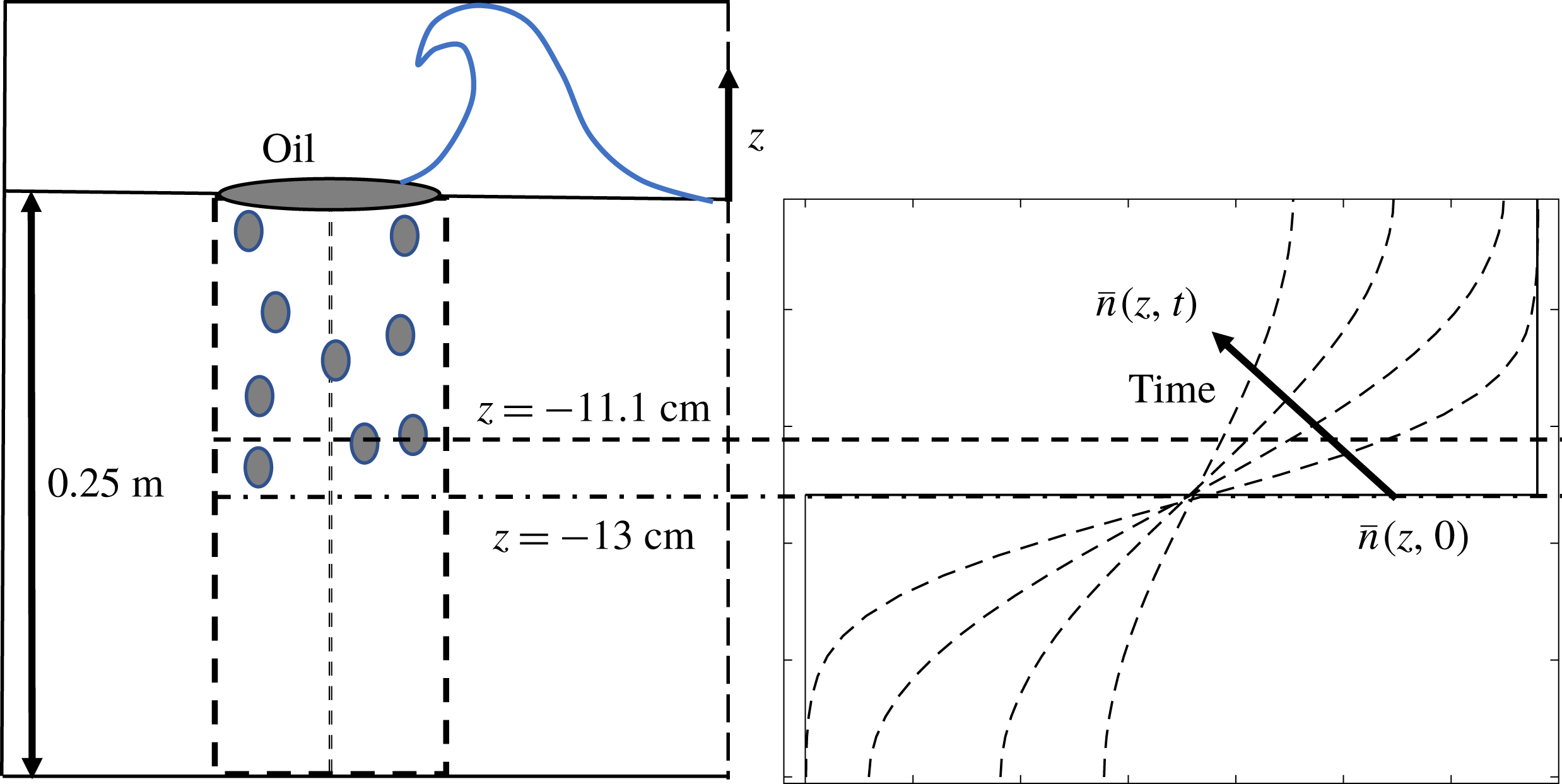
. The wave height and characteristics were controlled by varying the frequency and stroke of the vertical plate. Oil was placed on a patch at the surface. The wave impingement and subsequent breakup processes were recorded using 3 high-speed cameras. The droplet size distribution was measured using digital inline holography. A sketch of the set-up is depicted in figure 1. The oil patch on the surface was broken up into droplets by the plunging wave. The size distribution generated due to this process was recorded at a depth of
 $11.1~\text{cm}$
from the free surface. A simplified sketch of the evolution of the concentration of a particular droplet size is shown in figure 1(b).
(a) Sketch of the wave breaking experiment of Li et al. (Reference Li, Miller, Wang, Koley and Katz2017). (b) Schematic dependence of
 $\overline{n}_{i}(z,t)$
on time and height for a particular droplet size, starting from a step-function initial condition that is assumed to be well mixed initially down to a depth of 13 cm below the surface and having zero concentration below. At increasing times, turbulent diffusion smooths the step and droplets rise towards the surface at different speeds depending on their size. The dotted horizontal line at
 $z=-11.1$
cm is where the experimental data are available.

As shown by Li et al. (Reference Li, Miller, Wang, Koley and Katz2017), the time evolution of the droplet size distribution at the measurement location could be represented well by a simple model that includes the effects of turbulent diffusion and droplet buoyancy only. Since the dissipation rate was quite low at the measurement location, Li et al. (Reference Li, Miller, Wang, Koley and Katz2017) neglected the effect of droplet breakup in their model. Consequently, for the case of crude oil with dispersants, the model under-predicted the number of smaller size droplets generated. This is due to the fact that with the effect of dispersants, the surface tension of the oil droplets was significantly lowered, resulting in droplet breakup despite of the weak turbulent dissipation rate. The Weber number (
 $We=2\unicode[STIX]{x1D70C}(\unicode[STIX]{x1D716}d)^{2/3}d/\unicode[STIX]{x1D70E}$
) based on the droplet diameter for the case with dispersants is approximately
 $We=3$
, confirming that the effects of droplet breakup are important. Our goal is to expand the model of Li et al. (Reference Li, Miller, Wang, Koley and Katz2017) by including breakup and select a value of
 $K^{\ast }$
that can achieve improved agreement with their experimental data.
Adding the effect of breakup and following Li et al. (Reference Li, Miller, Wang, Koley and Katz2017) in considering only vertical diffusion and droplet rise velocity, the ensemble-averaged number density
 $\bar{n}_{i}(z,t)$
for a droplet of size
 $d_{i}$
obeys
 $$\begin{eqnarray}\frac{\unicode[STIX]{x2202}\bar{n}_{i}(z,t)}{\unicode[STIX]{x2202}t}+w_{r}(d_{i})\frac{\unicode[STIX]{x2202}\bar{n}_{i}(z,t)}{\unicode[STIX]{x2202}z}=D(t)\frac{\unicode[STIX]{x2202}^{2}\bar{n}_{i}}{\unicode[STIX]{x2202}z^{2}}+\mathop{\sum }_{j=i+1}^{n}P(d_{i},d_{j})g(d_{j})\bar{n}_{j}(z,t)-g(d_{i})\bar{n}_{i}(z,t),\end{eqnarray}$$
where
 $z$
is the vertical coordinate,
 $w_{r}(d_{i})$
is the buoyancy-induced rise velocity of droplets of size
 $d_{i}$
and
 $D(t)$
is the turbulent diffusion coefficient. The daughter droplet probability function
 $P(d_{i},d_{j})$
and the breakup frequency
 $g$
are evaluated following the model presented in § 2. The droplet rise velocity is calculated as a balance between the drag and buoyancy force acting on a droplet.
 $$\begin{eqnarray}w_{r}(d)=\left\{\begin{array}{@{}ll@{}}w_{r,S}\quad & \text{if }Re_{d}<0.2,\\ w_{r,S}(1+0.15Re_{d}^{0.687})^{-1},\quad & 0.2<Re_{d}<750,\end{array}\right.\end{eqnarray}$$
where
 $$\begin{eqnarray}w_{r,S}=\frac{(\unicode[STIX]{x1D70C}_{0}-\unicode[STIX]{x1D70C}_{d})g~d^{2}}{18\unicode[STIX]{x1D707}_{f}},\end{eqnarray}$$
and
 $Re_{d}=\unicode[STIX]{x1D70C}_{0}w_{r}d/\unicode[STIX]{x1D707}_{f}$
is the droplet rise velocity Reynolds number (not to be confused with the eddy Reynolds number
 $Re_{i}$
used to express the breakup frequency). The time-dependent diffusion coefficient can be estimated using
 $D(t)=k_{D}u^{\prime }(t)L(t)$
, where
 $u^{\prime }(t)$
is the time-dependent turbulent fluctuation (root-mean-square) velocity as measured in the experiment and
 $L(t)$
is the corresponding integral length scale, also measured. The constant
 $k_{D}$
is known to be between
 $0.23$
and
 $0.6$
for diffusion of droplets in isotropic turbulence (Sato & Yamamoto Reference Sato and Yamamoto1987; Gopalan, Malkiel & Katz Reference Gopalan, Malkiel and Katz2008). We chose a value of
 $k_{D}=0.3$
in accordance with Li et al. (Reference Li, Miller, Wang, Koley and Katz2017) for this study. Li et al. (Reference Li, Miller, Wang, Koley and Katz2017) fit the values of
 $u^{\prime }(t)$
(in
 $\text{m}~\text{s}^{-1}$
) and
 $\unicode[STIX]{x1D716}$
(in
 $\text{m}^{2}~\text{s}^{-3}$
) with a power law in time. The data can be represented as
 $(\unicode[STIX]{x1D716}/\unicode[STIX]{x1D716}_{0})=(t/t_{0})^{p}$
and
 $(u^{\prime }/u_{0}^{\prime })=(t/t_{0})^{q}$
where
 $\unicode[STIX]{x1D716}_{0}\approx 0.2~\text{m}^{2}~\text{s}^{-3}$
,
 $u_{0}^{\prime }\approx 0.2~\text{m}~\text{s}^{-1}$
and
 $t_{0}\approx 7~\text{s}$
. The exponents
 $p$
and
 $q$
can be related by
 $p=2q-1$
, and the data were fitted with
 $q=-0.89$
(Li et al.
Reference Li, Miller, Wang, Koley and Katz2017). The integral length scale
 $L(t)$
is then calculated as
 $u^{\prime }(t)^{3}/\unicode[STIX]{x1D716}(t)$
.
We solve (3.1) numerically for the number density of the oil droplets. We discretize the size range into
 $N_{d}=70$
bins and assume that at the initial time all the concentrations are spatially homogeneous in the
 $z$
direction down to an initial intrusion depth of
 $z=13$
cm (see figure 1). The concentration equations are solved for each droplet size using a second-order Crank–Nicholson temporal discretization method. The boundary condition at the bottom of the domain, at
 $z=-25~\text{cm}$
is that of no flux, i.e.
 $\bar{n}_{i}w_{r}-D(\unicode[STIX]{x2202}\bar{n}_{i}/\unicode[STIX]{x2202}z)=0$
. A Neumann boundary condition is applied at the top surface, i.e.
 $(\unicode[STIX]{x2202}\bar{n}_{i}/\unicode[STIX]{x2202}z)=0$
. We initialize the concentration of each diameter bin with the measured concentration at
 $z=-11.1~\text{cm}$
which was recorded after
 $5~\text{s}$
of impingement in the experiment. We integrate the model using different values of
 $K^{\ast }$
ranging from
 $0$
to
 $1$
.
Time evolution of the droplet size distribution for two values of
 $K^{\ast }$
, at the measurement location. The symbols correspond to the experimental data,
 $t=5~\text{s}$
(○) represents the initial condition where experiment and simulation are matched,
 $t=15~\text{s}$
(*),
 $t=35~\text{s}$
(▫),
 $t=55~\text{s}$
(♢), while the lines correspond to the simulation,
 $t=15~\text{s}$
(- - -),
 $t=35~\text{s}$
(-
 $\cdot$
-
 $\cdot$
) and
 $t=55~\text{s}$
(
 $\cdots$
). The green stars
 $(\star )$
in (a) correspond to the size distribution at
 $t=55~\text{s}$
using
 $N_{d}=15$
bins.

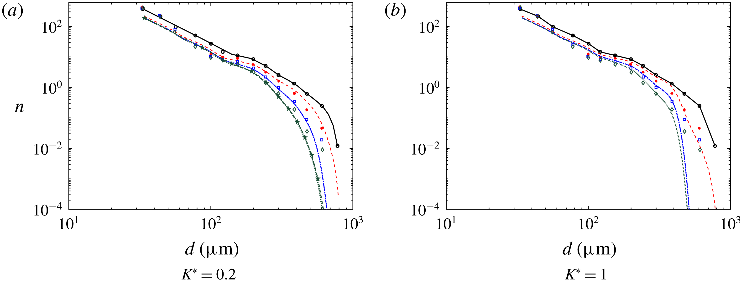
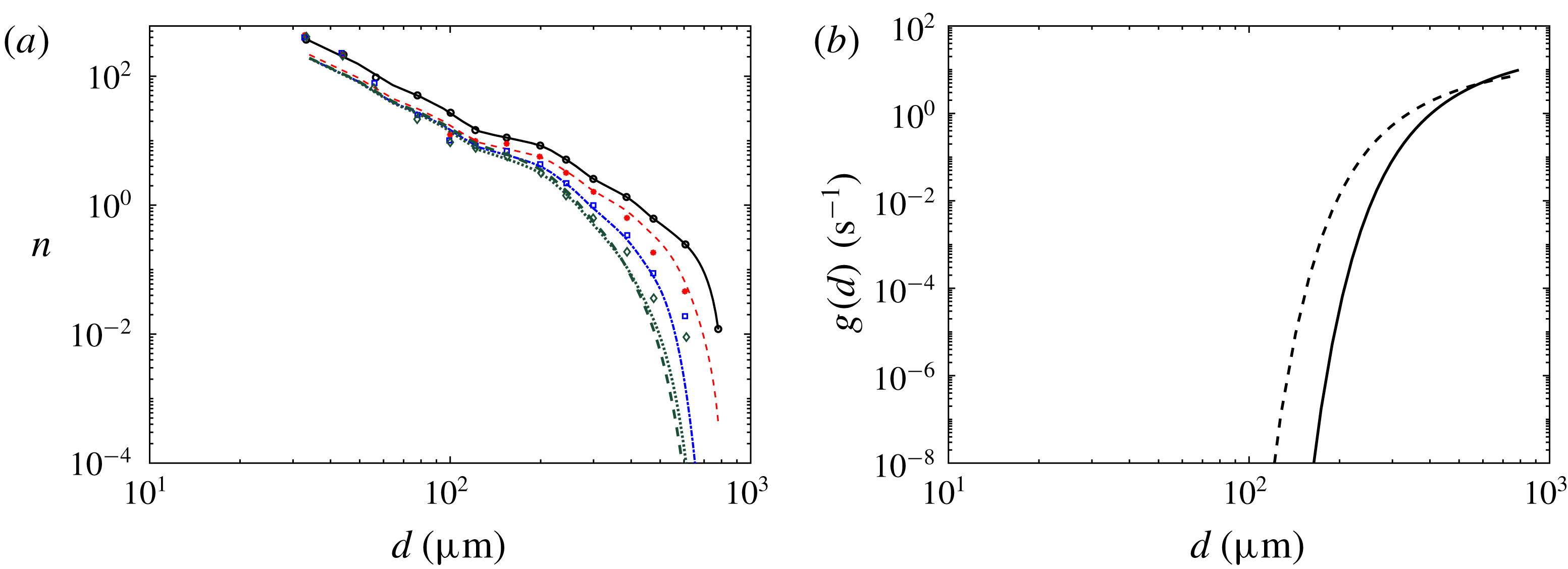
In figure 2 we compare the modelled size distributions (lines) to the experimental data (symbols) at various times, for
 $K^{\ast }=0.2$
and
 $K^{\ast }=1$
, at the measurement location
 $z=-11.1~\text{cm}$
. Since the initial condition (black circles in figure 2) already includes the effects of significant initial breakup of the oil, a size distribution is already formed. Since the energy dissipation at the point of measurement,
 $z=-11.1~\text{cm}$
is relatively low, the rate of further breakup is not very large and thus the effect of
 $K^{\ast }$
in the model is subtle. Nevertheless, close inspection shows that there is too much breakup effect for the large droplets for
 $K^{\ast }=1$
, as we can see that the number density of the larger droplets is lower than the experimental data, especially for later times. Qualitatively, it appears that
 $K^{\ast }=0.2$
captures the distribution slightly better, for both small and large droplets at the various time instants. We also calculate the size distribution in (3.1) using a coarser discretization of
 $N_{d}=15$
bins. The resulting number density
 $\bar{n}$
is shown in figure 2(a) at
 $t=55~\text{s}$
using green stars. We see that for this coarser resolution there is a good agreement with the
 $N_{d}=70$
case.
In order to make a quantitative comparison we define an error measure
 ${\mathcal{E}}$
as the integrated squared difference between the logarithmic experimental and modelled size distributions. The error is calculated for each droplet size, and integrated over all bins (the bin size varies logarithmically),
 $$\begin{eqnarray}{\mathcal{E}}=\mathop{\left\langle \mathop{\sum }_{i_{min}}^{i_{max}}[\log _{10}(\bar{n}_{expt}(d_{i}))-\log _{10}(\bar{n}_{mod}(d_{i}))]^{2}\frac{\unicode[STIX]{x1D6FF}d_{i}}{d_{i}}\right\rangle }\nolimits_{\!t},\end{eqnarray}$$
where
 $\unicode[STIX]{x1D6FF}d_{i}$
is the bin width,
 $\bar{n}_{expt}$
refers to the experimental size distribution and
 $\bar{n}_{mod}$
is the modelled one. The maximum diameter at which the experimental data are reported is
 $d\approx 500~\unicode[STIX]{x03BC}\text{m}$
. Therefore, we select
 $i_{max}=52$
corresponding to
 $d=505~\unicode[STIX]{x03BC}\text{m}$
. And we use
 $i_{min}=4$
corresponding to
 $d=86~\unicode[STIX]{x03BC}\text{m}$
. The error is averaged over the three available times,
 $t=15~\text{s}$
,
 $35~\text{s}$
and
 $55~\text{s}$
.
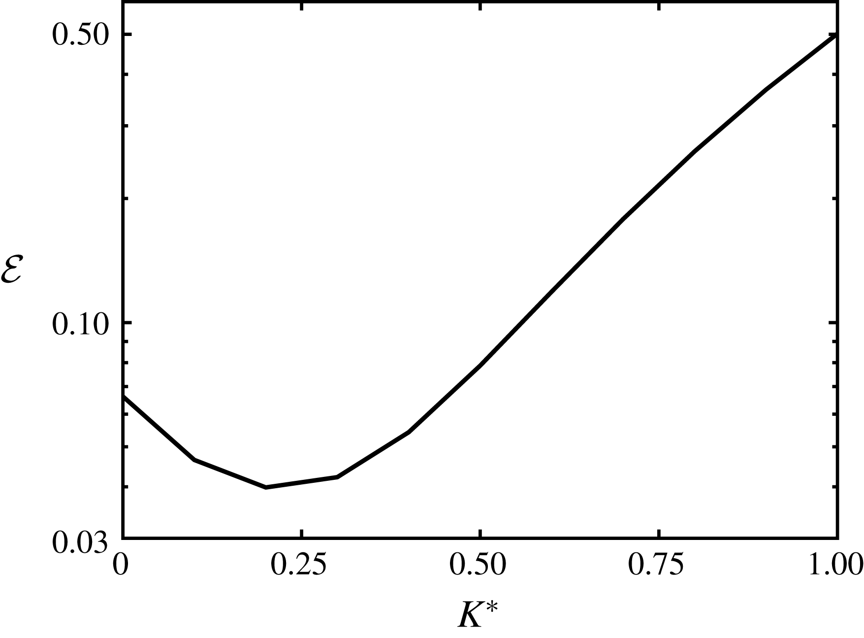
Average square error between predicted and measured logarithms of number densities averaged over three times during the evolution, at the measurement position, as a function of the breakup constant
 $K^{\ast }$
assumed in the model.

As can be seen from figure 3, the absolute value of the error is smallest at
 $K^{\ast }\approx 0.2$
and hence this value is chosen as the fitted parameter for future applications of the model. Note that
 $K^{\ast }=0$
corresponds to the case without breakup. We can see from figure 3 that the error is larger, showing the improved agreement when including the breakup term in the model.
As stated earlier in the text, previous breakup models use an inertial-range scaling for the eddy fluctuation velocity for the entire range of scales,
 $$\begin{eqnarray}u_{e}^{2}=2.1(\unicode[STIX]{x1D716}d_{e})^{2/3}.\end{eqnarray}$$
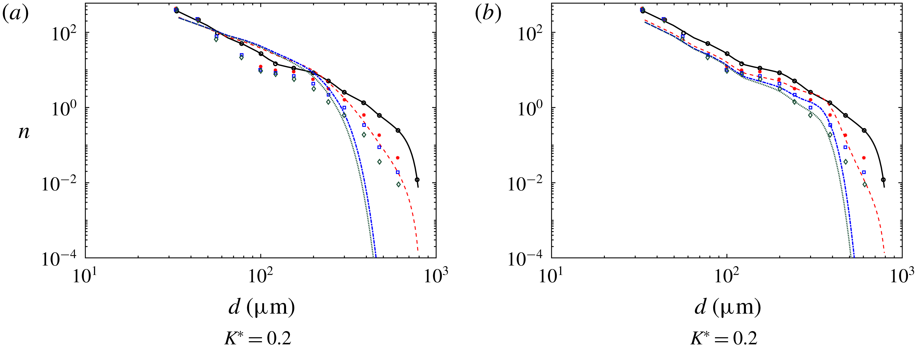
This approach results in overestimated velocities of eddies in the viscous range. In order to illustrate the net effects of this overestimation of turbulence at small scales in the overall model predictions, we can use (3.5) in (2.8) to compute the breakup frequency using
 $K^{\ast }=0.2$
for this scaling of eddy velocity (through numerical integration). We solve (3.1) and plot the resulting size distributions in figure 4. Figure 4(a) compares the computed size distributions with the experimental data. We see that there is too much breakup effect resulting in too few of the larger droplets and an increase in the concentration of the intermediate size droplets. In order to obtain a better agreement with the experiment we would need to set
 $K^{\ast }\sim O(10^{-2})$
. Thus, we conclude that in order to maintain reasonable range of value for the parameter
 $K^{\ast }$
(which is expected to be of order unity), it is important to capture both the inertial and viscous range scalings as in (2.10) for the eddy fluctuation velocity.
Time evolution of the droplet size distribution for
 $K^{\ast }=0.2$
. Panel (a) uses an inertial scaling of
 $u_{e}$
. In (b) we plot the effect of using a normal distribution proposed by Coulaloglou & Tavlarides (Reference Coulaloglou and Tavlarides1977). The symbols correspond to the experimental data,
 $t=5~\text{s}$
(○) represents the initial condition where experiment and simulation are matched,
 $t=15~\text{s}$
(*),
 $t=35~\text{s}$
(▫),
 $t=55~\text{s}$
(♢), while the lines correspond to the simulation,
 $t=15~\text{s}$
(- - -),
 $t=35~\text{s}$
(-
 $\cdot$
-
 $\cdot$
) and
 $t=55~\text{s}$
(
 $\cdots$
).

We can also study the effect of using a different breakup probability model
 $\unicode[STIX]{x1D6FD}(d_{i},d_{j})$
. We use a truncated normal distribution of Coulaloglou & Tavlarides (Reference Coulaloglou and Tavlarides1977) for simplicity. In this case it is assumed that the daughter droplet sizes for a parent drop of diameter
 $d_{j}$
are normally distributed about a mean value,
 $\bar{d}=d_{j}/2^{1/3}$
, i.e.
 $$\begin{eqnarray}\unicode[STIX]{x1D6FD}(d_{i},d_{j})=\frac{1}{s\sqrt{2\unicode[STIX]{x03C0}}}\exp \left[-\frac{(d_{i}-\bar{d})^{2}}{2s^{2}}\right],\end{eqnarray}$$
where
 $s=d_{j}/(3\times 2^{1/3})$
. This gives us a maximum probability for equal volume breakup. We plot the resulting size distributions for
 $K^{\ast }=0.2$
in figure 4(b). We observe a bump in the size distribution at
 $d\approx 300~\unicode[STIX]{x03BC}\text{m}$
and a more rapid cutoff of the large droplets as compared to figure 2(a). Additionally, we do not find an optimum value of
 $K^{\ast }$
that minimizes (3.4), i.e. the error grows with increasing
 $K^{\ast }$
. Hence, we may conclude that the form of the particular droplet breakup probability distribution is also important, though it plays a weaker role as compared to the effect of including the viscous range for this particular wave breaking case.
We demonstrate the effect of an increase in the assumed maximum eddy size allowed to break the droplets (upper limit of integration in (2.12)) in figure 5. We find that for a maximum eddy size 20 % larger than the droplet size (
 $d_{e,max}=1.2d_{i}$
), the fitted prefactor is reduced to
 $K^{\ast }=0.1$
. Using this value of
 $K^{\ast }$
we see from figure 5(a) that the steady-state size distribution is in good agreement with case where
 $d_{e,max}=d_{i}$
and
 $K^{\ast }=0.2$
. Clearly, however, the resulting breakup frequency shows some dependence on the upper cutoff of the integral (figure 5
b).
We depict the effect of changing the maximum diameter size on the size distribution and breakage frequency. In (a) the symbols correspond to the experimental data,
 $t=5~\text{s}$
(○) represents the initial condition where experiment and simulation are matched,
 $t=15~\text{s}$
(*),
 $t=35~\text{s}$
(▫),
 $t=55~\text{s}$
(♢), while the lines correspond to the simulation using
 $K^{\ast }=0.2$
,
 $t=15~\text{s}$
(- - -, red),
 $t=35~\text{s}$
(-
 $\cdot$
-
 $\cdot$
) and
 $t=55~\text{s}$
(
 $\cdots$
). The green thick dashed line (- - -, green thick) corresponds to the case where
 $d_{e,max}=1.2d_{i}$
and
 $K^{\ast }=0.1$
was used to calculate
 $g(d_{i})$
. In (b) we compare the resulting breakup frequency for the two cases,
 $d_{e,max}=1.2d_{i}$
(- - -, black) and
 $d_{e,max}=d_{i}$
(——).

3.2 Breakup of oil in a turbulent jet (Eastwood et al. Reference Eastwood, Armi and Lasheras2004)
In order to begin testing the model when applied to a system with different flow properties than the case for which
 $K^{\ast }$
was fitted, we consider the experiment by Eastwood et al. (Reference Eastwood, Armi and Lasheras2004). Oil droplets of varying density, viscosity and interfacial tension are injected continuously at the centreline in the fully developed region of a turbulent water jet. The downstream evolution of the centreline velocity and dissipation rate was well characterized and found to obey classic scalings of a turbulent round jet,
 $$\begin{eqnarray}\frac{U_{0}}{U(x)}=\frac{1}{C_{u}}\left(\frac{x}{D_{j}}-\frac{x_{0}}{D_{j}}\right),\quad \frac{\unicode[STIX]{x1D716}D_{j}}{U_{0}^{3}}=C\left(\frac{x}{D_{j}}-\frac{x_{0}}{D_{j}}\right)^{-4},\end{eqnarray}$$
where
 $C_{u}=4.08$
and
 $C=36$
are empirical constants. The virtual origin
 $x_{0}/D_{j}=5.47$
was found by fitting the experimental data with (3.7). The breakup and downstream evolution of oil droplets were tracked using digital image processing techniques (Eastwood et al.
Reference Eastwood, Armi and Lasheras2004). The authors defined a characteristic droplet size
 $d_{max}$
whose number density
 $n(d_{max})$
can only change due to its own breakup but cannot increase due to breakup of other (larger) droplets. This condition isolates the effect of the breakup frequency on the evolution of the number density. Mathematically the evolution of the size distribution can be tracked using (2.1), where for the size
 $d_{max}$
we can drop the first term in (2.2). Additionally for the quasi-one-dimensional steady-state jet flow considered, we can write the PBE for the largest size as
 $$\begin{eqnarray}\unicode[STIX]{x1D735}_{x}\boldsymbol{\cdot }[\boldsymbol{v}(d_{max},\boldsymbol{x})n(d_{max},\boldsymbol{x})]=-g(d_{max},\boldsymbol{x})n(d_{max},\boldsymbol{x}),\end{eqnarray}$$
where
 $n(d_{max},x)=N(d_{max},x)/V_{w}$
, with
 $V_{w}$
the volume of the interrogation window and
 $N(d_{\max },x)$
the total number of droplets measured in the window at
 $x$
. The droplet velocity
 $\boldsymbol{v}(d_{max},\boldsymbol{x})$
can be approximated by the local mean velocity of the turbulent jet,
 $U(x)$
. Equation (3.8) can then be written for the number of droplets
 $N(d_{max},x)$
as,
 $$\begin{eqnarray}\frac{\text{d}}{\text{d}x}[U(x)N(d_{max},x)]=-N(d_{max},x)g(d_{max},x).\end{eqnarray}$$
Dispersed fluid properties.

The maximum diameter
 $d_{max}$
represented the size where at least
 $80\,\%$
of the volume of the distribution was contained in droplets smaller than
 $d_{max}$
. The overall decay of
 $N(d_{max},x)$
with downstream distance was found to be similar when this criterion was enforced, thereby ensuring that the evolution of the largest size class is captured. In order to validate our model with the experiments, we solve (3.9) using a fourth-order explicit Runge–Kutta method (ode45 in MATLAB). Equation (2.17) is used to calculate the breakup frequency
 $g(d_{max},x)$
with
 $K^{\ast }=0.2$
for all the oils considered. A summary of the physical properties of the different oils used for the simulation along with the corresponding size
 $d_{max}$
is provided in table 1.
Evolution of
 $N(d_{max},x)$
with downstream distance for the four different oils in table 1. The symbols correspond to the experimental data of the different oils; 50 cSt silicone oil (○), olive oil (♢), 10 cSt silicone oil (▫) and heptane (*). The different lines correspond to the model; 50 cSt silicone oil (——), olive oil (-
 $\cdot$
-
 $\cdot$
), 10 cSt silicone oil (
 $\cdots$
) and heptane (- - -) with
 $K^{\ast }=0.2$
. Also shown are the model for heptane (
 ) with
 $K^{\ast }=0.1$
and 10 cSt silicone oil (
 ) with
 $K^{\ast }=0.15$
.

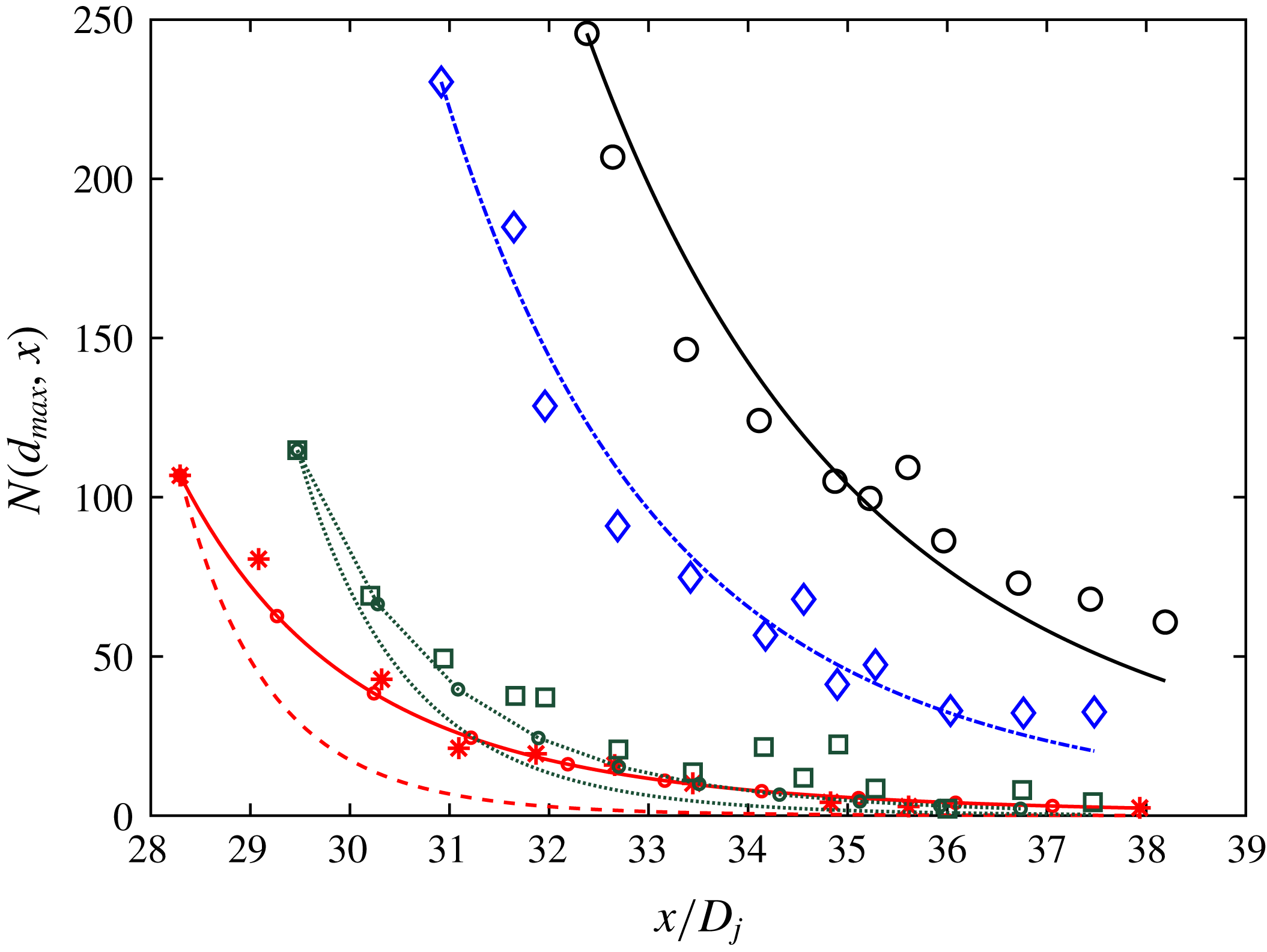
We compare the model predictions with the experimental data in figure 6. We see that the model does a good job of capturing the decay of the number of droplets for the 50 cSt silicone oil and the olive oil cases. For heptane and 10 cSt silicone oil the predicted decay is too rapid and
 $K^{\ast }=0.2$
appears not to be the optimal value, while
 $K^{\ast }=0.1$
and
 $K^{\ast }=0.15$
are seen to give better agreement with the data. We have not found any obvious parameter dependencies that could explain the different
 $K^{\ast }$
. So based on the argument that
 $K^{\ast }=0.2$
gives a good match for a majority of the applications considered, we proceed to use this value for the LES test case in the next section.
4 Application to large eddy simulation of jet in cross-flow
Large eddy simulations capture the large- and intermediate-scale turbulent motions (depending on the grid resolution), and only require modelling of the unresolved subgrid-scale turbulence effects. While the cost of LES is higher than Reynolds-averaged Navier–Stokes simulations, LES provides the ability to resolve unsteady spatially fluctuating phenomena at least down to scales of the order of the grid scale. In this work we will highlight this strength of LES in the context of simulations of the evolution and transport of size distributions of polydispersed oil droplets in water. We first describe the LES model equations, present the simulation set-up for LES modelling of a jet in cross-flow and then present results and comparisons with experimental data.
4.1 LES equations for Eulerian description of scalar transport
We adapt the code used by Yang, Meneveau & Shen (Reference Yang, Meneveau and Shen2014) and Yang et al. (Reference Yang, Chen, Chamecki and Meneveau2015) for simulations of hydrocarbon plume dispersion in ocean turbulence to simulate here a turbulent round jet with an imposed cross-flow and with oil droplets being released near the source of the jet. Let
 $\boldsymbol{x}=(x,y,z)$
with
 $x$
and
 $y$
the horizontal coordinates and
 $z$
the vertical direction, and let
 $\boldsymbol{u}=(u,v,w)$
be the corresponding velocity components. The jet and surrounding fluid are governed by the three-dimensional incompressible filtered Navier–Stokes equations with a Boussinesq approximation for buoyancy effects,
 $$\begin{eqnarray}\displaystyle & \displaystyle \unicode[STIX]{x1D735}\boldsymbol{\cdot }\tilde{\boldsymbol{u}}=0, & \displaystyle\end{eqnarray}$$
 $$\begin{eqnarray}\displaystyle & \displaystyle \frac{\unicode[STIX]{x2202}\tilde{\boldsymbol{u}}}{\unicode[STIX]{x2202}t}+\tilde{\boldsymbol{u}}\boldsymbol{\cdot }\unicode[STIX]{x1D735}\tilde{\boldsymbol{u}}=-\frac{1}{\unicode[STIX]{x1D70C}_{c}}\unicode[STIX]{x1D735}\tilde{P}-\unicode[STIX]{x1D735}\boldsymbol{\cdot }\unicode[STIX]{x1D749}^{d}+\left(1-\frac{\unicode[STIX]{x1D70C}_{d}}{\unicode[STIX]{x1D70C}_{c}}\right)\mathop{\sum }_{i}(V_{d,i}{\tilde{n}}_{i})g\boldsymbol{e}_{3}, & \displaystyle\end{eqnarray}$$
 $$\begin{eqnarray}\displaystyle & \displaystyle \frac{\unicode[STIX]{x2202}{\tilde{n}}_{i}}{\unicode[STIX]{x2202}t}+\unicode[STIX]{x1D735}\boldsymbol{\cdot }(\tilde{\boldsymbol{v}}_{i}{\tilde{n}}_{i})+\unicode[STIX]{x1D735}\boldsymbol{\cdot }\unicode[STIX]{x1D745}_{i}=\widetilde{S_{b,i}},\quad i=1,2\cdots N_{d}. & \displaystyle\end{eqnarray}$$
A tilde denotes a variable resolved on the LES grid,
 $\tilde{\boldsymbol{u}}$
is the filtered fluid velocity,
 $\unicode[STIX]{x1D70C}_{d}$
is the density of the droplet,
 $\unicode[STIX]{x1D70C}_{c}$
is the carrier fluid (sea water) density,
 $V_{d,i}=\unicode[STIX]{x03C0}d_{i}^{3}/6$
is the volume of a spherical oil droplet of size
 $d_{i}$
,
 $\unicode[STIX]{x1D749}=(\widetilde{\boldsymbol{u}\boldsymbol{u}}-\tilde{\boldsymbol{u}}\tilde{\boldsymbol{u}})$
is the subgrid-scale stress tensor with deviatoric part,
 $\unicode[STIX]{x1D749}^{d}=\unicode[STIX]{x1D749}-[tr(\unicode[STIX]{x1D749})/3]\unicode[STIX]{x1D644}$
where
 $\unicode[STIX]{x1D644}$
is the identity tensor,
 $\tilde{P}=\tilde{p}/\unicode[STIX]{x1D70C}_{r}+tr(\unicode[STIX]{x1D749})/3+|\tilde{\boldsymbol{u}}|^{2}/2$
is the pseudo-pressure, with
 $\tilde{p}$
the resolved dynamic pressure,
 ${\tilde{n}}_{i}$
is the resolved number density of the droplet of size
 $d_{i}$
and
 $\boldsymbol{e}_{3}$
is the unit vector in the vertical direction. The filtered version of the transport equation for the number density
 ${\tilde{n}}_{i}(\boldsymbol{x},t;d_{i})$
is given by (4.3). The term
 $\unicode[STIX]{x1D745}_{i}=(\widetilde{\boldsymbol{v}_{i}n_{i}}-\tilde{\boldsymbol{v}}_{i}{\tilde{n}}_{i})$
is the subgrid-scale concentration flux of oil droplets of size
 $d_{i}$
(no summation over
 $i$
implied here).
Closure for the SGS stress tensor
 $\unicode[STIX]{x1D749}^{d}$
is obtained from the Lilly–Smagorinsky eddy viscosity model (Smagorinsky Reference Smagorinsky1963),
 $\unicode[STIX]{x1D70F}_{ij}^{d}=-2\unicode[STIX]{x1D708}_{\unicode[STIX]{x1D70F}}\tilde{\unicode[STIX]{x1D61A}}_{ij}=-2(c_{s}\unicode[STIX]{x1D6E5})^{2}|\tilde{\unicode[STIX]{x1D64E}}|\tilde{\unicode[STIX]{x1D61A}}_{ij}$
, where
 $\tilde{\unicode[STIX]{x1D61A}}_{ij}=(\unicode[STIX]{x2202}\tilde{u} _{i}/\unicode[STIX]{x2202}x_{j}+\unicode[STIX]{x2202}\tilde{u} _{j}/\unicode[STIX]{x2202}x_{i})/2$
is the resolved strain rate tensor,
 $\unicode[STIX]{x1D708}_{\unicode[STIX]{x1D70F}}$
is the SGS eddy viscosity and
 $\unicode[STIX]{x1D6E5}$
is the grid (filter) scale. The Smagorinsky coefficient
 $c_{s}$
is determined dynamically during the simulation using the Lagrangian averaging scale-dependent dynamic (LASD) SGS model (Bou-Zeid, Meneveau & Parlange Reference Bou-Zeid, Meneveau and Parlange2005), which accounts for spatial inhomogeneity. The SGS scalar flux
 $\unicode[STIX]{x1D745}_{i}$
is modelled using an eddy-diffusion SGS model. We use the approach of prescribing a turbulent Schmidt and Prandtl number,
 $Pr_{\unicode[STIX]{x1D70F}}=Sc_{\unicode[STIX]{x1D70F}}=0.4$
(Yang et al.
Reference Yang, Chen, Socolofsky, Chamecki and Meneveau2016). The SGS flux can then be parameterized as
 $\unicode[STIX]{x03C0}_{n,i}=-(\unicode[STIX]{x1D708}_{\unicode[STIX]{x1D70F}}/Sc_{\unicode[STIX]{x1D70F}})\unicode[STIX]{x1D735}{\tilde{n}}_{i}$
The LES code with the LASD model has been used in a number of prior LES studies (see Porté-Agel, Meneveau & Parlange Reference Porté-Agel, Meneveau and Parlange2000; Tseng, Meneveau & Parlange Reference Tseng, Meneveau and Parlange2006; Yang et al. Reference Yang, Meneveau and Shen2014). With the evolution of oil droplet concentrations being simulated, their effects on the fluid velocity field are modelled and implemented in (4.2) as a buoyancy force term (the last term on the right-hand side of the equation) using the Boussinesq approximation. A basic assumption for treating the oil droplets as an active scalar field being dispersed by the fluid motion is that the volume and mass fractions of the oil droplets are small within a computational grid cell.
The droplet transport velocity
 $\tilde{\boldsymbol{v}}_{i}$
is calculated by an expansion in the droplet time scale
 $\unicode[STIX]{x1D70F}_{d,i}=(\unicode[STIX]{x1D70C}_{d}+\unicode[STIX]{x1D70C}_{c}/2)d_{i}^{2}/(18\unicode[STIX]{x1D707}_{f})$
(Ferry & Balachandar Reference Ferry and Balachandar2001). The expansion is valid when
 $\unicode[STIX]{x1D70F}_{d,i}$
is much smaller than the resolved fluid time scales, which requires us to have a grid Stokes number
 $St_{\unicode[STIX]{x1D6E5},i}=\unicode[STIX]{x1D70F}_{d,i}/\unicode[STIX]{x1D70F}_{\unicode[STIX]{x1D6E5}}\ll 1$
, where
 $\unicode[STIX]{x1D70F}_{\unicode[STIX]{x1D6E5}}$
is the turbulent eddy turnover time at scale
 $\unicode[STIX]{x1D6E5}$
. The transport velocity of droplets of size
 $d_{i}$
,
 $\tilde{\boldsymbol{v}}_{i}$
, is given by (Ferry & Balachandar Reference Ferry and Balachandar2001)
 $$\begin{eqnarray}\tilde{\boldsymbol{v}}_{i}=\tilde{\boldsymbol{u}}+w_{r,i}\boldsymbol{e}_{3}+(R-1)\unicode[STIX]{x1D70F}_{d,i}\left(\frac{\text{D}\tilde{\boldsymbol{u}}}{\text{D}t}+\unicode[STIX]{x1D735}\boldsymbol{\cdot }\unicode[STIX]{x1D749}\right)+O(\unicode[STIX]{x1D70F}_{d,i}^{3/2}),\end{eqnarray}$$
where
 $w_{r,i}$
is the droplet terminal (rise) velocity,
 $\boldsymbol{e}_{3}$
is the unit vector in the vertical direction and
 $R=3\unicode[STIX]{x1D70C}_{c}/(2\unicode[STIX]{x1D70C}_{d}+\unicode[STIX]{x1D70C}_{c})$
is the acceleration parameter. A more detailed discussion of the droplet rise velocity in (4.4) can be found in Yang et al. (Reference Yang, Chen, Socolofsky, Chamecki and Meneveau2016).
The term
 $\widetilde{S_{b,i}}$
in (4.3) represents the rate of change of droplet number density due to breakup and is modelled using (2.7) and (2.21) described in § 2. In implementing the model, when evaluating the filtered source term, we use the filtered parameters (e.g. grid-scale dissipation rate, etc.), that is to say, we assume
 $\widetilde{gn}\approx \tilde{g}{\tilde{n}}$
, and further that
 $\widetilde{g(\unicode[STIX]{x1D716},\ldots )}\approx g(\tilde{\unicode[STIX]{x1D716}},\ldots )$
. This means that we neglect the subgrid correlations between locally fluctuating dissipation rates at scales smaller than the grid scale and subgrid fluctuations in the concentration field. The neglect of such subgrid-scale contributions to the modelled source terms must be kept in mind, especially for applications at very high Reynolds numbers when the Kolmogorov scale is much smaller than the grid scale where further refinements and new subgrid models may be required.
The breakup rate
 $g_{i}$
is evaluated using the fits that depend on the local Reynolds number expressed in terms of the local rate of dissipation. From the SGS model, the local rate of dissipation at the LES grid scale is given by
 $$\begin{eqnarray}\unicode[STIX]{x1D716}(\boldsymbol{x},t)=2(c_{s}\unicode[STIX]{x1D6E5})^{2}|\tilde{\unicode[STIX]{x1D64E}}|\tilde{S}_{ij}\tilde{S}_{ij}.\end{eqnarray}$$
In order to capture a range of sizes the number density is discretized into
 $N_{d}=15$
bins for droplets between
 $d_{1}=20~\unicode[STIX]{x03BC}\text{m}$
up to
 $d_{N_{d}}=1~\text{mm}$
. The droplet size range is discretized according to
 $$\begin{eqnarray}d_{i+1}=2^{p}d_{i},\quad i=1,2,\ldots ,N_{d},\end{eqnarray}$$
where,
 $p=0.403$
. We then solve
 $N_{d}$
separate transport equations for the number densities
 ${\tilde{n}}_{i}(\boldsymbol{x},t;d_{i})$
with
 $i=1,2,\ldots ,N_{d}$
.
The equations (4.1) and (4.2) are discretized using a pseudo-spectral method on a collocated grid in the horizontal directions and using centred finite differencing on a staggered grid in the vertical direction (Albertson & Parlange Reference Albertson and Parlange1999). The velocity field is advanced using a fractional-step method with a second-order Adams–Bashforth scheme for the time integration. The transport equations for the droplet number densities, equation (4.3), are discretized as in Chamecki, Meneveau & Parlange (Reference Chamecki, Meneveau and Parlange2008), Yang et al. (Reference Yang, Meneveau and Shen2014) and Yang et al. (Reference Yang, Chen, Chamecki and Meneveau2015), by a finite-volume algorithm with a bounded third-order upwind scheme for the advection term (Gaskell & Lau Reference Gaskell and Lau1988). This approach prevents the appearance of negative local concentrations that tend to occur when using spectral methods. Information between the finite-volume and pseudo-spectral grids is exchanged using a conservative interpolation scheme developed by Chamecki et al. (Reference Chamecki, Meneveau and Parlange2008).
Sketch of the simulation domain and dimensions.

4.2 Simulation set-up
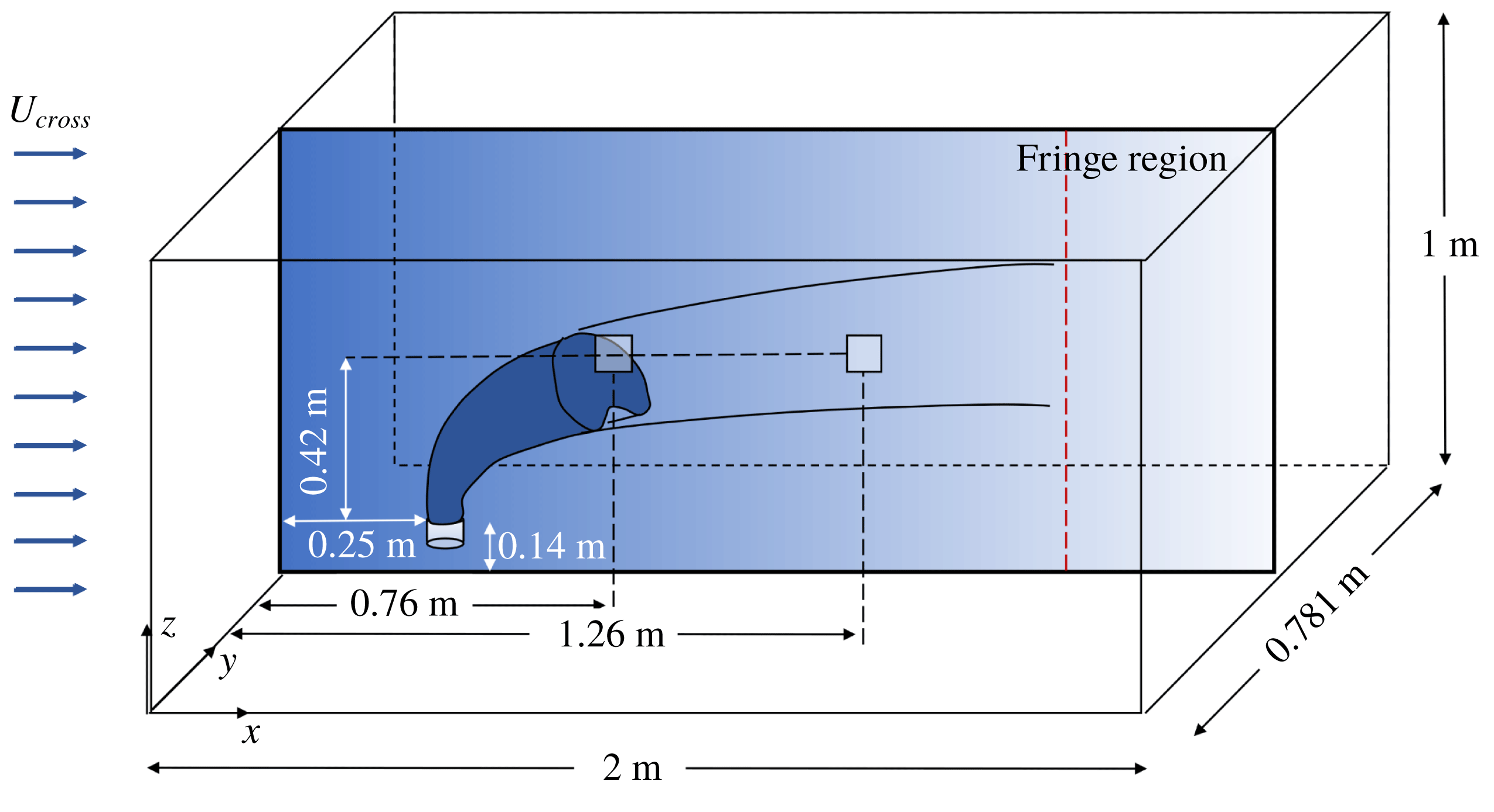
A sketch of the simulation domain is shown in figure 7. We simulate a turbulent jet with imposed cross-flow aiming to reproduce the experiments of Murphy et al. (Reference Murphy, Xue, Sampath and Katz2016), who studied a turbulent oil jet in cross-flow and measured droplet size distributions using a submersible digital inline holography technique. The experiments were carried out in a
 $2.5~\text{m}\times 0.9~\text{m}\times 0.9~\text{m}$
acrylic tank. The injection nozzle was connected to a carriage, driven by a stepper motor to generate desired cross-flow speeds. The injection nozzle had a
 $D_{expt}=4~\text{mm}$
diameter orifice and was located at a distance of
 $0.14~\text{m}$
from the bottom of the tank. The oil was injected at a flow rate of
 $Q=1.9~\text{l}~\text{min}^{-1}$
, (i.e. an injection velocity of
 $U_{j,expt}=2.5~\text{m}~\text{s}^{-1}$
) and the carriage was towed at a speed of
 $U_{c}=0.15~\text{m}~\text{s}^{-1}$
. In the experiments performed, the number of droplets was measured using a holocam fixed at the centre of the tank in the horizontal plane, and at a vertical distance of
 $0.47~\text{m}$
from the nozzle exit. It thus sampled different sections of the jet in the cross-stream direction in the course of its evolution. Numbers of droplets in various size bins were measured at two times, at
 $t=3.4~\text{s}$
and
 $t=6.9~\text{s}$
. Additionally, the total oil distribution calculated by summing over five time measurements was recorded. As the nozzle in the experiments moved with a constant speed of
 $0.15~\text{m}~\text{s}^{-1}$
, this corresponds to a downstream location of measurement at
 $x=0.76~\text{m}$
and
 $x=1.3~\text{m}$
respectively, in a frame moving with the jet nozzle (as will be done in the simulation). The total oil concentration at the measurement location height corresponds to the sum of the number of droplets measured as a function of downstream distance. In the experiments, the droplet size distributions were measured in three realizations of the experiments, hence the resulting size distribution and droplet concentrations were not fully statistically converged but the shape of the size distribution (relative size distribution) was well captured in the measurements.
As shown in figure 7, the simulations are performed in a rectangular box of size
 $(L_{x},L_{y},L_{z})=(2,0.781,1)~\text{m}$
in which the jet is stationary but a constant inflow (cross-flow) velocity is prescribed. The domain size is chosen to mimic the experimental set-up and the length is sufficiently large to capture the complete turning of the jet. The cross-flow is imposed along the
 $x$
direction while the jet is pointed in the
 $z$
direction. In order to handle the inflow and outflow conditions at the two boundaries in the
 $x$
direction within the code that uses a Fourier-series-based pseudo-spectral method, we specify a fringe zone that starts at
 $x=1.666~\text{m}$
, which damps out the velocity towards the inflow value. The simulations use a grid with
 $N_{x}\times N_{y}\times N_{z}=384\times 150\times 384$
points for spatial discretization, and a timestep
 $\unicode[STIX]{x0394}t=0.0002~\text{s}$
for time integration. The resolution in the horizontal directions is
 $\unicode[STIX]{x0394}x=\unicode[STIX]{x0394}y=5.2~\text{mm}$
, and is
 $\unicode[STIX]{x0394}z=2.6~\text{mm}$
in the vertical direction for the finite difference method. Since the latter can be regarded as requiring approximately twice as much resolution for the same accuracy, we regard the overall numerical resolution to be approximately
 $5.2~\text{mm}$
.
The injected jet is modelled in the LES using a locally applied vertically upward pointing body force, since at the LES resolution used in the simulation it is not possible to resolve the small-scale features of the injection nozzle. The applied force is spatially smoothed in a region over three grid points in
 $x,y$
and
 $z$
using a super-Gaussian smoother (of order 5 and width
 $\unicode[STIX]{x1D70E}_{G}=\unicode[STIX]{x0394}x$
) centred at
 $(x,y,z)=(0.25,0.39,0.85)~\text{m}$
.
The resulting injection velocity is controlled by the strength of the imposed body force. Since the details of the nozzle cannot be resolved, the body force is applied at a location downstream of the real nozzle, where the jet in the experiment is expected to have grown to a scale at which the numerical grid is sufficient to resolve at least the mean velocity profile. Using a classical round jet without cross-flow for calibration, the force is chosen such that the resulting centreline velocity in the LES matches the mean centreline velocity expected for the experiment at that location. More details are provided in appendix B. The location where the body force is applied is found to be
 $38.2~\text{mm}$
downstream (i.e. above) of the experimental nozzle’s virtual origin (see appendix B), while the injection velocity in the simulation is determined to be
 $U_{j,sim}=1.6~\text{m}~\text{s}^{-1}$
, i.e. lower than that in the experiment owing to the fact that the centreline velocity has already decayed at the simulated injection point. A uniform cross-flow of
 $U_{cross}=0.15~\text{m}~\text{s}^{-1}$
is imposed at the inflow boundary in order to simulate a jet in cross-flow. The droplet number density fields are initialized to zero everywhere. Oil droplets of size
 $d=1~\text{mm}$
are injected at the jet source after a delay of
 $1~\text{s}$
to allow the flow to be established. The number density transport equation for the bin corresponding to the largest droplets (
 $i=N_{d}$
with
 $d_{i}=1~\text{mm}$
) contains a source term on the right-hand side which represents injection with a specified volume flow rate that matches the experimental value of
 $Q=1.9~\text{l}~\text{min}^{-1}$
as in Murphy et al. (Reference Murphy, Xue, Sampath and Katz2016). The source is distributed over two grid points in the
 $z$
direction with weights
 $0.25$
and
 $0.75$
and over three grid points in the
 $x$
and
 $y$
directions centred at
 $x=0.245~\text{m}$
,
 $y=0.385~\text{m}$
with weights
 $0.292$
for the centre and
 $0.177$
for the neighbouring points. The physical properties of the oil and the simulation parameters are given in tables 2 and 3. The Weber number (
 $We$
) has been calculated using the near-nozzle dissipation
 $\langle \unicode[STIX]{x1D716}\rangle =30~\text{m}^{2}~\text{s}^{3}$
and the injection droplet size
 $d=1~\text{mm}$
.
Physical properties of fluids used in the simulation.

Simulation parameters.

The jet in cross-flow is simulated for a total of
 $26~\text{s}$
, corresponding to
 $13\times 10^{4}$
timesteps. The oil droplets are released after
 $t=1~\text{s}$
giving sufficient time for the jet to become fully turbulent. Starting from
 $t=12~\text{s}$
, 350 three-dimensional snapshots of the entire simulation domain are recorded for statistical analysis with an interval of
 $0.04~\text{s}$
(200 timesteps) between each snapshot.
4.3 Results
In figure 8 we show contour plots of instantaneous number density in logarithmic scale (
 $\log _{10}({\tilde{n}}_{i})$
) for four representative droplet sizes on the mid
 $y$
-plane as a function of
 $x$
and
 $z$
. The largest droplet size is in figure 8(a) and the smallest one is in figure 8(d). The spatial distributions of the number densities for different droplet sizes show distinct qualitative behaviours. The plumes of the smaller droplets appear significantly more dispersed than those of the larger sizes, showing some presence also in the bottom portions of the domain and clear effects of vertical column vortices. The largest droplets are more concentrated towards the upper portions of the overall plume (consisting of all size bins) as expected from their larger rise velocity.
Contour plots of instantaneous concentration fields at the midplane of the jet. The concentration is plotted in logarithmic scale. Panel (a) is the concentration of the droplet of size
 $1000~\unicode[STIX]{x03BC}\text{m}$
, (b) for
 $d=432~\unicode[STIX]{x03BC}\text{m}$
, (c) for
 $d=107~\unicode[STIX]{x03BC}\text{m}$
and (d) for
 $d=20~\unicode[STIX]{x03BC}\text{m}$
.

Figure 9 shows the time-averaged number density fields of the various droplet sizes at the mid
 $y$
-plane. The maximum concentration for each bin size occurs in the near-nozzle region where the energy dissipation is also the highest and thus the breakup rate is fastest. The larger droplets are more buoyant, having a larger rise velocity and thus their average plume has a higher inclination angle with respect to the cross-flow direction.
Time-averaged concentration fields at the midplane of the jet plotted in logarithmic scale. Panel (a) is the concentration of droplets of size
 $1000~\unicode[STIX]{x03BC}\text{m}$
, (b) shows the concentration field for
 $d=432~\unicode[STIX]{x03BC}\text{m}$
, (c) shows the concentration field for
 $d=107~\unicode[STIX]{x03BC}\text{m}$
and (d) shows the concentration field for
 $d=20~\unicode[STIX]{x03BC}\text{m}$
.

Contour plot of the logarithm of the averaged total volume concentration of oil showing the measurement location at
 $x=0.76~\text{m}$
and
 $x=1.3~\text{m}$
.

To make a quantitative comparison with the experiments we compare droplet size distributions measured at the two cross-stream locations indicated in figure 7. The measurement locations are centred at a vertical distance of
 $42~\text{cm}$
above the nozzle (see appendix B). The width of the bins used in the experiments is not necessarily the same as that used in the simulation. In order to make comparisons with the experiments, we define a number density normalized by the bin width, i.e.
 $$\begin{eqnarray}n_{i}^{\ast }=\frac{{\tilde{n}}_{i}}{\unicode[STIX]{x1D6FF}d_{i}},\end{eqnarray}$$
here
 ${\tilde{n}}_{i}$
is the number of droplets per
 $\text{m}^{3}$
of fluid in bin
 $i$
,
 $\unicode[STIX]{x1D6FF}d_{i}=(1/2)(d_{i+1}-d_{i-1})$
for
 $i=2$
to
 $14$
,
 $\unicode[STIX]{x1D6FF}d_{1}=d_{2}-d_{1}$
and
 $\unicode[STIX]{x1D6FF}d_{15}=d_{15}-d_{14}$
. This normalization ensures that the result is conceptually independent of the discretization of the size range, i.e. the bin width. The simulated number density fields are averaged in time and the normalized time-averaged number density
 $\overline{n}_{i}^{\ast }$
in each bin is obtained.
Since the experimental data are not fully converged statistically, a comparison of the average total oil concentration (integrated over all bins) between experiment and simulation yielded differences of factors of
 $1.4$
and
 $3.7$
at downstream locations corresponding to
 $x=0.76~\text{m}$
and
 $x=1.3~\text{m}$
respectively, in this case. Therefore, here we focus the comparison between experiment and simulation on the shape of the resulting size distribution rather than the total concentration. In particular, we normalize the size distribution for both the experiment and the simulation by the total volume concentration (
 $\bar{n}_{i}^{\ast }\times V_{i}$
) summed over the entire size range, where
 $V_{i}$
is the volume of a droplet of size
 $d_{i}$
, as defined earlier. We define the relative size distribution,
 $N_{i}^{\ast }$
according to
 $$\begin{eqnarray}N_{i}^{\ast }=\frac{\overline{n}_{i}^{\ast }}{\displaystyle \mathop{\sum }_{j}(\overline{n}_{j}^{\ast }V_{j})\unicode[STIX]{x1D6FF}d_{j}}.\end{eqnarray}$$
Figure 10 depicts the log of the total volume-averaged concentration of oil,
 $\log _{10}(\sum _{i}\overline{{\tilde{n}}}_{i}V_{i})$
. The black squares show the locations of the measurement volumes used to obtain the size distributions. We compare the relative size and volume distributions obtained from the simulations with the experimental data in figures 11–13. Panel (a) depicts the relative size distribution and (b) shows the relative volume defined by
 $N_{i}^{\ast }V_{i}$
, where
 $V_{i}$
is the volume of a particular bin. The data reported in the experiment represent an average over three realizations recorded during
 $1~\text{s}$
. In the simulation, the nozzle is fixed, and so the measurement at
 $t=3.4~\text{s}$
for the experiment translates to a window between
 $x=0.76{-}0.91~\text{m}$
. We chose a region from
 $y_{1}=0.37~\text{m}$
to
 $y_{2}=0.4~\text{m}$
and
 $z_{1}=0.56~\text{m}$
to
 $z_{2}=0.59~\text{m}$
for our measurement volume. We can see that the simulation captures the overall relative size volume distribution at this location, although the experimental data have large scatter. The number density for the smallest droplet sizes are higher in the simulation than in the experiment, and we do not observe the dip seen in the experimental data. The higher number density for the smaller sizes seen in the LES results may be due to the fact that the breakup probability function favours the formation of small droplets according to the model equation used for
 $P(d_{i},d_{j})$
. The reported data are not statistically converged and the experiment can only measure droplets with diameter larger than approximately
 $20~\unicode[STIX]{x03BC}\text{m}$
.
Comparison of LES model at
 $x=0.76~\text{m}$
for mono-dispersed injection (
 ) and bi-dispersed injection (
 ), and experimental data from (Murphy et al.
Reference Murphy, Xue, Sampath and Katz2016) measured at the corresponding time (*). (a) Relative size distribution from LES, (b) relative volume distribution.

Comparison of LES model at
 $x=1.3~\text{m}$
(
 ), and experimental data from (Murphy et al.
Reference Murphy, Xue, Sampath and Katz2016) measured at the corresponding time (*). (a) Relative size distribution from LES, (b) relative volume distribution.

Comparison of LES model averaged over a spatial window of
 $x=0.76$
–1.66 m and experimental data from (Murphy et al.
Reference Murphy, Xue, Sampath and Katz2016) (*). (a) Relative size distribution from LES, (b) relative volume distribution.

In order to explore the sensitivity of the results to the assumed initial size distribution at the injection point, we perform a second simulation in which instead of placing the entire volume injection rate into a single bin at
 $1~\text{mm}$
, it is distributed equally among the two largest bins. As shown in figure 11 (circles with dot dashed line), the results for droplets smaller than
 $400~\unicode[STIX]{x03BC}\text{m}$
are the same and are quite robust to details of the injection distribution at the large droplets.
Figure 12 shows the normalized size distribution at
 $t=6.9~\text{s}$
for the experiment corresponding to a window of
 $x=1.285{-}1.435~\text{m}$
for the simulation. We see that the relative size and volume distribution is well matched for this later time, now also including the smaller droplets. Finally, figure 13 shows the total normalized size distributions for the experiment. The total size distribution was measured in the experiment using data from 5 time instances corresponding to a spatial window
 $x=0.76{-}1.66~\text{m}$
in the simulation. We see that the model captures the relative size and volume distributions well.
We can track the plume paths of the different droplet sizes by calculating the centroid of the plume in the axial direction for each droplet size as a function of cross-stream distance. We can see from figure 14(a) that as the jet moves farther downstream, the centroid for the larger droplets moves above the smaller ones, with the difference in height being related to the difference in rise velocities as noted already. The centroid evolution for the smallest droplets shown (20 and
 $107~\unicode[STIX]{x03BC}\text{m}$
) is indistinguishable. The rise velocities for these droplet sizes are very small (
 $3\times 10^{-5}$
and
 $9\times 10^{-4}~\text{m}~\text{s}^{-1}$
, respectively) and their trajectories and plume centroids are thus dominated (equally for both droplet sizes) by mean flow and turbulence, but not appreciably by buoyancy.
(a) Evolution of centroid of various droplet plumes. (b) Logarithm of the concentration profile as function of height at a downstream distance,
 $x=1~\text{m}$
and transverse position
 $y=0.385~\text{m}$
. The lines are
 $d=1000~\unicode[STIX]{x03BC}\text{m}$
(
 ),
 $d=432~\unicode[STIX]{x03BC}\text{m}$
(-
 $\cdot$
-
 $\cdot$
),
 $d=107~\unicode[STIX]{x03BC}\text{m}$
(- - -) and
 $d=20~\unicode[STIX]{x03BC}\text{m}$
(——).

We can also examine the concentration distribution of the different sizes along the axial direction at different cross-stream locations. In figure 14(b) we plot the concentration distribution at
 $x=1~\text{m}$
. We can see that the concentration is peaked more towards the top end of the plume. This trend can be attributed to the counter-rotating vortex pair generated due to the jet in cross-flow (Cortelezzi & Karagozian Reference Cortelezzi and Karagozian2001). This results in droplets being moved from the bottom of the plume towards the top, leading to a higher concentration at the top end. We can also confirm that the plume of smaller droplets is wider than that of larger droplets, showing that the smaller droplets are more dispersed by the turbulence.
The simulation showcases the importance of including the viscous range of scales in the formulation of the breakup frequency. The Kolmogorov scale in the near-nozzle region, close to the injection location (
 $x=0.125~\text{m}$
and
 $z=0.14~\text{m}$
) where
 $\langle \unicode[STIX]{x1D716}\rangle =30~\text{m}^{2}~\text{s}^{-3}$
can be calculated as
 $\unicode[STIX]{x1D702}=(\unicode[STIX]{x1D708}^{3}/\langle \unicode[STIX]{x1D716}\rangle )^{1/4}\approx 13~\unicode[STIX]{x03BC}\text{m}$
. Droplets smaller than
 ${\approx}10\unicode[STIX]{x1D702}=130~\unicode[STIX]{x03BC}\text{m}$
would lie in the viscous range. Further downstream at the
 $y$
-mid-plane, where the average dissipation has decayed to
 $\langle \unicode[STIX]{x1D716}\rangle \approx 0.1~\text{m}^{2}~\text{s}^{-3}$
,
 $\unicode[STIX]{x1D702}\approx 60~\unicode[STIX]{x03BC}\text{m}$
. Thus most of the droplet size range is in the viscous range. Earlier models that assumed that all the sizes were in the inertial range would predict incorrect breakup frequencies for these droplets as it would overestimate the eddy fluctuation velocity at the scale of the droplet. This highlights the importance of having a framework that can smoothly transition between droplets in the inertial and viscous range.
In order to characterize the ‘typical size’ of droplets, one may evaluate the widely used Sauter mean diameter, denoted as
 $d_{32}$
, that expresses the mean diameter of the polydisperse oil by taking into account the volume to surface area ratio of the distribution. It is calculated directly from the distribution using the formula,
 $$\begin{eqnarray}d_{32}=\frac{\displaystyle \mathop{\sum }_{i}{\tilde{n}}_{i}d_{i}^{3}}{\displaystyle \mathop{\sum }_{i}{\tilde{n}}_{i}d_{i}^{2}}.\end{eqnarray}$$
Using the mean concentrations from the LES, the
 $d_{32}$
value can be computed at various locations of the flow. Figure 15 shows
 $d_{32}$
as a function of the downstream distance
 $x$
at three heights. Clearly the mean droplet size decreases as the jet flow evolves along the downstream direction of the cross-flow due to droplet breakup, although the rate of change diminishes and appears to reach a stationary scale of about
 $d_{32}\approx 300~\unicode[STIX]{x03BC}\text{m}$
at large distances away from the nozzle.
Another scale often used is the Hinze (maximum) diameter,
 $d_{max}\sim \langle \unicode[STIX]{x1D716}\rangle ^{-2/5}(\unicode[STIX]{x1D70E}/\unicode[STIX]{x1D70C}_{c})^{3/5}$
, by assuming that droplet coalescence does not occur (Kolmogorov Reference Kolmogorov1949; Hinze Reference Hinze1955) and using Kolmogorov scaling. Since here the dissipation rate varies greatly from one location to the next, it requires us to first compute the average dissipation. It is computed as the time average of
 $\unicode[STIX]{x1D716}$
according to (4.5) from the LES. Typical values are
 $\langle \unicode[STIX]{x1D716}\rangle \approx 0.6~\text{m}^{2}~\text{s}^{-3}$
at
 $x=0.3~\text{m}$
and
 $z=0.29~\text{m}$
near the nozzle, and
 $\langle \unicode[STIX]{x1D716}\rangle \approx 0.001~\text{m}^{2}~\text{s}^{-3}$
at
 $x=0.75~\text{m}$
and
 $z=0.56~\text{m}$
further downstream. Accordingly, using
 $\unicode[STIX]{x1D70C}_{c}=1018.3~\text{kg}~\text{m}^{-3}$
and
 $\unicode[STIX]{x1D70E}=1.9\times 10^{-2}~\text{N}~\text{m}^{-1}$
(see table 1), we obtain
 $d_{max}=1~\text{mm}$
near the nozzle while
 $d_{max}=18~\text{mm}$
far from the nozzle. The latter value is consistent with the fact that far from the nozzle breakup becomes far less frequent and the distribution has acquired an equilibrium value. The results show that the Hinze scale at a particular location in which the flow has large differences in dissipation rates from one location to another (as is usually the case in turbulent shear flows) cannot be used to determine the typical local droplet scale that is, instead, influenced mostly by upstream events. Note that at a few grid points from the nozzle exit, where the dissipation
 $\langle \unicode[STIX]{x1D716}\rangle \approx 30~\text{m}^{2}~\text{s}^{-3}$
the Hinze diameter,
 $d_{max}=300~\unicode[STIX]{x03BC}\text{m}$
. The dissipation in a turbulent flow is highly intermittent, a property that is captured in the current study and is discussed further subsequently. Hence, we prefer to continue the discussion of the median diameter
 $d_{32}$
and its variability in the next section.
Average
 $d_{32}$
diameter as function of downstream distance
 $x$
at various plume heights. The lines correspond to
 $z=0.55~\text{m}$
(——),
 $z=0.50~\text{m}$
(- - -) and
 $z=0.45~\text{m}$
(
 $\cdots$
).

4.4 Analysis of droplet size distribution variability in LES
As mentioned earlier, LES enables us to diagnose variability of the droplet size distributions and number density transport that RANS cannot obtain, since the latter only predicts time or ensemble average values. In order to illustrate this capability of LES, we now ask what is the inherent variability of typical droplet sizes as well as that of other practically relevant quantities.
Representative time signals (left panels) and histograms (right panels) for the Sauter mean diameter,
 $d_{32}$
at two downstream locations on the centreline. Dotted lines denote mean values.

Representative time signals (left panels) and histograms (right panels) of
 $\log _{10}(\unicode[STIX]{x1D716})$
at two downstream locations on the centreline.
 $\unicode[STIX]{x1D716}$
is in
 $\text{m}^{2}~\text{s}^{-3}$
. Dotted lines denote mean value.

We plot a time signal and histograms of the
 $d_{32}$
diameters at different plume locations in figure 16. We can see that there is a high variability of the diameter about the time-averaged mean value. This variability can be observed in LES since we are solving for three-dimensional time-dependent number density fields for each bin and so
 $d_{32}$
can be evaluated at any grid point at any timestep. At
 $x=0.75~\text{m}$
, where the averaged
 $d_{32}$
diameter is approximately
 $800~\unicode[STIX]{x03BC}\text{m}$
, we see a variability from
 $300~\unicode[STIX]{x03BC}\text{m}$
to
 $1000~\unicode[STIX]{x03BC}\text{m}$
. The probability density function (PDF) also shows non-Gaussianity, with two peaks, clearly showing that the average values of
 $d_{32}$
do not provide a complete description. The peak near
 $900~\unicode[STIX]{x03BC}\text{m}$
is affected by the discrete bins. This scale corresponds to the first bin considered in the summation corresponding to
 $d=1~\text{mm}$
.
Recall that in LES the breakup time scale depends upon the local value of dissipation, which is also known to be highly intermittent in turbulent flows. In order to illustrate the (grid-scale-averaged) dissipation intermittency, in figure 17 we show time signals of the logarithm of dissipation as well as histograms. The histogram of the logarithm of dissipation is reminiscent of Gaussian (log-normality) but with a non-Gaussian highly asymmetric tail and some outliers at very low dissipation, corresponding possibly to laminar regions outside the plume. This highly variable quantity then determines the local time scale of droplet breakup in the LES model.
Next, we consider a property that is crucial in determining reaction rates for processes that occur on the droplet surface such as bio-degradation. The total rate of bio-degradation will depend on the total surface area of the oil available for microorganisms to act upon. Given the instantaneous concentration of droplets in each bin, the instantaneous total surface area available for surface reactions can be evaluated according to
 $$\begin{eqnarray}A_{tot}(\boldsymbol{x},t)=\mathop{\sum }_{i=1}^{N_{d}}{\tilde{n}}_{i}(\boldsymbol{x},t)(\unicode[STIX]{x03C0}d_{i}^{2}).\end{eqnarray}$$
Representative signals and histograms of
 $A_{tot}(\boldsymbol{x},t)$
are shown in figure 18, again at the two locations
 $x=0.75~\text{m}$
and
 $x=0.9~\text{m}$
at
 $z=0.56~\text{m}$
and the plume centre in the transverse direction.
Representative time signals (left panels) and histograms (right panels) of total surface area of the oil per cubic metre of fluid at two downstream locations on the centreline.
 $A_{tot}$
is in
 $\text{m}^{2}~\text{m}^{-3}$
. Dotted lines denote mean values.

We can see from the panels in figure 18 that there is a high variability of the total area about the mean of approximately
 $30~\text{m}^{2}$
per cubic metre of water at
 $x=0.75~\text{m}$
and about
 $16~\text{m}^{2}$
per cubic metre of water at
 $x=0.9~\text{m}$
(even though one may expect smaller droplet sizes to be associated with an increase in total surface area, further downstream the total oil concentration has also decreased due to turbulent transport thus leading to the smaller area there). The root mean square of the surface area distribution is quite significant, of similar order of magnitude to the mean area.
It is also instructive to examine time signals and statistics of the breakup source term for each droplet size,
 $\tilde{S}_{b,i}$
, normalized by the concentration. This normalization can be interpreted as an inverse time scale for the droplet breakup, i.e. it tells us the inverse of the time taken for the number of droplets in any given bin to change appreciably over its existing value, at any given scale. In figure 19 we show representative signals of
 $\tilde{S}_{b,i}(\boldsymbol{x},t)/{\tilde{n}}_{i}(\boldsymbol{x},t)$
in logarithmic scale, as well as its histograms at two locations. As can be seen from the right panel of figure 19(a), the average values are around
 $0.5~\text{s}^{-1}$
, with very large variability about this value. It means that it takes about
 $2$
seconds for the local breakup to appreciably change the local concentration of droplets of size
 $20~\unicode[STIX]{x03BC}\text{m}$
but occasionally the breakup can be far more rapid.
Representative time signals (left panels) and histograms (right panels) of
 $\log _{10}(\tilde{S}_{b,i}/{\tilde{n}}_{i})$
for
 $d=20~\unicode[STIX]{x03BC}\text{m}$
plotted at two downstream locations of the plume at a fixed height. The values of
 $\tilde{S}_{b,i}/{\tilde{n}}_{i}$
are given in
 $1/s$
. Dotted lines denote mean values.

Finally, we document the breakup source term by plotting it in linear units for different droplet sizes, at two different locations as shown in figure 20. We can see that the time signals for the source term are highly intermittent, with the largest size (i.e. 15th bin) acting as a source for the smaller ones (negative source term in its transport equation). Further downstream at
 $x=1.56~\text{m}$
, figure 20(b) shows much smaller frequencies indicating a decreased breakup of the largest droplets. Some of the intermediate bins display both positive and negative values, as some intermediate droplet sizes act as both sources and sinks at different locations along the plume (for example see panel for
 $\tilde{S}_{b,7}/{\tilde{n}}_{7}$
in figure 20
c).
We still see a significant variance in the volume median diameter (
 $d_{32}$
) at this location despite the magnitude of the normalized source terms for the larger droplets being small. Clearly, the turbulent nature of the flow prevents us from solely relying on the averaged quantities to provide us with a complete view of the droplet size distribution in this flow, while LES contains significant amount of new information regarding the fluctuations, at least down to the grid scale.
5 Conclusions
Prediction of droplet size distributions in a turbulent flow is essential for understanding the dynamics of many types of multiphase flows. We have proposed a method to couple LES with a population balance equation to study the evolution of polydisperse oil droplets in turbulence. We use the method of classes to discretize the droplet size range into contiguous subclasses and consider the case of round droplets at relatively low volume fraction for which coalescence can be neglected. Using a jet in cross-flow as a flow application inspired by previous studies on deep-water oil spills, the model can be used to predict the turbulent transport of droplets of various sizes while accounting for breakup due to the turbulent flow field.
Time history of
 $\tilde{S}_{b,i}$
normalized by concentration for different droplet sizes at
 $z=0.56~\text{m}$
on the centreline. (a,b) represent the droplet of size
 $1000~\unicode[STIX]{x03BC}\text{m}$
at two different
 $x$
locations, (c) is the time history for
 $d=432~\unicode[STIX]{x03BC}\text{m}$
and (d) is for
 $d=20~\unicode[STIX]{x03BC}\text{m}$
. Dotted lines denote mean values.

We follow the general procedure of Konno, Aoki & Saito (Reference Konno, Aoki and Saito1982), Prince & Blanch (Reference Prince and Blanch1990) and Tsouris & Tavlarides (Reference Tsouris and Tavlarides1994) in which the breakup is modelled as due to collision of turbulent eddies with droplets. Previous models assumed the droplet size to be in the inertial range of turbulence and use Kolmogorov scaling (K41) for the velocity increment valid for the inertial range. For many applications the droplet size range can lie in the viscous subrange. We have thus proposed a model that includes the effect of the viscous range of scales of turbulence using a generalized structure function approach to characterize the eddy fluctuation velocity. The formulation contains an adjustable parameter
 $K^{\ast }$
that has been fitted using experimental data. To reduce computational cost, we parameterize the breakup frequency in terms of the various (locally changing) non-dimensional parameters, and provide practical fits that enable rapid calculation.
The population equation along with the breakup model is then implemented in an LES framework. LES enables us to accurately simulate turbulent shear flows like jets and plumes and study the advection and breakup of, for example, oil droplets in these flows. We tested the formulation by comparing the size distributions of oil droplets obtained at different locations along the plume with the experimental data of Murphy et al. (Reference Murphy, Xue, Sampath and Katz2016) and obtained good agreement for the relative droplet size distribution.
Finally, we used the LES results to quantify various new properties of the distribution as it refers to the inherent variability of turbulence. We show how the LES provides information on the variability of the median diameter, the total area available for surface reactions and illustrate the highly non-Gaussian properties of the source (reaction) terms in the transport equations for each bin of droplet concentration fields.
Clearly, additional follow-up studies are required to explore in more detail various relevant aspects such as the possible effects of the initial size distribution assumed at the nozzle exit (here we assumed a single droplet size at the injection), the effects of different breakup probability models
 $(\unicode[STIX]{x1D6FD}(d_{i},d_{j}))$
, the effects of changing grid resolution in LES, the possible effects of various subgrid-scale models for the momentum and scalar fluxes and many other possible extensions such as combining with Lagrangian models for the subgrid-scale velocity gradient fluctuations (Johnson & Meneveau Reference Johnson and Meneveau2018).
Acknowledgements
The authors thank J. Katz, D. Murphy, X. Xue, R. Ni, B. Chen and S. Socolofsky for useful conversations and insights. This research was made possible by a grant from the Gulf of Mexico Research Initiative. Computational resources were provided by the Maryland Advanced Research Computing Center (MARCC). Data are publicly available through Gulf of Mexico Research Inititative Information and Data Cooperative (GRIIDC) at https://data.gulfresearchinitiative.org (doi:10.7266/12C3ZMTD).
The fit is represented by the dashed lines whereas the numerically computed integrals are the various symbols for
 $\unicode[STIX]{x1D6E4}=10.5$
.

Appendix A. Fits for breakup frequency integral
In this section we discuss the fit for the integral in the equation for the breakup frequency derived in (2.17).
 $$\begin{eqnarray}g_{f}(Re,Oh,\unicode[STIX]{x1D6E4})=\int _{0}^{1}r_{e}^{-11/3}(r_{e}+1)^{2}\left(1+\left(\frac{r_{e}Re}{\unicode[STIX]{x1D6FE}_{2}}\right)^{-2}\right)^{-1/3}\unicode[STIX]{x1D6FA}(Oh,Re,\unicode[STIX]{x1D6E4};r_{e})\,\text{d}r_{e}.\end{eqnarray}$$
As it would be computationally intensive to evaluate an integral at every grid point for every timestep we develop an empirical form of the integral as a function of the two non-dimensional parameters
 $Re$
and
 $Oh$
, for discrete values of
 $\unicode[STIX]{x1D6E4}$
. We begin by plotting the integral
 $g_{f}$
for a wide range of Reynolds
 $Re$
and Ohnesorge
 $Oh$
numbers for a fixed value of
 $\unicode[STIX]{x1D6E4}=10.5$
. This is shown in figure 21 as the symbols for different
 $Oh$
numbers. The value of
 $\unicode[STIX]{x1D6E4}$
is chosen based on the physical properties of the oil in Murphy et al. (Reference Murphy, Xue, Sampath and Katz2016). We can see that we have a power law behaviour for higher
 $Re$
with a sharp cutoff for the small
 $Re$
. The cutoff location is a function of the Ohnesorge (
 $Oh$
) number. This suggests that we could fit
 $g_{f}$
using two power laws to capture the two extremes. The fit equation can be written as
 $$\begin{eqnarray}G(Re_{i},Oh_{i})=ax^{b}+cx^{d}-e,\end{eqnarray}$$
where
 $G=\log _{10}(g_{f})$
,
 $x=\log _{10}(Re)$
and
 $a,b,c,d,e$
are functions of
 $Oh$
. We use Matlab’s curve fitting toolbox to carry out the fitting procedure. The toolbox uses a Levenberg–Marquardt algorithm to provide the best fit for the data. We find that the coefficient
 $b$
can be fixed at
 $b=0.45$
. The other coefficients can be expressed as functions of the Ohnesorge number using the following fits as a function of
 $y=Oh$
:
 $$\begin{eqnarray}\left.\begin{array}{@{}c@{}}a(y)=a_{1}\exp (-a_{2}y)+a_{3}\exp (-a_{4}y),\\ b=0.45,\\ \displaystyle \log _{10}[-c(y)]=\frac{c_{1}y^{-c_{2}}}{1+c_{3}y^{c_{4}}},\\ \displaystyle d(y)=-\frac{d_{1}y^{-d_{2}}}{1+d_{3}y^{-d_{4}}},\\ \log _{10}[e(y)]=e_{1}\exp (-e_{2}\log _{10}(y+1))+e_{3}\exp (-e_{4}\log _{10}(y+1)).\end{array}\right\}\end{eqnarray}$$
Case
 $\unicode[STIX]{x1D6E4}=10.5$
.
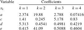
The coefficients in (A 3) for the particular value of
 $\unicode[STIX]{x1D6E4}$
chosen, are given in table 4 for
 $\unicode[STIX]{x1D6E4}=10.5$
and in table 5 for
 $\unicode[STIX]{x1D6E4}=5.45$
. The fit is valid for droplet Reynolds number less than
 $10^{4}$
and for
 $0.006\leqslant Oh\leqslant 2$
. We numerically evaluate the integral in (A 1) and compare it with the algebraic fit from (A 3) in figure 21 for four
 $Oh$
numbers. The fit is plotted using the dashed lines of different colour, while the numerically evaluated integral is represented by the symbols. We see that we have good agreement in the parameter range considered.
The fit is represented by the dashed lines whereas the numerically computed integrals are the various symbols for
 $\unicode[STIX]{x1D6E4}=5.45$
.

The fit is represented by the dashed lines computed by interpolating between
 $\unicode[STIX]{x1D6E4}_{1}=5.45$
and
 $\unicode[STIX]{x1D6E4}_{2}=10.5$
. The symbols represent the numerically computed integral for
 $\unicode[STIX]{x1D6E4}=8$
.

Case
 $\unicode[STIX]{x1D6E4}=5.45$
.
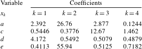
We can use the same methodology for a different value of
 $\unicode[STIX]{x1D6E4}$
. As an example, we show in figure 22 the fit for the breakup integral for
 $\unicode[STIX]{x1D6E4}=5.45$
, based on the oil properties from Johansen et al. (Reference Johansen, Brandvik and Farooq2013). We see that we can obtain a good fit for different values of
 $\unicode[STIX]{x1D6E4}$
. The coefficients for intermediate
 $\unicode[STIX]{x1D6E4}$
values can be obtained by interpolating the function
 $G(Oh_{i},Re_{i})$
between the two cases. For example, to obtain
 $g_{f}$
for
 $\unicode[STIX]{x1D6E4}=8$
we first linearly interpolate
 $G$
from
 $\unicode[STIX]{x1D6E4}_{1}=5.45$
and
 $\unicode[STIX]{x1D6E4}_{2}=10.5$
as,
 $$\begin{eqnarray}G(Re_{i},Oh_{i};\unicode[STIX]{x1D6E4})=G(Re_{i},Oh_{i};\unicode[STIX]{x1D6E4}_{1})+\frac{G(Re_{i},Oh_{i};\unicode[STIX]{x1D6E4}_{2})-G(Re_{i},Oh_{i};\unicode[STIX]{x1D6E4}_{1})}{\unicode[STIX]{x1D6E4}_{2}-\unicode[STIX]{x1D6E4}_{1}}(\unicode[STIX]{x1D6E4}-\unicode[STIX]{x1D6E4}_{1}).\end{eqnarray}$$
The integral can then be obtained as
 $g_{f}=10^{G}$
. The results from the interpolation for
 $Oh=0.042,0.09,0.35$
and
 $1$
are shown in figure 23. We see that even with a simple linear interpolation we can obtain satisfactory results.
In order to quantify the speed-up obtained by using the fits compared to the integral, we can calculate the CPU time per simulation timestep for each case. We find that the LES with the fits is 60 times faster than a LES with the breakup frequency calculated with the numerical integration of the integral at every grid point and timestep. This speed-up is more pronounced when the grid is refined. The fits are calculated using vectorized operations that are fast and efficient even on fine grids. The integral on the other hand has to be evaluated at every grid point as the integrand is a function of position.
Appendix B. Specifying the jet injection velocity in coarse LES
In this section we explain how the magnitude of the vertical jet velocity is determined so as to ensure that LES reproduces relevant quantities from the experiment. As it would be computationally expensive to resolve the small-scale structures within the nozzle in our LES, the injected jet is modelled using a locally acting body force. The jet in the experiment has a diameter of
 $d_{expt}=4~\text{mm}$
while the effective grid spacing of the LES is
 $5.2~\text{mm}$
. In order to properly resolve the turbulent inflow in the nozzle, much finer grids would be required in that region. In the LES model we take the view that we simulate a ‘coarser’ jet injection process which matches the experiments further downstream where the jet has already grown to a specified length scale and the jet centreline velocity and turbulence fluctuations have decreased. We match the length scales and centreline velocity at a particular downstream location where the jet has already grown sufficiently to match what the simulation can begin to resolve.
(a) Variation of the mean centreline velocity with axial distance in LES of jet without cross-flow using imposed body force. (b) Half-width of jet plotted as a function of axial distance. In both cases the symbols represent the simulated data, and the solid line represents the fit. The length scales in both plots are normalized with respect to the simulation diameter
 $d_{sim}=7.8~\text{mm}$
.

We calibrate the computational set-up on a jet without cross-flow and refer to well-established jet scaling laws and known correlations. First we verify that the simulated jet with an imposed smoothed vertical force reproduces well-known behaviours. We examine the centreline velocity
 $U_{0}(z)$
and the half-width of the jet (
 $r_{1/2}$
) defined as,
 $$\begin{eqnarray}\langle U(z,r_{1/2}(z),0)\rangle ={\textstyle \frac{1}{2}}U_{0}(z),\end{eqnarray}$$
where
 $z$
is the distance downstream from the nozzle exit or simulated injection point. A simulation is run using the same resolution and all other relevant parameters as in the cross-flow simulation except the cross-flow, with a vertical body force that results in a given maximum jet velocity
 $U_{j,sim}$
in the region where the force is applied. We plot the centreline velocity and the half-width from our simulation in figure 24. We can see that we recover the linear growth of the inverse centreline velocity as well as the linear scaling for the half-width. More specifically, the centreline velocity for a turbulent jet decays linearly with
 $z$
(Hussein, Capp & George Reference Hussein, Capp and George1994) and can be written as
 $$\begin{eqnarray}\frac{U_{j}}{U_{0}(z)}=\frac{(z-z_{0})}{Bd},\end{eqnarray}$$
where
 $B$
is the velocity decay coefficient and
 $U_{j}$
is the jet injection velocity. We capture the decay of the jet centreline velocity, as shown in figure 24. The slope of this line is the inverse of the product of the velocity decay constant
 $B$
times the nozzle diameter, which in the simulation is assumed to be the diameter,
 $d_{sim}$
, of an ‘effective nozzle’. Using a known value for
 $B$
, namely
 $B\approx 6$
(Hussein et al.
Reference Hussein, Capp and George1994), we can deduce
 $d_{sim}\approx 7.8~\text{mm}$
. We note that the ‘effective simulation diameter’ is almost twice the experimental jet diameter
 $d_{expt}$
.
Regarding the linear growth of the jet, the spreading rate can be determined as the slope
 $S$
,
 $$\begin{eqnarray}S=\frac{\text{d}r_{1/2}}{\text{d}z}.\end{eqnarray}$$
By fitting the figure with a straight line, we obtain
 $S=0.102$
which matches the experimental values of Hussein et al. (Reference Hussein, Capp and George1994) and Xu & Antonia (Reference Xu and Antonia2002) very well.
Next, we choose to position the body force at a location where the experimental jet is expected to have achieved the half-width equal to the simulated jet’s inflow radius, that is we require that
 $r_{1/2,expt}=d_{sim}/2$
. The applied force is spatially smoothed in a region over three grid points in
 $x,y$
and
 $z$
using a super-Gaussian smoother (of order 5 and width
 $\unicode[STIX]{x1D70E}_{G}=\unicode[STIX]{x0394}x$
) centred at
 $z_{m}$
as shown by the sketch. We recall that
 $r_{1/2,expt}(z_{m})=S(z_{m}-z_{0})$
, where
 $z_{0}$
is the virtual origin of the experimental nozzle. Using the value
 $d_{sim}=7.8~\text{mm}$
found above, we solve for
 $z_{m}-z_{0}$
and find
 $z_{m}-z_{0}=d_{sim}/(2S)=38.2~\text{mm}$
, i.e. we apply the force
 $38.2~\text{mm}$
above the location of the real nozzle’s virtual origin.
The last parameter to determine is the jet centreline velocity,
 $U_{j,sim}$
, at location
 $z=z_{m}$
. The simulated injection jet velocity will be set equal to the experimental centreline velocity at that location, thus reproducing the mean flow of the jet as the most basic condition to be met at that location, where the LES grid resolution is just sufficient to resolve a jet’s mean velocity profile. Using the classical scaling, the centreline velocity at
 $z_{m}$
in the experiment may be obtained by
 $$\begin{eqnarray}U_{0,expt}(z_{m})=\frac{U_{j,expt}Bd_{expt}}{z_{m}-z_{0}}.\end{eqnarray}$$
Setting
 $U_{j,sim}=U_{0,expt}(z_{m})$
and replacing
 $z_{m}-z_{0}=r_{1/2,expt}/\,S=d_{sim}/(2S)$
we obtain
 $$\begin{eqnarray}U_{j,sim}=\frac{2SU_{j,expt}Bd_{expt}}{d_{sim}}.\end{eqnarray}$$
Substituting
 $d_{sim}=7.8~\text{mm}$
,
 $S=0.102$
,
 $B=6$
and
 $U_{j,expt}=2.5~\text{m}~\text{s}^{-1}$
we can calculate
 $U_{j,sim}\approx 1.6~\text{m}~\text{s}^{-1}$
.
The body force magnitude is adjusted in the LES so as to achieve this value of the maximum velocity in the region where the body force is applied. With this value enforced, we obtain the desired linear growth of the jet width and the inverse linear decay of centreline velocity matching those of a classical turbulent round jet.
Sketch depicting the nozzle placement in LES (at vertical position
 $z_{m}=54~\text{mm}$
downstream of the experimental nozzle), the virtual origin of the experiment (assumed to be at
 $z_{0}=16~\text{mm}=4d_{expt}$
downstream of the nozzle), and the measurement location (at a height of
 $z_{ML}=470~\text{mm}$
above the experimental nozzle position – in the experiment with cross-flow, there is additional displacement in the horizontal direction).

To determine the corresponding location to measure the size distribution for the simulation, we note that for a classical round jet
 $z_{0}\approx 4d$
(Hussein et al.
Reference Hussein, Capp and George1994; Xu & Antonia Reference Xu and Antonia2002). We can then calculate
 $z_{m}=d_{sim}/2S+4d\approx 54.2~\text{mm}$
. The measurement volume for the experiment was located at a height of
 $47$
cm from the nozzle in the vertical direction. Therefore the measurement location for the simulation is at a vertical distance of
 $z_{ML}-z_{m}\approx 42~\text{cm}$
from the applied force position (see figure 25).