





Introduction
Glaciers are considered indicators of climate change (Oerlemans, Reference Oerlemans2005), responding rapidly to atmospheric and oceanic forcing through changes in mass balance and flow dynamics, particularly in fast-flowing systems (Meier and Post, Reference Meier and Post1987). A piedmont glacier is a unique type of glacier flowing out of a mountain range, spreading in all directions once it is free of constraining valley walls, forming a circular lobe at lower elevations (Russell, Reference Russell1893).
The formation of a piedmont lobe requires a specific combination of topographic and climatic conditions (Benn and Evans, Reference Benn and Evans2014). A favourable topographic configuration allows a glacier to flow out of a mountain range and spread into adjacent lowlands where lateral topographic constraints are weak or absent. Under such conditions, the glacier can expand laterally, forming a piedmont lobe. Additionally, a relatively high mass discharge from the accumulation zone is required to maintain a large glacier surface area below the equilibrium line. Therefore, the presence of a piedmont glacier is associated with cold-stage climatic conditions that favour glacier growth and advance to lower altitudes (Evans and Orton, Reference Evans and Orton2015). Moreover, a suitable geological substrate, i.e. soft sediments deposited at the foot of the mountains, may further promote piedmont lobe development by facilitating relatively high basal sliding and enhancing ice flow in the terminal zone (Brown and others, Reference Brown, Hallet and Booth1987).
Much more prevalent in the past, piedmont glaciers have become increasingly rare under contemporary climate conditions. Glaciers around the world are currently retreating on an unprecedented scale due to anthropogenic climate change (Zemp and others, Reference Zemp2015), and only a few piedmont glaciers in the world have survived. The remaining and most recognised examples are found in Alaska, such as the Malaspina lobe (Russell, Reference Russell1893; Muskett and others, Reference Muskett, Lingle, Sauber, Post, Tangborn and Rabus2008), and in the Canadian Arctic, for example on Axel Heiberg Island. Outside Antarctica, however, piedmont glaciers have become increasingly rare in the Southern Hemisphere. They were much more widespread in the past during the maximum extent of the Last Glacial Maximum, especially in what is presently known as the Chilean Lake District and on the eastern side of the Andes (Davies and others, Reference Davies2020). In the Chilean Lake District, located approximately 600 km north of the study area, smaller piedmont lobes formed large lakes during their retreat, including Lago Ranco, Llanquihue and Villarrica (Bentley, Reference Bentley1997).
Further south in Patagonia, the piedmont glaciers prevailed considerably longer than in other parts of the Andes (Davies and others, Reference Davies2020). A prominent example is the San Rafael Glacier, which formed a substantial piedmont lobe at the beginning of the previous century (Glasser and Jansson, Reference Glasser and Jansson2005). Subsequently, it experienced a frontal collapse, leading to the retreat of its terminus into the valley, where it undergoes a gradual inland retreat (Koppes and others, Reference Koppes, Sylwester, Rivera and Hallet2010). Such behaviour highlights the sensitivity of piedmont glaciers to environmental forcing and their susceptibility to rapid recession.
For calving glaciers, the transition from grounded to floating ice is a key process influencing frontal stability and subsequent retreat (Walter and others, Reference Walter, O’Neel, McNamara, Pfeffer, Bassis and Fricker2010). Once a glacier detaches from the bed and becomes afloat, the balance of forces and stresses changes substantially, affecting flow dynamics and calving (Tsutaki and others, Reference Tsutaki2019; Pronk and others, Reference Pronk, Bolch, King, Wouters and Benn2021). Despite its importance, there is considerable uncertainty regarding the time elapsed between the onset of buoyancy and the eventual fragmentation and disintegration of floating ice (Sutherland and others, Reference Sutherland, Carrivick, Gandy, Shulmeister, Quincey and Cornford2020). The process of calving itself has been investigated for glaciers terminating in lakes (Boyce and others, Reference Boyce, Motyka and Truffer2007), particularly in Patagonia (Warren and others, Reference Warren, Benn, Winchester and Harrison2001) and New Zealand (Warren and Kirkbride, Reference Warren and Kirkbride2003). However, these studies do not provide an exact timing for when glaciers reached flotation. Moreover, direct observations of the collapse of a piedmont glacier are rare, with most existing work based on reconstructions of past changes in glacier area, such as those inferred for former piedmont lobes in the Chilean Lake District (e.g. Lago Ranco; Bentley, Reference Bentley1997).
In this context, the position of the grounding line—the boundary between grounded ice and the detached, floating part—is typically determined with indirect methods, mostly employing Synthetic Aperture Radar (SAR) interferometry or flow modelling. The relatively few direct studies generally combine these approaches with ground-penetrating radar (GPR) surveys (Antropova and others, Reference Antropova, Mueller, Samsonov, Komarov, Bonneau and Crawford2024) and have focused primarily on Antarctic shelf glaciers and Greenland outlet glaciers (MacGregor and others, Reference MacGregor, Anandakrishnan, Catania and Winebrenner2011; Rosenau and others, Reference Rosenau, Schwalbe, Maas, Baessler and Dietrich2013; Mayer and others, Reference Mayer2018). GPR measurements allow ice thickness to be constrained and additionally provide information on basal conditions, including the presence of water beneath the glacier, inferred from the strength of the reflected radar signal (Copland and Sharp, Reference Copland and Sharp2001).
To address recent changes observed at the front of San Quintín Glacier, a helicopter-borne GPR survey was conducted in May 2019 in the terminal zone of the glacier to directly constrain ice thickness, bed conditions and the presence of water at the glacier bed. These measurements, analysed together with satellite-derived ice velocity, frontal position and surface elevation change, allow us to assess grounding line position and the role of basal water and buoyancy in controlling glacier flow and calving dynamics.
Study area
This study focuses on San Quintín Glacier, the last piedmont glacier in the Andes (Davies and others, Reference Davies2020), located in southern Chile (Fig. 1). Originating from the Northern Patagonia Icefield (NPI) plateau, it flows westward towards the Istmo de Ofqui, where it forms a large piedmont lobe. The NPI is the second-largest ice mass in South America with a surface area of about 4000 km $^2$ (Aniya, Reference Aniya1988; Rivera and others, Reference Rivera, Benham, Casassa, Bamber and Dowdeswell2007; Windnagel and others, Reference Windnagel2023). While many outlet glaciers of the NPI experience frontal retreat (Willis and others, Reference Willis, Melkonian, Pritchard and Ramage2012), there are notable exceptions of relatively stable front positions in recent decades, most prominently San Rafael Glacier, which decelerated its retreat after undergoing frontal collapse of its lobe (Mouginot and Rignot, Reference Mouginot and Rignot2015; Collao-Barrios and others, Reference Collao-Barrios2018). Overall, the NPI experiences a net negative surface mass balance of -0.6
 $\pm$2.1 m w.e. a−1 (Bravo and others, Reference Bravo, Bozkurt, Ross and Quincey2021), leading to a sustained lowering of the ice surface since the late 1970s (Willis and others, Reference Willis, Melkonian, Pritchard and Ramage2012; Abdel Jaber and others, Reference Abdel Jaber, Rott, Floricioiu, Wuite and Miranda2019; Dussaillant and others, Reference Dussaillant2019), with thinning rates reaching -1.00
 $\pm$0.01 m a
 $^{-1}$ between 2000 and 2014 (Braun and others, Reference Braun2019). Accordingly, the NPI contributes to observed sea-level rise with an estimated cumulative sea-level equivalent of 0.20
 $\pm$0.03 mm between 1975 and 2000 (Rignot, Reference Rignot2003).
Map of the study area and the Northern Patagonia Icefield, (upper inset): general location, (lower inset): San Quintín Glacier with marked GPR profiles in the terminal part. Background image: Sentinel-2A acquired on 16/04/2017. UTM 18S (WGS84) coordinates are used here and in all subsequent map-based figures.

Figure 1 Long description
Map of the Northern Patagonia Icefield in southern Chile, highlighting glaciers such as San Quintín, San Rafael and Steffen. The map includes geographic coordinates and a scale bar indicating distances in kilometers. An inset at the top left shows the general location within South America. Another inset at the bottom left provides a detailed view of the San Quintín Glacier with marked GPR profiles. The map uses UTM 18S (WGS84) coordinates and features labels for key glaciers and the icefield. The background image is from Sentinel-2A, acquired on April 16, 2017.
San Quintín Glacier is currently the largest outlet glacier of NPI (763.3 km $^2$ in 2019; DGA, 2022). It calves into an unnamed freshwater lagoon closed by a terminal moraine system (Glasser and others, Reference Glasser, Jansson, Harrison and Rivera2005). Due to the restricted river outflow from the lagoon, the discharge of icebergs to the ocean is limited (Podgórski and Petlicki, Reference Podgórski and Petlicki2020). The glacier flows to the western side of the NPI, making it susceptible to the highly humid and temperate maritime climate prevalent in the region (Lenaerts and others, Reference Lenaerts2014). As a result, rapid thinning has been observed (Braun and others, Reference Braun2019), driven by a strongly negative mass balance, with ablation rates locally surpassing 10 m a−1 (Schaefer and others, Reference Schaefer, Machguth, Falvey and Casassa2013) and further enhanced by dynamic stretching.
Historical observations indicate that San Quintin Glacier extent was substantially larger in the early twentieth century. During his expedition to Patagonia in an effort to map the continental divide, Hans Steffen (Reference Steffen1900) described this glacier as notably larger compared to the adjacent San Rafael Glacier. Subsequent mapping by the Swedish expedition led by Otto Nordenskiöld in 1920–21 (Pallin, Reference Pallin1933) indicates that the piedmont lobe extended 700-3500 m beyond the present lagoon boundary, most prominently to the north and south, while the extension along the main flowline was more limited. Since then, San Quintín Glacier has received limited attention in terms of comprehensive studies, primarily due to its challenging accessibility and logistical constraints. Existing work has focused primarily on its terminal moraines (Winchester and Harrison, Reference Winchester and Harrison1996; Harrison and others, Reference Harrison, Warren, Winchester and Aniya2001), or has relied predominantly on remote sensing observations (Podgórski and Petlicki, Reference Podgórski and Petlicki2020).
Consequently, large-scale studies of the ice elevation change (Rignot, Reference Rignot2003; Rivera and others, Reference Rivera, Benham, Casassa, Bamber and Dowdeswell2007; Abdel Jaber and others, Reference Abdel Jaber, Rott, Floricioiu, Wuite and Miranda2019; Braun and others, Reference Braun2019), ice thickness (Gourlet and others, Reference Gourlet, Rignot, Rivera and Casassa2016; Millan and others, Reference Millan2019; Fürst and others, Reference Fürst2024) or glacier mass balance (Schaefer and others, Reference Schaefer, Machguth, Falvey and Casassa2013; Bravo and others, Reference Bravo, Bozkurt, Ross and Quincey2021; Minowa and others, Reference Minowa, Schaefer, Sugiyama, Sakakibara and Skvarca2021) of NPI remain weakly constrained with in situ measurements on one of its largest outlet glaciers. More generally, this scarcity of direct observations highlights the need for additional ground-truth data for key glaciological and climatological variables in Patagonia (Ruiz and others, Reference Ruiz, Pitte, Rivera, Schaefer, Masiokas, Mataloni and Quintana2022). Specifically, comprehensive measurements of ice thickness in the frontal parts of the Patagonian outlet glaciers are still lacking (Millan and others, Reference Millan2019; Fürst and others, Reference Fürst2024). This limitation, together with inconsistencies among the outcomes of inverse modelling estimates (Carrivick and others, Reference Carrivick, Davies, James, Quincey and Glasser2016; Farinotti and others, Reference Farinotti2019), hampers accurate calculations of mass flux and partitioning between frontal ablation and surface mass balance, both of which depend critically on accurate front geometry (Bown and others, Reference Bown, Rivera, Petlicki, Bravo, Oberreuter and Moffat2019; Minowa and others, Reference Minowa, Schaefer, Sugiyama, Sakakibara and Skvarca2021).
Data and methods
Airborne GPR
In May 2019, a field campaign was conducted on the terminal part of San Quintín Glacier using a helicopter-borne GPR. We used an in-house GPR system that included a high-voltage impulse transmitter (3.2 kV peak output, with a rise time pulse of 8 ns), a signal acquisition receiver, a laser altimeter and a dual-frequency GPS (Zamora and others, Reference Zamora, Uribe, Oberreuter and Rivera2017). The system utilised a dual broadband bow-tie antenna operating at a central frequency of 20 MHz. The antenna was contained within a metal structure of 8.0 $\times$4.8
 $\times$1.2 m (
 $\sim$350 kg) hanging 20 m below the helicopter during measurement. The received signal was digitised by a 14-bit analogue-to-digital converter at a sampling frequency of 400 MHz, which determines the system’s vertical resolution of approximately 5 m (Mingo and others, Reference Mingo, Flowers, Crawford, Mueller and Bigelow2020). During the survey, the GPR was set to pulse repetition frequency of 3 kHz with a stacking of 256 traces. With this configuration and a flight speed of 20 m s
 $^{-1}$, a radar trace was obtained at approximately 2 m intervals. This system is capable of penetrating up to 700 m of temperate ice in Patagonia (Millan and others, Reference Millan2019).
The radar data were geo-located using differential GPS, using the GPR GPS receiver and a GPS base station located in Puerto Guadal, approximately 80 km east of the study site. Two-way travel times and amplitudes of the radar reflectors were determined using Reflexw software (http://www.sandmeier-geo.de/), and the ice thickness was calculated assuming constant velocity of electromagnetic wave propagation in ice of 0.168 m ns $^{-1}$ (Glen and Paren, Reference Glen and Paren1975), a value commonly used for Patagonian glaciers (Blindow and others, Reference Blindow, Salat and Casassa2012; Gacitúa and others, Reference Gacitúa, Uribe, Wilson, Loriaux, Hernández and Rivera2015). This value is typically estimated using the hyperbolae method, which infers wave velocity from the curvature of diffraction hyperbolae produced by point reflectors. In our case, significant noise in radargrams of temperate ice prevented a reliable application of this method, and a constant velocity was therefore assumed. The surface and bottom reflectors were manually selected in Reflexw. Several data processing steps were applied to the raw data, including static correction (to account for variable antenna height), band-pass filtering (to suppress noise outside the antenna bandwidth), background removal (to reduce coherent noise), equidistant trace interpolation (to ensure uniform along-track sampling), 2D diffraction migration (to improve reflector positioning) and a gain function (to compensate for signal attenuation with depth).
The elevation of the glacier surface was estimated by subtracting the radar distance between the antenna and the surface from the GPS elevation of the antenna, assuming an airwave speed of 0.3 m ns $^{-1}$. The main source of error in estimating ice thickness stemmed from the assumption of electromagnetic wave velocity, which depends on snow and ice density and water content. Taking into account additional sources of uncertainty, such as GPS positioning, radar resolution and picking, following the approach of Lapazaran and others (Reference Lapazaran, Otero, Martín-Español and Navarro2016), the estimated uncertainty in ice thickness was approximately 6%. Ice thickness differences compared at crossing points of intersecting GPR profiles were found to fall within this limit.
Bedrock reflection power
The depth to the bedrock and the presence of water at the glacier bed were determined by analysing the strength of the reflection signal. To quantify the properties of the reflection from the glacier bed, we utilised the Bedrock Reflection Power (BRP). The BRP was calculated based on a radar profile and the vectorisation of the air-ice and ice-bed interfaces, following the methodology of Gades and others (Reference Gades, Raymond, Conway and Jacobel2000):
 \begin{equation}
BRP=\frac{1}{n_2-n_1+1}\sum_{n=n_1}^{n_2} S_n^2
\end{equation}
where  $S_n$ is the amplitude of the radar signal in each sample;
 $n_1$ and
 $n_2$ are the initial and final sample numbers of the time window that includes the background reflector. The values
 $n_1$ and
 $n_2$ were chosen following Copland and Sharp (Reference Copland and Sharp2001).
The Internal Reflection Power (IRP) is a measure of the radar signal power averaged over the entire ice column, calculated between the air-ice interface ( $n_0$) and the ice-bed interface (
 $n_1$):
 \begin{equation}
IRP=\sum_{n=n_0}^{n_1} S_n^2
\end{equation}
In this case, the Copland and Sharp (Reference Copland and Sharp2001) guidelines were again followed for the choice of  $n_0$ and
 $n_1$. In contrast to Eq. (1), where the summation window is restricted to the bed reflection and normalised by the analysed layer thickness, Eq. (2) integrates the signal over the full ice depth range and is used as an indicator of overall internal scattering.
The traces with ice thickness greater than 600 m were filtered and removed from the BRP analysis, as they fall outside the linear thickness range used for the attenuation estimation and do not allow for a reliable assessment of Bed Reflection Power. The estimate of BRP from Equation 1 depends on the attenuation by geometric divergence and the dielectric properties of the ice. Therefore, an estimated BRP ( $BRP_e$) is calculated to compensate for these effects and finally obtain a
 $BRP_r$ (Residual Bed Reflection Power), which is a measure of bed properties. In areas of high IRP, strong scattering and attenuation may limit radar penetration to the glacier bed, such that lower BRPr values may reflect signal loss within the ice column rather than properties of the bed itself (Gades and others, Reference Gades, Raymond, Conway and Jacobel2000).
 $BRP_r$ is defined as:
 \begin{equation}
BRP_r=\frac{BRP}{BRP_e}
\end{equation}
To determine  $BRP_e$, we start with the radar equation:
 \begin{equation}
P_{rx}=P_{tx} G L_g T_{12}^2 L_i^2 R_{23}
\end{equation}
where  $P_{rx}$ is the power received,
 $P_{tx}$ is the transmitted power (76.12 dBm),
 $G$ is the total combination of gains and losses of the radar system (5.3 dB),
 $L_g$ is the geometric divergence loss,
 $T_{12}$ is the transmission loss at the air-ice interface,
 $L_i$ is the dielectric loss in the ice column and
 $R_{23}$ is the background reflection coefficient. Thus, we can write
 \begin{equation}
BRP_e=P_{tx} G L_g T_{12}^2 L_i^2
\end{equation}
The loss due to geometric divergence in the case of aerial measurements (Gacitúa and others, Reference Gacitúa, Uribe, Wilson, Loriaux, Hernández and Rivera2015) is given by the following:
 \begin{equation}
L_g = \frac{\left(G\lambda \right)^2}{\left[8\pi \left(h_a+\frac{H}{\sqrt{\varepsilon_i}}\right) \right]^2}
\end{equation}
where  $\lambda$ is the wavelength in the air,
 $\varepsilon_i$ is the relative dielectric permittivity of the ice,
 $H$ is the thickness of the ice and
 $h_a$ is the thickness of the air layer. The dielectric loss in ice is obtained with the expression (Jacobel and others, Reference Jacobel, Welch, Osterhouse, Pettersson and MacGregor2009):
 \begin{equation}
L_i=e^{-2H/L_a}
\end{equation}
where  $L_a$ is the average length of attenuation, which is related to the average attenuation rate
 $N_a$ (in dB km−1) through the following relationship:
 \begin{equation}
N_a=10^3\left(10\log_{10}e\right)L_a^{-1}
\end{equation}
This expression was obtained by linearising the equation 4 after normalising it with the term  $L_g$. Consequently, the attenuation of the ice, denoted as
 $N_a$ (in dB km−1), was calculated using the empirical method proposed by Jacobel and others (Reference Jacobel, Welch, Osterhouse, Pettersson and MacGregor2009). The calculation was based on a linear regression analysis that considered the decay of the amplitude with the depth of the ice, within the linear range of the dispersion from 200 to 600 m in ice thickness. The results of the attenuation, specifically the depth-averaged attenuation, are depicted in Figure 2. According to a compilation of various studies by Hills and others (Reference Hills, Christianson and Holschuh2020),
 $N_a$ typically ranges from 5 to 30 dB km−1 in cold ice. However, the obtained values are slightly higher, which can be attributed to the temperate structure of the ice, characterised by an increased attenuation resulting from the higher liquid water content.
Scatter plot of the normalised Bedrock Reflection Power (BRP) vs. ice thickness along the transverse profiles BB’ and CC’ (see location in Fig. 1). The grey shaded area corresponds to ice thickness lower than 200m where the linear relationship does not hold.

Figure 2 Long description
The horizontal axis label reads Ice thickness H (m). The horizontal axis shows values from 0 to 600. The vertical axis label reads Normalised BRP (dB). The vertical axis shows values from 80 to 140. Two groups of circular points are shown, with one group matching the legend entry BB′ and the other group matching the legend entry CC′. A shaded vertical band spans from 0 to 200 on the horizontal axis. A diagonal fitted line slopes downward from left to right across the point cloud. Text along the line reads Na equals 32.7 dB km superscript minus 1. The point cloud is densest from about 100 to 550 on the horizontal axis and from about 105 to 135 on the vertical axis. Points extend to about 600 on the horizontal axis and to about 140 on the vertical axis. The legend text reads: BB′ Na equals 35.5 plus or minus 1.4 dB km superscript minus 1, R superscript 2 equals 0.63. CC′ Na equals 29.9 plus or minus 0.7 dB km superscript minus 1, R superscript 2 equals 0.77.
The measured Bedrock Reflection Power follows a linear relationship with the ice thickness across all the recorded profiles (Fig. 2). This relationship allows for the elimination of geometric factors, enabling the calculation of BRPr that is solely related to the properties of the glacier bed. With the estimated  $N_a$ of 32.7 dB km−1,
 $BRP_e$ and
 $BRP_r$ were calculated. The gain
 $G$ parameter in Equation 6 was adjusted individually for each profile to ensure that the mean
 $BRP$ is not lower than the mean
 $BRP_e$. The resulting values were
 $G_{AA'}$ = 97.53,
 $G_{BB'}$ = 97.83 and
 $G_{CC'}$ = 100.7.
Remote sensing of glacier geometry and ice flow
We calculate the ice extent’s elevation change using satellite Digital Elevation Models (DEMs) derived from VHR satellite imagery, specifically Worldview-2 (2017) and Pléiades (2019), in combination with the Shuttle Radar Topography Mission (SRTM) DEM from 2000 and the TanDEM-X DEM from 2011 to 2015. The VHR images were processed using ERDAS IMAGINE software to generate DEMs with a resolution of 2 m and estimated accuracy of 1.70 m. Further information on the generation of these DEMs can be found in the Appendix, Sect. A1A.
The glacier extent was manually mapped using the GEEDiT (Google Earth Engine Digitisation Tool), an interactive environment for visual interpretation and digitisation of glacier boundaries from satellite imagery (Lea, Reference Lea2018). Glacier outlines were delineated on a collection of optical imagery, including Landsat 4-5, 7, 8 and Sentinel-2, spanning the period from 1986 to 2020. Frontal positions were delineated visually based on the contrast between ice, open water and ice mélange, using the highest quality imagery available for each epoch, and applying a consistent interpretation criterion along the entire calving front. The outlines therefore represent interpreter-based mapping following standard practice in glacier remote sensing studies. Previous studies based on repeated independent digitisation of glacier termini indicate that manual delineation typically results in deviations on the order of several tens of metres, reflecting the point-by-point visual interpretation inherent to this approach (Brough and others, Reference Brough, Carr, Ross and Lea2019; Fahrner and others, Reference Fahrner, Lea, Brough, Mair and Abermann2021; Lu and others, Reference Lu, Jiang, Li, Liu, Sole and Livingstone2026). Given the magnitude of the observed changes in this study (hundreds of metres to kilometres), this level of uncertainty does not affect the conclusions of the present analysis. A separate quantitative assessment of delineation uncertainty was therefore not introduced, as it would lack an independent dataset for validation.
The lobe length, area and Minkowski fractal dimension  $D$ were all derived from the manually digitised frontal outlines using QGIS. Lobe length and area were calculated directly from the outlines, while the Minkowski fractal dimension
 $D$ was obtained using a box-counting approach following Edgar (Reference Edgar and Edgar2008), providing a relative measure of calving front shape complexity.
Ice flow velocities were extracted from two publicly available global datasets. The FAU RETREAT database provides monthly velocity mosaics for the period 2015–21 derived from Sentinel-1 SAR intensity cross-correlation, with a spatial resolution of approximately 200 m (Friedl and others, Reference Friedl, Seehaus and Braun2021). In addition, ice flow velocities were obtained from the NASA MEaSUREs ITS_LIVE project, which provides yearly velocity mosaics derived from optical Landsat imagery processed using the auto-RIFT algorithm, at a spatial resolution of 120–240 m (Gardner and others, Reference Gardner2018; Reference Gardner, Fahnestock and Scambos2019), covering the period 1986–2018. Together, these datasets encompass the entire study period from 1986 to 2021, with the exception of data gaps between 1987 and 1998.
Ice buoyancy
For grounded glaciers, ice surface elevation change  $\Delta{Z}$ is equivalent to ice thickness change
 $\Delta{H}$. Nonetheless, in scenarios where the ice is unsupported at the base and instead floating, it becomes important to account for the elevation fluctuations of the glacier bed. This factor significantly offsets a substantial portion of the ice thickness variation resulting from buoyancy effects. As a result, the ice elevation change for an ice shelf or floating tongue is generally one order of magnitude smaller compared to a grounded tidewater glacier experiencing an equivalent change in ice thickness. First, let us introduce the flotation criterion, denoted as
 $f$, which depends on the density of both the submerged material and the surrounding fluid:
 \begin{equation}
f=\frac{\rho_i}{\rho_w}
\end{equation}
Following measurements conducted by Schwikowski and others (Reference Schwikowski, Schläppi, Santibañez, Rivera and Casassa2013) at the Pío XI glacier, we adopted an ice density  $\rho_i$ of 900 kg m
 $^{-3}$. Considering the density of fresh water
 $\rho_w$ as 1000 kg m
 $^{-3}$, we set the value of
 $f$ to 0.90. The relative water height
 $\omega$ is a measure of a portion of the cliff that is below the water level:
 \begin{equation}
\omega=\frac{h_w}{H}=1-\frac{h}{H}
\end{equation}
where  $h_w$ is the thickness of the ice below the water level,
 $H=h+h_w$ is the total thickness of the ice and
 $h$ is the thickness of the ice above the water level. When
 $\omega$ approaches
 $f$ (0.90), the ice reaches flotation. For lower
 $\omega$ values, it is useful to consider the height above flotation
 $h_f$ as a measure of the stability of grounding:
 \begin{equation}
h_f=H-\frac{h_w}{f}
\end{equation}
This value provides information about the extent to which the ice supports the ice column before it becomes buoyant. Studies on tidewater glaciers have established a connection between the parameters  $\omega$ and
 $h_w$ with calving intensity (Mercenier and others, Reference Mercenier, Lüthi and Vieli2018; Bown and others, Reference Bown, Rivera, Petlicki, Bravo, Oberreuter and Moffat2019). In the case of lacustrine calving, the ice front typically becomes unstable upon reaching flotation, resulting in the disintegration of the ice into large tabular icebergs subsequent to full-thickness calving (Warren and others, Reference Warren, Benn, Winchester and Harrison2001; Carrivick and others, Reference Carrivick, Tweed, Sutherland and Mallalieu2020). By knowing the distance above flotation and assuming a constant rate of ice thinning (
 $\dot{H}$), it is possible to calculate the time required to reach flotation (
 $t_r$):
 \begin{equation}
t_r=\frac{h_f}{\dot{H}}
\end{equation}
The grounding line position was derived by combining several independent indicators. Where available, direct information from GPR profiles was used to identify the transition from grounded to floating ice based on bed geometry and ice thickness. Away from the GPR profiles, the grounding line was inferred from patterns of surface elevation change and relative water height, using the flotation criterion described above. In particular, areas exhibiting high BRP $_r$, low surface elevation change rates and relative water heights approaching flotation were interpreted as floating, whereas upstream regions showing stronger surface lowering were considered grounded. This approach provides a physically consistent, observation-based estimate of grounding line position without relying on flow modelling.
Results
Ice thickness and bed properties
The radio echo sounding results show an ice thickness of 215 m at the glacier front, with only a minor increase of 25 m over the first 1.4 km up-glacier along the longitudinal profile AA’. Further upstream, ice thickness increases substantially, reaching values up to 600 m approximately 6 km from the 2019 terminus position (Fig. 3a and b). Across the transverse profiles BB’ (Fig. 3b) and CC’ (Fig. 3d), ice thickness generally increases from the valley walls towards the intersections with the longitudinal profile AA’. Both profiles show a weak asymmetry in the across-flow thickness distribution. Profile BB’ connects exposed bedrock at the valley gateway to the proglacial lake, and records a strong thickness gradient across the terminal part of the lobe. Along profile CC’, the minimum ice thickness is reached slightly north of its intersection with profile AA’. At the intersection points between the transverse and the longitudinal profiles, ice thickness values are consistent within the measurement uncertainty. Along profile AA’, a local thickness minimum is observed immediately upstream of its intersection with profile BB’.
Ground-penetrating radar profiles of San Quintín Glacier measured on 19 May 2019: (a) Ice thickness profiles, (b–d) radargrams with manually delineated glacier bed (purple) and air-ice interface (blue) (upper panels), and residual bed reflection power BRP $_r$ (red) and internal reflection power IRP (black) along the longitudinal profile AA’ (b), and transverse profiles BB’ (c) and CC’ (d) (lower panels). Solid lines indicate moving average values of BRP
 $_r$ (red) and IRP (black), shown to highlight large-scale spatial variability along each profile. Background image: Pléiades, 24 April 2019 (Pléiades © CNES 2019, distribution Airbus D&S).

Figure 3 Long description
Ground penetrating radar profiles of San Quintín Glacier measured on 19 May 2019 are shown in four panels. Panel (a) displays an aerial view with marked profiles AA’, BB’ and CC’. Panel (b) shows a radargram along the longitudinal profile AA’. The vertical axis is labeled ′Elevation (m)′ ranging from 0 to 2500 meters, representing subsurface reflectivity amplitude. The horizontal axis is labeled ′Distance along profile (km)′ ranging from 0 to 10 kilometers. The glacier bed is delineated in purple and the air-ice interface is in blue. Below the radargram, residual bed reflection power (BRP) in red and internal reflection power (IRP) in black are plotted, with the vertical axis labeled ′BRP (dB)′ ranging from -60 to 0 decibels. BRP indicates bed reflection strength, while IRP measures internal scattering. Higher BRP values suggest stronger bed reflections and higher IRP values indicate more internal scattering. Panel (c) shows the transverse profile BB’, with similar labeling and plotting of BRP and IRP. Panel (d) displays the transverse profile CC’, again with similar labeling and plotting. Solid lines indicate moving average values of BRP and IRP, highlighting spatial variability along each profile. Notable observations include an increase in ice thickness along AA’, with a local minimum upstream of BB’. BRP and IRP show variability, with peaks and troughs indicating changes in reflection power along the profiles.
The glacier bed has a reverse slope along the longitudinal profile AA’, with a minimum bed elevation of approximately 400 m below sea level (Fig. 3a). Along the transverse profiles BB’ and CC’, located within the confined valley, the bed geometry follows a parabolic and slightly skewed shape (Fig. 3b and c). The ice body shows high radar scattering and no clearly visible internal structures.
Along the longitudinal GPR profile AA’, BRPr shows pronounced spatial variability, with the highest values observed near the glacier front (Fig. 3). Isolated regions of elevated BRPr are also present within glacier bed overdeepings near km 2.5 and 4.3 along profile AA’. In contrast, IRP values are generally spatially uniform, with isolated higher values corresponding to highly crevassed areas or local water inclusions. The highest IRP values are found near 2.4 and 3.2 km along profile AA’. Both BRPr and IRP show high local variability, as indicated by the scatter of individual measurements, while the large-scale spatial trends highlighted by the moving average profile remain well defined.
Ice extent and recent elevation change
The San Quintín Glacier front experienced a retreat of over 3 km between 1993 and 2020, coincident with the formation of a large lagoon surrounding the remains of its piedmont lobe (Fig. 4a). The retreat was neither continuous nor uniform, with short-term periods of locally stable front positions in some sectors, followed by widespread retreat of the glacier front.
Changes of the San Quintín Glacier piedmont lobe: (a) front positions between 1986 and 2020, (b) surface elevation change between 2017 and 2019. Background image: Pléiades, 24 April 2019 (Pléiades © CNES 2019, Distribution Airbus D&S).

Figure 4 Long description
(a) Time-series map of San Quintín Glacier terminus positions from 1986 to 2020, showing retreat over time. Lines represent different years, with earlier positions in blue and later positions in yellow. The map includes a scale bar and north arrow, indicating north is up. (b) Surface elevation change map from 2017 to 2019, with a gradient showing elevation loss in orange and gain in blue. The legend provides elevation change values in meters, ranging from -50 to 50. The largest elevation loss is concentrated at the glacier′s edge, while gains are minimal. Both maps are set in Chile′s Patagonia region, with geographic coordinates labeled. The background image from April 2019 provides context for the glacier′s changes.
Until 1991, the glacier terminus was located near the present-day border of the proglacial lake, with the lobe displaying a broadly circular planform geometry typical of piedmont glaciers. Subsequently, between 1991 and 1999, the northern portion of the front retreated, while the southern part remained stationary. Additionally, both lateral margins underwent retreat. The southern half of the front persisted close to the lagoon shore until as late as 2008, while other sections of the lobe underwent alternating sequences of retreat, minor advance and periods of relative stability, occurring approximately 2 km upstream from the 1986 position from 2005 to 2015. Certain specific regions of the front exhibited significant advances before collapsing, forming tabular-shaped ‘fingers’. This phenomenon was observed primarily in the years 2017–18, south of the central line. Subsequently, the front resumed its retreat, and by 2019, it had shifted approximately 5 km from its 1986 position, with the terminus adopting a more compact configuration.
The terminal part of San Quintín Glacier has experienced a significant decrease in elevation during the period of 2017–19 (Fig. 4b). While the maximum thinning exceeds 10 m at a distance of approximately 5 km from the front, changes near the terminus itself remain considerably smaller. As a result, there is a negative (inverse) altitudinal gradient of ice loss. The ice elevation change within the first kilometre from the front position is only slightly negative, with high variability attributed to changes in crevasse positioning.
The San Quintín Glacier lobe area decreased from 37.41 km $^2$ in 1986 to 4.99 km
 $^2$ in 2020, with periods of rapid retreat interspersed with longer intervals of relative stability (Fig. 5a). In contrast, the temporal evolution of the calving front length differed from the area changes. From 1986 to 1998, the front length remained relatively stable, fluctuating around 20–21 km. Then, there was an abrupt increase between 1989 and 1991, and the values oscillated between 25 and 40 km, reaching a maximum of 41.08 km in 2006. Following this peak, the calving front length stabilised between 2011 and 2016 at the level of 20–25 km, until a sudden drop in 2017. Since 2018, the length remained relatively stable again at 11–13 km, with a short-term increase to 16.7 km in 2019 (Fig. 5b). The fractal dimension of the front length
 $D$ remained close to 1.02 until 1999, after which it gradually increased until reaching 1.14 in 2008. This was followed by a strong drop in 2006–09 to 1.06. Later, it increased again, reaching a maximum of 1.17 in 2010. Since then,
 $D$ showed high variability, generally oscillating around 1.07 (Fig. 5c).
Changes of the San Quintín Glacier piedmont lobe between 1986 and 2020: (a) piedmont lobe area, (b) calving front length, (c) fractal dimension of the calving front length.

Figure 5 Long description
Three stacked line graphs labeled (a), (b) and (c). (a) Vertical axis label: Area (km superscript 2). Vertical axis range: 0 to 40. Horizontal axis tick labels: 1990, 2000, 2010, 2020. Legend text: Piedmont lobe area. A dashed line with circular markers starts near 1986 at about 37, stays near 35 through the early 1990s, is about 28 near 2000, about 26 to 27 around 2001 to 2003, about 22 around 2004, about 20 around 2005 to 2008, about 16 around 2010, about 13 around 2012 to 2014, about 11 to 12 around 2015 to 2016, about 10 around 2017 and about 5 to 7 from about 2018 to 2020. (b) Vertical axis label: Length (km). Vertical axis range: 0 to 40. Horizontal axis tick labels: 1990, 2000, 2010, 2020. Legend text: Piedmont lobe front length. A dashed line with circular markers is about 21 around 1986 to 1992, rises to about 26 to 33 around 1999 to 2001, reaches about 36 to 39 around 2002 to 2004, is about 35 to 41 around 2005 to 2007, drops to about 28 to 31 around 2008 to 2009, rises to about 37 to 38 around 2010, drops to about 22 to 25 around 2011 to 2014, is about 20 to 26 around 2015 to 2017 and is about 12 to 17 from about 2018 to 2020. (c) Vertical axis label: D. Vertical axis range: 1.00 to 1.20. Horizontal axis tick labels: 1990, 2000, 2010, 2020. Legend text: Fractal Dimension of front length. A dashed line with circular markers is about 1.02 around 1986 to 1992, about 1.03 around the early 1990s, about 1.04 around 1999, rises to about 1.06 to 1.09 around 2000 to 2002, reaches about 1.11 to 1.14 around 2003 to 2006, drops to about 1.06 around 2008, rises to about 1.15 to 1.17 around 2010 to 2011, drops to about 1.07 around 2011 to 2012, is about 1.06 to 1.11 around 2013 to 2017, drops to about 1.02 to 1.05 around 2018 and is about 1.03 to 1.10 from about 2019 to 2020.
Ice buoyancy
Relationships between BRPr, ice surface elevation, ice elevation change rate and relative water height are shown in the scatter plots for the longitudinal profile AA’ and the transverse profiles BB’ and CC’ (Figs 6 and 7). Along all profiles, the highest BRPr values are observed at the lowest surface elevations. In this elevation range, ice elevation change rates are generally close to zero, whereas progressively higher surface elevations are associated with increasingly negative elevation change rates.
Relative water height values are highest in the low elevation parts of the profiles, typically approaching values of about 0.9. With increasing surface elevation, relative water height decreases, accompanied by a wider spread and an overall increase in the magnitude of ice elevation change rates. This pattern can be observed consistently along the longitudinal profile AA’ as well as along both transverse profiles BB’ and CC’, although the scatter and density of the data points vary between profiles.
Along profile AA’, the transition from lower to higher elevations is characterised by a gradual decrease in BRPr and relative water height, together with an increase in ice elevation change rates. Comparable patterns are visible along the transverse profiles BB’ and CC’, where low elevation sections show elevated BRPr values and limited elevation change, while higher elevation sections are associated with lower BRPr values and more negative elevation change rates.
Relationship between the relative water height ( $\omega$), ice elevation change rate (
 $\dot{Z}$) and Residual Bedrock Reflection Power (
 $BRP_r$) along the profiles AA’ (a), BB’ and CC’(b). The grey area corresponds to
 $\omega$ values typical for floating conditions (0.90
 $\pm$0.02).

Figure 6 Long description
Two scatter plots labeled (a) and (b), each with a vertical color scale labeled BRPr (dB). Left plot (a): The x-axis is labeled Z dot (m a superscript -1), with tick labels at minus 6, minus 4, minus 2 and 0. The y-axis is labeled omega, ranging from 0.4 to 0.9 with tick labels at 0.4, 0.5, 0.6, 0.7, 0.8 and 0.9. A legend box shows “AA’” and “omega equals 0.90 plus or minus 0.02”. Points form a connected, curving track. The track starts near omega about 0.64 at Z dot about minus 6.6, loops around Z dot between about minus 5.5 and minus 4.0 with omega between about 0.63 and 0.85, then continues upward and rightward to omega near 0.90 at Z dot near 0. The BRPr color scale shows tick labels at minus 5.0, minus 2.5, 0, 2.5 and 5.0. Right plot (b): The x-axis is labeled Z dot (m a superscript -1), with tick labels at minus 6, minus 4, minus 2 and 0. The y-axis is labeled omega, ranging from 0.4 to 0.9 with tick labels at 0.4, 0.5, 0.6, 0.7, 0.8 and 0.9. A legend box shows “BB’”, “CC’” and “omega equals 0.90 plus or minus 0.02”. Two point sets are shown with different marker shapes. One set forms a mostly vertical band between Z dot about minus 6.2 and minus 4.6, spanning omega from about 0.40 up to about 0.80. The other set forms an upward-slanting band from about Z dot minus 4.6 and omega about 0.66 to about Z dot minus 3.2 and omega about 0.86. The BRPr color scale shows tick labels at minus 5.0, minus 2.5, 0, 2.5 and 5.0.
Altitudinal profile ( $Z$) of ice elevation change rate (
 $\dot{Z}$), with relative water height (
 $\omega$) marked with a colour scale: (a) longitudinal profile AA’, (b) transverse profiles BB’ and CC’.

Figure 7 Long description
Scatter plot for an altitudinal profile. The vertical axis label is Z (m). The horizontal axis label is Z dot (m a superscript minus 1). The vertical axis ranges from 0 to 250 with tick labels 0, 50, 100, 150, 200, 250. The horizontal axis shows tick labels minus 6, minus 4, minus 2, 0. A single series of circular markers is labeled AA prime. The series spans Z from about 40 to about 225 and Z dot from about minus 7 to about 1. At Z about 225, Z dot is about minus 7 to minus 5. Around Z about 150, Z dot is about minus 4.5. Around Z about 140, Z dot is about minus 5.5. Around Z about 70, Z dot is about minus 3.5. Around Z about 40, Z dot is about 0 to 1. A color scale is shown with tick labels 0.60, 0.65, 0.70, 0.75, 0.80, 0.85, 0.90. Scatter plot for altitudinal profiles. The vertical axis label is Z (m). The horizontal axis label is Z dot (m a superscript minus 1). The vertical axis ranges from 0 to 250 with tick labels 0, 50, 100, 150, 200, 250. The horizontal axis shows tick labels minus 6, minus 4, minus 2, 0. Two marker types are shown in the legend: diamond markers labeled BB prime and square markers labeled CC prime. The square-marker cluster spans Z from about 110 to about 155, with Z dot mainly between about minus 6 and minus 4.5. The diamond-marker cluster spans Z from about 45 to about 95, with Z dot mainly between about minus 4 and minus 3. A color scale is shown with tick labels 0.60, 0.65, 0.70, 0.75, 0.80, 0.85, 0.90.
Ice velocity
Ice flow velocities (Fig. 8a) show an increase in glacier flow after 2012, especially in the first 6 km up-glacier from the 1986 front position. Maximum ice flow velocities reach up to 1050 m a−1 in the lower glacier. Seasonal fluctuations in flow (Friedl and others, Reference Friedl, Seehaus and Braun2021) are pronounced, with a 25% increase in summer that is up to 300 m a−1 faster than the winter flow (Fig. 8b). The ice flow velocities derived from both ITS_LIVE and RETREAT FAU datasets are consistent in the overlapping period 2014–18, showing comparable trends with no clear bias (Fig 8b). Owing to its higher temporal sampling rate, the RETREAT FAU dataset also resolves pronounced intra-annual variability in ice flow, with amplitudes reaching up to 300 m a−1.
Ice flow velocities of San Quintín Glacier in 1986–2021: (a) along the profile AA’ (b) point values at a distance of 6.0 km from the 1986 ice front position. ITS_LIVE yearly mosaic for 1985–2018 (Gardner and others, Reference Gardner, Fahnestock and Scambos2019) and RETREAT FAU monthly mosaics for 2015–21 (Friedl and others, Reference Friedl, Seehaus and Braun2021).

Figure 8 Long description
The top graph displays ice flow velocities of San Quintín Glacier from 1986 to 2021. The vertical axis lists years from 1986 to 2021, while the horizontal axis shows distance from the 1986 ice front position in kilometers, ranging from 0 to 11. The color-coded scale on the right represents ice flow velocity in meters per year, ranging from 0 to 1000. There is a note indicating no data from 1987 to 1998. The bottom graph plots ice flow velocity in meters per year from 1985 to 2020. The vertical axis ranges from 0 to 1000 meters per year. Two data series are shown: ITS_LIVE yearly mosaic represented by blue circles and RETREAT FAU monthly mosaic represented by an orange line. The graph shows increasing velocity trends, especially after 2012, with notable fluctuations in recent years.
Compared to 1986, ice flow velocities are generally higher during the later years of the observation period, although the increase is not spatially or temporally uniform. There was a temporary decrease to 400 m a−1 in 2010, followed by a subsequent peak in 2014. In 1986 and the early 2000s, the velocity near the terminus was significantly lower than further upstream. However, this pattern changed after 2010, accompanied by smaller episodes of terminal speed-up in 2004 and 2006 (Fig. 8a).
Glacier change in 2000–19 along the longitudinal profile
The longitudinal profile of the terminal section of San Quintín Glacier shows irregular bedrock undulations, significant ice surface lowering and frontal retreat between 2000 and 2019 (Fig. 9a). To depict the form of the proglacial lake, we employed a parabolic profile (Zhang and others, Reference Zhang, Wang and An2023) with minor superimposed sinusoidal oscillations. However, it is important to note that the exact depth of the lagoon remains unknown and is therefore indicated with interrogation signs in the profile.
Longitudinal profile of San Quintín Glacier: (a) glacier geometry based on multitemporal surface elevation data between 2000 and 2019 (SRTM, TanDEM-X and Pléiades DEMs), with ice thickness constrained by GPR data from 2019; (b) relative Bedrock Reflection Power (BRPr) anomaly; (c) relative water depth and flotation criterion; (d) ice elevation change rate in 2000–19; (e) time to reach flotation if the 2017–19 ice elevation change rate remains constant. The exact location of the longitudinal profile is shown in Figure 1.

Figure 9 Long description
(a) Z (m a.s.l.) versus Distance from the 1986 ice front position (km). Horizontal axis range 0 to 10. Vertical axis ticks at 200, 100, 0, minus 100, minus 200, minus 300, minus 400. Legend: Bedrock; Lake; Glacier; Lake level. A bedrock profile runs from about 0 km at about 40 down to about 1 km at about minus 60, about 2 km at about minus 120, about 3 km at about minus 200, about 4 km at about minus 240, about 5 km at about minus 260, about 6 km at about minus 240, about 7 km at about minus 220, about 7.7 km at about minus 380, about 8.5 km at about minus 300, about 9.2 km at about minus 340 and about 10 km at about minus 320. A dotted horizontal lake level line is at 0. Glacier surface lines are labeled 2000, 2011/14 and 2019, rising from near 0 to above 200 by about 10 km. (b) BRPr anomaly (decibel) versus Distance from the 1986 ice front position (km). Horizontal axis range 0 to 10. Vertical axis range minus 15 to 15 with ticks at minus 15, minus 10, minus 5, 0, 5, 10, 15. Legend: filtered signal; point measurements. A dashed horizontal reference line is at 0. Point measurements appear mainly from about 5 km to 10 km, scattered between about minus 15 and about 15. The filtered signal is a line over the same distance, fluctuating around 0. (c) omega versus Distance from the 1986 ice front position (km). Horizontal axis range 0 to 10. Vertical axis range 0.5 to 0.9 with ticks at 0.5, 0.6, 0.7, 0.8, 0.9. Legend: 2019 (GPR); 2011/14 (TanDEM-X); 2000 (SRTM). Three curves run from about 5 km to 10 km. Near 5 km, values are about 0.88 to 0.90. By about 10 km, the curves are about 0.62 to 0.70. (d) Z dot (m a superscript minus 1) versus Distance from the 1986 ice front position (km). Horizontal axis range 0 to 10. Vertical axis range minus 10 to 5 with ticks at minus 10, minus 5, 0, 5. Legend: 2017-2019; 2011/14-2017; 2000-2011/14. A dashed horizontal reference line is at 0. The three lines are plotted mainly from about 4 km to 10 km, with values mostly between about minus 10 and about 2. (e) t subscript f (a) versus Distance from the 1986 ice front position (km). Horizontal axis range 0 to 10. Vertical axis range 0 to 40 with ticks at 0, 10, 20, 30, 40. Legend: Years to reach flotation. Background labels along the bottom read: Floating or disintegrated; Close to flotation; Currently stable. The plotted line begins near about 6 km at about 5, stays near about 5 to 10 until about 8 km, then rises to about 20 to 35 between about 9 km and 10 km.
BRPr is positive between km 5.2 and 6.5 of the profile, where the surface topography is flat near the front and in regions coinciding with local bed overdeepenings (Fig. 9b). The calculated relative water height  $\omega$ reaches
 $f = 0.9$ in the terminal area for the surface topography of 2019 and the former of 2011/2014, corresponding to the TanDEM-X DEM (Fig. 9c). The values of
 $\omega$ calculated for the 2000 surface topography (SRTM DEM) are lower and do not reach
 $f$ for the entire profile. There is a consistent increase in
 $\omega$ values between 2000, 2011/14, and 2019 along the longitudinal profile upstream of km 6, whereas in the region closest to the terminus (km 5.2–6.0),
 $\omega$ does not increase after 2011/14 as it has already reached its maximum value of 0.9. The second local maximum of
 $\omega$ is located near km 7 of the profile, in the region of a bed overdeepening (Fig. 9a). In this area,
 $\omega$ increases from 0.73 in 2000 to 0.81 in 2011/14, finally reaching 0.86 in 2019 (Fig. 9c). Higher up-glacier,
 $\omega$ gradually decreases with small local maxima at km 9.7, finally reaching values of 0.58 in 2000, 0.61 in 2011/14, and 0.63 in 2019 at the end of the longitudinal profile.
Throughout the observation period from 2000 to 2019, there is an inverted profile of the ice elevation change rate  $\dot{Z}$, with more negative values up-glacier and a smaller decrease in the frontal region of the glacier (Fig. 9d). Between the epochs of 2000–11/14 (SRTM and DEM-TanDEM-X) and 2011/14–2017 (TanDEM-X DEM and WV-2 DEM), there was a significant decrease in the absolute value of
 $\dot{Z}$ in the frontal region of the glacier, specifically between km 4 and 7, while the changes higher up-glacier were small. In contrast, the change in
 $\dot{Z}$ between 2011/14–2017 and 2017–19 (WV-2 and Pléiades DEMs) near the terminus (km 5.0-6.5) was very small, while a larger change occurred near km 6.5-7.0. Furthermore, there is significant noise in 2017–19
 $\dot{Z}$, related to the high resolution of the compared DEMs that capture very small surface undulations caused by crevassing.
Based on the observed ice elevation change rates  $\dot{Z}$ (Fig. 9d), the corresponding time to reach flotation
 $t_r$ was estimated and is shown in Fig. 9e. Spatially, low values of
 $t_r$ correspond to the regions of the longitudinal profile where
 $\omega$ is low. We assign a threshold of
 $t_r$=10 years to distinguish regions that can be considered stable and those with lower values of
 $t_r$ are prone to disintegration in the near future. There is a sharp increase in
 $t_r$ from km 8.0 to km 9.3 of the longitudinal profile.
Discussion
Evidence for a floating terminus at San Quintín Glacier
An ensemble of indirect but complementary observations provides converging evidence for the presence of a floating terminus at San Quintín Glacier. The lowest section of the glacier is characterised by a flat ice surface (Fig. 9a), strong GPR reflection from the glacier bed, consistent with elevated basal water content (Fig. 9b), high relative water depth  $\omega$ reaching a flotation criterion of 0.9 (Fig. 9c), and an inverse altitudinal profile of ice surface elevation change (Fig. 9d). These independent indicators are spatially consistent and together point towards buoyant conditions in the terminal section of the glacier. The glacier section from 6.2 to 8.2 km along the profile is close to flotation and may destabilise in the coming decade (Fig. 10).
Location of the longitudinal profile, the grounding line and classification of the glacier stability regions in May 2019. The grounding line location is exact at its intersection with the longitudinal GPR profile; in other places, it is interpreted from the ice elevation change field and crevassing patterns, and should be regarded as indicative. Image background: Pléiades, 24 April 2019 (Pléiades © CNES 2019, Distribution Airbus D&S).

Figure 10 Long description
Thematic map of a single glacier area showing stability regions and three mapped line features. A north arrow is shown near the upper left. Legend items and mapped features: Floating or disintegrated: large interior area. Close to flotation: narrow band near the right side of the glacier. Grounded: area on the right side beyond the close to flotation band. Grounding line: a red line near the transition between the interior area and the right-side zones. Longitudinal profile: a yellow line crossing the glacier with distance marks labeled 0, 1, 2, 3, 4, 5, 6, 7, 8, 9, 10 and 11, with the unit labeled km. Frontal position 1986 09 01: an orange line near the left side. Spatial layout: The longitudinal profile starts at the left side at 0 km, crosses the large interior stability region, passes the grounding line around the 6 to 7 km marks, continues through the close to flotation band and ends in the grounded area near the 11 km mark. Map frame text and scale: A scale bar labeled 0 km, 1, 2 and 3 is shown. Coordinate labels are printed along the map border, including 568000, 570000, 572000, 574000, 576000 and 578000 along the bottom edge and 4810000, 4812000, 4814000 and 4816000 along the left edge.
In this context, BRP $_r$ is interpreted as a primary indicator of basal water presence and, as such, of the degree of ice buoyancy. Elevated BRP
 $_r$ values reflect wetter basal conditions, which are a prerequisite for flotation. Changes in surface elevation are therefore considered a secondary effect of buoyancy, arising from the reduced coupling between the ice and the bed. Although not driving BRP
 $_r$ variations, the observed surface elevation change pattern provides an important and independent confirmation of the buoyancy conditions inferred from BRP
 $_r$. As the ice approaches flotation, BRP
 $_r$ reaches its highest values, while surface elevation change rates decrease accordingly.
Reliability of GPR-derived ice thickness and bed reflectivity
An airborne GPR survey remains one of the few reliable methods for measuring the ice thickness of Patagonian glaciers (Millan and others, Reference Millan2019). Due to the significant ice thickness, high water content and extensive crevassing, detecting the bed of temperate outlet glaciers poses a challenge (Zamora and others, Reference Zamora2009). The use of GPR also provides insights into the properties of the bed by analysing the amplitude of the reflected signal (Gades and others, Reference Gades, Raymond, Conway and Jacobel2000; Tober and others, Reference Tober2023). While additional data would be required to independently confirm the presence of basal water, BRPr remains a useful indicator of relative water content at the glacier bed (Gacitúa and others, Reference Gacitúa, Uribe, Wilson, Loriaux, Hernández and Rivera2015). Interpretation of BRPr involves uncertainties related to signal attenuation, roughness of the ice-bed interface and englacial scattering, which may locally affect radar signal amplitudes.
Comparison with existing ice thickness estimates
To place the measured ice thickness in a broader context, we compare our results with previously published ice thickness estimates for San Quintín Glacier. The measured ice thickness of the glacier along the longitudinal profile AA’ is lower than the estimates provided by Carrivick and others (Reference Carrivick, Davies, James, Quincey and Glasser2016) and Millan and others (Reference Millan2019), and higher than the estimate by Farinotti and others (Reference Farinotti2019). None of the previous data sets accurately approximate the geometry of the terminal part of San Quintín Glacier as mapped here (Fig. 11). The correlation coefficients between the modelled and measured ice thickness are very low, and there is a significant bias. The data set from Carrivick and others (Reference Carrivick, Davies, James, Quincey and Glasser2016) overestimates the ice thickness by 100%, although the differences show a linear relationship with depth (R $^2$=0.55). Conversely, the data set from Farinotti and others (Reference Farinotti2019) shows very little correlation with the measured values (R
 $^2$=0.07) and generally underestimates the ice thickness. The data set from Millan and others (Reference Millan2019) has less bias compared to the other two; however, the correlation remains low (R
 $^2$=0.39). In general, previously published estimates are unable to properly resolve the ice thickness of a lake-calving retreating glacier like San Quintín Glacier. The ice thickness values from the recent work of Fürst and others (Reference Fürst2024), where the presented data were used for model calibration, cannot be directly compared as it is not an independent dataset.
Scatter plot of the measured ice thickness of San Quintín Glacier along the longitudinal profile AA’ in comparison with previously published estimates by Carrivick and others ( Reference Carrivick, Davies, James, Quincey and Glasser2016); Farinotti and others (Reference Farinotti2019) and Millan and others (Reference Millan2019). The black dashed line represents a 1:1 ratio between the measured and modelled ice thickness. Sampling was conducted at a spatial resolution of 100 m. Linear correlation coefficients ( $r$) and mean absolute error (
 $MAE$) are presented for each dataset.

Figure 11 Long description
Measured H (m) Modeled H (m) The horizontal axis label is Measured H (m). The visible tick labels are 200, 400, 600, 800, 1000, 1200. The vertical axis label is Modeled H (m). The visible tick labels are 200, 400, 600, 800, 1000, 1200. A dashed diagonal reference line runs from near (200, 200) toward (1200, 1200). Legend text: Carrivick et al. Millan et al. Farinotti et al. Text annotations on the plot: r equals 0.74 MAE equals 519m r equals 0.62 MAE equals 258m r equals minus 0.25 MAE equals 145m Carrivick et al. points form a dense cluster with Measured H values mainly from about 240 to about 520 and Modeled H values mainly from about 580 to about 1150. Millan et al. points form several clusters with Measured H values mainly from about 240 to about 600 and Modeled H values mainly from about 450 to about 860. Farinotti et al. points form a dense band with Measured H values mainly from about 220 to about 600 and Modeled H values mainly from about 230 to about 340.
Proglacial lake geometry and sedimentation
The geometry and sedimentary environment of the proglacial lake provide important boundary conditions for interpreting flotation and frontal stability. Since the glacier is detached from the bed in the frontal area, the lake bottom there is lower than the minimum measured elevation of the glacier bed, resulting in a water depth of over 200 m. This value is similar to the neighbouring San Rafael glacier lagoon (Koppes and others, Reference Koppes, Sylwester, Rivera and Hallet2010), which is connected to the Pacific Ocean through the Canal de Tempanos. The sedimentation rate in the San Quintín Glacier lake is expected to be comparable to that of the San Rafael lagoon, as both glaciers are similar in size and share the same geological setting. However, unlike San Rafael, which has a small direct connection to the ocean and is influenced by tidal circulation, a larger portion of the suspended material released by San Quintín Glacier remains trapped in the proglacial lake, which has limited outflow through shallow rivers (Podgórski and Petlicki, Reference Podgórski and Petlicki2020). The bed in the new proglacial lake is therefore likely to be soft, given the high sedimentation rates inferred for such a closed environment. The water colour in the proglacial lake exhibits typical glacier milk characteristics, and the river that flows out of the lake reaches the ocean a few kilometres downstream, leaving a clearly visible sediment plume spreading along the coast. Unfortunately, the geometry of the proglacial lake remains unknown, and direct measurements are highly challenging due to the remote location of the site and the persistent presence of large tabular icebergs. Regions where the ice front has remained stable for several years, while other areas experience retreat, are suspected to be shallower and serve as pinning points for the glacier bed.
Flow regime and structural controls on calving
The flow regime of the San Quintín Glacier lobe provides important constraints on frontal stability and calving behaviour of fast-flowing outlet glaciers. In contrast to the large outlet glaciers of SPI such as Upsala, Viedma or Grey where the ice flow is laterally confined by valley walls in the ablation zones, the San Quintín Glacier lobe is laterally unconstrained. The flow regime of San Quintin undergoes changes from compressive to extensive as it passes through the final valley gate, and transitions back to compressive flow between km 7 and 8 of the longitudinal profile (Fig. 10), resulting in the closure of the transverse crevasses.
In the frontal part of the glacier, the basal and lateral resistance to flow is reduced, and the flow regime shifts back to extension. As the glacier front approaches flotation, full thickness fractures develop, leading to the opening of longitudinal crevasses, extension of ‘fingers’ and finally detachment of long tabular icebergs with surface areas exceeding 10 $^4$ m
 $^2$ (Podgórski and Petlicki, Reference Podgórski and Petlicki2020). This transition marks a shift from small-scale calving of ice pillars and slabs to the detachment of large icebergs. Such behaviour is consistent with conceptual models that describe calving fronts as self-organised critical systems operating close to a critical point (Aström and others, Reference Aström2014).
Drawing a parallel with the collapse of the Larsen Ice Shelf, it can be anticipated that the continued retreat of the San Quintin Glacier front and the associated loss of its lower compressive flow zone may lead to the development of transverse crevasses and potentially trigger glacier disintegration, causing the collapse of the entire glacier section (De Angelis and Skvarca, Reference De Angelis and Skvarca2003; Hulbe and others, Reference Hulbe, Scambos, Youngberg and Lamb2008). The loss of the buttressing flow from the piedmont lobe could have significant implications for the stability of the entire icefield, resulting in accelerated up-glacier movement. This would lead to a glacier exhibiting increasingly extensional flow and enhanced transverse crevassing, similar to the neighbouring San Rafael Glacier and the large outlet glaciers of the SPI. The presence of a retrograde bed 2 km upstream from the inferred position of the grounding line (Fig. 3, see also Fürst and others, Reference Fürst2024) can contribute to a potentially self-sustaining frontal retreat, broadly analogous to the predicted retreat of large outlet glaciers in the West Antarctic Ice Sheet (Rignot and others, Reference Rignot, Mouginot, Morlighem, Seroussi and Scheuchl2014) or the Greenland Ice Sheet (Catania and others, Reference Catania2018), potentially forming a deep, cold and stratified proglacial lake along the glacier valley.
Contrasting behaviour of San Quintín and San Rafael Glaciers
Despite their close proximity, the two neighbouring largest outlet glaciers of NPI, San Quintín Glacier and San Rafael Glacier, have followed markedly different frontal evolution pathways over the past century. It remains an open question what factors contribute to such contrasting behaviour. Specifically, why did the piedmont lobe of San Rafael Glacier collapse earlier than that of San Quintín Glacier (Winchester and Harrison, Reference Winchester and Harrison1996; Koppes and others, Reference Koppes, Conway, Rasmussen and Chernos2011)? Several potential drivers, including climate, topography, tides and water stratification, could influence ice dynamics and frontal ablation (Post and Motyka, Reference Post and Motyka1995; Bartholomaus and others, Reference Bartholomaus2016). However, it is less likely that climatic factors have significantly differentiated effects on both glaciers, given their close proximity (Warren, Reference Warren1994; Schaefer and others, Reference Schaefer, Machguth, Falvey and Casassa2013). Moreover, San Quintín Glacier has a larger ablation area, while the accumulation area of San Rafael Glacier extends to higher altitudes, including the summit of Monte San Valentin (4,058 m a.s.l.). The tidal influence on San Rafael Glacier dynamics, resulting from seawater entering the lagoon through the Canal de Tempanos (Reed, Reference Reed1988), may contribute to fluctuations in back stress and to the influence of warm ocean water on subglacial outflows. This, in turn, could enhance frontal ablation through subsurface melt (Motyka and others, Reference Motyka, Dryer, Amundson, Truffer and Fahnestock2013).
San Quintin Glacier as a potential analogue for other lake-terminating glaciers
The recent evolution of San Quintín Glacier provides useful insights into processes governing lacustrine calving at lake-terminating outlet glaciers. The ongoing disintegration of its tongue can be viewed as a relevant parallel to a potential future retreat scenario of the Malaspina Glacier in Alaska (Tober and others, Reference Tober2023; Brinkerhoff and others, Reference Brinkerhoff2025). Both glaciers share similar characteristics, forming a large piedmont lobe on a flat Pacific coastal foreland. Notably, the acceleration of frontal retreat occurred following the transition from a land-terminating to a lake-terminating configuration, eventually leading to a rapid disintegration of the lobe. Furthermore, the collapse of the San Quintín Glacier may offer insight into the deglaciation processes that took place during the retreat of the vast lobes of the former Patagonia Ice Sheet, resulting in the formation of large lakes such as General Carrera, Argentino and Viedma. Considering the increasing number of lake-terminating glaciers worldwide due to widespread frontal retreat, it becomes important to improve our understanding of the mechanisms governing lacustrine calving.
It is useful to draw a comparison between the disintegration of San Quintín Glacier and the lacustrine calving observed on other Patagonian outlet glaciers. Proglacial lakes typically exhibit a stratified water column, characterised by a significant isothermal surface layer consisting of warm water. This warm surface layer is a result of intense wind mixing, high atmospheric heat absorption and solar radiation (Sugiyama and others, Reference Sugiyama2016). In contrast, the lower part of the lake accumulates turbid and cold water. This stratification promotes melt at the waterline, leading to the formation of notches (Warren and Kirkbride, Reference Warren and Kirkbride2003). The presence of supercooled deep water in these lakes contributes to the development of an ice foot and facilitates buoyant calving or underwater calving events (Warren and others, Reference Warren, Benn, Winchester and Harrison2001; Sugiyama and others, Reference Sugiyama, Minowa and Schaefer2019). Unfortunately, the thermal structure of the proglacial lake at San Quintín Glacier remains unknown due to two primary reasons. Firstly, direct measurements are challenging to obtain due to logistical difficulties, the persistent presence of ice melange and the presence of large icebergs. Secondly, the presence of floating ice poses challenges for remote sensing methods used to estimate water temperature. The high sediment coverage on some icebergs may result in an overestimation of water temperature, while the spatial resolution of thermal satellite imagery is insufficient to reliably capture open water areas. The continuous presence of ice growlers and icebergs significantly influences the thermal structure of the lake, as floating ice effectively cools the surface water. Indirect evidence of the low water temperature in the San Quintín lake is observed through the persistence of very large icebergs for months before their disintegration (Podgórski and Petlicki, Reference Podgórski and Petlicki2020), whereas other lakes in the region typically have open water with minimal floating ice. Furthermore, unlike other large proglacial lakes in Patagonia, the main sources of water input to the San Quintín lagoon are the cold meltwater from the ice and rainfall that has passed through the englacial and subglacial drainage system.
Persistence and ongoing disintegration of the floating tongue
As observed at San Quintín Glacier, the floating tongue has shown persistence over periods of up to 10 years. In a progressively warmer climate, it is likely that the thinning of the ice will accelerate, reducing the number of years required for the ice to approach flotation conditions. We hypothesise that the current floating section detached from the bed around the year 2005, coinciding with a sudden increase in the ice flow velocity of the terminal part. The inferred grounding line is located 1200 m from the current front position. This hypothesis is consistent with the analysis of an inverted altitudinal profile of ice surface elevation change, comparing the data from 2000 (SRTM DEM) to 2011/2014 (TanDEM-X DEM), which suggests a compensation of ice surface elevation change due to ice buoyancy. Nonetheless, the disintegration of the floating tongue persists with abrupt frontal retreat episodes.
This behaviour contrasts with that reported for other large Patagonian outlet glaciers. The largest glaciers in Patagonia are calving into fjords, and the meltwater is abundant due to the prevalence of temperate ice conditions, as described by Warren and Sugden (Reference Warren and Sugden1993), and confirmed by temperature measurements from an ice core collected by Schwikowski and others (Reference Schwikowski, Schläppi, Santibañez, Rivera and Casassa2013) in the accumulation area of Pío XI Glacier, reaching depths of 49 m. Until recently, no floating sections were observed in any of these calving glaciers (Warren and Aniya, Reference Warren and Aniya1999), indicating that the combination of temperate conditions and high ice dynamics at the glacier fronts prevented the persistence of floating sections once ungrounded conditions were reached. This was noted many years ago by Meier and Post (Reference Meier and Post1987), who argued that temperate tidewater calving glaciers have no floating termini. However, localised and ephemeral flotation of Patagonian calving fronts has been observed (Rivera and others, Reference Rivera, Koppes, Bravo and Aravena2012; Bown and others, Reference Bown, Rivera, Petlicki, Bravo, Oberreuter and Moffat2019; Sugiyama and others, Reference Sugiyama, Minowa and Schaefer2019), but no permanent or semi-permanent floating areas have been identified, suggesting that the glacier fronts actually represent the grounding lines. In this regard, the identification of the floating area in San Quintín Glacier, as reported here, appears to be unique or very rare in Patagonia. Despite this, the ongoing collapse of this floating area is consistent with the challenges faced by highly dynamic temperate glaciers in maintaining stable ice shelves.
Conclusions
We present unique GPR observations from the terminal zone of a large Patagonian outlet glacier, combined with satellite-derived ice velocity, frontal position and surface elevation change data. Together, these data document the recent disintegration of the San Quintín Glacier piedmont lobe, the last of its kind in the Andes. The observations show pronounced thinning, retreat and changes in flow and calving behaviour during the past two decades.
The terminal part of the glacier is characterised by relatively thin ice (215–240 m) and a nearly flat ice surface over the first 1.5 km, followed by a reverse bed slope upstream, with local bed overdeepenings and strong spatial variability in bed reflectivity. Ice thickness increases rapidly upstream from the present front, while surface elevation change exhibits an inverse altitudinal pattern, with limited lowering near the terminus (-1.08 $\pm$1.39 m a−1) and stronger thinning farther inland (-5.43
 $\pm$1.58 m a−1). The relationships between bed reflection power, relative water height, ice surface elevation and elevation change rate are consistent across the longitudinal profile and indicate buoyant conditions in the lowest section of the glacier.
These observations support the interpretation that San Quintín Glacier has developed a semi-persistent floating terminus in recent years. This floating section has not remained stable, and its ongoing disintegration is expressed by episodic frontal retreat and the detachment of large tabular icebergs. Increased ice flow velocities in the lower glacier during the later part of the observation period suggest reduced basal and lateral resistance and a dynamic response to ice thinning.
The inferred grounding line position, located approximately 1.5 km upstream from the present front and about 2 km downstream from a potential pinning point at the transition from the mountain range to the flat coastal foreland of the Isthmus of Ofqui, highlights the strong control exerted by bed geometry on frontal stability. Continued retreat beyond the current position is likely to increase driving stresses and promote further dynamic thinning. Given that the accumulation zone of San Quintín Glacier is constrained within a large subglacial trench shared with the San Rafael and Colonia glaciers, such changes may have implications that extend beyond the piedmont lobe itself and might affect the overall future dynamic stability of the Northern Patagonia Icefield.
Acknowledgements
This work was funded with ANID INICIACIÓN 11170937 grant. The authors are particularly grateful to Philippe Reuter and Suma Air company for their help in conducting the 2019 field campaign, and to Etienne Berthier for his help with Pléiades acquisition. The Pléiades stereo-pair used in this study was provided by the Pléiades Glacier Observatory initiative of the French Space Agency (CNES) and the Laboratory of Space Geophysical and Oceanographic Studies (LEGOS). The GPR profiles are available at Zenodo repository: https://doi.org/10.5281/zenodo.7607535.
Author contributions
M.P. led the overall study design, carried out the field measurements, integrated the datasets and was responsible for the analysis, interpretation and manuscript preparation. J.A.U. set up the GPR system. J.A.U. and J.O. processed the GPR data. J.R. produced the digital elevation models. A.R. contributed to the analysis, interpretation and writing of the manuscript. F.B. contributed to the analysis and interpretation of the results. All authors contributed to the final version of the manuscript.
Appendix A. DEMs generation from VHR optical stereo imagery using ERDAS IMAGINE
Elevation difference (dh) in relation to the aspect: (a) uncorrected; (b) corrected using Eq. A.1 without applying the  $c$ factor, (c) histograms before and after the correction on stable terrain below 50 m altitude. While both histograms are well-distributed, only the final product is centred around zero.

Figure A1 Long description
A) Scatter plot with aspect (deg) on the horizontal axis and dh (m) on the vertical axis. Aspect tick labels: 0, 45, 90, 135, 180, 225, 270, 315, 360. Dh tick labels: negative 10, negative 5, 0, 5, 10. Many points form a dense horizontal band around dh near 0 across the full aspect range, with scattered points extending toward about negative 10 and 10. b) Scatter plot with aspect (deg) on the horizontal axis and dh (m) on the vertical axis. Aspect tick labels: 0, 90, 180, 270, 360. Dh tick labels: negative 10, negative 5, 0, 5, 10. Many points form a dense horizontal band around dh near 0 across the full aspect range, with scattered points extending toward about negative 10 and 10. c) Histogram with dh (m) on the horizontal axis and Frequency on the vertical axis. Dh tick labels: negative 5, 0, 5, 10. Frequency tick labels: 0, 0.5, 1.0, 1.5, 2.0, with a multiplier label times 10 superscript 5. Two overlaid distributions are shown with two vertical dashed lines near dh equals 0. Text boxes report: Mean equals negative 0.0006999, Std equals 1.76326; and Mean equals 0.0006999, Std equals 1.76326. The two histograms overlap strongly and are centered close to dh equals 0.
The orthophoto and DEM generation were done using the Photogrammetry extension to ERDAS IMAGINE (Hexagon Geospatial). It is a semi-automatic tool for generating elevation data from stereo-pair satellite images. Among the supported data are images acquired by the Pléiades and WorldView-2 satellites. Using this programme, it was possible to generate DEMs without any ground control points (GCP). The workflow consisted of four steps:
(1) Creating a block file
(2) Importing an RPC file information
(3) Performing a block triangulation
(4) Generating a DEM and orthophoto
In the first step, a block file was created, the geometric model (Rational Function) and satellite type, as well as the coordinate system (Geographic Lon. Lat., WGS 84), were selected. The images were then imported, and pyramid layers were created. In the second step, the satellite orientation for both image pairs was calculated using the Rational Polynomial Coefficients (RPC) model. It is used to represent the image geometry of the sensor in ground coordinates. It is recommended to use GCPs in order to refine the RPC function further. High-precision GCPs were not available for this study because there is no high-resolution DEM or in situ GPS measurements. First, the tie points were automatically assigned. Then, block triangulation was performed, combining the two separate images. Finally, the DEM was extracted, and an orthoimage of each image pair was created. According to Rieg and others (Reference Rieg, Klug, Nicholson and Sailer2018), the use of GCPs would improve the absolute vertical, but not necessarily the horizontal accuracy. If both DEMs are well corrected and co-registered to each other, over a stable terrain, the relative change results are still of great value. In this study, the DEMs were corrected using the relationship between the elevation difference of both DEMs and the aspect of the to-be-corrected DEM (Rivera and others, Reference Rivera, Casassa, Bamber and Kääb2005; Nuth and Kääb, Reference Nuth and Kääb2011).  $X$ and
 $Y$ shift vectors were calculated and bias corrected (see Fig. A1). An elevation-dependent correction would also be possible, but because there are no major elevation differences within the investigated scene, it was not chosen. Furthermore, to optimise the DEM correction, only the area around the lagoon (glacier foreland below an altitude of 50 m a.s.l.) was selected to calculate the shift components. Therefore, no noise related to glacier movement was incorporated into the correction.
The shift was calculated as follows:
 \begin{equation}
Y=a\cdot \cos{\left(b-X\right)}+c
\end{equation}
Where  $Y$ is the elevation difference, the length of the shift vector,
 $b$ the orientation of the vector,
 $X$ the aspect and
 $c$ the elevation bias. The 2017 Worldview-2 DEM was shifted 0.5 m towards 181
 $^o$ (south) and raised 3.5 m (see Fig. A1).
Aguilar and others (Reference Aguilar, del Mar Saldaña and Aguilar2013) suggests a vertical accuracy of 2.56 m for a Worldview-2-DEM without GCP, while Podgórski and Petlicki (Reference Podgórski and Petlicki2020) compared the WorldView-2 DEM with TanDEM-X DEM and estimated the vertical precision at 1.70 m. A similar error, if not smaller, can be expected for the DEM derived here from the Pléiades imagery.


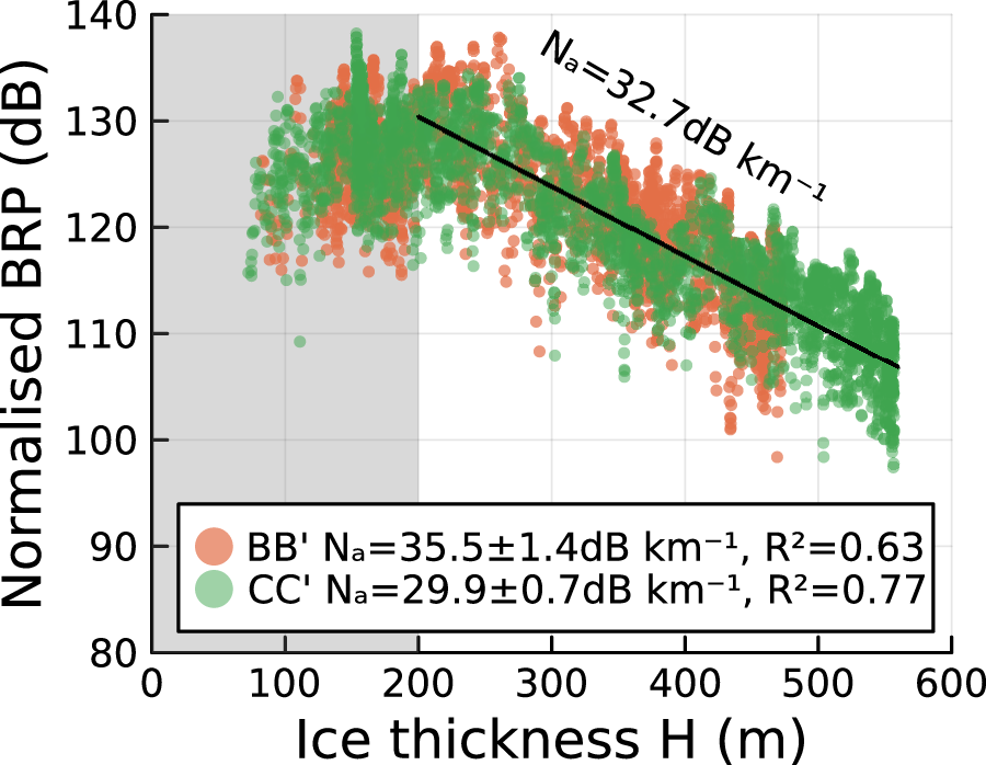


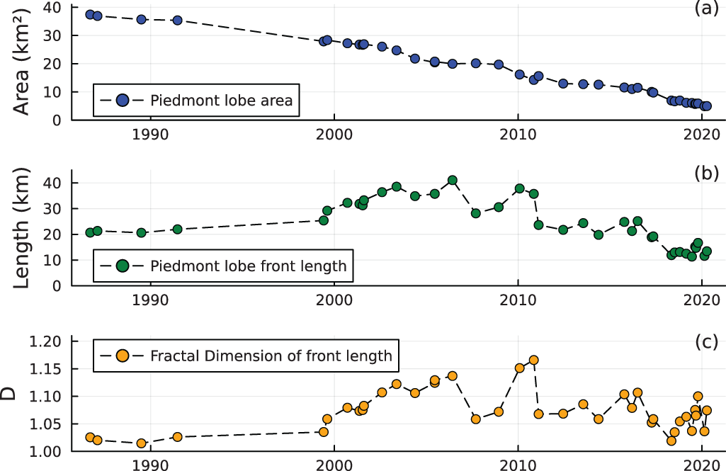
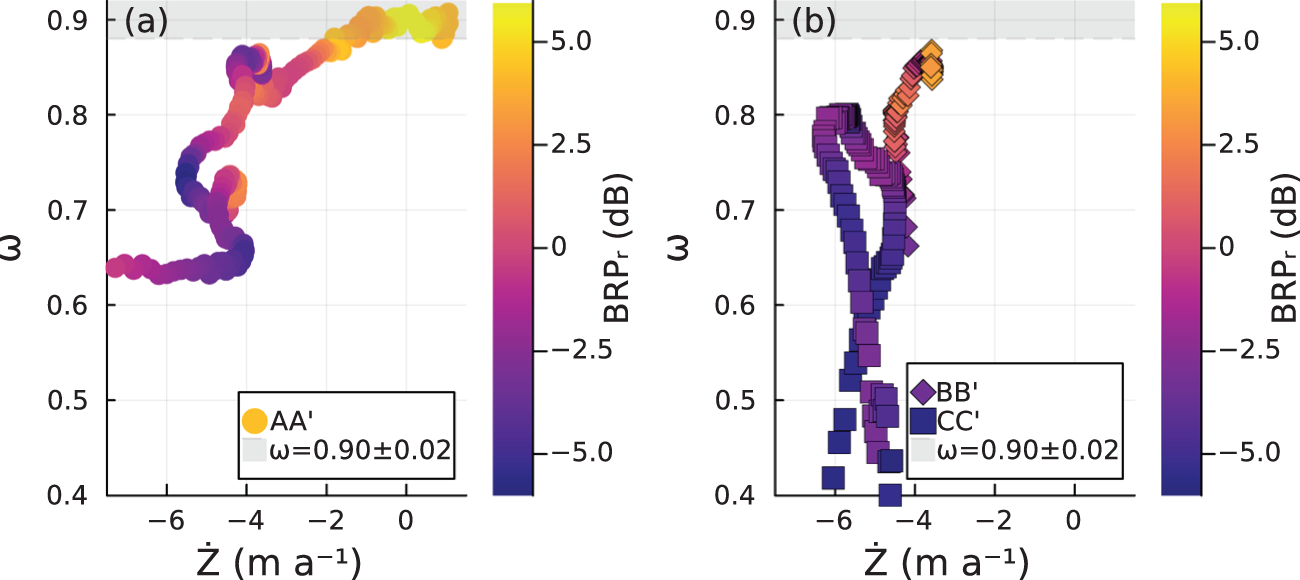


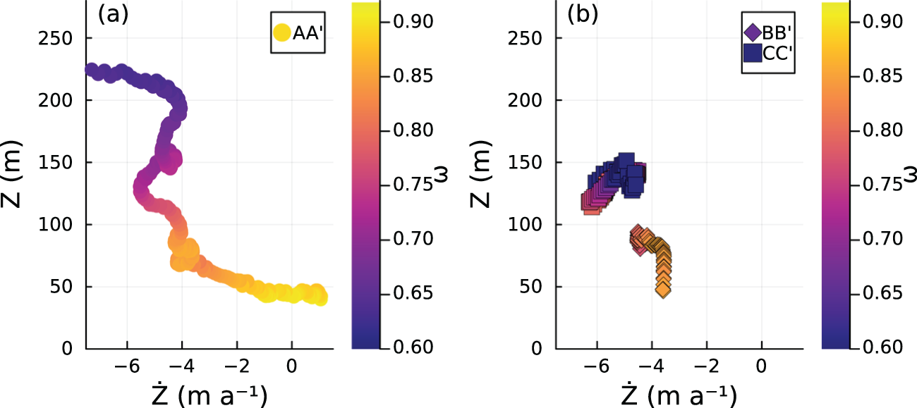


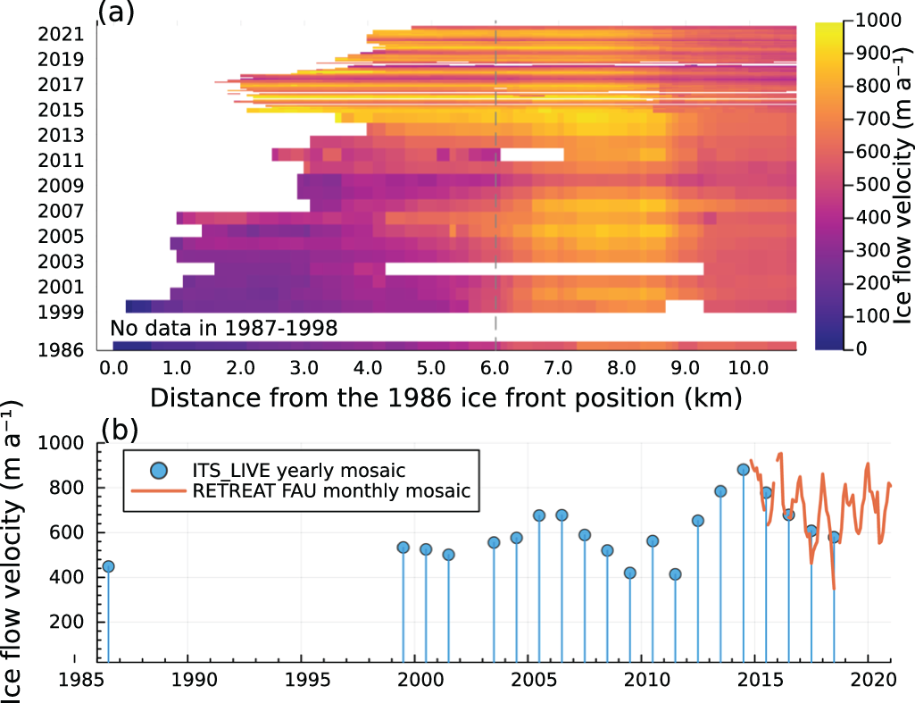


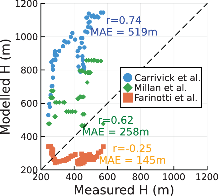


 Open access

