



1. Introduction
In this paper we study a threshold variant of the contact process, the threshold-one contact process, and two threshold variants of the voter model, the threshold-one voter model and the threshold-one voter model with spontaneous death, on homogeneous trees. The threshold contact process and the threshold voter model were first defined by Cox and Durrett in [Reference Cox and Durrett4]. Recall that for the contact process and the voter model, the interacting rate, i.e. the birth rate for the contact process and the flipping rates for the voter model, are linear functions with respect to the number of particles of different type in the neighborhood, denoted by N. In these variant models, these rates are replaced by a step function of N which jumps from 0 to  $\lambda$
at
 $N=\theta$
. For the threshold contact process with
 $\theta\ge 2$
the model has been studied in several works, including [Reference Mountford and Schonmann17]; for
 $\theta=1$
, [Reference Cox and Durrett4] proves a number of properties for the process on
 $\mathbb{Z}^d$
, including the complete convergence theorem, and [Reference Penrose19] studies the asymptotic behavior of the critical value for long interacting ranges. More recently, in [Reference Xue23], Xue revisits this case and calls it the ‘threshold-one contact process’. In [Reference Xue23], Xue shows that the critical birth/infection rate
 $\lambda$
for the threshold-one contact process on a high-dimensional lattice is
 ${\sim} \left(2d\right)^{-1}$
, where d is the dimension. Later, in [Reference Xue24], he shows the convergence rate when the system dies out. For the threshold voter model, [Reference Cox and Durrett4] raises several conjectures and proves that the complete convergence theorem holds for the threshold-one voter model with positive spontaneous death starting from the translation-invariant measure. Later, a number of works studying the threshold voter models on
 $\mathbb{Z}^d$
appeared, including [Reference Andjel, Liggett and Mountford2, Reference Handjani9, Reference Liggett14]. In particular, when
 $\theta=1$
and
 $\left(d,M\right)\ne\left(1,1\right)$
, [Reference Liggett14] proves the coexistence and [Reference Handjani9] proves the complete convergence theorem.
At the same time, although the contact process and its variants were originally studied on a lattice, they may also be defined on other finite or infinite graphs, including d-dimensional homogeneous trees  $\mathbb{T}_d$
. The behavior of the ordinary contact process on
 $\mathbb{T}_d$
differs from that on a lattice in the sense that there exists a second phase transition of strong/local survival which opens the possibility that the distribution of the process may still go to zero, even if the population itself persists; see [Reference Durrett and Schinazi7, Reference Liggett14, Reference Morrow, Schinazi and Zhang16, Reference Salzano and Schonmann20, Reference Stacey22] for details. Works such as [Reference Liggett12, Reference Liggett14, Reference Pemantle18, Reference Ziezold and Grillenberger26] give estimates for the upper and lower bounds for the critical values. When the ordinary contact process on
 $\mathbb{T}_d$
survives strongly, the complete convergence theorem was shown in [Reference Zhang25], while an alternative approach can be found in [Reference Liggett14, Reference Salzano and Schonmann20]. In [Reference Cranston, Mountford, Mourrat and Valesin5] and [Reference Stacey21], the process restricted on a finite subtree is also discussed. When
 $\theta=1$
, for the threshold-one contact process, [Reference Xue23] shows that the critical value is
 ${\sim} d^{-1}$
for large d. However, until now, little is known, to our knowledge, about the threshold voter model on
 $\mathbb{T}_d$
.
As discussed above, a particle system on homogeneous trees  $\mathbb{T}_d$
may exhibit a second phase transition of strong/local survival. To be precise, consider
 $\theta^{\lambda,\mathbb{T}_d}_t$
to be a translation-invariant interacting system on
 $\left\{0,1\right\}^{\mathbb{T}_d}$
that is monotone with respect to
 $\lambda$
and attractive with respect to the natural order on
 $\left\{0,1\right\}^{\mathbb{T}_d}$
. Denote by
 $\textbf{0}$
the configuration such that
 $\eta\left(x\right)\equiv 0$
for all
 $x\in\mathbb{T}_d$
, and by
 $\textbf{1}$
the configuration such that
 $\eta\left(x\right)\equiv 1$
for all
 $x\in\mathbb{T}_d$
. Without loss of generality, we can assume that
 $\theta^{\lambda,\mathbb{T}_d}_t$
is monotonically increasing with respect to
 $\lambda$
. Then, the different senses of survival/critical value(s) can be defined as follows (see [Reference Durrett and Schinazi7], for example):
•
 $\theta^{\lambda,\mathbb{T}_d}_t$
survives from a finite population if, for all x,
otherwise it dies out. We define the critical value as
\begin{equation*}\lim_{t\to\infty} \mathbb{P}^x\big(\theta^{\lambda,\mathbb{T}_d}_t\not=\textbf{0} \big)>0,\end{equation*}
\begin{equation*}\lambda_{\rm e}\left(d\right)=\inf\big\{\lambda\,{:}\,\theta^{\lambda,\mathbb{T}_d}_t \text{survives from a finite population}\big\}.\end{equation*}
•
$\theta^{\lambda,\mathbb{T}_d}_t$
survives if
where
\begin{equation*}\bar\nu^\lambda=\lim_{t\to\infty} \delta_\textbf{1} S^\lambda\left(t\right)\not=\delta_\textbf{0},\end{equation*}
$S^\lambda\left(\cdot\right)$
stands for the semigroup of
$\theta^{\lambda,\mathbb{T}_d}_t$
. We define the critical value as
\begin{equation*}\lambda_1\left(d\right)=\inf\big\{\lambda\,{:}\,\text{$\theta^{\lambda,\mathbb{T}_d}_t$ survives}\big\}.\end{equation*}
•
$\theta^{\lambda,\mathbb{T}_d}_t$
survives locally/strongly [Reference Durrett and Schinazi7, Reference Liggett13, Reference Morrow, Schinazi and Zhang16] if, for all x,
We define the critical value as
\begin{equation*} \mathbb{P}^x\left(\theta^{\lambda,\mathbb{T}_d}_t\left(x\right)=1 \ \text{infinitely often (i.o.)}\right)>0.\end{equation*}
\begin{equation*}\lambda_2\left(d\right)=\inf\left\{\lambda\,{:}\,\text{$\theta^{\lambda,\mathbb{T}_d}_t$ survives strongly}\right\}.\end{equation*}


2. Statement of main theorems
2.1. Results for the threshold-one contact process
Denote by  $\xi^{\lambda,\mathbb{T}_d}_t$
the threshold-one contact process on
 $\mathbb{T}_d$
. Observe that the system is increasing with respect to
 $\lambda$
, additive, and attractive with respect to the natural order of configurations, and that
 $\delta_{\textbf{0}}$
is the only absorbing state/trivial invariant distribution. Recalling the definitions of the different critical values, it is easy to see that
 $\lambda_2\left(d\right)\ge \max\left\{\lambda_1\left(d\right),\lambda_{\rm e}\left(d\right)\right\}$
. In Section 3 we will see that
 $\tilde \xi^{\lambda,\mathbb{T}_d}_t$
is the time reversal of
 $\xi^{\lambda,\mathbb{T}_d}_t$
, and thus
 $\tilde \xi^{\lambda,\mathbb{T}_d}_t$
survives from a finite population if and only if
 $\xi^{\lambda,\mathbb{T}_d}_t$
survives. Unlike the ordinary contact process which is self dual, it is clear that
 $\tilde \xi^{\lambda,\mathbb{T}_d}_t$
is not identically distributed as
 $\xi^{\lambda,\mathbb{T}_d}_t$
. So we first prove:
Theorem 1. For any  $\lambda>0$
,
 $\xi^{\lambda,\mathbb{T}_d}_t$
survives if and only if it survives from a finite population. This also implies that
 $\lambda_{\rm e}\left(d\right)=\lambda_1\left(d\right)$
.
With Theorem 1, we will no longer discriminate between survival and survival from a finite population, and from now on we denote such a condition by survival. The following two results give sufficient conditions for  $\xi^{\lambda,\mathbb{T}_d}_t$
to survive:
Theorem 2. For any  $d\ge 2$
,
 $\lambda_1\left(d\right)<1/\left(d-1\right)$
.
Remark 1. Recall that  $\lambda_1$
is the critical value for the existence of a nontrivial stationary distribution. [Reference Xue23, Corollary 3.2 and Theorem 4.1] proves that
 $1/\left(d+1\right)\le\lambda_1\left(d\right)\le1/\left(d-1\right)$
. With Theorem 1, one can see that Theorem 2 slightly improves the result by showing survival on the common upper bound.
Note that the condition of survival in Theorem 2 is not necessarily sharp for each given d, although it has been shown in [Reference Xue23] to be asymptotically sharp as  $d\to\infty$
. In fact, when
 $d=2$
,
 $\xi^{\lambda,\mathbb{T}_d}_t$
survives for substantially smaller
 $\lambda$
:
Theorem 3.  $\lambda_1\left(2\right)<0.637$
.
The following theorem gives an almost complete picture on the complete convergence theorem of the threshold-one contact process on  $\mathbb{T}_d$
. In words, the complete convergence theorem holds if and only if
 $\xi^{\lambda,\mathbb{T}_d}_t$
dies out or survives strongly. When the process survives weakly, we can prove the convergence theorem for any translation-invariant
 $\mu$
or Dirac measure concentrating on the dense configuration. Recall the definition of dense configuration in [Reference Griffeath8] such that
 $\xi$
is dense if it satisfies
 \begin{align} &\text{there exists } N>0 \text{ such that, for any } x\in\mathbb{T}_d,\nonumber\\[2pt] &\quad \text{there exists } y\in B_x\left(N\right) \text{such that } \xi\left(y\right)=1 , \end{align}
where  $B_x\left(N\right)$
is the ball of radius N centered at x. Note that the Dirac measure
 $\delta_\xi$
when
 $\xi$
is dense does not have to be translation invariant, and under the translation-invariant measure, the configuration
 $\xi$
does not have to be dense with probability one, so we need to give these two cases separately.
1. If
$\lambda>\lambda_2$
, for any initial configuration
$\xi$
,
(2.2)where
\begin{equation}\begin{aligned}\lim_{t\to\infty}\delta_{\xi} S^\lambda\left(t\right)= \left[1-\alpha_\xi \left(\lambda\right)\right]\bar \nu^\lambda+\alpha_\xi\left(\lambda\right) \delta_{\textbf{0}},\end{aligned}\end{equation}
$ \alpha_\xi\left(\lambda\right)=\mathbb{P}^{\xi}\left( {\xi}^{\lambda,\mathbb{T}_d}_t= \textbf{0}\text{ for some }t\right)$
,
$S^\lambda\left(t\right)$
is the Markov semigroup, and
$\bar\nu^\lambda $
is the maximal invariant measure of
${\xi}^{\lambda,\mathbb{T}_d}_t$
.2. If
$\lambda_1<\lambda\le\lambda_2$
, for any
$\mu$
that is translation invariant or has
$\mu=\delta_\xi$
where
$\xi$
is dense, we have
where
\begin{equation*}\lim_{t\to\infty}{\mu} S^\lambda\left(t\right)=\left[1- \alpha_\mu \left(\lambda\right)\right]\bar \nu^\lambda+\alpha_\mu\left(\lambda\right) \delta_{\textbf{0}},\end{equation*}
$ \alpha_\mu\left(\lambda\right)=\mathbb{P}^\mu\left(\xi=\textbf{0}\right)$
.3. If
$\lambda\le\lambda_1$
, for any initial configuration
$\xi$
,
\begin{equation*}\lim_{t\to\infty}\delta_{\xi} S^\lambda\left(t\right)=\delta_{\textbf{0}}.\end{equation*}








Remark 2. When  $\lambda_2\left(d\right)$
does not exist, the theorem makes no sense. In fact, similar to the ordinary contact process on
 $\mathbb{T}_d$
, we can prove that
 $\lambda_2\left(d\right)\le\frac{1}{\sqrt{d}-1}$
.
2.2. Results for the threshold-one voter model with positive spontaneous death
Denote by  $\eta_t^{\varepsilon,\mathbb{T}_d}$
the threshold-one voter model with positive spontaneous death rate
 $\varepsilon$
on
 $\mathbb{T}_d$
, where when
 $\varepsilon=0$
it is the threshold-one voter model. Observe that
 $\eta_t^{\varepsilon,\mathbb{T}_d}$
is monotone with respect to
 $\varepsilon$
and is attractive with respect to the natural order of configurations, so that with the definition of the three types of survivals, we can define three critical values with respect to
 $\varepsilon$
:
 \begin{equation*}\begin{aligned}&\varepsilon_1\left(d\right)=\sup\big\{\varepsilon\,{:}\,\text{$\eta^{\varepsilon,\mathbb{T}_d}_t$ survives}\big\}, \\[2pt] &\varepsilon_{\rm e}\left(d\right)=\sup\big\{\varepsilon\,{:}\,\text{$\eta^{\varepsilon,\mathbb{T}_d}_t$ survives from a finite population}\big\}, \\[2pt] &\varepsilon_2\left(d\right)=\sup\big\{\varepsilon\,{:}\,\text{$\eta^{\varepsilon,\mathbb{T}_d}_t$ survives strongly}\big\}.\end{aligned}\end{equation*}
Like the threshold-one contact process, we have  $\varepsilon_2\left(d\right)\le \max\left\{\varepsilon_1\left(d\right),\varepsilon_{\rm e}\left(d\right)\right\}$
. Because the dual process is not attractive, there is no clear indication to our knowledge whether
 $\varepsilon_1\left(d\right)=\varepsilon_{\rm e}\left(d\right)$
. Since
 $\eta^{\varepsilon,\mathbb{T}_d}_t$
can dominate the threshold-one contact process
 $\xi^{1,\mathbb{T}_d}_t$
, by Theorem 2 and Theorem 3, we can get that for any
 $d\ge 2$
,
 $\varepsilon_{\rm e}\left(d\right)>0$
and
 $\varepsilon_1\left(d\right)>0$
, and by Remark 2, one can prove that
 $\varepsilon_2\left(d\right)>0$
when
 $d\ge 5$
. Next, for the the threshold-one voter model with positive spontaneous death, we also have the corresponding complete convergence theorem.
1. If
$\varepsilon<\varepsilon_2$
, for any initial configuration
$\eta$
,
where
\begin{equation*}\lim_{t\to\infty}\delta_{\eta} S^\varepsilon\left(t\right)=\left[1- \alpha_\eta \left(\varepsilon\right)\right]\bar\nu^\varepsilon+\alpha_\eta\left(\varepsilon\right)\delta_{\textbf{0}},\end{equation*}
$ \alpha_\eta(\varepsilon)=\mathbb{P}^{\eta}( {\eta}^{\varepsilon,\mathbb{T}_d}_t= \textbf{0}\text{ for some }t)$
,
$S^\varepsilon\left(t\right)$
is the Markov semigroup, and
$\bar\nu^\varepsilon $
is the upper invariant measure of
${\eta}^{\varepsilon,\mathbb{T}_d}_t$
.2. If
$\varepsilon_1\ge\varepsilon\ge\varepsilon_2$
, for any
$\mu$
that is translation invariant or such that
$\mu=\delta_\eta$
where
$\eta$
is dense, we have
where
\begin{equation*}\lim_{t\to\infty}{\mu} S^\varepsilon\left(t\right)=\left[1- \alpha_\mu \right]\bar \nu^\varepsilon+\alpha_\mu \delta_{\textbf{0}},\end{equation*}
$ \alpha_\mu =\mu\left(\eta=\textbf{0}\right)$
.3. If
$\varepsilon>\varepsilon_1$
, for any initial configuration
$\eta$
, we have
\begin{equation*}\lim_{t\to\infty}\delta_{\eta} S^\varepsilon\left(t\right)= \delta_{\textbf{0}}.\end{equation*}








Next, we will consider the threshold-one voter model on  $\mathbb{T}_d$
; we denote the process by
 $\zeta^{\mathbb{T}_d}_{t}$
. Since
 $\zeta^{\mathbb{T}_d}_{t}$
can dominate the threshold-one contact process with parameter 1, by Theorems 2 and 3 and [Reference Liggett14, Proposition 2.11], we have:
Theorem 6. For any  $d\ge 2$
,
 $\zeta^{\mathbb{T}_d}_{t}$
coexists, i.e. there exists a nontrivial invariant measure.
Then, by Remark 2 and the domination of  $\xi^{\lambda,\mathbb{T}_d}_{t}$
, we can get that
 $\zeta^{\mathbb{T}_d}_{t}$
survives strongly when
 $d\ge 5$
.
Define  $\beta\left(d\right)=\lim\limits_{n\to\infty}\left[\mathbb{P}^o\left(x_n\in \zeta_t^{\mathbb{T}_d}\text{ for some }t\right)\right]^{1/n}$
. Then
 $\beta\left(d\right)$
exists by [Reference Liggett14, Theorem B22]. Like the definition in (2.1), we define the configuration to be doubly dense if it satisfies
 \begin{align} &\text{there exists } N>0 \text{ such that, for any } x\in\mathbb{T}_d, \nonumber\\[3pt] & \quad \text{ there exist } y,z\in B_x\left(N\right) \text{ such that } \zeta\left(y\right)=1,\ \zeta\left(z\right)=0.\end{align}
1. When
$\zeta_t^{\mathbb{T}_d}$
survives strongly, for any initial configuration
$\zeta$
,
where
\begin{equation*}\lim_{t\to\infty}\delta_{\zeta} U\left(t\right)= \alpha_\zeta\delta_0+\beta_\zeta\delta_1+\left(1-\alpha_\zeta-\beta_\zeta\right)\mu^d_{1/2} , \end{equation*}
$\alpha_\zeta=\mathbb{P}^\zeta( {\zeta}^{\mathbb{T}_d}_t= \textbf{0}\text{ for some }t)$
,
$\beta_\zeta=\mathbb{P}^\zeta( {\zeta}^{\mathbb{T}_d}_t= \textbf{1}\text{ for some }t)$
,
$U\left(t\right)$
is the Markov semigroup of
$\zeta_t^{\mathbb{T}_d}$
, and
$\mu^d_{1/2} $
is the limiting distribution of the process starting from the product distribution with parameter 1/2.2. When
$\beta\left(d\right)< \frac{1}{\sqrt{d}\,}$
, for any
$\mu$
that is translation invariant or such that
$\mu=\delta_\zeta$
where
$\zeta$
is doubly dense,
where
\begin{equation*}\lim_{t\to\infty}\mu U\left(t\right)= \alpha_{\mu}\delta_{\textbf{0}}+\beta_{\mu}\delta_{\textbf{1}}+\left(1- \alpha_{\mu}- \beta_{\mu}\right)\mu^d_{1/2},\end{equation*}
$\alpha_\mu=\mu\left(\zeta=\textbf{0}\right)$
,
$\beta_\mu=\mu\left(\zeta=\textbf{1}\right)$
.



3. Preliminaries and graphical representations
3.1. Preliminaries
To precisely define the particle system, let  $\mathbb{T}_d$
be the homogeneous tree where each vertex has
 $d+1$
neighbors. One can order
 $\mathbb{T}_d$
such that, for each vertex x, it has exactly one parent, denoted as
 $\overleftarrow{x}$
, and d children. At the same time, one can also label all the d children of each vertex by 1 to d according to this order. If a vertex x can be traced back to another vertex y through a path going up in the ‘family tree’, we call x the ancestor and y the descendant. For vertices
 $x,y\in \mathbb{T}_d$
, we write
 $x\sim y$
if y is a neighbor of x, and we use
 $|x-y|$
to denote the distance between x and y on
 $\mathbb{T}_d$
; in particular, when
 $x=o$
, we denote the distance between y and o as
 $|y|$
.
According to [Reference Liggett14, Part 1, Section 4], one may embed  $\mathbb{Z}$
into
 $\mathbb{T}_d$
by assigning consecutive integers to a doubly infinite connected lineage within
 $\mathbb{T}_d$
such that, for vertex x and y which are parent and child, we always have
 $l(y)=l(x)+1$
, where l(x) is the integer number assigned to vertex x. Thus, one can also see l(x) as the generation number of vertex x along this lineage, and denote by o the vertex with
 $l(x)=0$
. Also, for each
 $k\in \mathbb{Z}$
, denote by
 $x_k$
the vertex on this lineage with
 $l(x_k)=k$
. With generation numbers defined along one specific lineage, one can now discriminate all other vertices with the following finite sequence of integers: for each point
 $z\in \mathbb{T}_d$
, define
 $n_z\in \mathbb{Z}^+\cup \{0\}$
such that
 $x_{-n_z}$
is the most recent common ancestor of o and z. In particular, z is a descendent of o if and only if
 $n_z=0$
. If
 $z\not= x_{-n_z}$
, note that there is a unique simple path
 $\vec y$
from
 $x_{-n_z}$
to z denoted by
 $x_{-n_z}=y(0), y(1),\ldots, y(m_z)=z$
. Now define
 $\big(r(1),r(2),\ldots, r(m_z)\big)\in \{1,2,\ldots, d\}^{m_z}$
such that, for each i, y(i) is the r(i)th descendent of
 $y(i-1)$
. From the definitions above, one can see that each vertex
 $z\in \mathbb{T}_d$
now has a unique correspondence with
 $\big(n_z, r(1),r(2),\ldots, r(m_z)\big)$
, while
 $|z|=n_z+m_z$
. One may note that the discussion above also gives an explicit construction of the infinite homogeneous tree
 $\mathbb{T}_d$
.
For any  $A\subseteq \mathbb{T}_d$
, denote by
 $\xi_A$
the configuration in
 $\{0,1\}^{T_d}$
such that
 $\xi_A(x)=1$
if and only if
 $x\in A$
.
3.2. Coalescing duality
The graphical representation for the threshold-one contact process is shown in [Reference Liggett11, Chapter I, Section 6]. Since the threshold-one contact process is additive, it has coalescing duality. Now we construct the threshold-one contact process and its dual process as follows.
For any  $x\in \mathbb{T}_d$
, let
 $\big\{T_n^{x,\mathcal{N}_x}\big\}$
and
 $\{T_n^{x,\emptyset}\}$
be two independent Poisson flows with rate
 $\lambda$
and 1 respectively. Let
 $\mathcal{N}_x=\{y\,{:}\,|y- x|\le 1\}$
be the neighborhood of x. At each event time s of
 $T_n^{x,\mathcal{N}_x}$
we draw an arrow from y to x for every
 $y\in \mathcal{N}_x\backslash\{x\}$
, which can be thought of as the particle at y giving birth at x at time s. And at each event time s of
 $T_n^{x,\emptyset}$
put a
 $\delta$
at (x, s) where
 $\delta$
represents deaths. We say that there is an open path from (x, 0) to (y, t) if there is a pair of sequences
 $x_0=x,\dots,x_n=y$
and
 $s_0=0<s_1<\cdots< s_n<s_{n+1}=t$
such that:
• for
$1\leq m\leq n$
there is an arrow from
$x_{m-1}$
to
$x_{m}$
at time
$s_m$
;• for
$0\leq m\leq n$
there are no
$\delta$
s in
$\{x_m\}\times(s_{m},s_{m+1})$
.



To get the threshold-one contact process, for any  $A\subset \mathbb{T}_d$
, let
 \begin{equation*}\xi_t^{\lambda,A,\mathbb{T}_d}(x)=\textrm{1}_{\{\text{there is an open path from (\textit{z}, 0) to (\textit{x}, \textit{t}) for some $z\in A$}\}}.\end{equation*}
To get the dual process up to time t, reverse the directions of the arrows and time in the graph representation before time t: for any  $s\leq t$
, for any
 $B\subset \mathbb{T}_d$
, let
 \begin{equation*}\tilde{\xi}^{\lambda,B,\mathbb{T}_d}_{t,s}(x)=\textrm{1}_{\{\text{there is an open path from (\textit{z}, \textit{t}) to $(x,t-s)$ for some $z\in B$}\}}.\end{equation*}
Since for any  $s\leq t_1\leq t_2$
,
 $\tilde{\xi}^{\lambda,B,\mathbb{T}_d}_{t_1,s}$
and
 $\tilde{\xi}^{\lambda,B,\mathbb{T}_d}_{t_2,s}$
have the same distribution, we can define the dual process
 $\tilde{\xi}^{\lambda,B,\mathbb{T}_d}_{t}\triangleq\tilde{\xi}^{\lambda,B,\mathbb{T}_d}_{t,0}$
. Note that
 $\xi_t^{\lambda,A,\mathbb{T}_d}$
has the infinitesimal generator
 $\tilde\Omega^\lambda$
as follows: for any local function f,
 \begin{equation*}\Omega^\lambda f(\xi)=\sum_{x\in \mathbb{T}_d} \Bigg(\textrm{1}_{\{\xi\left(x\right)=1\}}[\,f\left(\xi^x\right)-f\left(\xi\right)]+ \lambda\textrm{1}_{\Big\{\xi\left(x\right)=0,\sum\limits_{y\sim x}\xi\left(y\right)\ge 1\Big\}} [\,f\left(\xi^x\right)-f\left(\xi\right)]\Bigg) ,\end{equation*}
where  $\xi^x$
has the same state as
 $\xi$
at any vertex except x. Also,
 $\tilde{\xi}^{\lambda,B,\mathbb{T}_d}_{t}(x)$
has the infinitesimal generator
 $\tilde\Omega^\lambda$
as follows: for any local function f,
 \begin{equation*}\tilde\Omega^\lambda f(\xi)=\sum_{x\in \mathbb{T}_d}\left( \textrm{1}_{\{\xi(x)=1\}}[\,f\left(\xi^ x\right)-f\left(\xi\right)]+ \lambda [\,f\left(\xi\cup \xi_{\mathcal{N}_x}\right)-f\left(\xi\right)]\right) ,\end{equation*}
where  $\xi\cup\eta=\xi\vee\eta$
.
Let  $\mathbb{P}^{\xi_A}(\cdot)$
and
 $\tilde{\mathbb{P}}^{\xi_B}(\cdot)$
denote the distribution of
 ${\xi}^{\lambda,A,\mathbb{T}_d}$
and
 $\tilde{\xi}^{\lambda,B,\mathbb{T}_d}$
respectively, and
 $\mathbb{E}^{\xi_A}(\cdot)$
and
 $\tilde{ \mathbb{E}}^{\xi_B}(\cdot)$
denote the corresponding expectations. When
 $A=\{x\}$
is a singleton, we abbreviate
 $\mathbb{P}^{\xi_{\{x\}}}$
,
 $\mathbb{E}^{\xi_{\{x\}}}$
, and
 ${\xi}^{\lambda,A,\mathbb{T}_d}$
to
 $\mathbb{P}^x$
,
 $\mathbb{E}^x$
, and
 ${\xi}^{\lambda,x,\mathbb{T}_d}$
for convenience, and we sometimes omit A in
 ${\xi}^{\lambda,A,\mathbb{T}_d}$
. From the construction, we can get the following important dual relation:
 \begin{equation}\begin{aligned} \mathbb{P}^{\xi_A} \big(\xi^{\lambda,\mathbb{T}_d}_t\cap\xi_B\ne \textbf{0}\big)=\tilde{\mathbb{P}}^{\xi_B} \big( \tilde{\xi}^{\lambda,\mathbb{T}_d}_t\cap \xi_A\ne\textbf{0} \big) \qquad \text{for all}\ A, B \subset \mathbb{T}_d , \end{aligned}\end{equation}
where  $\xi\cap\eta=\xi\land\eta$
.
The graph representation is a useful tool to get the monotonicity of  $\xi_t^{\lambda,\mathbb{T}_d}$
in
 $\lambda$
and the initial distribution such that:
• For any
$\lambda_{(1)}\leq\lambda_{(2)}$
, regarding the Poisson arrows with parameter
$\lambda_{(2)}$
as superpositions of independent Poisson arrows with parameter
$\lambda_{(1)}$
and
$\lambda_{(2)}-\lambda_{(1)}$
, we can couple
$\xi_t^{\lambda_{(1)},\mathbb{T}_d}$
and
$\xi_t^{\lambda_{(2)},\mathbb{T}_d}$
on the common graph representation, so that
for any t when both starting from A.
\begin{equation*}\begin{aligned} \xi_t^{\lambda_{(1)},\mathbb{T}_d}\subseteq \xi_t^{\lambda_{(2)},\mathbb{T}_d}\end{aligned}\end{equation*}
• For any finite subsets
$A\subseteq B$
, we can couple
${\xi}^{\lambda,A,\mathbb{T}_d}$
and
${\xi}^{\lambda,B,\mathbb{T}_d}$
with the same
$\lambda$
such that
for any t by using the same Poisson flows on a common graph representation.
\begin{equation*}\begin{aligned} \xi_t^{\lambda,A,\mathbb{T}_d}\subseteq \xi_t^{\lambda,B,\mathbb{T}_d}\end{aligned}\end{equation*}


The same results also hold for the dual process. Moreover,  $\xi^{\lambda,\mathbb{T}_d}_t$
and
 $\tilde \xi^{\lambda,\mathbb{T}_d}_t$
are additive in the sense that
 \begin{equation*}\xi^{\lambda,A,\mathbb{T}_d}_t=\cup_{x\in A}\xi^{\lambda,x,\mathbb{T}_d}_t, \qquad \tilde \xi^{\lambda,A,\mathbb{T}_d}_t=\cup_{x\in A}\tilde \xi^{\lambda,x,\mathbb{T}_d}_t.\end{equation*}
Let  $A=\mathbb{T}_d$
in (3.1); we obtain
 \begin{equation*}\tilde{\mathbb{P}}^{\xi_B}\big(\tilde{\xi}^{\lambda,\mathbb{T}_d}_t\ne\textbf{0}\big)=\delta_\textbf{1}S^\lambda(t)(\xi\,{:}\,\xi\cap \xi_B\ne\textbf{0}).\end{equation*}
Thus, the limit of  $\delta_\textbf{1}S^\lambda(t)$
exists; denote it as
 $\bar{\nu}^\lambda$
, such that
 \begin{equation}\begin{aligned}\tilde{\mathbb{P}}^{\xi_B}\big(\tilde{\xi}^{\lambda,\mathbb{T}_d}_t\ne\textbf{0}\text{ for all}\ t\big)=\bar{\nu}^\lambda(\xi\,{:}\,\xi\cap \xi_B\ne\textbf{0})\end{aligned}\end{equation}
for any B.
3.3. Annihilating duality
Since the threshold-one voter model is not additive, it has no coalescing duality. However, it has another important duality, the annihilating duality (see [Reference Liggett11, Chapter 3.4]), which was introduced in [Reference Cox and Durrett4].
For any  $x\in \mathbb{T}_d$
, let
 $\{T_n^{x,S_x}\}_{S_x\subseteq \mathcal{N}_x}$
and
 $\{T_n^{x,\emptyset}\}$
be independent Poisson processes with rate
 $\beta(S_x)$
and
 $\varepsilon$
respectively, where
 \begin{equation*} \beta(S_x)= \left \{ \begin{array}{l@{\quad}l} \frac{1}{2^{d}}, \quad &S_x\subset\mathcal{N}_x \text{ and $|S_x|\ge 2$ is even,}\\[3pt] 0,\quad & \text{otherwise}. \end{array}\right.\\\end{equation*}
At any event time  $t\in\{T_n^{x,S_x}\}$
draw an arrow from y to x for every
 $y\in S_x$
, and if
 $x\in S_x$
put a
 $\delta$
at (x, t), while if
 $t\in\{T_n^{x,\emptyset}\}$
, put a
 $\delta$
at (x, t).
Let  $\eta_t^{\varepsilon,A,\mathbb{T}_d}(x)=\textrm{1}_{\{\text{there are an odd number of paths from}\ (z,\ 0)\ to\ (x,\ t)\ \text{for some }\ z\ \in\ A \}}$
. Reverse the direction of the arrows, let
 \begin{equation*}\begin{aligned} \tilde{\eta}_{t,s}^{\varepsilon,B,\mathbb{T}_d}(y)=\textrm{1}_{\{\text{there are an odd number of paths from (\textit{z}, \textit{t}) to (\textit{y}, \textit{s}) for some $z\in B$}\}}.\end{aligned}\end{equation*}
Then the dual process starting from  $\eta_B$
can be defined as
 $\tilde{\eta}_{t,0}^{\varepsilon,B,\mathbb{T}_d}$
. From the above argument we can define the infinitesimal generator of
 $\eta_t^{\varepsilon,A,\mathbb{T}_d}$
as: for any local function f,
 \begin{equation*}\Omega^\varepsilon f(\eta)=\sum_{x\in \mathbb{T}_d}\Bigg(\sum_{S_x} \beta\left(S_x\right)[\,f\left(\eta\triangle \eta_{S_x}\right)-f\left(\eta\right)]+\varepsilon\textrm{1}_{\{\eta(x)=1\}}\big[\,f\left(\eta^x\right)-f\left(\eta\right)\big]\Bigg) ,\end{equation*}
where  $\eta\triangle \eta_{S_x}(y)=1$
if and only if
 $\eta(y)[1-\eta_{S_x}(y)]=1$
or
 $[1-\eta(y)]\eta_{S_x}(y)=1$
 $\eta$
being odd means that there are an odd number of 1s in
 $\eta$
.
Also, the infinitesimal generator of  $\tilde\eta_t^{\varepsilon,A,\mathbb{T}_d}$
can be defined as: for any local function f,
 \begin{equation*}\tilde\Omega^\varepsilon f(\eta)=\sum_{x\in \mathbb{T}_d}\Bigg(\sum_{S_x} \beta\left(S_x\right)[\,f\left(\eta\triangle \eta_{S_x}\right)-f\left(\eta\right)]+\varepsilon\textrm{1}_{\{\eta\left(x\right)=1\}}\big[\,f\left(\eta^x\right)-f\left(\eta\right)\big]\Bigg).\end{equation*}
The threshold-one voter model is the special case when  $\varepsilon=0$
.
From the construction above,  ${\eta}^{\varepsilon,\mathbb{T}_d}_t$
and
 $\tilde{\eta}^{\varepsilon,\mathbb{T}_d}_t$
can be seen as annihilating branching processes in the sense that when two particles meet, they annihilate. Thus, we get the duality relation:
 \begin{equation}\begin{aligned}\mathbb{P}^{\eta_A}\big( \eta_t^{\varepsilon,\mathbb{T}_d}\cap \eta_B\text{ is odd} \big)=\tilde{\mathbb{P}}^{\eta_B}\big( \tilde{\eta}_t^{\varepsilon,\mathbb{T}_d}\cap \eta_A\text{ is odd} \big) \qquad \text{for all}\ A, B.\end{aligned}\end{equation}
4. The threshold-one contact process
The proofs in this section are mostly adaptions of the corresponding results and methods developed for the ordinary contact process on  $\mathbb{T}_d$
, in particular those in [Reference Liggett13] and [Reference Liggett14].
4.1. Equivalence of survivals
In this subsection we extend the arguments in [Reference Liggett14, Part I, Section 4] to  $\xi^{\lambda,\mathbb{T}_d}_t$
and
 $\tilde \xi^{\lambda,\mathbb{T}_d}_t$
with
 $\rho=1$
and prove Theorem 1. The proofs of Lemmas 1 and 2 are parallel, with no significant difference from those in [Reference Liggett14] since all three processes
 $\xi^{\lambda,\mathbb{T}_d}_t$
,
 $\tilde \xi^{\lambda,\mathbb{T}_d}_t$
, and the ordinary contact process are attractive and additive spin systems, so we omit the proofs here.
Lemma 1. (Adaption of Proposition 4.27(b), [Reference Liggett14])
 \begin{equation}\begin{aligned}\Phi\left(\lambda\right)=\lim\limits_{t\to\infty}\mathbb{E}^o|\xi^{\lambda,\mathbb{T}_d}_t|^{1/t}\end{aligned}\end{equation}
exists, and there exists  $ C<\infty$
such that
 \begin{equation*}\begin{aligned} \left[\Phi\left(\lambda\right)\right]^t\leq \mathbb{E}^o|\xi^{\lambda,\mathbb{T}_d}_t|\leq C\left[\Phi\left(\lambda\right)\right]^t.\end{aligned}\end{equation*}
Lemma 2. (Adaption of Proposition 4.39, [Reference Liggett14])
 \begin{equation}\begin{aligned}&\lambda_{\rm e}\left(d\right)=\sup\{\lambda\,{:}\,\Phi\left(\lambda\right)\leq1\},\\[2pt] &\tilde{\lambda}_{\rm e}\left(d\right)=\sup\{\lambda\,{:}\,\tilde{\Phi}\left(\lambda\right)\leq1\}.\end{aligned}\end{equation}
Moreover,  $\xi^{\lambda,\mathbb{T}_d}_t$
and
 $\tilde\xi^{\lambda,\mathbb{T}_d}_t$
die out at the first critical value.
Proof of Theorem 1. By duality, it suffices to prove  $\lambda_{\rm e}\left(d\right)=\tilde{\lambda}_{\rm e}\left(d\right)$
. When starting from a single vertex
 $o$
, it is easy to calculate that
 \begin{equation}\begin{aligned}\mathbb{E}^o|\xi^{\lambda,\mathbb{T}_d}_t|=\sum\limits_{n=0}^{\infty}\left(d+1\right)d^n\mathbb{P}^o\big(x_n\in \xi^{\lambda,\mathbb{T}_d}_t\big)=\sum\limits_{n=0}^{\infty}\left(d+1\right)d^n\mathbb{P}^o\big(x_n\in \tilde{\xi}^{\lambda,\mathbb{T}_d}_t\big)=\mathbb{E}^o|\tilde{\xi}^{\lambda,\mathbb{T}_d}_t|.\end{aligned}\end{equation}
By the definition of  $\Phi$
in (4.1),
 $\Phi\left(\lambda\right)=\tilde{\Phi}\left(\lambda\right)$
. Thus, it follows from (4.2) that
 $\lambda_{\rm e}\left(d\right)=\tilde{\lambda}_{\rm e}\left(d\right)$
. Moreover, by Lemma 2, both
 $\xi^{\lambda,\mathbb{T}_d}_t$
and
 $\tilde{\xi}^{\lambda,\mathbb{T}_d}_t$
die out at the first critical value, so
 $\xi^{\lambda,\mathbb{T}_d}_t$
neither survives nor survives from a finite population at
 $\lambda_{\rm e}\left(d\right)$
by duality.
Remark 3. Define another two critical values:
 \begin{align*}&\lambda_{\rm T}=\sup\left\{\lambda\,{:}\left(\int_0^\infty\mathbb{E}^o|\xi^{\lambda,\mathbb{T}_d}_t|\,{\rm d} t\right)<\infty\right\},\\[3pt] &\tilde\lambda_{\rm T}=\sup\left\{\lambda\,{:}\left(\int_0^\infty\mathbb{E}^o|\tilde\xi^{\lambda,\mathbb{T}_d}_t|\,{\rm d} t\right)<\infty\right\}.\end{align*}
Then, by (4.3), we get  $\lambda_{\rm T}=\tilde\lambda_{\rm T}$
. Once we have
 \begin{equation}\begin{aligned}\lambda_{\rm e}=\lambda_{\rm T}, \qquad \tilde\lambda_{\rm e}=\tilde\lambda_{\rm T},\end{aligned}\end{equation}
Theorem 1 holds immediately. For any transitive graph with bounded degree, [Reference Aizenman and Jung1] showed that for the ordinary contact process  $\hat\lambda_{\rm e}=\hat\lambda_{\rm T}$
, where
 $\hat\lambda_{\rm e}, \hat\lambda_{\rm T} $
represent the corresponding critical values for the ordinary contact process. Applying their proof to the threshold-one contact process and its dual process, we should also be able to obtain (4.4). Thus, Theorem 1 holds for any transitive graph with bounded degree, such as
 $\mathbb{Z}^d$
.
4.2. Conditions for survival
In this subsection we will give conditions for the dual process  $\tilde\xi^{\lambda_d,\mathbb{T}_d}_t$
to survive; as a result, we can get an upper bound for the critical value
 $\lambda_1\left(d\right)$
.
Proof of Theorem 2. For any non-empty  $A\in Y$
, define
 $g\left(A\right)=|A|$
. Then, for
 $\lambda_d=\left(d-1\right)^{-1}$
and our process
 $\xi^{\lambda_d,\mathbb{T}_d}_t$
on
 $\mathbb{T}_d$
, we can similarly define
 \begin{equation*}\begin{aligned}h^{\lambda_d}\left(A\right)&=\frac{{\rm d}}{{\rm d} t}\mathbb{E}^{\xi_A} \left[g\left(\xi^{\lambda_d,\mathbb{T}_d}_t\right)\right]\Big|_{t=0}\\[2pt] &=\lambda_d |\partial A|-|A|\\[2pt] &\ge \frac{1}{d-1}\left[\left(d-1\right)|A|+2\right]-|A|\\[2pt] &=\frac{2}{d-1}.\end{aligned}\end{equation*}
The third inequality comes from the fact that  $|\partial A|\ge\left(d-1\right)|A|+2$
, which can be proved by induction. First, when
 $|A|=1$
,
 $|\partial A|=d+1=\left(d-1\right)|A|+2$
. Then we assume that the inequality is true for all
 $|A|\le n-1$
. We come to the case when
 $|A|=n$
. Assume
 $x\in A$
has the maximum generation, i.e.
 $m_{x}-n_{x}=\max\left\{m_y-n_y\,{:}\,y\in A\right\}$
. If there is more than one such point, we choose the ‘smallest’ one according to the lexicographical order of
 $\left(n_z, r\left(1\right),r\left(2\right),\ldots, r\left(m_z\right)\right)$
. It follows that
 \begin{equation*} |\partial A|\ge |\partial \left(A\cup\left\{x\right\}\right)|-1+d ,\end{equation*}
where the inequality holds if and only if  $\overleftarrow x \in A$
. Hence, by the inductive hypothesis we have
 \begin{align*} |\partial A|&\ge |\partial \left(A\cup\left\{x\right\}\right)|-1+d \\[2pt] &\ge\left(d-1\right)\left(n-1\right)+2+d-1 \\[2pt] &=n\left(d-1\right)+2 \\[2pt] &=\left(d-1\right)|A|+2. \end{align*}
Now the fact is true for all A satisfying  $|A|=n$
and thus for all finite subsets A. From the transition rates above, one can see that the stochastic process
 $|\xi^{\lambda_d,\mathbb{T}_d}_t|$
dominates a Markov process
 $\hat A^d_t$
on
 $\mathbb{Z}^+\cup\left\{0\right\}$
with 0 as absorbing state and transition rates as follows: for each
 $n\in \mathbb{Z}^+$
,
 \begin{equation*}\left\{\begin{aligned}&n\rightarrow n+1 \text{ at rate } n+\tfrac{2}{d-1},\\&n\rightarrow n-1 \text{ at rate } n.\\\end{aligned}\right.\end{equation*}
Note that in Lemma 2 we have proved that survival of  $A^{\lambda_{d},\mathbb{T}_d}_t$
is equivalent to
 $\Phi\left(\lambda\right)>1$
. Define
 $\mathbb{E}^n$
as the expectation of a random walk starting from n. By Lemmas 1 and 2 it suffices to prove that
 $\lim\limits_{t\to\infty}\mathbb{E}^o\left|A^{\lambda_d,\mathbb{T}_d}_t\right|= \infty$
, which, by the discussion above, is immediate if one can show that
 \begin{equation}\begin{aligned}\lim_{t\to\infty}\mathbb{E}^1\left|\hat A^{d}_t\right|= \infty.\end{aligned}\end{equation}
Again, note that for  $\hat A^d_t$
, its infinitesimal mean is given by
 \begin{equation*}\mu^d\left(n\right)=\frac{{\rm d}}{{\rm d} t} \mathbb{E}^n \hat A^d_t\Big|_{t=0}=\frac{2}{d-1}\textrm{1}_{\left\{n\not=0\right\}}.\end{equation*}
Recalling that 0 is absorbing for  $\hat A^d_t$
, for stopping time
 $\hat \tau_0=\inf\big\{t\,{:}\,\hat A^d_t=0\big\}$
and any
 $t\in \left(0,\infty\right)$
, by Dynkin’s formula,
 \begin{equation*}\begin{aligned}\mathbb{E}^1 \hat A^d_t= 1+\mathbb{E}^1\left[\int_0^t \frac{2}{d-1}\textrm{1}_{\left\{\hat \tau_0>s\right\}}\,{\rm d} s \right]=1+ \frac{2}{d-1}\int_0^t \mathbb{P}^1\big(\hat \tau_0>s\big)\,{\rm d} s.\end{aligned}\end{equation*}
Note that  $\int_0^\infty \mathbb{P}^1\big(\hat \tau_0>s\big)\,{\rm d} s=\mathbb{E}^1\left[\hat \tau_0\right]$
, thus in order to prove (4.5), it is sufficient to prove that
 $\mathbb{E}^1\left[\hat \tau_0\right]=\infty$
.
Moreover, note that  $\hat A^d_t$
further dominates
 $S_t$
, a (inhomogeneously) rescaled continuous-time simple random walk with 0 as absorbing state and transition rates as follows: for each
 $n\ge 1$
,
 \begin{equation*}\frac{{\rm d}}{{\rm d} t} \mathbb{P}^n\left(S_t=n+1\right)\Big|_{t=0}=\frac{{\rm d}}{{\rm d} t} \mathbb{P}^n\left(S_t=n-1\right)\Big|_{t=0}=n.\end{equation*}
Let  $\tau_0=\inf\left\{t\,{:}\,S_t=0\right\}$
. Thus, we only need to prove that
 $\mathbb{E}^1\left[\tau_0\right]=\infty$
. Now define the following sequence of stopping times for
 $S_t$
:
 \begin{equation*}\tau_n=\inf\left\{t\ge 0\,{:}\,S_t=n\right\} \qquad \text{for all}\ n\ge 1,\end{equation*}
with the convention  $\inf\emptyset=\infty$
, and disjoint events
 $A_n=\left\{\tau_n<\infty, \ \tau_{n+1}=\infty\right\}$
. Then
 \begin{equation*}\begin{aligned}\mathbb{E}^1\left[\tau_0\right]=\sum_{n=1}^\infty \mathbb{E}^1\left[\tau_0\textrm{1}_{A_n}\right].\end{aligned}\end{equation*}
Now, for each sufficiently large n, note that on the event  $A_n$
,
 $\tau_n<\tau_0<\tau_{n+1}=\infty$
, which implies that
 \begin{equation}\begin{aligned}\mathbb{E}^1\left[\tau_0\textrm{1}_{A_n}\right]\ge \mathbb{E}^1\left[\tau_n\textrm{1}_{A_n}\right].\end{aligned}\end{equation}
Also, by the strong Markov property,
 \begin{equation}\begin{aligned}\mathbb{E}^1\left[\tau_n\textrm{1}_{A_n}\right]=\mathbb{E}^1\left[\tau_n\textrm{1}_{\left\{\tau_n<\infty\right\}}\right]\mathbb{P}^n\left(\tau_0<\tau_{n+1}\right)=\frac{1}{n+1} \mathbb{E}^1\left[\tau_n\textrm{1}_{\left\{\tau_n<\infty\right\}}\right],\end{aligned}\end{equation}
where the last equality is a result that the embedded chain of  $S_t$
is a simple random walk with 0 as absorbing state.
Now define  $Y_n$
as the number of transitions within
 $\left[0,\tau_n\wedge \tau_0\right]$
, and let
 $X_n$
,
 $n\ge 0$
, be a discrete simple random walk on
 $\mathbb{Z}$
with stopping time
 \begin{equation*}T_n=\min\left\{k\,{:}\,X_k=n\right\} \qquad \text{for all}\ n\ge 0.\end{equation*}
Then, again by the fact that the embedded chain of  $S_t$
is a simple random walk with 0 as absorbing state, we have, for all
 $m\ge 1$
,
 \begin{equation}\begin{aligned}\mathbb{P}^1(\tau_n<\infty, Y_n\ge m)=\mathbb{P}^1(T_n<T_0, T_n\ge m).\end{aligned}\end{equation}
Note that  $\mathbb{P}^1(T_n<T_0)=n^{-1}$
, while
 \begin{equation*}\mathbb{P}^1(T_n<m)= \mathbb{P}^0(T_{n-1}<m)\le \mathbb{P}^0\bigg(\max_{i\le m}X_i\ge n-1 \bigg).\end{equation*}
By the reflection principle,
 \begin{equation*}\mathbb{P}^0\bigg(\max_{i\le m} X_i\ge n-1 \bigg)=2 \mathbb{P}^0(X_m\ge n-1).\end{equation*}
Now let  $m_n=\left[n^2/\left(3\log n\right)\right]$
; by Chernoff’s inequality,
 \begin{equation*}\begin{aligned} \mathbb{P}^0\big(X_{m_n}\ge n-1\big)\le \exp\bigg(-\frac{\left(n-1\right)^2}{m_n}\bigg)\le \exp\left(-2\log n\right)=\frac{1}{n^2},\end{aligned}\end{equation*}
which implies that
 \begin{equation*}\mathbb{P}^1(T_n<T_0, T_n\ge m_n)\ge \mathbb{P}^1(T_n<T_0)-\mathbb{P}^1(T_n<m_n)\ge \frac{1}{n}-\frac{2}{n^2}\ge \frac{1}{2n}\end{equation*}
when n is large enough. At the same time, note that, given any nonzero and nearest-neighbor trajectory  $1=x_{\left(0\right)}, x_{\left(1\right)}, \ldots, x_{\left(m\right)}=n$
with
 $x_{\left(0\right)}, x_{\left(1\right)}, \ldots, x_{\left(m-1\right)}\in \left[1,n-1\right]$
as the embedded chain of
 $S_t$
within
 $\left[0,\tau_n\right]$
, the conditioned expectation of
 $\tau_n$
is given by
 \begin{equation*}\frac{1}{x_{\left(0\right)}}+\frac{1}{x_{\left(1\right)}}+\cdots+\frac{1}{x_{\left(m-1\right)}}\ge \frac{m}{n}.\end{equation*}
Moreover, in the event  $\left\{\tau_n<\infty, Y_n\ge m_n\right\}$
, each trajectory of the embedded chain within
 $\left[0,\tau_n\right]$
has to satisfy the condition above with
 $m=m_n$
. Thus,
 \begin{equation}\begin{aligned}\mathbb{E}\left[\tau_n \mid \tau_n<\infty, Y_n\ge m_n\right]\ge \frac{m_n}{n}\ge \frac{n}{4\log n}.\end{aligned}\end{equation}
By (4.6), (4.7), (4.8), and (4.9) we have
 \begin{align*}\mathbb{E}^1\left[\tau_0\textrm{1}_{A_n}\right] & \ge \frac{1}{n+1} \mathbb{E}^1\left[\tau_n\textrm{1}_{\left\{\tau_n<\infty\right\}}\right] \\ & \ge \frac{1}{n+1} \mathbb{P}^1(\tau_n<\infty, Y_n\ge m_n)\, \mathbb{E}\left[\tau_n \mid \tau_n<\infty, Y_n\ge m_n\right]\\& \ge \frac{1}{8\left(n+1\right)\log n}\end{align*}
when n is large enough, which is unsummable. Thus,  $\mathbb{E}^1[\tau_0]=\infty$
and the proof of Theorem 2 is complete.
Idea of the proof of Theorem 3 Recall that in Theorem 1 we have proved that  $\xi^{\lambda,\mathbb{T}_d}_t$
survives if and only if
 $\tilde{\xi}^{\lambda,\mathbb{T}_d}_t$
survives, and in Lemma 2 we proved that
 ${\xi}^{\lambda_1\left(2\right),\mathbb{T}_d}_t$
dies out. Thus, it suffices to prove that when
 $d=2$
and
 $\lambda\geq 0.637$
, the dual process
 $\tilde{\xi}^{\lambda,\mathbb{T}_d}_t$
survives. The constant
 $0.637$
is the same as the weaker upper bound for survival of the ordinary contact process on
 $\mathbb{T}_2$
found in [Reference Liggett13]. The key ingredient in this proof is to show that in the finite system, although
 $\tilde \xi^{\lambda,\mathbb{T}_d}_t$
and the ordinary contact process have different transition dynamics, their infinitesimal generators will behave exactly the same when applied to the special limiting test function f defined in [Reference Liggett13]. Specifically,
 \begin{equation*} h\left(A\right)=\frac{{\rm d}}{{\rm d} t}\mathbb{E}^{\xi_A}f\big(\tilde{A}^\lambda_t\big)\Big|_{t=0} \end{equation*}
is the same as [Reference Liggett13, (4.2)], which corresponds to the ordinary contact process.
Let  $\tau_a=\inf\left\{t\,{:}\,f\left(\xi_t^A\right)\le a\right\}$
where a is large enough. As a result, we can show that, for any finite set A,
 $f\Big(\tilde{\xi}^{\lambda,A,\mathbb{T}_d}_{t\land\tau_a}\Big)^{-1}$
is a nonnegative supermartingale whose transition rate has a uniform lower bound when
 $\lambda\geq 0.637$
. Applying the optional stopping theorem, we obtain that
 $\mathbb{P}^{\xi_A}\left(\tau_{a}=\infty\right)>0$
when
 $f\left(A\right)>a$
. Since
 $f\left(\textbf{0}\right)=0$
, we get
 $\mathbb{P}^{\xi_A}\left(\tau_{\textbf{0}}=\infty\right)>0$
. So we have proved that
 $\tilde{\xi}^{\lambda,\mathbb{T}_d}_t$
survives when
 $\lambda\geq 0.637$
. Since the approach follows that in [Reference Liggett13, Theorem 1.2(a)], for completeness we put the detailed proof in Appendix A.
4.3. Results for strong survival
It is easy to generalize some results for the ordinary contact process on  $\mathbb{T}_d$
, which are proved in [Reference Liggett14], to all attractive spin systems we consider in this paper (see Remark 4). For convenience, we just prove some for the threshold-one contact process.
Let  $\mathbb{T}^d_x$
be the subtree containing x together with all its descendants, and
 $\hat{\mathbb{T}}^d_x=\left(\mathbb{T}_d\backslash\mathbb{T}^d_x\right)\cup\left\{x\right\}$
. Denote by
 $\xi^{\lambda,\hat{\mathbb{T}}^d_x}_t$
the process restricted on
 $\hat{\mathbb{T}}^d_x$
which is always 0 outside. Define
 \begin{equation*}\beta\left(\lambda,d\right)=\lim\limits_{n\to\infty}\left[\mathbb{P}^o\big(x_n\in\xi^{\lambda,\mathbb{T}_d}_t \text{ for some }t\big)\right]^{1/n} ; \end{equation*}
this exists by [Reference Liggett14, Theorem B22].
Among the key statements proven below is
Lemma 3. (Adaption of Proposition 4.57, [Reference Liggett14]) If  $\beta\left(\lambda,d\right)>\frac{1}{\sqrt{d}\,}$
, then
 \begin{equation*}\inf\limits_t \mathbb{P}^o\Big(o\in \xi^{\lambda,\mathbb{T}^d_o}_t\Big)>0.\end{equation*}
Since the proof follows the approach used in [Reference Liggett14, Proposition 4.57], for completeness we put it in Appendix B.
Once we have Lemma 3, we immediately have the next three lemmas.
Lemma 4.  $ \mathbb{P}^o\Big(o\in \xi^{\lambda,\mathbb{T}_d}_t \text{ i.o.}\Big)>0\text{ if and only if }\inf_t \mathbb{P}^o\Big(o\in \xi^{\lambda,\mathbb{T}_o^d}_t\Big)>0$
.
Proof. When  $\inf_t\mathbb{P}^o\big(o\in \xi^{\lambda,\mathbb{T}^d_o}_t\big)>0$
,
 $\mathbb{P}^o\big(o\in \xi^{\lambda,\mathbb{T}_o^d}_t\text{ i.o.}\big)>0$
is immediate simply by definition. To prove the other direction, when
 $\mathbb{P}^o\big(o\in \xi^{\lambda,\mathbb{T}_d}_t\text{ i.o.}\big)>0$
, by a simple argument, we have
 \begin{equation*}\mathbb{P}^o\big(x_n\in \xi^{\lambda,\mathbb{T}_d}_t \text{ i.o.}\big)=\mathbb{P}^o\big(o\in \xi^{\lambda,\mathbb{T}_d}_t\text{ i.o.}\big)\qquad \text{for all}\ n\ge 1.\end{equation*}
Recalling the definition of  $\beta\left(\lambda,d\right)$
,
 \begin{equation*}\beta\left(\lambda,d\right)\ge \lim_{n\to\infty}\left[\mathbb{P}^o\big(x_n\in \xi^{\lambda,\mathbb{T}_d}_t \text{ i.o.}\big)\right]^{1/n}=1>\frac{1}{\sqrt{d}\,}.\end{equation*}
Thus, from Lemma 3 we have proved the other direction.
Lemma 5. When  $\mathbb{P}^o\big(o\in\xi^{\lambda,\mathbb{T}^d}_t\text{ i.o.}\big)>0$
,
 \begin{equation*}\lim\limits_{n\to\infty}\sup_t\mathbb{P}^{\xi_{B\left(n\right)}}\left(|\xi_t^{\lambda,\mathbb{T}_d}\cap B\left(n\right)|\le k\right)= 0 \qquad \text{for any } k,\end{equation*}
where  $B\left(n\right)$
is the ball of radius n centered at o.
Proof. By Lemma 4,
 \begin{equation*}\inf_{t\ge 0}\mathbb{P}^o\left(o\in\xi_t^{\lambda,\mathbb{T}^d_o}\right)\ge p>0.\end{equation*}
Since  $\mathbb{T}^d_x\cap\mathbb{T}^d_y=\emptyset$
for any
 $ x\ne y$
but
 $|x|=|y|$
,
 $\xi_t^{\lambda,\mathbb{T}^d_x}$
and
 $\xi_t^{\lambda,\mathbb{T}^d_y}$
are independent, so that, for any k,
 \begin{align*}\sup_t\mathbb{P}^{\xi_{B\left(n\right)}}\left(\big|\xi_t^{\lambda,\mathbb{T}_d}\cap B_o\left(n\right)\big|\le k\right)&\le \sup_t\mathbb{P}^{\xi_{B\left(n\right)}}\left(\left|\left(\cup_{|x|=n}\xi_t^{\lambda,x,\mathbb{T}_x^d}\right)\cap B\left(n\right)\right|\le k\right)\\&\le \mathbb{P}\left(B\left(\left(d+1\right)^n,p\right)\ge k\right)\!,\end{align*}
where  $B\left(\left(d+1\right)^n,p\right)$
is the binomial distribution with parameters
 $\left(d+1\right)^n$
and p, which converges to 0 as
 $n\to\infty$
.
Lemma 6. When  $\xi_t^{\lambda,\mathbb{T}_d}$
survives strongly,
 \begin{equation*}\lim\limits_{n}\sup\limits_{|A|=n}\mathbb{P}^{\xi_A}\left(\xi_t^{\lambda,\mathbb{T}_d}\ne\textbf{0}\text{ for any }t\right)=1.\end{equation*}
Proof. Assume  $A\subset\mathbb{T}_o^d$
and
 $|A|=n$
. Define
 \begin{align*} H\left(A\right) & = \left\{x\in A\,{:}\,\text{all children of \textit{x} are in $\bar{A}$}\right\}, \\F\left(A\right) & = A\backslash H\left(A\right), \\\hat A & = \left\{x\in A,\mathbb{T}_x^d\cap\bar A=\left\{x\right\}\right\}, \\p_1 & = \mathbb{P}^o\Big(\xi^{\lambda,\mathbb{T}^d_{x_1}\cup\left\{o\right\}}_t\text{ dies out}\Big), \\p_2 & =\mathbb{P}^o\Big( \xi^{\lambda,\mathbb{T}^d_o}_t\text{ dies out}\Big) ,\end{align*}
where  $x_1$
is a child of o and
 $\bar A$
is the minimum connected component containing A.
From Lemma 4,  $ \xi^{\lambda,\mathbb{T}_d}_t$
surviving strongly implies
 $ \xi^{\lambda,\mathbb{T}^d_o}_t$
survives strongly, so that
 $p_2<1$
and thus
 $p_1<1$
.
If  $ |F\left(A\right)|\geq \frac{n}{2}$
, for any
 $x\in F\left(A\right)$
we can choose a child
 $x^*\in\bar{A}^{\rm c}$
, and thus the processes
 $\xi^{\lambda,x,\mathbb{T}^d_{x^*}\cup\left\{x\right\}}_t,{x\in F\left(A\right)}$
are identically independent. Then, by monotonicity,
 \begin{equation}\begin{aligned}\mathbb{P}^{\xi_A}\big(\xi^{\lambda,\mathbb{T}_d}_t \text{ dies out}\big)&\leq \mathbb{P}\bigg(\text{for all}\ x\in F\left(A\right),\ \xi^{\lambda,x,\mathbb{T}^d_{x^*}\cup\left\{x\right\}}_t\text{ dies out}\bigg)\\
&=\prod_{x\in F\left(A\right)}\mathbb{P}\bigg( \xi^{\lambda,x,\mathbb{T}^d_{x^*}\cup\left\{x\right\}}_t\text{ dies out}\bigg)\\
&\leq p_1^{\frac{n}{2}}.\end{aligned}\end{equation}
Otherwise, when  $|H(A)|\geq \frac{n}{2}$
, we claim that
 $|\hat{A}|\geq |H(A)|$
. We prove the claim by induction. First, when
 $|A|=1$
, we have
 $|H(A)|=0$
, so that
 $|\hat{A}|\geq |H(A)|$
holds immediately. Next, we assume that the claim is true for any A satisfying
 $|A|=n$
. Now we come to the case when
 $|A|=n+1$
. Assume
 $x\in A$
has the maximum generation, i.e.
 $m_{x}-n_{x}=\max\left\{m_y-n_y\,{:}\,y\in A\right\}$
. If there is more than one such point, we choose the ‘smallest’ one according to the lexicographical order of
 $\left(n_z, r\left(1\right),r\left(2\right),\ldots, r\left(m_z\right)\right)$
. Then,
 \begin{equation}|H(A\backslash\left\{x\right\})|=\begin{cases}|H(A)|-1,&\text{ if } \overleftarrow x\in H(A),\\[3pt] |H(A)|,&\text{ otherwise} , \end{cases} \end{equation}
where  $\overleftarrow x$
represents the parent of x. Let
 $\tilde{x}$
be (the unique) point in
 $\overline{A\backslash\left\{x\right\}}$
such that
 $d\left(x,\tilde x\right)=\min\left\{d\left(x,y\right), \ y\in \overline{A\backslash\left\{x\right\}}\right\}$
. That is,
• if x is a descendant of the common ancestor in
$\overline{A\backslash\left\{x\right\}}$
, then
$\tilde{x}$
has to be the nearest ancestor of x in
$\overline{A\backslash\left\{x\right\}}$
;• otherwise,
$\tilde{x}$
has to be the common ancestor itself.


Note that  $\bar{A}=\overline{A\backslash\left\{x\right\}}\cup\overline{\left\{x,\tilde{x}\right\}}$
,
 $\overline{A\backslash\left\{x\right\}}\cap\overline{\left\{x,\tilde{x}\right\}}=\left\{\tilde{x}\right\}$
, and
 $\hat A=\hat {\bar A}$
, so that
 \begin{equation}|\hat A|\begin{cases} =|\widehat{A\backslash\left\{x\right\}}|+1,&\text{ if } \overleftarrow x\in H( A),\\[3pt] \ge|\widehat{A\backslash\left\{x\right\}}|,&\text{ otherwise}. \end{cases} \end{equation}
Then, by the inductive hypothesis and Equations (4.11) and (4.12), the claim holds for the case when  $|A|=n+1$
and thus holds for any n. For any
 $x\in\hat{A}$
, we consider the process
 $\xi_t^{\lambda,x,\mathbb{T}_x^d}$
. Obviously,
 $\xi_t^{\lambda,x,\mathbb{T}_x^d}$
,
 $x\in\hat A$
, are identically independent, so that
 \begin{equation}\begin{aligned}\mathbb{P}^{\xi_A}\big(\xi^{\lambda,\mathbb{T}_d}_t \text{ dies out}\big)&\leq \mathbb{P}\big(\text{for all}\ x\in\hat A,\ \xi^{\lambda,x,\mathbb{T}^d_{x}}_t\text{ dies out}\big)\\&=\prod_{x\in \hat A}\mathbb{P}\left( \xi^{\lambda,x,\mathbb{T}^d_{x}}_t\text{ dies out}\right)\\&\leq p_2^{\frac{n}{2}}.\end{aligned}\end{equation}
Thus, by (4.10), (4.13), and the translation invariance,
 \begin{align*}\lim\limits_{n}\sup\limits_{|A|=n}\mathbb{P}\left( \xi^{\lambda,x,\mathbb{T}^d_{x}}_t\text{ dies out}\right)\leq\lim\limits_n\left[\max\left\{p_1, p_2\right\}\right]^{\frac{n}{2}}=0.\\[-40pt] \end{align*}
Remark 4. It is easy to verify that all the lemmas above hold if we replace  $\xi^{\lambda,\mathbb{T}_d}_t$
by the threshold-one voter model with positive spontaneous death that we are discussing in this paper.
4.4. Complete convergence theorem
Inspired by [Reference Bramson, Ding and Durrett3, Theorem 1.2] and [Reference Liggett14, Theorem 1.12], we will prove the following statement and then prove the complete convergence theorem for the threshold-one contact process; both are also applicable to the threshold-one voter model with positive spontaneous death and only annihilating duality.
Proposition 1. For any  $\mu$
satisfying
 $\mu\left(\xi=\textbf{0}\right)=0$
,
 $\mu$
is translation invariant, or
 $\mu=\delta_\xi$
where
 $\xi$
is dense, we have
 \begin{equation*}\lim_{t\to\infty}{\mu} S^\lambda\left(t\right)=\bar \nu^\lambda,\end{equation*}
where  $S^\lambda\left(t\right)$
is the Markov semigroup and
 $\bar \nu^\lambda$
is the upper invariant measure of
 ${\xi}^{\lambda,\mathbb{T}_d}_t$
.
Proof. Let  $\Omega_{\infty}=\big\{\tilde{\xi}^{\lambda,\mathbb{T}_d}_t\ne\textbf{0}\text{ for all}\ t\big\} $
. By (3.2), for any
 $\xi_A$
,
 \begin{equation*}\bar{\nu}^\lambda\left(\xi\,{:}\,\xi\cap \xi_A\ne\textbf{0}\right)=\tilde{\mathbb{P}}^{\xi_A}\left(\Omega_{\infty}\right).\end{equation*}
Thus, it suffices to prove that, for any  $A\subseteq\mathbb{T}_d$
,
 \begin{equation}\begin{aligned}\mathbb{P}^{\mu,\xi_A}\left( \xi^{\lambda,\mathbb{T}_d}_{2}\cap\tilde{\xi}_t^{\lambda,\mathbb{T}_d}\ne\textbf{0}\right)\to\tilde{\mathbb{P}}^{\xi_A}\left(\Omega_{\infty}\right)\end{aligned}\end{equation}
when  $\mathbb{\tilde{P}}^{\xi_A}\left(\Omega_{\infty}\right)>0$
, otherwise the convergence becomes obvious, where
 $\mathbb{P}^{\mu,\xi_A}$
is the coupling measure of
 $\xi^{\lambda,\mathbb{T}_d}_{2}$
and
 $\tilde{\xi}_t^{\lambda,\mathbb{T}_d}$
starting from
 $\mu$
and
 $\delta_{\xi_A}$
, which is constructed by the graph representation.
First, we claim that for any  $\epsilon>0 , N$
, we can find K such that, for any
 $|A|\geq K$
,
 \begin{equation}\begin{aligned}\mathbb{P}^\mu\left( |\xi^{\lambda,\mathbb{T}_d}_1\cap A|\leq N \right)<\epsilon.\end{aligned}\end{equation}
When  $\mu=\delta_\xi$
and
 $\xi$
is dense, denote
 $\mathcal{I}_x=\left\{\xi, \xi\cap B_x\left(N\right)\ne\textbf{0}\right\}$
; we have
 \begin{equation}\begin{aligned}\inf\limits_x\mathbb{P}^\xi\left(\xi_1^{\lambda,\mathbb{T}_d}\left(x\right)=1\right) &\geq\inf\limits_{x}\inf\limits_{\xi\in\mathcal{I}_x}\mathbb{P}^\xi\left(\xi_1^{\lambda,\mathbb{T}_d}\left(x\right)=1\right) \\&=\inf\limits_{\xi\in\mathcal{I}_o}\mathbb{P}^\xi\left(\xi_1^{\lambda,\mathbb{T}_d}\left(o\right)=1\right)\qquad\text{ by translation invariance} \\&=\inf\limits_{\xi\in\mathcal{I}_o}\mathbb{P}^o\left(\tilde{\xi}^{\lambda,\mathbb{T}_d}_1\cap\xi\text{ $\ne\textbf{0}$}\right)\qquad\text{by duality} \\&\geq \inf\limits_{\xi\in\mathcal{I}_o}\mathbb{P}^o\left(\tilde{\xi}^{\lambda,\mathbb{T}_d}_1\subset B_N\left(o\right)\text{ and }\tilde{\xi}^{\lambda,\mathbb{T}_d}_1 \cap\xi\text{ $\ne\textbf{0}$}\right)\\&=\inf\limits_{\xi\subseteq B_N\left(o\right),\xi\in\mathcal{I}_o}\mathbb{P}^o\left(\tilde{\xi}^{\lambda,\mathbb{T}_d}_1\subseteq B_N\left(o\right),\tilde{\xi}^{\lambda,\mathbb{T}_d}_1 \cap\xi\text{ $\ne\textbf{0}$}\right)\\&=p>0,\end{aligned}\end{equation}
where the last equality holds because there are finite configurations satisfying  $\xi\subseteq B(N)$
.
By [Reference Liggett11, Chapter I, Theorem 4.6], for any  $A\in Y$
, there exists
 $\lambda=\lambda\left({\rm diam}\left(A\right)\right)$
, where
 ${\rm diam}\left(A\right)=\max\left\{|x-y|\,{:}\,x,y\in A\right\}$
, with
 $\lambda\left(k\right)\to 0$
as
 $k\to\infty$
, such that
 \begin{equation}\begin{aligned}\mathbb{E}^{\xi}\prod\limits_{x\in A}\left[1-\xi^{\lambda,\mathbb{T}_d}_1\left(x\right)\right]\le \prod\limits_{x\in A}\mathbb{E}^{\xi}\Big[1-\xi^{\lambda,\mathbb{T}_d}_1\left(x\right)\Big]+\lambda|A|.\end{aligned}\end{equation}
It follows from (4.16) and (4.17) that
 \begin{equation}\begin{aligned}\mathbb{P}^\xi\left( \xi_1^{\lambda,\mathbb{T}_d}\cap \xi_A=\textbf{0} \right)&=\mathbb{E}^{\xi}\prod\limits_{x\in A}\Big[1-\xi^{\lambda,\mathbb{T}_d}_1\left(x\right)\Big]\\[2pt]
&\le\prod\limits_{x\in A}\mathbb{P}^\xi\left(\xi_1^{\lambda,\mathbb{T}_d}\left(x\right)=0\right)+\lambda|A|\\[2pt] &\leq \left(1-p\right)^{|A|}+\lambda|A|.\end{aligned}\end{equation}
When  $\mu$
is translation invariant, by (4.17) and the arithmetic–geometric mean inequality, we have
 \begin{equation}\begin{aligned}\mathbb{E}^{\mu}\prod\limits_{x\in A}\Big[1-\xi^{\lambda,\mathbb{T}_d}_1\left(x\right)\Big]&
\le \int\prod\limits_{x\in A}\mathbb{E}^{\xi}\Big[1-\xi^{\lambda,\mathbb{T}_d}_1\left(x\right)\Big]\mu\left({\rm d}\xi\right)+\lambda|A|\\[3pt] &\le \mathbb{E}^{\mu}\big[1-\xi^{\lambda,\mathbb{T}_d}_1\left(o\right)\big]^n+\lambda|A|,\end{aligned}\end{equation}
where the first term converges to 0 when n converges to  $\infty$
.
Then the claim (4.15) follows from (4.18) and (4.19). Since  $|\tilde{\xi}_t^{\lambda,\mathbb{T}_d}|\rightarrow\infty$
in probability on
 $\Omega_{\infty}$
, by a simple calculation we have
 \begin{equation}\begin{aligned}\big|\xi_1^{\lambda,\mathbb{T}_d}\cap\tilde{\xi}_t^{\lambda,\mathbb{T}_d}\big|\rightarrow\infty \text{ in probability under $\mathbb{P}^{\mu,\xi_A}$ on $\Omega_{\infty}$}.\end{aligned}\end{equation}
Next, let  $U_t=\xi_1^{\lambda,\mathbb{T}_d}\cap\tilde{\xi}_t^{\lambda,\mathbb{T}_d}$
and
 $V_t=\left\{x\,{:}\,x\in U_t, \text{ \textit{x} is isolated}\right\}$
, where x is isolated if and only if
 $T_n^{x,\mathcal{N}_x}\cap\left(\left\{x\right\}\times\left[1,2\right]\right)=\emptyset$
and
 $T_n^{y,\mathcal{N}_y}\cap\left(\left\{y\right\}\times\left[1,2\right]\right)=\emptyset$
for all
 $x\in \mathcal{N}_y$
. This ensures that
 \begin{equation}\begin{aligned}\big|\xi_{2}^{\lambda,\mathbb{T}_d}\cap\tilde{\xi}^{\lambda,\mathbb{T}_d}_t\cap V_t\big|=\sum\limits_{x\in V_t}\textrm{1}_{\left\{T_n^{x,\emptyset}\cap \left(\left\{x\right\}\times\left[1,2\right]\right)=\emptyset\right\}}.\end{aligned}\end{equation}
Since the events  $\left\{x\in V_t\right\}_{x\in U_t}$
are 2-dependent (i.e. independent when the distance is larger than 2), by (4.20),
 \begin{equation}\begin{aligned}|V_t|\to\infty \text{ in probability under $\mathbb{P}^{\mu,\xi_A}$ on }\Omega_{\infty}.\end{aligned}\end{equation}
Let
 \begin{equation}\begin{aligned}g_x=\textrm{1}_{\left\{T_n^{x,\mathcal{N}_x}\cap \left(\left\{x\right\}\times\left[1,2\right]\right)=\emptyset\right\}}.\end{aligned}\end{equation}
Given  $ \mathcal{G}_t=\sigma\left(V_t\right)$
,
 $\left\{g_x, x\in V_t\right\}$
are identically independent and independent of
 $V_t$
; moreover, each has positive probability
 $p_0$
of being 1. By (4.21), (4.22), and (4.23),
 \begin{equation}\begin{aligned}1\ge \mathbb{P}^{\mu,\xi_A}\left( \xi_{2}^{\lambda,\mathbb{T}_d}\cap\tilde{\xi}^{\lambda,\mathbb{T}_d}_t\text{ $\ne\textbf{0}$ } \mid \mathcal{G}_t\right)&\ge \mathbb{P}^{\mu,\xi_A}\left(\sum\limits_{x\in V_t}g_x\ge 1 \mid \mathcal{G}_t\right)\\[3pt] &=\mathbb{P}\left(B\left(n,p_0\right)\ge1\right)|_{n=|V_t|}\to 1\end{aligned}\end{equation}
in probability on  $\Omega_{\infty}$
. The interpretation is that when
 $|V_t|$
is large enough, we can find at least one vertex in
 $V_t$
whose state does not change in unit time.
Taking the expectation of (4.24), by the bounded convergence theorem,
 \begin{align*}\mathbb{P}^{\mu,\xi_A}\left( \xi_{2}^{\lambda,\mathbb{T}_d}\cap\tilde{\xi}^{\lambda,\mathbb{T}_d}_t\text{ $\ne\textbf{0}$} \mid \Omega_{\infty}\right)\to1, \end{align*}
which implies (4.14) and hence the proof is complete.
Proof of Theorem 4. When  $\lambda\le\lambda_1\left(d\right)$
we can get the result by Lemma 2 When
 $\lambda_1\left(d\right)<\lambda\le\lambda_2\left(d\right)$
we can get the result by Proposition 1. Therefore, we only need to prove the result when
 $\lambda>\lambda_2\left(d\right)$
. By Lemma 4,
 $\inf_t\mathbb{P}^o\big(\xi_{t}^{\lambda,\mathbb{T}_d}\left(o\right)=1\big)>0$
, so that
 $\tilde\xi_{t}^{\lambda,\mathbb{T}_d}$
survive strongly.
Define the stopping times
 \begin{align*} \tau_{B\left(n\right)} & = \inf\left\{t\ge0\,{:}\,B\left(n\right)\subset \xi^{\lambda,\mathbb{T}_d}_t\right\}, \\[3pt] \tilde{\tau}_{B\left(n\right)} & = \inf\left\{t\ge0\,{:}\,B\left(n\right)\subset \tilde{\xi}^{\lambda,\mathbb{T}_d}_t\right\}.\end{align*}
By Levy’s 0–1 law, we can prove that
 \begin{align*} \left\{\xi_{t}^{\lambda,\mathbb{T}_d}\text{ survives strongly}\right\} & \subseteq {\Omega}_A \text{ almost surely (a.s.)}, \\[3pt] \left\{\tilde\xi_{t}^{\lambda,\mathbb{T}_d}\text{ survives strongly}\right\} & \subseteq \tilde{\Omega}_A \text{ a.s.},\end{align*}
which implies that, for any finite B,
 \begin{equation}\begin{aligned}&\mathbb{P}^{\xi_A}\left(\xi_{t}^{\lambda,\mathbb{T}_d}\cap\xi_B\text{ $\ne\textbf{0}$},\Omega^c_{B\left(n\right)}\right)\to 0,\\[3pt] &\tilde{\mathbb{P}}^{\xi_{A}}\left(\tilde{\xi}^{\lambda,\mathbb{T}_d}_{t}\cap \xi_{B}\text{ $\ne\textbf{0}$},\tilde{\Omega}_{B\left(n\right)}^c\right)\to 0 ,\end{aligned}\end{equation}
where  $\Omega_A=\left\{\tau_{A}<\infty\right\}$
and
 $\tilde{\Omega}_A=\left\{\tilde{\tau}_{A}<\infty\right\}$
.
For any A and finite B, by the strong Markov property,
 \begin{equation*}\begin{aligned} &\lim\limits_{t\to\infty}\mathbb{P}^{ \xi_A}\left( \xi_{t+1}^{ \lambda,\mathbb{T}_d}\cap \xi_B\text{ $\ne\textbf{0}$}\right)\\[3pt] &=\lim\limits_{t\to\infty}\mathbb{P}^{ \xi_A}\left( \xi_{t+1}^{ \lambda,\mathbb{T}_d}\cap \xi_B\text{ $\ne\textbf{0}$},\Omega_{B\left(n\right)}\right)\qquad\text{by (\linkref{eqn32}{4.25})}\\[3pt] &=\lim\limits_{t\to\infty}\mathbb{E}^{ \xi_A}\Big[\mathbb{P}^{ \xi^{ \lambda,\mathbb{T}_d}_{\tau_{B\left(n\right)}}}\Big[ \xi^{ \lambda,\mathbb{T}_d}_{t+1-\tau_{B\left(n\right)}}\cap \xi_B\text{ $\ne\textbf{0}$}\Big],\Omega_{B\left(n\right)}\Big]\\[3pt] &=\lim\limits_{t\to\infty}\mathbb{E}^{ \xi_A}\Big[\tilde{\mathbb{P}}^{ \xi_B}\Big[\tilde{ \xi}^{ \lambda,\mathbb{T}_d}_{t+1-\tau_{B\left(n\right)}}\cap \xi^{ \lambda,\mathbb{T}_d}_{\tau_{B\left(n\right)}}\text{ $\ne\textbf{0}$}\Big],\Omega_{B\left(n\right)}\Big]\qquad\text{by (\linkref{eqn5}{3.1})}\\[3pt] &=\lim\limits_{t\to\infty}\mathbb{E}^{ \xi_A}\Big[\tilde{\mathbb{P}}^{ \xi_B}\Big[\tilde{ \xi}^{ \lambda,\mathbb{T}_d}_{t+1-\tau_{B\left(n\right)}}\cap \xi^{ \lambda,\mathbb{T}_d}_{\tau_{B\left(n\right)}}\text{ $\ne\textbf{0}$},\tilde{\Omega}_{B\left(n\right)}\Big],\Omega_{B\left(n\right)}\Big]\qquad\text{by (\linkref{eqn32}{4.25}) }\\[3pt] &=\lim\limits_{t\to\infty}\mathbb{E}^{ \xi_A}\bigg[\tilde{\mathbb{P}}^{ \xi_B}\bigg[\tilde{\mathbb{P}}^{\tilde{ \xi}^{ \lambda,\mathbb{T}_d}_{\tilde{\tau}_{B\left(n\right)}}}\Big[\tilde{ \xi}^{ \lambda,\mathbb{T}_d}_{t+1-\tau_{B\left(n\right)}-\tilde{\tau}_{B\left(n\right)}}\cap \xi^{ \lambda,\mathbb{T}_d}_{\tau_{B\left(n\right)}}\text{ $\ne\textbf{0}$}\Big],\tilde{\Omega}_{B\left(n\right)}\bigg],\Omega_{B\left(n\right)}\bigg]\\[3pt] &=\lim\limits_{t\to\infty}\mathbb{E}^{ \xi_A}\bigg[\tilde{\mathbb{E}}^{ \xi_B}\bigg[\mathbb{P}^{ \xi^{ \lambda,\mathbb{T}_d}_{\tau_{B\left(n\right)}}}\Big[{ \xi}^{ \lambda,\mathbb{T}_d}_{t+1-\tau_{B\left(n\right)}-\tilde{\tau}_{B\left(n\right)}}\cap\tilde{ \xi}^{ \lambda,\mathbb{T}_d}_{\tilde{\tau}_{B\left(n\right)}} \text{ $\ne\textbf{0}$}\Big],\tilde{\Omega}_{B\left(n\right)}\bigg],\Omega_{B\left(n\right)}\bigg] \quad\text{by (\linkref{eqn5}{3.1})}.\end{aligned}\end{equation*}
When  $t>\tau_{B\left(n\right)}+\tilde{\tau}_{B\left(n\right)}$
, for any n, k,
 \begin{align*} \bigg|\mathbb{P}^{ \xi^{ \lambda,\mathbb{T}_d}_{\tau_{B\left(n\right)}}}&\left( \xi^{ \lambda,\mathbb{T}_d}_{t+1-\tau_{B\left(n\right)}-\tilde{\tau}_{B\left(n\right)}}\cap \tilde{ \xi}^{ \lambda,\mathbb{T}_d}_{\tilde{\tau}_{B\left(n\right)}}\text{ $\ne\textbf{0}$}\right)-1\bigg| \\[3pt]
& \le \mathbb{P}^{ \xi^{ \lambda,\mathbb{T}_d}_{\tau_{B\left(n\right)}}}\left(\left| \xi^{ \lambda,\mathbb{T}_d}_{t-\tau_{B\left(n\right)}-\tilde{\tau}_{B\left(n\right)}}\cap \tilde{ \xi}^{ \lambda,\mathbb{T}_d}_{\tilde{\tau}_{B\left(n\right)}}\right|\ge k\right) \\[3pt]
& \quad \times \left|\mathbb{P}^{ \xi^{ \lambda,\mathbb{T}_d}_{\tau_{B\left(n\right)}}}\left( \xi^{ \lambda,\mathbb{T}_d}_{t+1-\tau_{B\left(n\right)}-\tilde{\tau}_{B\left(n\right)}}\cap \tilde{ \xi}^{ \lambda,\mathbb{T}_d}_{\tilde{\tau}_{B\left(n\right)}}\text{ $\ne\textbf{0}$} \,\big| \left| \xi^{ \lambda,\mathbb{T}_d}_{t-\tau_{B\left(n\right)}-\tilde{\tau}_{B\left(n\right)}}\cap \tilde{ \xi}^{ \lambda,\mathbb{T}_d}_{\tilde{\tau}_{B\left(n\right)}}\right|\ge k\right)-1\right| \\[3pt]
& \quad + 2\mathbb{P}^{ \xi^{ \lambda,\mathbb{T}_d}_{\tau_{B\left(n\right)}}}\left(\left| \xi^{ \lambda,\mathbb{T}_d}_{t-\tau_{B\left(n\right)}-\tilde{\tau}_{B\left(n\right)}}\cap \tilde{ \xi}^{ \lambda,\mathbb{T}_d}_{\tilde{\tau}_{B\left(n\right)}}\right|\le k\right) \\[3pt]
& \le \left|\mathbb{P}^{ \xi^{ \lambda,\mathbb{T}_d}_{\tau_{B\left(n\right)}}}\left( \xi^{ \lambda,\mathbb{T}_d}_{t+1-\tau_{B\left(n\right)}-\tilde{\tau}_{B\left(n\right)}}\cap \tilde{ \xi}^{ \lambda,\mathbb{T}_d}_{\tilde{\tau}_{B\left(n\right)}}\text{ $\ne\textbf{0}$} \,\big| \left| \xi^{ \lambda,\mathbb{T}_d}_{t-\tau_{B\left(n\right)}-\tilde{\tau}_{B\left(n\right)}}\cap \tilde{ \xi}^{ \lambda,\mathbb{T}_d}_{\tilde{\tau}_{B\left(n\right)}}\right|\ge k\right)-1\right| \\[3pt]
& \quad + 2\mathbb{P}^{ \xi^{ \lambda,\mathbb{T}_d}_{\tau_{B\left(n\right)}}}\left(\left| \xi^{ \lambda,\mathbb{T}_d}_{t-\tilde{\tau}_{B\left(n\right)}-\tau_{B\left(n\right)}}\cap B\left(n\right)\right|\le k\right) .\end{align*}
Let  $U_t=\xi^{\lambda,\mathbb{T}_d}_{t-\tau_{B\left(n\right)}-\tilde{\tau}_{B\left(n\right)}}\cap \tilde{\xi}^{\lambda,\mathbb{T}_d}_{\tilde{\tau}_{B\left(n\right)}}$
and
 $V_t$
be the corresponding variable; by (4.24), for any
 $\epsilon>0$
,
 \begin{equation*} \left|\mathbb{P}^{\xi_{\tau_{B\left(n\right)}}}\left(\xi^{\lambda,\mathbb{T}_d}_{t+1-\tau_{B\left(n\right)}-\tilde{\tau}_{B\left(n\right)}}\cap \tilde{\xi}^{\lambda,\mathbb{T}_d}_{\tilde{\tau}_{B\left(n\right)}}\text{ $\ne\textbf{0}$} \,\big| \left|\xi^{\lambda,\mathbb{T}_d}_{t-\tau_{B\left(n\right)}-\tilde{\tau}_{B\left(n\right)}}\cap \tilde{\xi}^{\lambda,\mathbb{T}_d}_{\tilde{\tau}_{B\left(n\right)}}\right|\ge k\right)-1\right|<\epsilon/2\end{equation*}
for any t, n when k is large enough.
By Lemma 5 and Remark 4, for any k,  $\mathbb{P}^{\xi_{B\left(n\right)}}\left(|\xi_{t-\tau_{B\left(n\right)}-\tilde{\tau}_{B\left(n\right)}}\cap B\left(n\right)|\le k\right)<\epsilon/2$
for any
 $t>\tau_{B\left(n\right)}+\tilde{\tau}_{B\left(n\right)}$
when n is large enough. Thus, for any
 $\epsilon>0$
, we can find large enough
 $t_0,n_0$
such that, for any
 $t\ge t_0$
,
 $n\ge n_0$
,
 \begin{equation*}\left|\mathbb{P}^{\xi_A}\left(\xi_{t+1}^{\lambda,\mathbb{T}_d}\cap\xi_B\text{ $\ne\textbf{0}$}\right)-\mathbb{P}^{\xi_A}\left(\Omega_{B\left(n\right)}\right)\tilde{\mathbb{P}}^{\xi_B}\big(\tilde{\Omega}_{B\left(n\right)}\big)\right|<\epsilon.\end{equation*}
Letting  $\epsilon\to 0$
, we can get
 \begin{equation}\begin{aligned}\lim\limits_{t\to\infty}\mathbb{P}^{\xi_A}\left(\xi_{t+1}^{\lambda,\mathbb{T}_d}\cap\xi_B\text{ $\ne\textbf{0}$}\right)&=\lim\limits_{n\to\infty}\mathbb{P}^{\xi_A}\left(\Omega_{B\left(n\right)}\right)\tilde{\mathbb{P}}^{\xi_B}\big(\tilde{\Omega}_{B\left(n\right)}\big).\end{aligned}\end{equation}
We claim that
 \begin{equation}\begin{aligned}\lim\limits_{n\to\infty}\mathbb{P}^{\xi_A}\left(\Omega_{B\left(n\right)}\right)=\mathbb{P}^{\xi_A}\big(o\in\xi_t^{\lambda,\mathbb{T}_d}\text{ i.o.}\big).\end{aligned}\end{equation}
Since, on one hand,
 \begin{equation}\begin{aligned}\mathbb{P}^{\xi_A}\big(\tau_{B\left(n\right)}<\infty,o\in\xi_t^{\lambda,\mathbb{T}_d}&\text{ finitely often (f.o.)}\big) \\[3pt]
& =\mathbb{P}^{\xi_A}\Big[\mathbb{P}^{\xi_{\tau_{B\left(n\right)}}}\Big[o\in\xi_t^{\lambda,\mathbb{T}_d}\text{ f.o.}\Big],\tau_{B\left(n\right)}<\infty\Big]\\[3pt]
&\le \mathbb{P}^{\xi_A}\Big[\mathbb{P}^{\xi_{\tau_{B\left(n\right)}}}\Big[o\in\xi_t^{\lambda,\mathbb{T}_d}\text{ f.o.}\Big]\Big]\\[3pt]
&=\mathbb{P}^{\xi_A}\Big[\mathbb{P}^{\xi_{\tau_{B\left(n\right)}}}\Big[\tau_{\textbf{0}}<\infty\Big]\Big]\\[3pt] &
\le \mathbb{P}^{\xi_A}\big[\mathbb{P}^{B\left(n\right)}\big[\tau_{\textbf{0}}<\infty\big]\big]\\[3pt] &\to 0 ,\end{aligned}\end{equation}
where the third equality is the equivalence of the survival and strong survival, and the last term is from Lemma 6. On the other hand, by Levy’s 0–1 law,
 \begin{equation}\begin{aligned}\mathbb{P}^{\xi_A}\big(\tau_{B\left(n\right)}<\infty \mid o\in\xi_t^{\lambda,\mathbb{T}_d}\text{ i.o.}\big)=1.\end{aligned}\end{equation}
Then, (4.27) comes from (4.28) and (4.29).
Similarly, we can get
 \begin{equation}\begin{aligned}\lim\limits_{n\to\infty}\tilde{\mathbb{P}}^{\xi_B}\big(\tilde \Omega_{B\left(n\right)}\big)=\tilde{\mathbb{P}}^{\xi_B}\big(o\in\tilde\xi_t^{\lambda,\mathbb{T}_d}\text{ i.o.}\big).\end{aligned}\end{equation}
By (4.26), (4.27), (4.30), and the equivalence of survival and strong survival when  $\xi_t^{\lambda,\mathbb{T}_d}$
survives strongly,
 \begin{align*} \lim\limits_{t\to\infty}\mathbb{P}^{\xi_A}\Big(\xi_{t+1}^{\lambda,\mathbb{T}_d}\cap\xi_B & \text{ $\ne\textbf{0}$}\Big) \\& = \mathbb{P}^{\xi_A}\Big(o\in\xi_t^{\lambda,\mathbb{T}_d}\text{ i.o.}\Big)\mathbb{P}^{\xi_B}\Big(o\in\tilde\xi_t^{\lambda,\mathbb{T}_d}\text{ i.o.}\Big) \\& = \mathbb{P}^{\xi_A}\Big(\xi_t^{\lambda,\mathbb{T}_d}\ne\textbf{0}, \text{ for all}\ t\Big)\tilde{\mathbb{P}}^{\xi_B}\Big(\tilde\xi_t^{\lambda,\mathbb{T}_d}\ne\textbf{0},\text{ for all}\ t\Big). \end{align*}
By (3.2),
 \begin{align*} \lim\limits_{t\to\infty}\mathbb{P}^{\xi_A} & \left(\xi_{t+1}^{\lambda,\mathbb{T}_d}\cap\xi_B\text{ $\ne\textbf{0}$}\right)\\& = \mathbb{P}^{\xi_A}\left(\xi_t^{\lambda,\mathbb{T}_d}\ne\textbf{0},\text{ for all}\ t\right)\bar \nu^\lambda\left(\xi\,{:}\,\xi_B\cap\xi\ne\textbf{0}\right) \\& = \delta_{\textbf{0}}\left(\xi\,{:}\,\xi_B\cap\xi\ne\textbf{0}\right)+\mathbb{P}^{\xi_A}\left(\xi_t^{\lambda,\mathbb{T}_d}\ne\textbf{0},\text{ for all}\ t\right)\bar \nu^\lambda\left(\xi\,{:}\,\xi_B\cap\xi\ne\textbf{0}\right)\!,\end{align*}
which implies (2.2), and the proof is complete.
5. The threshold-one voter model with positive spontaneous death
Now we use the same method as in the proof of Proposition 1 and Theorem 4 to prove the corresponding Proposition 2 and Theorem 5 for the threshold-one voter model with positive spontaneous death. As such, the proofs here are very similar to those in Section 4.4 except for some details, so may seem a bit tedious.
Proposition 2. For any  $\mu$
satisfying
 $\mu\left(\eta=\textbf{0}\right)=0$
,
 $\mu$
is translation invariant, or
 $\mu=\delta_\eta$
where
 $\eta$
is dense, we have
 $\lim_{t\to\infty}{\mu} S^\varepsilon(t)=\bar \nu^\varepsilon$
, where
 $S^\varepsilon(t)$
is the Markov semigroup and
 $\bar \nu^\varepsilon$
is the maximal invariant measure of
 ${\eta}^{ \varepsilon,\mathbb{T}_d}_t$
.
Proof. Let  $\Omega_{\infty}=\big\{\tilde{\eta}^{ \varepsilon,\mathbb{T}_d}_t\ne\emptyset\text{ for all}\big\} $
. By annihilating duality (3.3),
 \begin{align*}\mathbb{P}^{\nu_{1/2}}\left(\eta_{t}^{ \varepsilon,\mathbb{T}_d}\cap\eta_A\text{ is odd } \right) & = \tilde{\mathbb{P}}^{\eta_A}\left( \tilde{\eta}^{ \varepsilon,\mathbb{T}_d}_{t}\cap{\nu_{1/2}}\text{ is odd } \right) \\ & = \frac{1}{2}\tilde{\mathbb{P}}^{\eta_A}\left(\tilde{\eta}^{ \varepsilon,\mathbb{T}_d}_t\ne\textbf{0}\right)\to\frac{1}{2}\tilde{\mathbb{P}}^{\eta_A}\left(\Omega_{\infty}\right) . \end{align*}
Then, it suffices to prove that, for any  $A\subseteq\mathbb{T}_d$
,
 \begin{equation}\begin{aligned}\mathbb{P}^{\mu,\eta_A}\left( \eta_{2}^{ \varepsilon,\mathbb{T}_d}\cap\tilde\eta_t^{\mathbb{T}_d}\text{ is odd }\right)\to\frac{1}{2}\tilde{\mathbb{P}}^{\eta_A}\left(\Omega_{\infty}\right)\qquad \text{when } \tilde{\mathbb{P}}^{\eta_A}\left(\Omega_{\infty}\right)>0. \end{aligned}\end{equation}
Since the dual process has positive death rate, it is easy to verify that  $|\tilde\eta^{ \varepsilon,\mathbb{T}_d}_t|\to\infty$
on
 $\Omega_\infty$
. Then, applying the proof of (4.20) in Proposition 1, we can get
 $|\eta_1^{ \varepsilon,\mathbb{T}_d}\cap\tilde{\eta}_t^{ \varepsilon,\mathbb{T}_d}|\rightarrow\infty$
in probability under
 $\mathbb{P}^{\mu,\eta_A}$
on
 $\Omega_{\infty}$
.
Let  $U_t=\eta_1^{ \varepsilon,\mathbb{T}_d}\cap\tilde{\eta}_t^{ \varepsilon,\mathbb{T}_d}$
and
 $V_t=\left\{x\,{:}\,x\in U_t, \text{\textit{x} is isolated}\right\}$
, where x is isolated if and only if
 $T_n^{x,S_x}\cap\left(\left\{x\right\}\times\left[1,2\right]\right)=\emptyset$
for all
 $S_x$
and
 $T_n^{y,S_y}\cap\left(\left\{y\right\}\times\left[1,2\right]\right)=\emptyset$
for all
 $x\in S_y$
. This makes sure that
 \begin{equation}\begin{aligned}|\eta_{2}^{ \varepsilon,\mathbb{T}_d}\cap\tilde{\eta}^{ \varepsilon,\mathbb{T}_d}_t\cap V_t|=\sum\limits_{x\in V_t}\textrm{1}_{\left\{T_n^{x,\varepsilon}\cap \left(\left\{x\right\}\times\left[1,2\right]\right)=\emptyset\right\}}.\end{aligned}\end{equation}
Since the events  $\left\{x\in V_t\right\}_{x\in U_t}$
are 2-dependent,
 \begin{equation}\begin{aligned}|V_t|\to\infty \text{ in probability under $\mathbb{P}^{\mu,\eta_A}$ on }\Omega_{\infty}.\end{aligned}\end{equation}
Let
 \begin{align} g_x & = \textrm{1}_{\left\{T_n^{x,\varepsilon}\cap \left(\left\{x\right\}\times\left[1,2\right]\right)=\emptyset\right\}}, \nonumber \\[3pt] h & = 1-{\left\{|\eta_{2}^{ \varepsilon,\mathbb{T}_d}\cap\tilde{\eta}^{ \varepsilon,\mathbb{T}_d}_t\cap V^c_t| \text{ mod 2}\right\}},\\ \mathcal{G}_t & = \sigma\left(\tilde{\eta}_t^{ \varepsilon,\mathbb{T}_d}, \eta_1^{ \varepsilon,\mathbb{T}_d},V_t,h\right)\!. \nonumber\end{align}
Since, given  $ \mathcal{G}_t$
, h is constant and
 $\left\{g_x, x\in V_t\right\}$
are identically independent and independent of
 $V_t$
, by (5.2), (5.3), (5.4), and [Reference Bramson, Ding and Durrett3, Lemma 2.3],
 \begin{align} \left|\mathbb{P}^{\left(\mu,\eta_A\right)}\left( \eta_{2}^{ \varepsilon,\mathbb{T}_d}\cap\tilde{\eta}^{ \varepsilon,\mathbb{T}_d}_t\text{ is odd} \mid \mathcal{G}_t\right)-\frac{1}{2}\right|&=\left|\mathbb{P}^{\left(\mu,\eta_A\right)}\left(\sum\limits_{x\in V_t}g_x= h\text{ mod 2} \mid \mathcal{G}_t\right)-\frac{1}{2}\right| \nonumber\\[3pt] &\leq|1-2{\rm e}^{-\varepsilon}|^{|V_t|}\to 0\end{align}
in probability on  $\Omega_{\infty}$
. The interpretation is that when
 $|V_t|$
is large enough, with probability half, we can find an odd number of vertices in
 $V_t$
whose states do not change in unit time.
Taking expectation, and by the bounded convergence theorem,
 \begin{align*}\mathbb{P}^\mu\left( \eta_{2+t}\cap\eta_A\text{ is odd} \right)=\mathbb{P}^{\left(\mu,\eta_A\right)}\left( \eta_{2}^{ \varepsilon,\mathbb{T}_d}\cap\tilde{\eta}^{ \varepsilon,\mathbb{T}_d}_t\text{ is odd} \right)\to\frac{1}{2}\tilde{\mathbb{P}}^{\eta_A}\left(\Omega_{\infty}\right)\!, \end{align*}
so that (5.1) is obtained and the proof is complete.
Proof of Theorem 5. When  $ \varepsilon\ge \varepsilon_1(d)$
we can get the result directly. When
 $ \varepsilon_1(d)>\varepsilon\ge \varepsilon_2(d)$
we can get the result by Proposition 2. Therefore, we only need to prove the result when
 $ \varepsilon< \varepsilon_2(d)$
; by Lemma 4 and Remark 4,
 $\inf_t\mathbb{P}^o\big( \eta_{t}^{ \varepsilon,\mathbb{T}_d}\left(o\right)=1\big)>0$
, so that the dual process
 $\tilde \eta_{t}^{ \varepsilon,\mathbb{T}_d}$
survives strongly.
Define the stopping times
 \begin{equation*}\begin{aligned}&\tau_{B\left(n\right)}=\inf\left\{t\ge0\,{:}\,B\left(n\right)\subset \eta^{ \varepsilon,\mathbb{T}_d}_t\right\},\\[3pt] &\tilde{\tau}_{B\left(n\right)}=\inf\left\{t\ge0\,{:}\,B\left(n\right)\subset \tilde{ \eta}^{ \varepsilon,\mathbb{T}_d}_t\right\}.\end{aligned}\end{equation*}
By Levy’s 0–1 law, we can prove that  $\big\{ o\in\eta_{t}^{ \varepsilon,\mathbb{T}_d} \text{ i.o. }\big\}\subseteq{\Omega}_A$
and
 $\big\{o\in\tilde \eta_{t}^{ \varepsilon,\mathbb{T}_d} \text{ i.o. }\big\}\subseteq\tilde{\Omega}_A$
a.s., which implies that, for any finite B,
 \begin{equation}\begin{aligned}&\mathbb{P}^{ \eta_A}\left( \eta_{t}^{ \varepsilon,\mathbb{T}_d}\cap \eta_B\text{ is odd},\Omega^c_{B\left(n\right)}\right)\to 0,\\[3pt] &\tilde{\mathbb{P}}^{ \eta_{A}}\left(\tilde{ \eta}^{ \varepsilon,\mathbb{T}_d}_{t}\cap \eta_{B}\text{ is odd},\tilde{\Omega}_{B\left(n\right)}^c\right)\to 0 ,\end{aligned}\end{equation}
where  $\Omega_A=\left\{\tau_{A}<\infty\right\}$
and
 $\tilde{\Omega}_A=\left\{\tilde{\tau}_{A}<\infty\right\}$
.
For any A and finite B, by the strong Markov property,
 \begin{align*}&\lim\limits_{t\to\infty}\mathbb{P}^{ \eta_A}\left( \eta_{t+1}^{ \varepsilon,\mathbb{T}_d}\cap \eta_B\text{ is odd}\right)\\[2pt]&=\lim\limits_{t\to\infty}\mathbb{P}^{ \eta_A}\left( \eta_{t+1}^{ \varepsilon,\mathbb{T}_d}\cap \eta_B\text{ is odd},\Omega_{B\left(n\right)}\right)\qquad\text{by (\linkref{eqn43}{5.6})}\\[2pt]&=\lim\limits_{t\to\infty}\mathbb{E}^{ \eta_A}\Big[\mathbb{P}^{ \eta^{ \varepsilon,\mathbb{T}_d}_{\tau_{B\left(n\right)}}}\Big[ \eta^{ \varepsilon,\mathbb{T}_d}_{t+1-\tau_{B\left(n\right)}}\cap \eta_B\text{ is odd}\Big],\Omega_{B\left(n\right)}\Big]\\[2pt]&=\lim\limits_{t\to\infty}\mathbb{E}^{ \eta_A}\Big[\tilde{\mathbb{P}}^{ \eta_B}\Big[\tilde{ \eta}^{ \varepsilon,\mathbb{T}_d}_{t+1-\tau_{B\left(n\right)}}\cap \eta^{ \varepsilon,\mathbb{T}_d}_{\tau_{B\left(n\right)}}\text{ is odd}\Big],\Omega_{B\left(n\right)}\Big]\qquad\text{by (\linkref{eqn7}{3.3})}\displaybreak\\&=\lim\limits_{t\to\infty}\mathbb{E}^{ \eta_A}\Big[\tilde{\mathbb{P}}^{ \eta_B}\Big[\tilde{ \eta}^{ \varepsilon,\mathbb{T}_d}_{t+1-\tau_{B\left(n\right)}}\cap \eta^{ \varepsilon,\mathbb{T}_d}_{\tau_{B\left(n\right)}}\text{ is odd},\tilde{\Omega}_{B\left(n\right)}\Big],\Omega_{B\left(n\right)}\Big]\qquad\text{by (\linkref{eqn43}{5.6}) }\\[2pt]&=\lim\limits_{t\to\infty}\mathbb{E}^{ \eta_A}\bigg[\tilde{\mathbb{E}}^{ \eta_B}\bigg[\tilde{\mathbb{P}}^{\tilde{ \eta}^{ \varepsilon,\mathbb{T}_d}_{\tilde{\tau}_{B\left(n\right)}}}\Big[\tilde{ \eta}^{ \varepsilon,\mathbb{T}_d}_{t+1-\tau_{B\left(n\right)}-\tilde{\tau}_{B\left(n\right)}}\cap \eta^{ \varepsilon,\mathbb{T}_d}_{\tau_{B\left(n\right)}}\text{ is odd}\Big],\tilde{\Omega}_{B\left(n\right)}\bigg],\Omega_{B\left(n\right)}\bigg]\\[2pt]&=\lim\limits_{t\to\infty}\mathbb{E}^{ \eta_A}\bigg[\tilde{\mathbb{E}}^{ \eta_B}\bigg[\mathbb{P}^{ \eta^{ \varepsilon,\mathbb{T}_d}_{\tau_{B\left(n\right)}}}\Big[{ \eta}^{ \varepsilon,\mathbb{T}_d}_{t+1-\tau_{B\left(n\right)}-\tilde{\tau}_{B\left(n\right)}}\cap\tilde{ \eta}^{ \varepsilon,\mathbb{T}_d}_{\tilde{\tau}_{B\left(n\right)}} \text{ is odd}\Big],\tilde{\Omega}_{B\left(n\right)}\bigg],\Omega_{B\left(n\right)}\bigg] \text{by (\linkref{eqn7}{3.3})}.\end{align*}
Fix  $ \eta^{ \varepsilon,\mathbb{T}_d}_{\tau_{B\left(n\right)}}$
,
 $\tilde{ \eta}^{ \varepsilon,\mathbb{T}_d}_{\tilde{\tau}_{B\left(n\right)}}$
,
 $\tau_{B\left(n\right)}$
, and
 $\tilde\tau_{B\left(n\right)}$
; when
 $t>\tau_{B\left(n\right)}+\tilde{\tau}_{B\left(n\right)}$
, for any n, k,
 \begin{align*} \bigg|\mathbb{P}&^{ \eta^{ \varepsilon,\mathbb{T}_d}_{\tau_{B\left(n\right)}}} \left( \eta^{ \varepsilon,\mathbb{T}_d}_{t+1-\tau_{B\left(n\right)}-\tilde{\tau}_{B\left(n\right)}}\cap \tilde{ \eta}^{ \varepsilon,\mathbb{T}_d}_{\tilde{\tau}_{B\left(n\right)}}\text{ is odd}\right)-\frac{1}{2}\bigg| \\
& \le \bigg|\mathbb{P}^{ \eta^{ \varepsilon,\mathbb{T}_d}_{\tau_{B\left(n\right)}}}\left(\left| \eta^{ \varepsilon,\mathbb{T}_d}_{t-\tau_{B\left(n\right)}-\tilde{\tau}_{B\left(n\right)}}\cap \tilde{ \eta}^{ \varepsilon,\mathbb{T}_d}_{\tilde{\tau}_{B\left(n\right)}}\right|\ge k\right) \\
& \quad \times \mathbb{P}^{ \eta^{ \varepsilon,\mathbb{T}_d}_{\tau_{B\left(n\right)}}}\left( \eta^{ \varepsilon,\mathbb{T}_d}_{t+1-\tau_{B\left(n\right)}-\tilde{\tau}_{B\left(n\right)}}\cap \tilde{ \eta}^{ \varepsilon,\mathbb{T}_d}_{\tilde{\tau}_{B\left(n\right)}}\text{ is odd} \,\big| \left| \eta^{ \varepsilon,\mathbb{T}_d}_{t-\tau_{B\left(n\right)}-\tilde{\tau}_{B\left(n\right)}}\cap \tilde{ \eta}^{ \varepsilon,\mathbb{T}_d}_{\tilde{\tau}_{B\left(n\right)}}\right|\ge k\right)-\frac{1}{2}\bigg| \\
& \quad + \mathbb{P}^{ \eta^{ \varepsilon,\mathbb{T}_d}_{\tau_{B\left(n\right)}}}\left(\left| \eta^{ \varepsilon,\mathbb{T}_d}_{t-\tau_{B\left(n\right)}-\tilde{\tau}_{B\left(n\right)}}\cap \tilde{ \eta}^{ \varepsilon,\mathbb{T}_d}_{\tilde{\tau}_{B\left(n\right)}}\right|\le k\right) \\
& \le \bigg|\mathbb{P}^{ \eta^{ \varepsilon,\mathbb{T}_d}_{\tau_{B\left(n\right)}}}\left( \eta^{ \varepsilon,\mathbb{T}_d}_{t+1-\tau_{B\left(n\right)}-\tilde{\tau}_{B\left(n\right)}}\cap \tilde{ \eta}^{ \varepsilon,\mathbb{T}_d}_{\tilde{\tau}_{B\left(n\right)}}\text{ is odd} \,\big| \left| \eta^{ \varepsilon,\mathbb{T}_d}_{t-\tau_{B\left(n\right)}-\tilde{\tau}_{B\left(n\right)}}\cap \tilde{ \eta}^{ \varepsilon,\mathbb{T}_d}_{\tilde{\tau}_{B\left(n\right)}}\right|\ge k\right)-\frac{1}{2}\bigg| \\
& \quad + \frac{3}{2}\mathbb{P}^{ \eta^{ \varepsilon,\mathbb{T}_d}_{\tau_{B\left(n\right)}}}\left(\left| \eta^{ \varepsilon,\mathbb{T}_d}_{t-\tilde{\tau}_{B\left(n\right)}-\tau_{B\left(n\right)}}\cap B\left(n\right)\right|\le k\right) .\end{align*}
Let  $U_t= \eta^{ \varepsilon,\mathbb{T}_d}_{t-\tau_{B\left(n\right)}-\tilde{\tau}_{B\left(n\right)}}\cap \tilde{ \eta}^{ \varepsilon,\mathbb{T}_d}_{\tilde{\tau}_{B\left(n\right)}}$
, and
 $V_t$
be the corresponding variable; by (5.5), for any
 $\epsilon>0$
,
 \begin{equation*}\begin{aligned} &\left|\mathbb{P}^{ \eta^{ \varepsilon,\mathbb{T}_d}_{\tau_{B\left(n\right)}}}\left( \eta^{ \varepsilon,\mathbb{T}_d}_{t+1-\tau_{B\left(n\right)}-\tilde{\tau}_{B\left(n\right)}}\cap \tilde{ \eta}^{ \varepsilon,\mathbb{T}_d}_{\tilde{\tau}_{B\left(n\right)}}\text{ is odd} \,\big| \left| \eta^{ \varepsilon,\mathbb{T}_d}_{t-\tau_{B\left(n\right)}-\tilde{\tau}_{B\left(n\right)}}\cap \tilde{ \eta}^{ \varepsilon,\mathbb{T}_d}_{\tilde{\tau}_{B\left(n\right)}}\right|\ge k\right)-\frac{1}{2}\right|<\epsilon/2\end{aligned}\end{equation*}
uniformly in t, n when k is large enough.
By Lemma 5 and Remark 4, for any k,
 \begin{equation*}\begin{aligned} \mathbb{P}^{ \eta_{B\left(n\right)}}\left(\left| \eta^{ \varepsilon,\mathbb{T}_d}_{t-\tau_{B\left(n\right)}-\tilde{\tau}_{B\left(n\right)}}\cap B\left(n\right)\right|\le k\right)<\epsilon/2\end{aligned}\end{equation*}
uniformly in  $t>\tau_{B\left(n\right)}-\tilde{\tau}_{B\left(n\right)}$
when n is large enough.
Thus, for any  $\epsilon>0$
, we can find large enough
 $t_0,N$
such that, for any
 $t\ge t_0$
,
 $n\ge N$
,
 \begin{equation*}
\left|\mathbb{P}^{ \eta_A}\left( \eta_{t+1}^{ \varepsilon,\mathbb{T}_d}\cap \eta_B\text{ is odd}\right)-\frac{1}{2}\mathbb{P}^{ \eta_A}\left(\Omega_{B(n)}\right)\tilde{\mathbb{P}}^{\eta B} \left(\tilde{\Omega}_{B(n)}\right) \right|<\epsilon.
\end{equation*}
Letting  $\epsilon\to 0$
, we can get
 \begin{equation*}\begin{aligned} \lim\limits_{t\to\infty}\mathbb{P}^{ \eta_A}\left( \eta_{t+1}^{ \varepsilon,\mathbb{T}_d}\cap \eta_B\text{ is odd}\right)=\frac{1}{2}\lim\limits_{n\to\infty}\mathbb{P}^{ \eta_A}\left(\Omega_{B\left(n\right)}\right)\tilde{\mathbb{P}}^{ \eta_B}\big(\tilde{\Omega}_{B\left(n\right)}\big).\end{aligned}\end{equation*}
Since  $\eta_t^{ \varepsilon,\mathbb{T}_d}$
is attractive while
 $\tilde\eta_t^{ \varepsilon,\mathbb{T}_d}$
is not, applying the proof of (4.27), we can only get
 \begin{equation*}\lim\limits_{n\to\infty}\mathbb{P}^{ \eta_A}\left(\Omega_{B\left(n\right)}\right)=\mathbb{P}^{ \eta_A}\big(o\in \eta_t^{ \varepsilon,\mathbb{T}_d}\text{ i.o.}\big).\end{equation*}
It follows that, for any initial configuration  $\eta$
,
 \begin{equation}\begin{aligned}\lim\limits_{t\to\infty}\mathbb{P}^{\eta}\left(\eta_{t+1}^{ \varepsilon,\mathbb{T}_d}\cap\eta_B\text{ is odd}\right)=\frac{1}{2}\lim\limits_{n\to\infty}\tilde{\mathbb{P}}^{\eta_B}\big(\tilde{\Omega}_{B\left(n\right)}\big)\mathbb{P}^{\eta}\big(o\in\eta_t^{ \varepsilon,\mathbb{T}_d}\text{ i.o.}\big),\end{aligned}\end{equation}
while by Proposition 2, for all dense configurations  $\eta$
,
 \begin{equation}\begin{aligned}\mathbb{P}^\eta\left(\eta^{ \varepsilon,\mathbb{T}_d}_{t}\cap\eta_B\text{ is odd}\right)\to\frac{1}{2}\tilde{\mathbb{P}}^{\eta_B}\left(\Omega_\infty\right).\end{aligned}\end{equation}
 \begin{equation}\begin{aligned}\lim\limits_{n\to\infty}\tilde{\mathbb{P}}^{\eta_B}\big(\tilde{\Omega}_{B\left(n\right)}\big)=\tilde{\mathbb{P}}^{\eta_B}\left({\Omega}_{\infty}\right).\end{aligned}\end{equation}
Then by (5.7), (5.9), and the equivalence of the survival and strong survival when  $\eta_t^{ \varepsilon,\mathbb{T}_d}$
survives strongly,
 \begin{align*}\mathbb{P}^{\eta_A}\left(\eta^{ \varepsilon,\mathbb{T}_d}_{t}\cap\eta_B\text{ is odd}\right)&\to\frac{1}{2}\mathbb{P}^{\eta_A}\big(o\in\eta_t^{ \varepsilon,\mathbb{T}_d}\text{ i.o.}\big)\tilde{\mathbb{P}}^{\eta_B}\left(\Omega_\infty\right)\nonumber\\[3pt] &=\frac{1}{2}\mathbb{P}^{\eta_A}\left(\eta_t^{ \varepsilon,\mathbb{T}_d}\ne\emptyset,\text{ for all}\ t\right)\tilde{\mathbb{P}}^{\eta_B}\left(\Omega_\infty\right).\end{align*}
By Proposition 2,
 \begin{align*}\mathbb{P}^{\eta_A}\big(\eta^{ \varepsilon,\mathbb{T}_d}_{t}\cap\eta_B\text{ is odd}\big)\to \mathbb{P}^{\eta_A}\big(\eta_t^{ \varepsilon,\mathbb{T}_d}\ne\emptyset,\text{ for all}\ t\big)\bar\nu^\varepsilon\left(\eta\,{:}\,\eta\cap\eta_B\text{ is odd}\right).\\[-30pt] \end{align*}
6. The threshold-one voter model
In this section we consider the threshold-one voter model  $\zeta^{\mathbb{T}_d}_{t}$
on
 $\mathbb{T}_d$
, which has no spontaneous death. Our main task is to prove the complete convergence theorem when it survives strongly, while otherwise, only if
 $\beta\left(d\right)< \frac{1}{\sqrt{d}\,}$
can we prove that, starting from any translation-invariant measure
 $\mu$
or Dirac measure concentrating on the doubly dense configuration, the process converges to
 $\mu_{1/2}$
. First of all, we need to prove the following lemmas.
Lemma 7. If  $\beta\left(d\right)< \frac{1}{\sqrt{d}\,}$
,
 $\tilde{\mathbb{P}}^o\big(o\in\tilde{\zeta}_t^{\mathbb{T}_d}\text{ i.o.}\big)=0$
.
Proof. Similar to the corresponding [Reference Lalley10, Theorem 2] for the ordinary contact process on  $\mathbb{T}_d$
, we can also prove that
 \begin{equation}\begin{aligned}\left[\lim\limits_{t\to\infty}\mathbb{P}^o\left(o\in\zeta^{\mathbb{T}_d}_{t}\right)\right]^{1/t}=\gamma<1.\end{aligned}\end{equation}
Next, we will use the techniques in the proof of [Reference Louidor, Tessler and Vandenberg-Rodes15, Theorem 1.2], such that, for any  $s\in \mathbb{N}$
, let
 $s^2=t_0<t_1<\cdots<t_{s^4}=\left(s+1\right)^2$
be a uniform partition of
 $\big[s^s,\left(s+1\right)^2\big)$
; then
 \begin{align} \tilde{\mathbb{P}}^o\big(o\in\tilde{\zeta}^{\mathbb{T}_d}_t & \text{ for some }t\in\big[s^2,(s+1)^2\big)\big) \nonumber \\& \le \tilde{\mathbb{P}}^o\left(o\in\tilde{\zeta}^{\mathbb{T}_d}_{t_k}\text{ for some }0\le k\le s^4\right) \nonumber \\& \quad + \mathbb{P}\left(\text{there exists } 0\le k\le s^4, \left|\left(\cup_{S_o}T_n^{o,S_o}\right)\cap\left[t_k,t_{k+1}\right)\right|\ge 2\right).\end{align}
For the first term, by (6.1), we have
 \begin{equation}\begin{aligned}\tilde{\mathbb{P}}^o\left(o\in\tilde{\zeta}^{\mathbb{T}_d}_{t_k}\text{ for some }0\le k\le s^4\right)\le s^4\sup_{s^2\le t\le \left(s+1\right)^2}\tilde{\mathbb{P}}^o\left(o\in \tilde{\zeta}^{\mathbb{T}_d}_{t}\right)\le C\gamma^{s^2}.\end{aligned}\end{equation}
For the second term, by the property of the Poisson distribution, we have
 \begin{equation}\begin{aligned}\mathbb{P}\left(\text{there exists } 0\le k\le s^4, \left|\left(\cup_{S_o}T_n^{o,S_o}\right)\cap\left[t_k,t_{k+1}\right)\right|\ge 2\right)\le Cs^4\left(t_{k+1}-t_k\right)^2\le Cs^{-2}.\end{aligned}\end{equation}
Substituting (6.3) and (6.4) into (6.2), we have
 \begin{equation*}\sum\limits_{s\in\mathbb{N}}\tilde{\mathbb{P}}^o\left(o\in\tilde{\zeta}^{\mathbb{T}_d}_t\text{ for some }t\in[s^2,\left(s+1)^2\right)\right)<\infty.\end{equation*}
Thus, by the Borel–Cantelli lemma we can get (7).
Denote the equivalent class of  $\tilde{\zeta}^{\mathbb{T}_d}_t$
as
 $\big[\tilde{\zeta}^{\mathbb{T}_d}_t\big]$
, where two configurations are equivalent if and only if one can be translated by the other.
Lemma 8. If  $\beta\left(d\right)\ne\frac{1}{\sqrt{d}\,}$
,
 $\big[\tilde{\zeta}^{o,\mathbb{T}_d}_t\big]$
is not positive recurrent.
Proof. Let us assume that  $\left[\tilde{\zeta}^{\mathbb{T}_d}_t\right]$
is positive recurrent, and let
 \begin{equation*}\tau_{*}=\inf\left\{t\,{:}\,\big[\tilde{\zeta}^{\mathbb{T}_d}_t\big]=\left[\left\{o\right\}\right]\right\}, \quad\tau_{o}=\inf\left\{t\,{:}\,o\in{\zeta}^{\mathbb{T}_d}_t\right\}, \quad\tilde\tau_{o}=\inf\left\{t\,{:}\,o\in\tilde{\zeta}^{\mathbb{T}_d}_t\right\} ,\end{equation*}
so that we have  $\tilde{\mathbb{P}}^o\left(\tau_{*}<\infty\right)=1$
.
First, when  $\beta\left(d\right)<\frac{1}{\sqrt{d}\,}$
, we claim that, for any A with a finite odd number of vertices,
 \begin{equation}\begin{aligned} \tilde{\mathbb{P}}^A\left(\tilde{\tau}_{o}<\infty\right)=1.\end{aligned}\end{equation}
Define  $\mathcal{N}_o=\left\{x_1,\dots,x_{d+1}\right\}$
, and
 $\mathbb{T}_i$
,
 $1\le i\le d+1$
, as the connected component of
 $\mathbb{T}_d\backslash\left\{o\right\}$
containing
 $x_i$
.
When  $o\not\in\bar A$
, where
 $\bar A$
is defined in Section 4, let
 $\zeta$
satisfy
 $\zeta\cap\zeta_{\mathbb{T}_i}=\zeta_{A_i}$
, where
 $\left[A_i\right]=\left[A\right]$
for any
 $1\le i\le 3$
and
 $A_i=\emptyset$
otherwise; then, by the independence of
 $\eta^{\zeta_{A_i},\mathbb{T}_d}_{t\land\tau_{o}}$
,
 $1\le i\le d+1$
, we have
 \begin{equation}\begin{aligned}\mathbb{P}^\zeta\left(\tilde\tau_{o}=\infty\right)=\prod_{i=1}^{d+1}\mathbb{P}^{\zeta_{A_i}}\left(\tilde\tau_{o}=\infty\right)\end{aligned}\end{equation}
so that, by the Markov property,
 \begin{equation*}\begin{aligned} \tilde{\mathbb{P}}^o\left(\tau_{*}=\infty\right)\ge\tilde{\mathbb{P}}^o\big(\tilde{\zeta}_1=\zeta\big)\big[\tilde{\mathbb{P}}^A\left(\tilde{\tau}_{o}=\infty\right)\big]^3. \end{aligned}\end{equation*}
Since 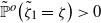 $\tilde{\mathbb{P}}^o\big(\tilde{\zeta}_1=\zeta\big)>0$
by irreducibility, it follows from the assumption that
 \begin{equation}\begin{aligned}\tilde{\mathbb{P}}^A\left(\tilde{\tau}_{o}=\infty\right)=0.\end{aligned}\end{equation}
When  $o\in\bar{A}$
, let
 $A_{\rm odd}=A\cap\mathbb{T}_i$
for some i with an odd number of vertices; by (6.6) and (6.7),
 \begin{equation}\begin{aligned}\tilde{\mathbb{P}}^{\zeta_A}\left(\tilde{\tau}_{o}=\infty\right)\le \tilde{\mathbb{P}}^{\zeta_{A_{odd}}}\left(\tilde{\tau}_{o}=\infty\right)=0 .\end{aligned}\end{equation}
Thus, from (6.7) and (6.8), we can get (6.5).
But if the claim (6.5) is true,
 \begin{equation*}\tilde{\mathbb{P}}^o\big(o\in\tilde{\zeta}^{\mathbb{T}_d}_t\text{ i.o.}\big)=1,\end{equation*}
which is impossible by Lemma 7, so that the assumption is false.
Next, when  $\beta\left(d\right)>\frac{1}{\sqrt{d}\,}$
, we will use the method of proving [Reference Handjani9, Lemma 2.2] to get the result. By the assumption,
 \begin{equation}\begin{aligned}\lim\limits_{k\to\infty}\lim\limits_{t\to\infty}\tilde{\mathbb{P}}^o\left({\rm diam}\big(\big[\tilde{\zeta}^{\mathbb{T}_d}_t\big]\big)\ge k\right)= 0.\end{aligned}\end{equation}
Since  $\tilde{\zeta}^{\mathbb{T}_d}_t$
is not positive recurrent,
 \begin{equation}\begin{aligned}\lim\limits_{k\to\infty}\lim\limits_{t\to\infty}\tilde{\mathbb{P}}^o\left(\tilde{\zeta}^{\mathbb{T}_d}_t\subseteq B_k\left(o\right)\right)= 0.\end{aligned}\end{equation}
Then, it follows from (6.9) and (6.10) that
 \begin{align*}\lim\limits_{t\to\infty}\tilde{\mathbb{P}}^o\left(o\in\tilde{\zeta}^{\mathbb{T}_d}_t\right)& \le \lim\limits_{k\to\infty}\lim\limits_{t\to\infty}\tilde{\mathbb{P}}^o\left(\tilde{\zeta}^{\mathbb{T}_d}_t\subseteq B_k\left(o\right)\right)+\lim\limits_{k\to\infty}\lim\limits_{t\to\infty}\tilde{\mathbb{P}}^o\left({\rm diam}\big(\big[\tilde{\zeta}^{\mathbb{T}_d}_t\big]\big)\ge k\right)\\&= 0,\end{align*}
which is impossible by Remark 4 and Lemma 3, so the assumption is again false. Thus, we have proved that  $\big[\tilde{\zeta}^{\mathbb{T}_d}_t\big]$
is not positive recurrent for any d satisfying
 $\beta\left(d\right)\ne\frac{1}{\sqrt{d}\,}$
.
Lemma 9. If  $\beta\left(d\right)\ne\frac{1}{\sqrt{d}\,}$
, for any
 $k>0$
and finite A,
 \begin{equation*}\tilde{\mathbb{P}}^{\zeta_A}\left(|\tilde{\zeta}^{\mathbb{T}_d}_t|=k \mid \tilde\zeta_t^{\mathbb{T}_d}\ne\textbf{0},\text{ for all}\ t\right)\to 0.\end{equation*}
Proof. For  $k=1$
, by Lemma 8 the process is not positive recurrent, so that
 \begin{equation*}\tilde{\mathbb{P}}^{\zeta_A}\left(|\tilde{\zeta}^{\mathbb{T}_d}_t|=1 \mid \tilde\zeta_t^{\mathbb{T}_d}\ne\textbf{0},\text{ for all}\ t\right)=\tilde{\mathbb{P}}^{\zeta_A}\left(\tilde{\zeta}^{\mathbb{T}_d}_t=\left[\left\{o\right\}\right] \mid \tilde\zeta_t^{\mathbb{T}_d}\ne\textbf{0},\text{ for all}\ t\right)\to 0.\end{equation*}
For  $k\ge 2$
, it is easy to verify that [Reference Handjani9, Proposition 2.6] also holds for the threshold-one voter model on
 $\mathbb{T}_d$
.
Since  ${\zeta}^{\mathbb{T}_d}_t$
has no independent death rate, the method of the proofs of Propositions 1 and 2 is no longer applicable. However, inspired by [Reference Handjani9, Proposition 3.2], we can still prove the following proposition when
 $\beta\left(d\right)\ne\frac{1}{\sqrt{d}\,}$
.
Proposition 3. If  $\beta\left(d\right)\ne\frac{1}{\sqrt{d}}$
, for any translation-invariant distribution
 $\mu$
satisfying
 $\mu\left(\zeta=\textbf{0}\text{ or }\textbf{1}\right)=0$
or
 $\mu=\delta_\zeta$
, where
 $\zeta$
is doubly dense as defined in (2.3), we have
 $\lim_{t\to\infty}\delta_{\zeta} U(t)= \mu_{1/2}^d$
, where U(t) is the Markov semigroup of
 ${\zeta}^{\mathbb{T}_d}_t$
and
 $\mu_{1/2}^d$
is the limiting distribution of the product measure with parameter 1/2.
Proof. Let  $\Omega_{\infty}=\big\{\tilde{\zeta}^{\mathbb{T}_d}_t\ne\textbf{0}\text{ for all}\ t \big\}$
. By annihilating duality (3.3), it suffices to prove that
 \begin{equation*}\mathbb{P}^{\mu,\zeta_A}\left( \zeta_{2}^{\mathbb{T}_d}\cap\tilde{\zeta}^{\mathbb{T}_d}_t\text{ is odd }\right)\to\frac{1}{2}\tilde{\mathbb{P}}^{\zeta_A}\left(\Omega_\infty\right)\end{equation*}
when  $\mathbb{\tilde{P}}^{\zeta_A}\left(\Omega_\infty\right)>0$
. Note that by the transition rates of
 $\tilde{\zeta}^{\zeta_A,\mathbb{T}_d}_t$
,
 $\big|\tilde{\zeta}^{\zeta_A,\mathbb{T}_d}_t\big|$
is always odd when
 $|A|$
is odd, so that
 $\mathbb{\tilde{P}}^{\zeta_A}\left(\Omega_\infty\right)=1$
when
 $|A|$
is odd.
Define  $\bar{\zeta}^{\mathbb{T}_d}_1=\big\{x\in \mathbb{T}_d\,{:}\,\zeta^{\mathbb{T}_d}_1\left(x\right)=1, \zeta^{\mathbb{T}_d}_1(\overleftarrow{x})=0\text{ or }\zeta^{\mathbb{T}_d}_1\left(x\right)=0, \zeta^{\mathbb{T}_d}_1(\overleftarrow{x})=1\big\}$
, where
 $\overleftarrow{x}$
is the the parent of x. Since
 $\big|\tilde{\zeta}_t^{\mathbb{T}_d}\big|\to\infty$
in probability on
 $\Omega_{\infty}$
by Lemma 9, applying the proof of (4.20) in Proposition 1, in order to prove that
 $\big|\bar{\zeta}_1^{\mathbb{T}_d}\cap\tilde{\zeta}_t^{\mathbb{T}_d}\big|\to\infty$
in probability under
 $\mathbb{P}^{\mu,\zeta_A}$
on
 $\Omega_{\infty}$
, we only need to show that when
 $\mu=\delta_\zeta$
for some doubly dense configuration
 $\zeta$
, we have
 $\inf\limits_x\mathbb{P}^\zeta\big(\bar\zeta_1^{\mathbb{T}_d}\left(x\right)=1\big)>0$
.
Let  $\mathcal{I}_x=\left\{\eta\,{:}\,\text{there exist } y, z \in B_N\left(x\right),\zeta\left(y\right)=0,\zeta\left(z\right)=1\right\}$
. Then
 \begin{equation*}\begin{aligned} \inf\limits_x\mathbb{P}^\zeta\left(\bar\zeta_1^{\mathbb{T}_d}\left(x\right)=1\right) &\geq\inf\limits_{x}\inf\limits_{\zeta\in\mathcal{I}_x}\mathbb{P}^\zeta\left(\bar\zeta_1^{\mathbb{T}_d}\left(x\right)=1\right) \\[2pt] &=\inf\limits_{\zeta\in\mathcal{I}_o}\mathbb{P}^\zeta\left(\bar\zeta_1^{\mathbb{T}_d}\left(o\right)=1\right)\qquad\qquad\text{ by translation invariance} \\[2pt] &=\inf\limits_{\zeta\in\mathcal{I}_o}\mathbb{P}^{\zeta_{\left\{o,\overleftarrow{o}\right\}}}\left(\tilde{\zeta}^{\mathbb{T}_d}_1\cap\zeta\text{ is odd}\right)\quad\text{by duality} \\[2pt] &\geq \inf\limits_{\zeta\in\mathcal{I}_o}\mathbb{P}^{\zeta_{\left\{o,\overleftarrow{o}\right\}}}\left(\tilde{\zeta}^{\mathbb{T}_d}_1\subset B_N\left(o\right)\text{ and }\tilde{\zeta}^{\mathbb{T}_d}_1 \cap\zeta\text{ is odd}\right)\\[2pt] &=\inf\limits_{\zeta\subseteq B_N\left(o\right),\zeta\in\mathcal{I}_o}\mathbb{P}^{\zeta_{\left\{o,\overleftarrow{o}\right\}}}\left(\tilde{\zeta}^{\mathbb{T}_d}_1\subseteq B_N\left(o\right),\tilde{\zeta}^{\mathbb{T}_d}_1 \cap\zeta\text{ is odd}\right)\\[2pt] &=p>0,\end{aligned}\end{equation*}
where the last equality holds because that there are finite configurations satisfying  $\zeta\subseteq B_N\left(o\right)$
and each has a subset of an odd number of vertices.
Let 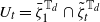 $U_t=\bar{\zeta}_1^{\mathbb{T}_d}\cap\tilde{\zeta}_t^{\mathbb{T}_d}$
and
 $V_t=\left\{x\,{:}\,x\in U_t, \text{ \textit{x} is isolated}\right\}$
, where x is isolated if and only if
 $T_n^{y,S_y}\cap [1,2]=\emptyset$
when
 $S_y\cap\left\{x,\overleftarrow{x}\right\}\ne\emptyset$
, or
 $\left(y,S_y\right)=\left(x,S_x\right)$
for some
 $S_x$
, or
 $\left(y,S_y\right)=\left( \overleftarrow{x},S_{\overleftarrow{x}}\right)$
for some
 $S_{\overleftarrow{x}}\ne\left\{x\right\}$
. This ensures that
•
$\text{for all}\ x\in V_t $
, if
${\zeta}^{\mathbb{T}_d}_1\left(x\right)=1$
then
$\zeta^{\mathbb{T}_d}_2\left(x\right)=1$
if and only if there is no arrow from
$\overleftarrow{x}$
to x at [1, 2];•
$\text{for all}\ x\in V_t $
, if
${\zeta}^{\mathbb{T}_d}_1\left(x\right)=0$
then
$\zeta^{\mathbb{T}_d}_2\left(x\right)=1$
if and only if there is at least an arrow from
$\overleftarrow{x}$
to x at [1, 2].


It follows that
 \begin{equation}\begin{aligned}|\bar{\zeta}_{2}^{\mathbb{T}_d}\cap\tilde{\zeta}^{\mathbb{T}_d}_t\cap V_t|=&\sum\limits_{x\in V_t,\zeta_1^{\mathbb{T}_d}\left(x\right)=1}\textrm{1}_{\left\{\text{there is no arrow from} \overleftarrow{x}\text{ to \textit{x} at [1,2]}\right\}}\\[3pt] &+\sum\limits_{x\in V_t,\zeta_1^{\mathbb{T}_d}\left(x\right)=0}\textrm{1}_{\left\{\text{there is at least an arrow from} \overleftarrow{x}\text{ to \textit{x} at [1,2]}\right\}}.\end{aligned}\end{equation}
Let
 \begin{align} g_x & = \textrm{1}_{\left\{{\zeta}^{\mathbb{T}_d}_1\left(x\right)=1,\text{ there is no arrow from} \overleftarrow{x}\text{ to \textit{x} at [1,2]}\right\}} \nonumber \\[3pt] & \quad + \textrm{1}_{\left\{{\zeta}^{\mathbb{T}_d}_1\left(x\right)=0,\text{ there is at least an arrow from } \overleftarrow{x}\text{ to \textit{x} at [1,2]}\right\}}, \nonumber \\[3pt] h & = 1-\left\{|\bar{\zeta}_{2}^{\mathbb{T}_d}\cap\tilde{\zeta}^{\mathbb{T}_d}_t\cap V^c_t| \text{ mod 2}\right\}, \\[3pt] \mathcal{G}_t & = \sigma\big(V_t,h,\zeta_1^{\mathbb{T}_d}\big).\nonumber \end{align}
Note that  $\left\{x\in V_t\right\}_{x\in U_t}$
are 2-dependent, thus
 $|V_t|\to \infty$
in probability under
 $\mathbb{P}^{\mu,\zeta_A}$
on
 $\Omega_\infty$
. Since, given
 $ \mathcal{G}_t$
,
 $V_t$
,
 $\zeta_1^{\mathbb{T}_d}$
, and h are constant and
 $\left\{g_x, x\in V_t\right\}$
are mutually independent and independent of
 $ \mathcal{G}_t$
, by (6.11), (6.12), and [Reference Bramson, Ding and Durrett3, Lemma 2.3],
 \begin{align*}\left|\mathbb{P}^{\mu,\zeta_A}\left( \bar{\zeta}_{2}^{\mathbb{T}_d}\cap\tilde{\zeta}^{\mathbb{T}_d}_t\text{ is odd} \mid \mathcal{G}_t\right)-\frac{1}{2}\right|&=\left|\mathbb{P}^{\mu,\zeta_A}\left(\sum\limits_{x\in V_t}g_x=h \text{ mod 2} \mid \mathcal{G}_t\right)-\frac{1}{2}\right|\\&\leq\left(1-2{\rm e}^{-1}\right)^{|V_t|}\to 0\end{align*}
in probability on  $\Omega_{\infty}$
. Taking expectation, by the bounded convergence theorem,
 \begin{align*}\mathbb{P}^{\mu}\left( \zeta_{2+t}\cap\zeta_A\text{ is odd} \mid \Omega_{\infty}\right)=\mathbb{P}^{\mu,\zeta_A}\big( \zeta_{2}^{\mathbb{T}_d}\cap\tilde{\zeta}^{\mathbb{T}_d}_t\text{ is odd} \mid \Omega_{\infty}\big)\to\frac{1}{2}. \end{align*}
Inspired by the proof of [Reference Handjani9, Proposition 3.5], we will use a comparison of  $\zeta^{\mathbb{T}_d}_{t}$
and
 $\eta^{\varepsilon,\mathbb{T}_d}_{t}$
for some
 $\delta>0$
to prove the complete convergence theorem for
 $\zeta^{\mathbb{T}_d}_{t}$
when it survives strongly.
Proof of Theorem 7. When  $\beta\left(d\right)<\frac{1}{\sqrt{d}\,}$
, the result follows from Proposition 3, so that we only need to prove the result when
 $\zeta^{\mathbb{T}_d}_{t}$
survives strongly. Since 0 and 1 are equivalent, we may as well assume that
 $\sum_{x}\left[1-\zeta\left(x\right)\right]=\infty$
. Then it suffices to prove that, for any finite
 $B,\zeta\ne\textbf{0}$
,
 \begin{equation*}\mathbb{P}^\zeta\big(\zeta^{\mathbb{T}_d}_{t}\cap B\text{ is odd} \mid \tau_{\textbf{0}}=\infty\big)\to\frac{1}{2}\mu\left(\zeta\,{:}\,\zeta\cap\zeta_B\text{ is odd}\right)=\frac{1}{2}\tilde{\mathbb{P}}^{\zeta_B}\left(\Omega_{\infty} \right)\end{equation*}
when  $\tilde{\mathbb{P}}^{\zeta_B}\left(\Omega_{\infty} \right)>0$
.
From the argument of [Reference Liggett14, Theorem 4.65(c)], we can prove that  $\eta^{\varepsilon,\mathbb{T}_d}_t$
does not survive strongly when
 $\varepsilon=\varepsilon_2\left(d\right)$
. It follows that
 $\varepsilon_2\left(d\right)>0$
, therefore there exists
 $\varepsilon>0$
such that
 $\eta^{\varepsilon,\mathbb{T}_d}_t$
survives strongly, so that we have the domination
 $\eta^{\varepsilon,\mathbb{T}_d}_t\le\zeta^{\mathbb{T}_d}_{t}\le\hat{\zeta}^{\varepsilon,\mathbb{T}_d}_t$
, where
 $\hat{\zeta}^{\varepsilon,\mathbb{T}_d}_t$
denotes the threshold-one voter model with spontaneous birth rate
 $\varepsilon$
. By Lemma 6 and Remark 4, for any
 $\epsilon>0$
, choose N such that, for any finite subset D satisfying
 $|D|\geq N$
,
 \begin{equation}\begin{aligned}&\mathbb{P}^{\zeta_D}\big(\zeta^{\mathbb{T}_d}_t\ne\emptyset \text{ for all\ t}\big)>1-\epsilon ,\\&\mathbb{P}^{\zeta_D}\big(\eta^{\varepsilon,\mathbb{T}_d}_t\ne\emptyset \text{ for all\ t}\big)>1-\epsilon.\end{aligned}\end{equation}
It is easy to verify that  $|\zeta^{\mathbb{T}_d}_t|\to\infty$
a.s. on
 $\left\{\tau_{\textbf{0}}=\infty\right\}$
, thus we can choose U such that
 \begin{equation}\begin{aligned}\mathbb{P}^{\zeta}\big(|\zeta^{\mathbb{T}_d}_t|\geq N \mid \tau_{\textbf{0}}=\infty\big)>1-\epsilon\end{aligned}\end{equation}
for any  $t\geq U$
.
By Theorem 5, there exist translation-invariant measures  $\nu_a$
and
 $\nu_b$
such that
 \begin{equation}\begin{aligned}&\delta_{\zeta_D}S^{\varepsilon}\left(t\right)\to\epsilon'\nu_b+\left[1-\epsilon'\right] \delta_{\textbf{0}},\\&\delta_{\zeta_D}\hat S^{\varepsilon}\left(t\right)\to \nu_a,\end{aligned}\end{equation}
where  $\epsilon'=\mathbb{P}^{\zeta_D}\big(\eta^{\varepsilon,\mathbb{T}_d}_t \text{ dies out}\big)<\epsilon$
.
Let
 \begin{equation}\begin{aligned}\tilde{\nu}_b=\epsilon\delta_0+\left(1-\epsilon\right)\nu_b.\end{aligned}\end{equation}
By Proposition 3,
 \begin{equation*}\tilde{\nu}_bU\left(t\right)\to\epsilon\delta_0+\left(1-\epsilon\right)\mu_{1/2}^d, \qquad \nu_aU\left(t\right)\to\mu_{1/2}^d.\end{equation*}
Observe that
 \begin{equation*}\textrm{1}_{\left\{\zeta^{\mathbb{T}_d}_t\cap B\text{ is odd}\right\}}=\frac{1}{2}\bigg[1-\prod_{x\in B}\bigg[1-2\zeta^{\mathbb{T}_d}_t\left(x\right)\bigg]\bigg],\end{equation*}
which is a linear combination of at most  $2^{|B|}$
increasing functions of the form
 \begin{equation*}\prod_{x\in C}\zeta^{\mathbb{T}_d}_t\left(x\right), \qquad C\subseteq B,\end{equation*}
so that, for any sufficient large T,
 \begin{equation*}\big|\mathbb{P}^{\rho}\big(\zeta^{\mathbb{T}_d}_T\cap B\text{ is odd }\big)-\frac{1}{2}\tilde{\mathbb{P}}^{\zeta_B}\left(\Omega_{\infty} \right)\big|<2^{|B|+1}\epsilon\end{equation*}
uniformly for any  $\tilde{\nu}_b\le\rho\leq\nu_a$
.
Then, for any D satisfying  $|D|\ge N$
, and for any sequence
 $\left\{ t_n\right\}$
, since the space of all probability measures is compact, there exists
 $\left\{r_n\right\}\subset\left\{t_n-T-U\right\}$
such that
 $\zeta_DS\left(r_n\right)\to\rho$
. Then, by (6.15) and (6.16),
 $\tilde{\nu}_b\leq\rho\leq\nu_a$
. It follows that
 \begin{align} \lim\limits_{n\to\infty}\left|\mathbb{P}^{\zeta_D}\big(\zeta^{\mathbb{T}_d}_{r_n+T}\cap B\text{ is odd}\big)-\frac{1}{2}\tilde{\mathbb{P}}^{\zeta_B}\left(\Omega_{\infty} \right)\right|&= \left|\mathbb{P}^{\rho}\big(\zeta^{\mathbb{T}_d}_T\cap B\text{ is odd}\big)-\frac{1}{2}\tilde{\mathbb{P}}^{\zeta_B}\left(\Omega_{\infty} \right)\right|\nonumber\\&<2^{|B|+1}\epsilon.\end{align}
 \begin{equation} \limsup\limits_{n\to\infty}\left|\mathbb{P}^{\zeta_D}\left(\zeta^{\mathbb{T}_d}_{r_n+T}\cap B\text{ is odd} \mid \tau_{\textbf{0}}=\infty\right)-\frac{1}{2}\tilde{\mathbb{P}}^{\zeta_B}\left(\Omega_{\infty} \right)\right|<2^{|B|+2}\epsilon. \end{equation}
 \begin{equation*}\limsup\limits_{n\to\infty}\left|\mathbb{P}^\zeta\left(\zeta^{\mathbb{T}_d}_{r_n+T+U}\cap B\text{ is odd} \mid \tau_{\textbf{0}}=\infty\right)-\frac{1}{2}\tilde{\mathbb{P}}^{\zeta_B}\left(\Omega_{\infty} \right)\right|<2^{|B|+3}\epsilon.\end{equation*}
Then we can get the desired result by letting  $\epsilon\to 0$
.
Appendix A. Proof of Theorem 3
Recall the definition
 \begin{equation}\begin{aligned} f\left(A\right)=\lim\limits_{\epsilon\to 0}\frac{1-\nu_{\epsilon}(\eta=0 \text{ on \textit{A})}}{\nu_{\epsilon}\left(\eta\left(x\right)=1\right)} ,\end{aligned}\end{equation}
where  $\nu_{\epsilon}$
is the translation-invariant measure on
 $\mathbb{T}_2$
satisfying the following conditions:
•
$\nu_{\epsilon}\left(\eta\left(x\right)=1\right)=\frac{\epsilon}{q+\epsilon}$
;•
$\nu_{\epsilon}\left(\eta\left(x\right)=0 \mid \eta\left(y\right)=1\right)=q$
,
$\nu_{\epsilon}\left(\eta\left(x\right)=0 \mid \eta\left(y\right)=0\right)=1-\epsilon$
when
$x\sim y$
;• conditional on
$\eta\left(x\right)$
,
$\eta(x_{\left(1\right)})$
,
$\eta(x_{(2)})$
,
$\eta(x_{(3)})$
are independent with respect to
$\nu_{\epsilon}$
, where
$x_{\left(i\right)}$
,
$1\le i\le 3$
, are the neighbors of x.




One may explicitly construct such a measure by defining a 0–1 random variable on o according to its marginal and then recursively define them on  $\partial B_n\left(o\right)$
in each step.
The existence of  $f\left(A\right)$
is easy to prove. For finite and nonempty A, denote by
 $y_{A}$
a site in A with the minimum generation. For a configuration
 $\psi\in \left\{0,1\right\}^A$
, define the subset
 $D_{\psi}=\left\{y\,{:}\,\psi\left(y\right)=1\right\}$
.
Note that  $\tilde{\xi}^{\lambda,\mathbb{T}_d}_t$
is the Markov process on the countable space Y now, where Y is the set of all finite subsets of
 $\mathbb{T}_d$
, thus the derivation of
 $\mathbb{E}^{\xi_A}f\left(\tilde{\xi}^{\lambda,\mathbb{T}_d}_t\right)$
is applicable even though f is discontinuous in
 $\left\{0,1\right\}^{\mathbb{T}_d}$
on the ordinary topology.
Denote by  $\mathcal{B}$
the set of the components of A; then
 \begin{equation}\begin{aligned} h\left(A\right)&=\frac{{\rm d}}{{\rm d} t}\mathbb{E}^{\xi_A}f\left(\tilde{\xi}^{\lambda,\mathbb{T}_d}_t\right)\Big|_{t=0} \\&=\sum\limits_{B}q\left(A,B\right)\left[\,f\left(B\right)-f\left(A\right)\right] \\&=\lambda\sum\limits_{x\in A}\lim\limits_{\epsilon\to 0}\frac{\nu_{\epsilon}\left(\eta=0 \text{ on \textit{A}}, \text{there exists } x*\sim x \text{ such that } \eta\left(x*\right)=1\right)}{\nu_{\epsilon}\left(\eta\left(x\right)=1\right)}\\& \quad -\sum\limits_{x\in A}\nu\left(\eta=0 \text{ on \textit{A}}\backslash\left\{x\right\} \mid \eta\left(x\right)=1\right) \\&=\sum\limits_{B\in\mathcal{B}}\sum\limits_{x\in B}\bigg[\lambda\!\!\sum\limits_{\psi\in\left\{0,1\right\}^{\mathcal{N}_x}, D_{\psi}\ne\emptyset}\!\!\!\!\!\!\nu\left(\eta=0 \text{ on } A,\eta=\psi \text{ on }\mathcal{N}_x \mid \eta\left(y_{D_\psi}\right)=1\right)\bigg]\\& \quad \times \sum\limits_{x\in A}\nu\left(\eta=0 \text{ on A}\backslash\left\{x\right\} \mid \eta\left(x\right)=1\right)\\&\overset{\vartriangle}{=} \sum\limits_{B\in\mathcal{B}}h_B\left(A\right)- \sum\limits_{x\in A}\nu\left(\eta=0 \text{ on A}\backslash\left\{x\right\} \mid \eta\left(x\right)=1\right) , \end{aligned}\end{equation}
where  $h_B\left(A\right)$
can be seen as the contributions of B.
Next, we want to show that (A.2) has the same form as [Reference Liggett13, (4.2)]. Since there is not much difference in the case when  $|B|=1$
or
 $|B|>1$
, we just prove the case
 $|B|=1$
and the other case follows from the same strategy.
When  $B=\left\{x\right\}$
is a singleton,
 $\mathcal{N}_x\cap A=\left\{x\right\}$
. Define
 \begin{align*}\gamma\left(y\right)=1-\nu\left(\eta=0\text{ on } A\cap S_y\left(x\right) \mid \eta\left(y\right)=1\right)\!,\end{align*}
where  $S_y\left(x\right)$
is the connected component of
 $\mathbb{T}_d\backslash\left\{x\right\}$
containing y. Then
 \begin{align*} h_B\left(A\right)&=\lambda\big[\nu\left(\eta=0 \text{ on }A,\eta\left(x_{\left(1\right)}\right)=1,\eta\left(x_{(2)}\right)=0,\eta\left(x_{(3)}\right)=0 \mid \eta\left(x_{\left(1\right)}\right)=1\right)\\[2pt]&\quad +\nu\left(\eta=0 \text{ on } A,\eta\left(x_{\left(1\right)}\right)=1,\eta\left(x_{(2)}\right)=1,\eta\left(x_{(3)}\right)=0 \mid \eta\left(x_{\left(1\right)}\right)=1\right)\\[2pt] &\quad +\nu\left(\eta=0 \text{ on }A,\eta\left(x_{\left(1\right)}\right)=1,\eta\left(x_{(2)}\right)=1,\eta\left(x_{(3)}\right)=1 \mid \eta\left(x_{\left(1\right)}\right)=1\right)\\[2pt] &\quad +\nu\left(\eta=0 \text{ on }A,\eta\left(x_{\left(1\right)}\right)=1,\eta\left(x_{(2)}\right)=0,\eta\left(x_{(3)}\right)=1 \mid \eta\left(x_{\left(1\right)}\right)=1\right)\displaybreak\\ &\quad +\nu\left(\eta=0 \text{ on }A,\eta\left(x_{\left(1\right)}\right)=0,\eta\left(x_{(2)}\right)=1,\eta\left(x_{(3)}\right)=0 \mid \eta\left(x_{(2)}\right)=1\right)\\[2pt] &\quad +\nu\left(\eta=0 \text{ on }A,\eta\left(x_{\left(1\right)}\right)=0,\eta\left(x_{(2)}\right)=1,\eta\left(x_{(3)}\right)=1 \mid \eta\left(x_{(2)}\right)=1\right)\\[2pt] &\quad +\nu\left(\eta=0 \text{ on }A,\eta\left(x_{\left(1\right)}\right)=0,\eta\left(x_{(2)}\right)=0,\eta\left(x_{(3)}\right)=1 \mid \eta\left(x_{(3)}\right)=1\right)\big]\\[2pt] &\quad \overset{\vartriangle}{=}\lambda\times\left[\left(1\right)+(2)+(3)+(4)+(5)+(6)+(7)\right].\end{align*}
Since the proofs for (1), (5), and (7) are similar, we just take (1) as an example:
 \begin{align*}&\nu\left(\eta=0 \text{ on A},\eta\left(x_{\left(1\right)}\right)=1,\eta\left(x_{(2)}\right)=0,\eta\left(x_{(3)}\right)=0 \mid \eta\left(x_{\left(1\right)}\right)=1\right)\\[3pt] &=\nu\left(\eta=0 \text{ on A}\cap\left[ \mathbb{T}_2\backslash S_{x_{\left(1\right)}}\left(x\right)\right],\eta\left(x_{(2)}\right)=0,\eta\left(x_{(3)}\right)=0 \mid \eta\left(x\right)=0\right)\\[3pt] &\quad\times\nu\left(\eta\left(x\right)=0\mid\eta\left(x_{\left(1\right)}\right)=1\right)\nu\left(\eta=0 \text{ on A}\cap S_{x_{\left(1\right)}}\left(x\right)\mid\eta\left(x_{\left(1\right)}\right)=1\right) \\[3pt] &=q\nu\left(\eta=0 \text{ on A}\cap S_{x_{\left(1\right)}}\left(x\right)\mid \eta\left(x_{\left(1\right)}\right)=1\right)\\[3pt] &=q\left(1-\gamma\left(x_{\left(1\right)}\right)\right). \end{align*}
Similarly, we take (2) as an example to prove that (2), (3), (4), and (6) all equal 0:
 \begin{align*}&\nu(\eta=0 \text{ on A},\eta(x_{(1)})=1),\eta(x_{(2)})=1,\eta(x_{(3)})=0\mid\eta(x_{(1)})=1)\\[3pt] &=\nu(\eta=0 \text{ on A}\cap( T_2\backslash S_{x_{(1)}}(x)),\eta(x_{(2)})=1,\eta(x_{(3)})=0\mid\eta(x)=0)\\[3pt] &\quad\times\nu(\eta(x)=0\mid\eta(x_{(1)})=1)\nu(\eta=0 \text{ on A}\cap S_{x_{(1)}}(x)\mid\eta(x_{(1)})=1) \\[3pt] &\leq \nu(\eta(x_{(2)})=1\mid\eta(x)=0)\\[3pt] &=0. \end{align*}
Thus,
 \begin{equation*}\begin{aligned} h_B\left(A\right)=\lambda q\sum\limits_{i=1}^{3}\left[1-\gamma\left(x_{\left(i\right)}\right)\right]-\prod_{i=1}^{3}\left[1-\left(1-q\right)\gamma\left(x_{\left(i\right)}\right)\right],\end{aligned}\end{equation*}
which is the same as [Reference Liggett13, (4.2)], such that
 \begin{equation*}\begin{aligned} h\left(A\right)= \lambda\sum\limits_{x\in A,y\not\in A,x\sim y}\nu\left(\eta=0 \text{ on }A\mid\eta\left(y\right)=1\right)-\sum\limits_{x\in A}\nu\left(\eta= 0 \text{ on } A\mid\eta\left(x\right)=1\right) ,\end{aligned}\end{equation*}
so that, by the argument on [Reference Liggett13, pp. 1693, 1695],  $h\left(A\right)\geq 0$
when
 $\lambda\geq 0.6369$
. Specifically,
 \begin{equation}\begin{aligned} \sum\limits_{x\in A,y\not\in A,x\sim y}\nu\left(\eta=0 \text{ on }A\mid\eta\left(y\right)=1\right)\geq\frac{1}{0.6369}\sum\limits_{x\in A}\nu\left(\eta= 0 \text{ on } A\mid\eta\left(x\right)=1\right).\end{aligned}\end{equation}
Next, we want to get a nonnegative supermartingale. First we have the following lemma:
Lemma 10. (Page 1690 of [Reference Liggett13].) Suppose that  $\xi_t$
is a pure jump process on a countable set with transition rates
 $q\left(A,B\right)$
, and that f satisfies the following conditions for some
 $0<C, M<\infty$
:
(i)
$ \text{for all}\ A,\ \sum\limits_B q\left(A,B\right)\left[\,f\left(B\right)-f\left(A\right)\right]\geq Cf\left(A\right)$
;(ii)
$|f\left(B\right)-f\left(A\right)|\leq M$
whenever
$q\left(A,B\right)>0$
;(iii)
$q\left(A\right)\leq Cf\left(A\right),\text{ for all}\ A$
.




Then,  $f\left(\xi_{t\land\tau}\right)^{-1}$
is a supermartingale where
 $\tau=\inf\left\{t,f\left(\xi_t\right)\le c\right\}$
for some sufficiently large c.
Now we only need to show that the test function (A.1) satisfies the conditions in Lemma 10. For any  $x\in A$
,
 \begin{equation}\begin{aligned}1&\geq f\left(A\right)-f\left(A\backslash\left\{x\right\}\right)\\[3pt] &=\prod_{x_{\left(i\right)}}\nu\left(\eta=0 \text{ on }A\cap S_{x_{\left(i\right)}}\left(x\right)\mid\eta\left(x\right)=1\right)\\[3pt] &\ge\prod_{x_{\left(i\right)}}\nu\left(\eta=0 \text{ on }A\cap S_{x_{\left(i\right)}}\left(x\right),\eta\left(x\left(i\right)\right)=0\mid\eta\left(x\right)=1\right)\\[3pt] &= q^3.\end{aligned}\end{equation}
For any  $x\in A$
satisfying
 $\mathcal{N}_x\cap A\ne\emptyset$
, assume
 $x_{\left(1\right)}\not\in A$
; by (A.4),
 \begin{equation}\begin{aligned}7\geq f\left(A\cup\mathcal{N}_x\right)-f\left(A\right)&=\!\!\!\!\sum\limits_{\psi\in\left\{0,1\right\}^{\mathcal{N}_x}, D_{\psi}\ne\emptyset}\!\!\!\!\!\!\!\!\!\!\!\!\nu\left(\eta=0 \text{ on } A,\eta=\psi \text{ on }\mathcal{N}_x \mid \eta\left(y_{D_\psi}\right)=1\right)\\[3pt] &\geq\nu\left(\eta=0\text{ on }A\cup\left\{x_{(2)},x_{(3)}\right\}\mid\eta\left(x_{\left(1\right)}\right)=1\right)\\[3pt] &\geq q^3.\end{aligned}\end{equation}
It follows that
 \begin{equation}\begin{aligned} C_1|A|\leq f\left(A\right)\leq C_2|A|.\end{aligned}\end{equation}
When  $\lambda>0.6369$
,
 \begin{equation}\begin{aligned}&\sum\limits_B q\left(A,B\right)\left[\,f\left(B\right)-f\left(A\right)\right]\\&=\left(\lambda-0.6369\right)\sum\limits_{x\in A,y\not\in A,x\sim y}\nu\left(\eta=0 \text{ on }A\mid\eta\left(y\right)=1\right)\\&+\left[0.6369\!\!\!\!\!\!\sum\limits_{x\in A,y\not\in A,x\sim y}\!\!\!\!\!\!\nu\left(\eta=0 \text{ on }A\mid\eta\left(y\right)=1\right)-\sum\limits_{x\in A}\nu\left(\eta=0\text{ on } A\backslash\left\{x\right\}\mid\eta\left(x\right)=1\right)\right]\\&\geq\frac{\lambda-0.6369}{0.6369}\sum\limits_{x\in A}\nu\left(\eta=0\text{ on } A\backslash\left\{x\right\}\mid\eta\left(x\right)=1\right) \qquad \text{by (\linkref{eqn67}{A.3})}\\&\geq C_3|A|\qquad \text{by (\linkref{eqn68}{A.4})}\\&\geq C_4f\left(A\right) \qquad \text{by (\linkref{eqn70}{A.6})}.\end{aligned}\end{equation}
When  $q\left(A,B\right)>0$
, by (A.5) and (A.4),
 \begin{equation}\begin{aligned}|f\left(A\right)-f\left(B\right)|\leq 7,\end{aligned}\end{equation}
and since  $q\left(A\right)\leq C_5|A|$
, it follows from (A.6) that
 \begin{equation}\begin{aligned} q\left(A\right) \leq C_6f\left(A\right),\end{aligned}\end{equation}
where  $C_i$
,
 $1\leq i\leq 6$
, are positive and finite constants. Then, (A.7), (A.8), and (A.9) give that
 $\tilde{\xi}^{\lambda,A,\mathbb{T}_d}_t$
satisfies the conditions of Lemma 10, and thus
 $f\left(\xi^{\lambda,A,\mathbb{T}_d}_{t\land\tau}\right)^{-1}$
is a nonnegative supermartingale. By the argument in Section 4.2, the proof is complete.
 $\hfill\square$
Appendix B. Proof of Lemma 3
In order to prove Lemma 3, we need the following lemma, which can be proved easily by the strong Markov property (we omit the proof here).
Lemma 11. For any  $\lambda,d$
,
 \begin{equation}\begin{aligned}\lim\limits_{n\to\infty}\left[\sup\limits_t \mathbb{P}^o\left(x_n\in\xi^{\lambda,\hat{\mathbb{T}}^d_{x_n}}_t\right)\right]^{1/n}=\beta\left(\lambda,d\right).\end{aligned}\end{equation}
Proof of Lemma 3. By (B.1), for all a satisfying  $ \frac{1}{\sqrt{d}\,}<a<\beta\left(\lambda,d\right)$
, with n large enough, there exists t such that
 \begin{equation*}\begin{aligned} \mathbb{P}^o\left(x_n\in\xi^{\lambda,\hat{\mathbb{T}}^d_{x_n}}_t\right)> a^n.\end{aligned}\end{equation*}
Let  $B_0=\left\{o\right\}$
,
 $B_i=\cup_{x\in B_{i-1}}\big\{y\in \xi_t^{\lambda,\mathbb{T}^d_x},|y-x|=n\big\}$
, where
 $\xi^{\lambda,\mathbb{T}^d_x}_{\cdot}$
are independent copies of
 $\xi^{\lambda,\mathbb{T}^d_o}_\cdot$
. Then
 $|B_j|$
is a supercritical branching process since
 $\mathbb{E}|B_1|>\left(ad\right)^n>1$
by the domination of
 $\xi^{\lambda,\mathbb{T}^d_o}_{jt}$
. Let
 \begin{equation*}b=\left[\mathbb{P}^o\left(x_n\in\xi^{\lambda,\hat{\mathbb{T}}^d_{x_n}}_t\right)\right]^{1/n}\geq a;\end{equation*}
by the limit theorem for supercritical branching processes,  $\lim\limits_{j\to\infty}\frac{|B_j|}{\left(d^nb^n\right)^j}=X$
exists a.s. Thus, by [Reference Durrett6, Theorem 5.3.10],
 $X\not\equiv 0$
so that there exists
 $\epsilon>0$
such that
 \begin{equation}\begin{aligned} \mathbb{P}\left( |B_j|\geq\epsilon\left(da\right)^{nj}\right)\geq\epsilon\end{aligned}\end{equation}
for all sufficiently large j.
Now let  $r_i=\mathbb{P}^o\left(o\in\xi^{\lambda,\mathbb{T}_o^d}_{2ijt}\right)$
. Note that, by the strong Markov property,
 \begin{equation}\begin{aligned}\mathbb{P}^{x_{jn}}\left(o\in\xi^{\lambda,\mathbb{T}_o^d}_{jt}\right)\geq \left[\mathbb{P}^{o}\left(x_n\in\xi^{\lambda,\hat{\mathbb{T}}_{x_n}^d}_{t}\right)\right]^j\geq a^{nj}.\end{aligned}\end{equation}
By (B.3), the strong Markov property, and monotonicity,
 \begin{equation*}\begin{aligned}r_{i+1}&\geq \mathbb{P}^o\left(\text{there exists } |x|=jn, x\in\xi^{\lambda,\mathbb{T}_o^d}_{\left(2i+1\right)jt}\right)\mathbb{P}^{x_{jn}}\left(o\in\xi^{\lambda,\mathbb{T}_o^d}_{jt}\right)\\&\ge \mathbb{P}^o\left(\text{there exists } |x|=jn, x\in\xi^{\lambda,\mathbb{T}_o^d}_{\left(2i+1\right)jt}\right)a^{jn}\\&\geq\epsilon a^{jn}\left[1-\left(1-r_i\right)^{\lfloor\epsilon \left(ad\right)^{jn}\rfloor}\right]\qquad\text{ by (\linkref{eqn75}{B.2})}\\&\overset{\vartriangle}{=}f\left(r_i\right).\end{aligned}\end{equation*}
Note that f is an increasing function with  $f\left(0\right)=0$
,
 $f\left(1\right)=\epsilon a^{nj}<1$
,
 $f'\left(0\right)\geq\epsilon\lfloor\epsilon \left(a^2d\right)^{nj}\rfloor>1$
for some j sufficiently large. So, there exists
 $0<r^*<1$
such that
 $f\left(r^*\right)=r^*$
. Since
 $r_0=1>r^*$
, for any i we have
 $r_{i+1}\geq f\left(r_i\right)\geq f\left(r^*\right)=r^*$
. To extend to all times, simply use
 \begin{equation*}\mathbb{P}^o\left(o\in\xi^{\lambda,\mathbb{T}_d}_s\right)\geq {\rm e}^{-2jt}r_i, \qquad 2ijt\leq s
< 2\left(i+1\right)jt.\end{equation*}
Now the proof is complete.
Acknowledgements
The authors would like to thank Dr. Rick Durrett, Dr. Thomas Liggett, and Dr. Thomas Mountford for helpful comments.


