

1 Introduction
A majority of mandatory public pension systems in the world involve an earnings-related (ER) scheme with ‘pay-as-you-go’ financing. By earnings-related we refer to systems where the pension is essentially a function of past earnings. Three main designs can be identified: standard defined-benefit systems, points systems, and notional account systems; mathematically, the three benefit formulas are equivalent.Footnote 1 By pay-as-you-go we imply that pensions are financed essentially out of current contributions. Many of the systems can have reserves, but these act rather as a ‘buffer stock’ to smooth adjustments to benefits or contribution rates that become necessary as a result of unexpected macroeconomic and/or demographic shocks or the gradual maturation of the system.
Surprisingly, in most cases, ER systems do not meet basic principles in terms of design to ensure financial sustainability, minimize distortions in labor supply and savings decisions, and to avoid arbitrary – often regressive – redistributions of income. Even in countries that have recently adopted notional account schemes, which deal with issues related to incentives and equity, the problem of financial sustainability has not been fully resolved.
The focus of this paper is on this last problem: the financial sustainability of the scheme. It is well known that whether an ER system is financially self-sustainable or not depends on the implicit rate of return (IRR) that it pays on contributions. If the IRR is too high, the system becomes insolvent; if the IRR is too low the system penalizes workers. Until recently, it was common to refer to the growth rate of the covered wage bill as the appropriate measure of the IRR.Footnote 2 This is the correct measure, however, only in restrictive theoretical settings (e.g., two overlapping generation models in steady state). Reality is more complex and, while the growth rate of the covered wage bill can be a good proxy under some circumstances, other factors such as retirement patterns, mortality rates, and the age-sex composition of the plan members are important as well.
Settergren and Mikula (Reference Settergren2005) proposed a measure of the sustainable IRR that inspires the ‘automatic balancing mechanism’ in the current Swedish Notional Account pension system. It depends on the growth rate of the average wage, the growth rate of reserves, and the so called ‘turnover duration’ (TD) of the system. The TD is supposed to capture the average length of time that a monetary unit of contribution remains in the system. The authors argue that the TD multiplied by total contributions (the so-called contribution asset) at a given point in time provides an estimate of the pension liability that can be supported by the system. We argue, however, that this measure can be arbitrary and we show that it is not bulletproof either; the system can deviate from long-term equilibrium in the presence of shocks to wages and coverage rates.Footnote 3
Auerbach and Lee (Reference Auerbach and Lee2006) apply the Swedish automatic balancing mechanism to the case of the United States with a twist. The original Swedish mechanism offer a return equivalent to the growth rate of covered wages when the contribution asset is higher that the liabilities of the pension system, but this return is downward adjusted when the relationship is reverse. Auerbach and Lee call this mechanism asymmetric, which typically leads to an over-accumulation of assets in their stochastic simulations, and they find that a ‘symmetric’ version, which also allows the return to be upward adjusted when the contribution asset is larger than the pension system liabilities, performs better.
Another approach has been recently proposed in Valdés-Prieto (Reference Valdés-Prieto2005a) and applied to the case of the United States in Valdés-Prieto (Reference Valdés-Prieto2005b). The idea is to grant to the pension fund property rights over the pay-as-you-go asset (the present value of future contributions net of pension rights accruing from these contribution) through Covered Wage Bill Bonds (CWB) – which are issued by the pension fund not the government. Investors in the bonds basically acquire rights over part of future contributions. These bonds do not have maturities and investors assume 100% of the loss if future revenues fall below expectations. Ultimately, the bonds act more as equity. The operation requires making the implicit tax on contributions (the pay-as-you-go asset) explicit.Footnote 4 Then, when the bonds are traded, their resulting yields become the appropriate rate of return on contributions to guarantee financial sustainability. As pointed out by the author, however, the necessary arrangements to issue and trade these bonds could be quite complex, particularly for middle- and low-income countries. The system's resilience to unexpected changes in survival probabilities is also a cause of concern.
In this paper we propose an alternative design for financially sustainable and secure ER systems that combines a revised formula for the sustainable IRR and the use of government-indexed bonds – an idea first introduced by Buchanan (Reference Buchanan1968). In the proposed design, the latter can achieve the following objectives: (i) eliminate the risk of mismanagement of the funds that inevitably accumulate during the first couple of decades, and which are necessary to finance pensions when the system matures; (ii) improve fiscal management by making the implicit liabilities of the system explicit; (iii) improve incentives for policymakers to respect rules that ensure the long-term financial sustainability of the ER system; (iv) facilitate pension reform in countries where the ER system has accumulated a large implicit pension debt; and (v) facilitate the transition to a funded scheme if the government bonds, at some point in time, are allowed to be traded. We will see, however, that simply introducing government bonds does not guarantee financial sustainability. This is why at the same time the rules for calculating the IRR need to be reviewed.
While the proposed design could apply to any type of ER system, the focus here is on the Notional Account system. This is because the benefit formula in the NA system provides a logical and more transparent link between contributions, the IRR, and benefits, and it makes it easier to calculate and track pension liabilities (see Lindeman et al., Reference Lindeman, Robalino, Rutkowski, Robert and Edward2006).
The paper is organized into five sections. Section 2 starts by characterizing the sustainable rate of return of an ER system, while showing the limitations of the Swedish approach and proposing an alternative measure. Section 3 assesses the robustness of alternative proxies for the sustainable IRR on the basis of a simple macroeconomic model that incorporates a notional account system. Section 4 is concerned with the operationalization of government-indexed bonds and the assessment of fiscal impacts. Finally, Section 5 summarizes the main results of the analysis and the policy implications. A formal description of the macroeconomic model and derivations of various mathematical results are presented in the Appendices.
2 The sustainable rate of return of an ER system
We start by defining the financing gap of an ER pension system operating in the steady state. This financing gap is defined as
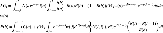
where f is the minimum age of enrollment in the system; L is the maximum age to which an individual biologically can live; N(a) is the number of plan members born a years ago; ϕ is the growth rate of the population of age 0 (which reflects fertility rates); l(a) is the survival probability to age a; R(b) is the share of the cohort that is retired by age b; P(b) is the average pension of all individuals in the cohort retired by age b; β is the contribution rate to the system; W t is the average covered wage at time t; w(.) is the age profile of wages; g is the growth rate of the average covered wage; ρ is the discount rate (which in this case should reflect the cost of capital); C(a)t is the average virtual capital accumulated by an individual of cohort a at time t; r* is the rate used to revalorize wages and index pensions (the IRR on contributions); and G(.) is the ‘G factor’ to transform the virtual capital into an annuity, which depends on the age of retirement, survival probabilities, and in this case the sustainable rate of return on contributions.Footnote 5
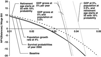
The sustainable IRR can be defined as the r* that solves FG(.)=0.Footnote 6 There is no close form solution to this equation, but we can see that r* will not only depend on the growth rate of the average covered wage (g) and the growth rate of the population of new borns (ϕ) – which in turn affects the growth rate of the population of contributors – but also survival probabilities and retirement patterns. To show this, Figure 1 graphs in the (FG, r*) space various realizations of equation (1). Each line corresponds to a combination of the growth rate of the average wage, the growth rate of the population, retirement probabilities, and the distribution of wages. The intersection of each line with the horizontal axis gives the equilibrium IRR. We see that the IRR increases with the level of economic growth, the population growth rate, and the fall in retirement probabilities by age. We also notice that a high rate of economic growth makes the lines quite steep, indicating that small changes in the IRR on contributions can cause the system to deviate from its long-term equilibrium. As a corollary, for a given IRR, a small change in the underlying macro and demographic conditions can also divert the system from equilibrium.Footnote 7 Clearly, outside the steady state the sustainable IRR would need to change at each point in time. The question is how.
Financing gap and the IRR
Note: The baseline scenario is built over the following assumptions: population growth of 1% per year; GDP growth of 3% per year; 2% growth in wages between ages; survival probabilities for Morocco in 2004; minimum retirement age 40 with 1% probability and maximum retirement age 75; no dropouts within age cohorts. The other lines represent deviations in one of the parameters from the baseline.
Source: Authors’ calculations.

The proposal developed here is based on an accounting framework ‘a la Swedish’ – although as shown below the actual indexation mechanism used in Sweden is not fully consistent with this underlying framework. The idea is simple: choose the IRR at each time t in a way that guarantees that the liabilities of the pension system are equal to its assets. The trick then is to properly define these liabilities, and, in particular, the assets of the ER pension system with pay-as-you-go financing.
The assessment of the liabilities of the system is straightforward. They are given by the present value of future pension payments to current retirees and to current contributors based on rights accrued to date.Footnote 8 In the case of a notional account system the value of the IPD is easily defined. It is given by the capital accumulated in the individual accounts plus the pensions in payment by age cohort multiplied by the annuity factor for that cohort.
The definition of assets is less intuitive. Clearly, a portion of the assets is given by the reserves of the pension plan – which can be equal to zero. The other part is the so-called pay-as-you-go asset, which is defined as the present value of future contributions minus the present value of pensions ensuing from these contributions (see Valdés-Prieto, Reference Valdés-Prieto2005a; and Robalino and Bogomolova, Reference Robalino and Bogomolova2006). The pay-as-you-go asset is positive when the implicit rate of return on contributions paid by the ER pension plan is below the rate used to discount future cash flows. This rate can be approximated by the rate of return that the pension institution receives on the investments of the buffer fund (a market rate). The difference between this rate and the implicit rate of return on contributions can be interpreted either as the ‘opportunity cost’ of saving in the ER plan or, put in other terms, an implicit tax on savings. Thus, in an ER system that is very generous, meaning it pays an IRR above market, the pay-as-you-go asset is negative.
Formally, in a solvent ER pension system with pay-as-you-go financing, the following equality needs to hold

where IPD t is the implicit pension debt at time t; PA t the pay-as-you-go asset and F t the value of the reserves (financial assets). So, in summary, in a solvent pension system, the pension promises that have been made to date have to be backed by financial assets and the future contributions net of pension rights accruing from them. As discussed above, a pension plan can operate with a negative pay-as-you-go asset, but not forever.
From equation (2) it follows that given the growth rate of the pay-as-you-go asset, call it a, and the growth rate of the reserves, call it r, we can solve for the allowable growth rate of the IPD at time t, holding constant system, economic, and demographic conditions. It turns out that this allowable growth rate of the IPD is the IRR that the pension system can afford to pay on contributions. It is the rate by which the pension plan can revalorize wages and index pensions. Indeed, as explained before, the IPD is made of accumulated contributions plus pensions in payment multiplied by the appropriate annuity factor. So the growth rate of the IPD is given by the growth rate of the stock of contributions and the stock of pensions in payments.
Thus, the IRR at time t can then be defined as

Hence, if we are able to obtain an accurate and simple estimate of the PA at each point in time, the expected sustainable IRR can be easily computed.
Before presenting a possible measure for the PA, we discuss how the approach proposed here to estimate the sustainable IRR differs from the Swedish system.
The analytical framework for the Swedish automatic stabilization mechanism is developed in Settergren and Mikula (Reference Settergren2005). The authors start by dividing the cross-section financing gap of the pension system (a simplification of equation (1)) by total contributions. In doing so, the authors indicate that they approximate the total financing gap that can be supported by one unit of contribution. The authors call this ratio the turnover duration (TD) and show, under simplifying assumptions, that the TD is equal to the money weighted average age of retirees minus the money weighted average age of contributors. The turnover duration times the contribution base then provides an estimate of what they call the contribution asset – different from the pay-as-you-go asset concept discussed above. Given information about the value of reserves, the authors calculate the ‘total assets’ of the system. When assets are equal or above pension liabilities, contributions/pensions are revalorized/indexed by the growth rate of the covered average wage. The indexation factor for pensions is also adjusted to take into account the interest rate imputed in the calculation of the annuity factors (see next section). When assets fall below liabilities a ‘balancing mechanism’ is activated and the growth rate of the average covered wage is multiplied by the funding ratio. Formally, we haveFootnote 9

where W t is the average covered wage at time t. Basically, the IRR is equal to the funding ratio multiplied by the growth rate of the average covered wage. If the funding ratio falls below one, then pensions and wages are indexed by less than the growth rate of the average covered wage (at least in the initial stage of ‘balancing’).Footnote 10
The same IRR is used to index pensions, but it is adjusted to take into account the discount rate imputed in the calculation of the annuity. Pensions are indexed by
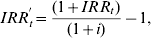
where i is the discount rate imputed in the calculation of the annuity.Footnote 11
There are several issues with this proposed balancing mechanism. A first issue is that the mechanism does not follow from first principles. It is unclear why an equation such as (4) was used instead of equation (3), where PA would have been replaced by TD∗C. The second issue relates to the interpretation of the turnover duration. Mathematically, the TD is not a good approximation of the pay-as-go asset, which is the relevant concept. For instance, the TD can increase as a result of an increase in life expectancy and that would be perceived as an increase in contribution assets when in fact that increase can reduce the pay-as-you asset as individuals receive pensions for longer. It is also not clear why the TD would provide an estimate of the financing gap that can be supported by a given contribution base. It could be informative regarding the level of the financing gap, but not necessarily whether it is sustainable. Actually, if the system is solvent, we would like the financing gap to be zero: liabilities would equate financial assets plus the pay-as-you-go asset. Finally, as the authors emphasize, the calculation of the TD is based on current information and the assumption of constant population growth. The TD would not capture future changes in the contribution base and therefore could overestimate or underestimate assets, thus paying an IRR on contributions that is too high or too low. In fact, Settergren (Reference Settergren2001) admits that long-term deficits in the buffer fund can arise in the case of long-term strains on the system like negative population growth. Section 4 will show that this is indeed what happens in the presence of exogenous shocks.
If the TD is to be replaced, how would the PA be computed? In the proposed approach, computing the PA is not very different from computing the IPD – which is also required in the Sweden scheme. For the IPD, we need estimates of G factors (annuity factors) by age. These depend on survival probabilities by age and assumptions about the future indexation of pensions (see discussion below on the discount rate used in the formula). For the PA, we need estimates of what we call Z factors – to keep similar terminologies – that give net assets for each age cohort. These Z factors also depend on survival probabilities and the market discount rate, but in addition estimates of retirement/dropout probabilities, the current age profile of wages (also used for the calculation of the TD), and the expected growth rate for wages. So computing the expected PA is not more difficult than computing the TD or the IPD.
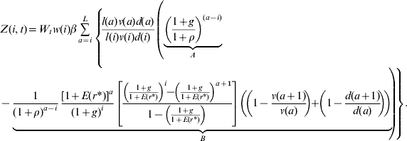
The Z factor for a cohort of age i at time t, is given by
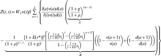
where v(a) gives the probability of not being retired by age a, d(a) the probability of not having dropped out of the system by age a, and E(r*) gives the expected rate of return on contributions. Basically, expression A captures the present value of contributions paid at age a, and expression B the pensions (and lump sum) paid to new retirees (and dropouts) at age a.Footnote 12 Then the pay-as-you-go asset at time t is

where N(a, t) are the contributors of age a at time t, dN(b, k) the new entrants of age b at time k, and T the planning horizon.
We can argue that having estimates of future entrants, the growth rate of the average wage, and the expected rate or return on contributions is complicated. The proposal developed here assumes that past trends hold. The E(r*) is estimated by an average of past IRRs and new contributors by age can be projected given past information on new entrants and their age distribution. A virtue of the PA is that it is forward looking. Basically, it tries to anticipate the effects of shocks that occur today on the future flows of net contributions. Clearly, the past is not necessarily a good predictor of the future. Hence, when calculating the PA of a system in year 2005, we would miss the impact of unknown phenomena that take place, say, one decade from now. Let us assume, for instance, that the unknown shock is a permanent drastic drop in coverage rates that takes place suddenly – unannounced. Estimates of the PA in the years prior to the shock would overestimate its true value (i.e., wages and pensions would be revalorized/indexed by a rate that is too high). Nonetheless, as soon as the shock takes place, and the system identifies that is permanent, its short and long-term effects would be incorporated in the calculation of the IRR, making up for previous overadjustments. We also emphasize that those shocks that take place far into the future have a small impact in the current value of the PA.
Computing annuities and indexing pensionsFootnote 13
There is an important decision to be made regarding the calculation of annuity factors and the type of indexation mechanism used for pensions. Often decisions at these two levels are disconnected and, as shown in Section 4, this is problematic for an NA system without the appropriate stabilization mechanism.
If in practice pensions are going to be indexed by the IRR (or rough proxies such as wages or GDP growth rates), which is also the rate used to revalorize wages, then the annuity factor should not incorporate a discount rate. In other words, the pension would be simply equal to the notional capital accumulated in the individual account divided by the life expectancy at retirement. On the contrary, if pensions are solely going to be indexed by prices, the annuity factor should incorporate in the calculation the expected IRR. Basically, if pensions are only going to be indexed by prices then they should be higher from the start. If they are going to be indexed by the IRR, then they should be smaller.
It is possible to define the correct indexation factor π given the sustainable IRR and the discount rate i used in the calculation of the pension. Factor π needs to solve

where C R is the capital accumulated in the individual account at the time of retirement. The expression in brackets is the value of the initial pension calculated on the basis of a discount rate i. Equation (7) states that if, ex-post, the pension is going to be indexed by π, the present value should still be equal to C R. It is easy to show that for equation (7) to hold, the following needs to be verified for any b
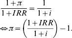
Clearly, if the IRR itself is not sustainable, then this correction will not solve the problem of financial sustainability.
In practice, policymakers would need to adopt an indexation mechanism that is consistent with the annuity formula but this is seldom the case. Introducing a discount factor in the calculation of the annuity is a way to guarantee higher pensions up front. At the same time, policymakers might face pressure to keep the growth of pensions in line with the growth in wages.
If the system incorporates a stabilization mechanism such as equation (3), then there is flexibility in terms of whether or not a discount factor is used in the calculation of the annuity. Indeed, the stabilization mechanism will ensure that the IRR that is used to revalorize wages and index pensions after the discount factor was taken into account brings the pension system to a sustainable path. The higher the discount rate used in the calculation of the annuity, the lower the IRR that the system will pay (i.e., the lower the rate used to revalorize and index pensions). If no discount factor is used, then the system will pay the maximum IRR other things being constant. Because the IRR is the rate that should be used to discount the flow of contributions and pensions, this approach ensures that all individuals within a given age-cohort receive the same implicit rate of return on their contributions – albeit one that moves over time – regardless of wages and contributions histories.
With no stabilization mechanism, however, the discount factor might be too high relative to the allowable IRR – which as seen before changes over time – and it will not be possible to correct. This is shown in Section 4. One alternative in this case, is not to include a discount factor in the calculation of the annuity, but to guarantee full indexation of pensions on the basis of the system IRR. However, it can be shown that under general conditions individuals – at least those who have limited access to financial markets and face stringent borrowing constraints – would be better off if a discount rate is introduced up front and the pensions are indexed by prices.Footnote 14
3 Simulating the robustness of alternative rules for the IRR of the system
To study the dynamics of an ER pension system with pay-as-you-go financing under alternative rules for the IRR, we use a simple one-sector macro model that incorporates a notional account pension scheme (see Appendix 2 for a formal description). For simplicity, and given that the focus is to analyze the dynamics of the IRR, economic growth and the savings rate of the economy are exogenous in the model. Future extensions should study the behavior of the pension system with endogenous savings. The dynamics of wages and the market interest rate, on the other hand, are endogenous in our model. This model provides a mechanism to ensure internal consistency regarding changes in pension system design, macroeconomic trends, and demographic trends. For instance, simulated fluctuations in GDP growth will affect the pension system through changes in wages and the interest rate – a recession is accompanied by higher interest rates. Similarly, retirement and survival probabilities will affect the economy through a change in the size and age composition of the labor force, which in turn affects wages and the interest rate. Coverage and labor supply, however, are not affected by changes in the macroeconomy or pension system parameters.
We use the model to understand how various rules for the evolution of IRR on contributions affect the dynamics of the pension system. In particular, cash balances and reserves levels. If the earnings-related system is financially self-sustainable, then the value of reserves should never be negative – or at least not for an extended period of time.
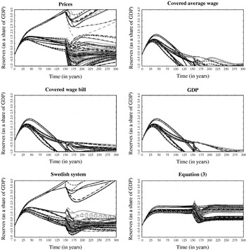
We consider six rules to determine the IRR across a large number of economic and demographic scenarios: (i) wages are revalorized by the growth rate of the average covered wage and pensions are indexed by prices (i.e., growth is zero in real terms); (ii) the IRR is equal to the growth rate of the average covered wage and it applies to wages and pensions; (iii) the IRR is equal to the growth rate of the covered wage bill; (iv) the IRR is equal to the growth rate of GDP; (v) the IRR is based on the Swedish system (equation (4)); and (vi) the IRR is based on the proposal developed in this paper (equation (3)).Footnote 15 We also take into account two different methods to compute the annuity; with and without a discount factor.
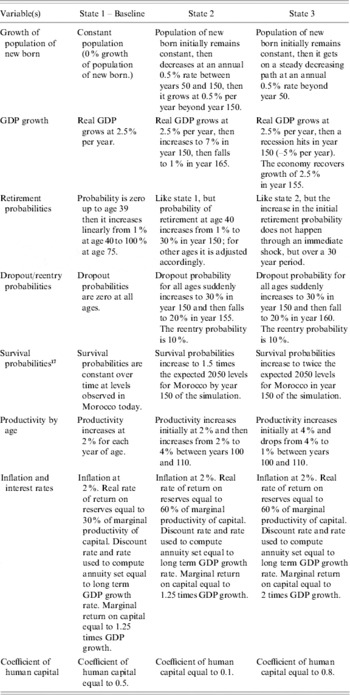
As for the scenarios, we consider combinations of eight blocks of variables: (i) population growth; (ii) GDP growth; (iii) retirement probabilities; (iv) drop-out/reentry probabilities; (v) survival probabilities; (vi) productivity by age; (vii) inflation and interest rates; and (viii) the coefficient of human capital in the production function. Basically, each of these variables/groups of variables is allowed to be in one out of three states.Footnote 16 The various states are described in Table 1 and have been selected to put the pension system under high stress and assess its resilience. The deviations from state 1 can be considered as shocks to the system. As a general rule, they are introduced at a point in time when the system has already reached a great degree of maturity.
State for key model variables

Note: Initial population of new born is 1,000. Initial GDP per capita is 100 units. Initial level of capital is calibrated to achieve targeted, long-term, marginal return on capital. Minimum age to enter the labor force (f) set at 20 years.
We discuss the results of the simulations in three parts. First, we look at the dynamics of funds reserves under each of the rules for the IRR across a random sample of 100 scenarios evolving over a period of 300 years. Then, for each of the indexation rules, we look at the distribution of the following outputs: (i) the value of the reserves as a share of GDP in year 150 and year 300; (ii) the value of the cash-balance as a share of GDP in year 150 and in year 300; (iii) the average IRR for the period t∊[150,300]; and (iv) the maximum value of the reserves as a share of GDP during the entire simulation period. Finally, we analyze the sensitivity of the steady level of fund reserves and the IRR to changes in selected model variables.
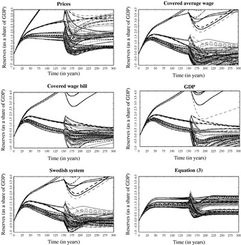
We first discuss the simulations where the calculation of the annuity factor does not include a discount rate. The results show that only the new proposal developed in this paper and the ‘price indexation mechanism’ – that is salaries (contributions) revalorized by the growth rate of the covered average wage and pensions indexed by inflation – are capable of avoiding extended periods of negative reserves (see Figure 2). Like the other revalorization/indexation mechanisms, however, price indexation is not stable in the sense that for some of the scenarios, assets (reserves) accumulate without bound. This implies that the system is penalizing workers by paying an IRR below the sustainable level, essentially a higher implicit tax on savings than what the system requires.
Dynamics of the reserves to GDP ratio when the annuity formula does not include a discount rate
Source: Author's calculation.

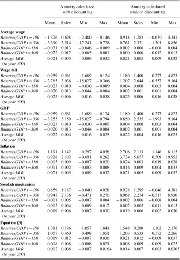
This being said, none of the indexation mechanisms is systematically unsustainable when the annuity is calculated without discounting, simply because there is ‘more room’ in this case to index pensions. The average value of reserves over the 100 random combinations of states is positive for all the six indexation mechanisms both in year 150 and 300. The mean cash balance is positive for all the indexation mechanisms in year 300, and positive or slightly negative in year 150 when some of the shocks take effect (see Table 2).
Descriptive statistics for selected outputs

Source: Authors' calculations.
The Swedish mechanism clearly outperforms the average wage growth, the covered wage bill growth and the GDP growth indexation mechanisms in terms of keeping positive reserves. However, the Swedish system exhibits a tendency to over-accumulate assets when population growth is positive, while the balancing mechanism is vulnerable against a shrinking population. Indeed, several combinations of states that include long-term negative population growth put the Swedish system into an unsustainable path (see the Appendix 3 for a comparative sensitivity analysis of the Swedish system and the new proposal, including various population growth scenarios).
As pointed out already, the inflation adjustment rule is robust as pensions are indexed, on average, by an IRR below the sustainable level. In a way, the protection against ‘system bankruptcy’ comes at the cost of high implicit taxes on savings. We also notice that price indexation displays a higher variance in the level of reserves.
The proposal developed in this paper is the only mechanism that avoids extended periods with negative reserves and converges towards a sustainable steady-state in all the scenarios.
When a discount rate is introduced in the calculations of the annuity, the results are very different (see Figure 3).Footnote 18 The average wage growth, the covered wage bill growth, and the GDP growth indexation mechanisms become unsustainable in all the scenarios. This is not surprising since, in essence, pensions are being indexed twice. First, ex-ante, at the time of calculating the pension – since the annuity factor already incorporates a discount (i.e., indexation) factor – then each time pensions are paid.
Evolution of the reserves to GDP ratio when the annuity formula includes a discount rate
Note: The discount rate used in the calculation of the annuity is equal to the long-term growth rate of the economy.
Source: Author's calculations.

Price indexation behaves better since, as discussed in the previous section, the calculation of the annuity with a discount factor (expressed in real terms), is consistent with price indexation. The problem is that the discount rate used in the calculation of the annuity factor is not necessarily the sustainable rate. Price indexation therefore struggles with the higher level of initial pensions without any mechanism for correction.
Only the Swedish indexation mechanism and the new proposal based on equation (3) are equipped to adjust the indexation mechanism in relation to the discount factor used in the calculation of the annuity. The Swedish mechanism, when the balancing mechanism is not activated, actually behaves like price indexation if the growth rate of the average wage is equal to the discount rate used in the calculation of the annuity factor. The stabilization mechanism, however, is not sufficient to deal with periods of negative population growth rate and therefore there are still scenarios where the reserves of the system become negative.
The rule proposed in this paper, on the other hand, never generates negative reserves and converge in all cases to a stable steady state. In part, this is because the proposed algorithm also takes into account the impact of the discount rate in the pay-as-you-go asset (i.e., other things being equal, the higher the discount rate the lower the pay-as-you-go asset).
To gain more insights into the results of the simulations, we look at summary statistics for key output variables (see Table 2). There are several interesting observations. First, the mechanism proposed in this paper and the price indexation mechanisms are the only ones capable of ensuring positive reserves levels at the end of the simulation horizon. Even the Swedish system runs into debt by year 300 to the amount of 57.2% of GDP under the worst set of ‘environment conditions’. We also observe that both the range and the variance of the level of reserves are the smallest under the indexation rule following equation (3). The proposed mechanism ‘downward adjusts’ the IRR in straining situations, but even then it does not push the IRR into the negative. This is an important message from the simulations because; conceptually, negative IRR paths are consistent with equation (3) under certain circumstances. These, however, would be difficult to implement at the practical level.
To better understand the interactions between the macroeconomy and the pension system under the Swedish and the proposed indexation mechanisms we simulated the effects of isolated changes in selected model variables on the steady-state levels of the fund reserves, cash balances, the path of the funding ratio and the IRR. The results are presented in Appendix 3. The main messages from the analysis can be summarized as follows.
First, it is interesting to observe that the Swedish system generates higher funding ratios than the proposal developed in this paper. This reflects the difference in the methodology used to calculate the pay-as-you-go asset. The new proposal implements a direct estimation of this asset. The Swedish system approximates this asset through the level of contributions and the turnover duration. The results suggest that this methodology tends to overestimate the pay-as-you-go asset.
Second, the new proposal generates more rapid adjustment paths in response to shocks. Fluctuations in adjustment paths are also less pronounced than in the case of the Swedish system. This is because the Swedish system is sensitive to changes in the growth rate of the covered average wage, which is in turn very sensitive to economic shocks. The new proposal relies on the pay-as-you-go asset, which dampens these fluctuations by also taking into account the effects on the dynamics of the population of contributors and beneficiaries.
Third, the Swedish system is very sensitive to changes in the growth rate of the population and there are cases where the system is not able to avoid negative reserves. This can also be explained, in part by a revalorization based on the growth rate of the covered average wage, which will be higher when population growth rates – and therefore the growth rate of the labor force – fall.
Finally, while the funding ratio falls when retirement probabilities, drop-out probabilities, and survival probabilities increase, the reduction is not always sufficient to activate the balancing mechanism. This implies that the revalorization continues to depend on the growth rate of the covered average wage and that pensions are indexed by the growth rate of the average wage adjusted by the discount factor. When retirement probabilities increase, wages and the IRR go up – since labor supply falls. When survival probabilities increase, wages and the IRR go down – since the labor force increases. Only when the shock is driven by an increase in drop-out probabilities, which is less important for the dynamics of wages, at least in the short term, the IRR is more responsive to the funding level.
By looking at the IRRs generated by the Swedish system, we can see that these are often above the IRRs generated by the new proposal, which, as shown in the previous section, preserve the solvency of the system (i.e., liabilities are equal to assets).
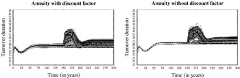
The dynamics of the pension plan under the Swedish stabilization mechanism deserves further analysis. As previously discussed, the IRR paid by the system is roughly equal to the funding ratio times the growth rate of the average wage, when the balancing mechanism is on. The funding ratio in turn depends on the turnover duration that, when multiplied by total contributions, is supposed to provide an estimate of the assets of the plan – excluding the reserves. Because the turnover duration depends on average contributions and average pensions by age, it is sensitive to changes in retirement and dropout probabilities. It is also sensitive to changes in the age–wage profile and shocks that affect the marginal productivity of labor. Figure 4 displays the evolution of the turnover duration across the same 100 scenarios presented above. We observe that for several of the scenarios, those where macroeconomic, behavioral, and/or demographic shocks are observed, the TD is subject to important changes. These fluctuations, however, are often positive, indicating a higher level of assets. Therefore, for several of the shocks, assets would actually increase and the balancing mechanism would not be activated.
Dynamics of the turnover duration in the Swedish stabilization system
Source: Authors' calculations.

4 Introducing government-indexed bonds
The proposal to invest the contributions of the pension plan into government bonds to ensure financial sustainability and make pension liabilities explicit was, to our knowledge, first introduced by Buchanan (Reference Buchanan1968). Other theoretical discussions include (Auerbach and Kotlikoff, Reference Auerbach and Kotlikoff1987; Sinn, Reference Sinn2000). There have also been proposals for applications of the concept (see Palacios and Sin, Reference Palacios and Sin2002) and Robalino et al. (Reference Robalino, Whitehouse, Mataoanu, Musalem, Sherwood and Sluchinsky2005a, Reference Robalino, Hinz, Sluchinsky, Dorfman and Mataoanub), but the mechanics and fiscal implications have not been fully spelled out.
The idea is that, under the certainty case, a well-designed ER system can be made financially self-sustainable if past wages (or contributions) and pensions are revalorized/indexed by the rate of return on the government bonds. Indeed, in this case, the value of the bonds held by the pension system is equal, at all points in time, to the pension liabilities.Footnote 19 In addition, government bonds can serve other purposes: (i) improve fiscal management and provide incentives for a more careful choice of the parameters of the pension system, since the liability is now explicit; (ii) facilitate the transparent financing of the IPD of a pre-existing system; and (iii) reduce the risk of capital loss if workers savings are managed by a public institution where governance, accountability and investment policies are week. If at some point in time the government bonds become tradable, then this policy can also facilitate the transition to a defined-contribution fully funded pension system.
There are two problems with the original idea however. First, when there is uncertainty regarding the evolution of demographic parameters, pension liabilities can increase – for instance due to an unexpected increase in life expectancies – while the value of the bonds remains constant. This would generate a liability within the pension system that is not ‘funded’. This mismatch would need to be corrected by adjusting pensions (retirees face the burden), by introducing a temporary contribution that does not accrue pension rights (a tax on labor), and/or general revenues (tax payers face the cost).
A second problem is that, as shown in Section 2, the sustainable IRR that the ER system can afford to pay on contributions (and can use to index pensions) could be above the growth rate of return on the bond, which is presumably below the rate of return of the market portfolio. This is because of the presence of the pay-as-you-go asset. By paying a rate of return below the sustainable rate, the share of bonds in GDP could increase too fast and plan members would be penalized.
The implication is that even if contributions are allocated to government bonds, it is desirable that the IRR of the system be calculated on the basis of equation (3) above.
In the remainder of this section we discuss how the proposed system could be designed, what are the considerations to keep in mind, and what would be the fiscal implications. In particular, we address the following questions: (i) what types of government bonds could be used; (ii) how the ratio of bonds to GDP would evolve; (iii) how bonds should be issued/repaid and what would be the proper accounting within the fund; and (iv) what would happen if the bonds were traded.
Types of bonds
In principle, any type of government bond could be used to invest the contributions of the ER system. The choice is both important from a fiscal point of view and from the perspective of the pension fund. First, any financial arrangement needs to be fiscally sustainable or the pension system would not be secure. Second, the yield on the bond should be a good proxy for the IRR of the system.Footnote 20
Given the desire to keep the size of the government liability manageable in relation to government revenues – which are used to serve this liability – one natural alternative to consider is the issuance of GDP-indexed government bonds.Footnote 21 As discussed in Borensztein and Mauro (Reference Borensztein and Mauro2004) these bonds can protect the government against increases in interest rates that would raise debt/GDP ratios, in exchange for a relative small premium.Footnote 22 Over the long term, GDP growth is also a good proxy for the sustainable IRR of the system.
Implementation and accounting
How would bonds be issued and priced, and how would the pension fund manage the accounts? The idea is that every 6 or 12 months, the cash surplus of the pension fund would be invested in GDP-indexed government bonds (in the transition period cash balances could take the form of bank deposits). These bonds are similar to ‘plain vanilla’ bonds except that the coupon rate is variable. It varies as a function of the growth rate of the economy. In the general form, the coupon rate at time t would be defined byFootnote 23

where  t is the coupon rate paid on pure vanilla bonds of identical maturity at the time of the issuance of the GDP-indexed bond, Ω is a premium that investors could demand given more variance in the bond, α is the parameter of indexation, g is the GDP growth rate at time t, and
 is the GDP growth rate expected at the time of issuance. So the value of the coupon is calculated each year on the basis of the expected and observed growth rate of the economy.
By design, pension liabilities are always backed by government bonds. This would imply that pensions are covered out of revenues from the bonds and that all new contributions are invested in new bonds. In practice, of course, this does not have to be the case. The pension fund would invest in government bonds its operating balance (including revenues from coupon payments and bonds that mature). When the revenues from bonds that mature exceed pension payments – this can happen as the maturity rates of the bonds are not necessarily aligned with retirement patterns (are shorter in this case) – the surplus is reinvested in new government bonds. On the other hand, if pension payments are above the value of bonds that mature – meaning that maturities were too long for retirement patterns, contributions can cover the difference. From the point of view of the pension fund, this operation is equivalent to having sold part of the bonds to cover the gap, while buying the equivalent amount of new bonds with the new contributions.
The accounting of the proposed system is simple. On the asset side of the balance sheet the pension fund keeps track of the pay-as-you-go asset and the stock of bonds – initially registered at face value since they are not traded. This stock moves as a function of the repayments and the balance of the fund. On the liability side of the balance sheet, the pension fund tracks separately the notional individual accounts (remunerated on the basis of equation (3)) and the mathematical reserves for pensions in payment (indexed on the basis of equation (3)).
When individuals retire the notional capital accumulated in their individual account is transferred to the mathematical reserves. Alternatively, if the system outsources the issuance of annuities, the lump sum capital would be transferred to the selected insurance company and subtracted from the IPD.
Fiscal sustainability
How would the bonds/GDP ratioFootnote 24 evolve over time? The evolution of this ratio will depend on the growth rate of GDP, which affects the growth of the stock of bonds, as well as new issuances. New issuance will take place as long as contributions are higher than pensions. To see this, it is useful to write the cash flows that the government will require annually for serving bonds obligations. It is given by

where B t–1 is the stock of bonds at year t–1, εt–1 the share of bonds that mature, C t are total contributions at time t, and P t are total pensions. The expression in brackets gives the net balance of the pension fund. We see that when contributions are higher than pensions, the government is not only rolling over payments, but also issuing new bonds. When contributions equal pensions, the government can just roll the bonds over. When contributions are below pensions, it is time for the government to start financing part of the bonds out of general revenues. This is important to emphasize. Bonds have to be repaid out of general revenues; the pay-as-you-go asset goes to the plan members, not to the government.
As such, the analysis of sustainability of GDP-indexed government bonds linked to the pension system is no different from the analysis of sustainability of other forms of public debt. The only change is that the analysis needs to take into account the future cash-balance of the pension fund, which allows the government to roll-over the bonds.
So where to stop? When the new ER system replaces an ER system that had a large IPD and the government is cash-trapped, choices would be limited. New issuances of GDP-indexed government bonds would be used to pay the pensions of the old-system, in effect making its implicit debt explicit. Above and beyond that level, however, the government does have several options.
One option is to allocate revenues from bond issuances to the repayment of other debt (with higher yields) or investments in liquid financial assets.
Another option, not mutually exclusive, is to reduce the level of borrowing by allowing the pension fund to diversify investments. Basically, part of the reserves would be allocated to a diversified portfolio of financial assets. This option can go hand in hand with the tradability of the government bonds. Clearly, before implementation the appropriate governance structure would need to be in place to ensure that funds are managed in the best interest of plan members.
In any event, rating agencies would need to monitor the public debt and penalize governments where GDP-indexed bonds linked to the pension system start to accumulate well beyond the level of implicit debt of the old-system, without reductions in other sources of government debt. The idea is for the new instrument to be an alternative source of financing rather than an additional source of financing. At the same time, rating agencies should not penalize countries that make the liabilities of the pension system explicit (even if not tradable). On the contrary, rating agencies would need to compensate countries that control the accumulation of unfunded liabilities of earnings-related pension systems through the issuance of GDP-indexed bonds and the adoption of well-designed benefit formulas.
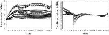
To illustrate the potential fiscal impact of linking the contributions of an ER system to government-indexed bonds, we simulate the net balance of the pension fund, which as shown above is equivalent to the amount of general revenues necessary to repay bonds at a given point in time. Since in our model GDP growth is exogenous and not subject to stochastic shocks, we use a simple type of bonds where r=0, Ω=0, α=1, and =r. So, the coupon rate is exactly equal to GDP growth. We implement the simulations using the revalorization/indexation mechanism defined by equation (3). The results are presented in Figure 5. The results show that the system can generate negative cash balances for the pension fund. The size of the short fall between contributions and benefits depends on the nature of the underlying shocks. In most cases, the short falls should be covered by the value of the coupons and the bonds that mature. In some cases, as a result of a large unexpected shock, short falls can be large. In the scenarios that we have considered, which, as said before, set very high standards for the pension fund, the deficit in the case of the system with a stabilization mechanism could be as large as 7–8% of GDP. Clearly, dealing with large shocks is a challenge for any pension system. In this case, there are also various ways to proceed. One is for the pension fund to request advance payment of part of the stock of bonds. If the government faces liquidity constraints and/or was affected by the same shock that hit the pension fund, it could borrow without changing the fiscal stance – it would replace one type of debt by another. The other possibility is for the pension fund to trade government bonds. This option of course has implications for the value of the bonds and deserves a separate discussion.
Fiscal impact of GDP-indexed bonds with stabilization mechanism pure
Source: Authors' calculations.

What happens when the GDP bonds owned by the pension fund are traded? In the unlikely case that the yield demanded by investors was exactly equal to the coupon rate, nothing would happen. The market price of the bonds would be equal to the face value of the bonds. In reality, things are different. Investors will hold GDP-indexed government bonds as long as these generate a premium that is ‘worth’ the risk; not only the risk embedded in the variable coupon (which depends on GDP growth), but also the country risk, the risk of default by the government, and the liquidity risk that accompanies a market that has not yet developed. Country risk and risk of default are already captured by standard government bonds. The question is what the extra premium to accept the extra risk is. Under certain assumptions regarding the behavior of investors, this premium would be a function of the expected rate of return on a risk free asset, the expected growth rate of GDP, and the covariance of this growth rate with the ‘market portfolio’. Bottom line, the higher the country risk, the higher the perceived probability of default, the lower the expected growth rate of the economy, and the higher the covariance between the growth rate of GDP and the market portfolio, the higher the premium requested from investors (the higher Ω). The higher the premium, the lower the price they are willing to pay for the government bonds. Hence, it can be the case that when the pension system trades the government bonds it also abruptly loses the value of the assets. This is particularly true at times of crisis, but it can happen in normal times as well, simply because when the government issues the bonds it is not paying the risk premium that markets would have demanded (Ω=0). One possibility to solve this problem is to trade a portion of the bonds from the beginning or, even better, to have a parallel issuance from the start. In this way, the pension fund will also have a benchmark to price the bonds.
5 Discussions and policy implications
In this paper we have proposed a mechanism to design a financially sustainable and secure earnings-related scheme with pay-as-you-go financing. The mechanism combines the investment of reserves in GDP-indexed government bonds with a new measure for the rate that the plan should use to revalorize contributions and index pensions (i.e., the sustainable implicit rate of return on contributions). This rate is a function of the growth rate of the reserves (in this case the stock of government bonds) and the so-called pay-as-you-go asset of the system.
We argue that the proposed approach has several virtues: (i) it eliminates the risk of mismanagement of the funds that inevitably accumulate during the first couple of decades, and which are necessary to finance pensions when the system matures; (ii) it improves fiscal management by making the implicit liabilities of the new system explicit; (iii) it provides incentives and controls for policymakers to respect rules that ensure the long-term financial sustainability of the ER system; (iv) it facilitates the transition to the ‘new’ system in countries where the ‘old’ ER system has accumulated a large IPD; and (v) facilitates the transition to a defined-contribution funded scheme.
While the proposed arrangements could serve any ER system, they are better suited for notional account systems that establish a clear link between contributions, the rate of return on these contributions, and pensions. In addition, this system has a simple characterization of the IPD: the sum of notional capital in the individual accounts, plus pensions in payment by age cohort times the annuity factor of that cohort.
There are, however, issues that could affect implementation and that deserve further attention. A first set of issues has to do with the mechanism used to compute the IRR on contributions. One is that the value of the pay-as-you-go asset will depend on expectations about the initial IRR and the growth rate of wages – this could give room for discretion. The second is that financial sustainability might require that in some circumstances the IRR be negative. Since this rate is used to index pensions the approach would require that individuals accept the possibility of having their pensions drop in absolute terms. This is unlikely to be appealing to individuals. One way around this is to have pension which are only indexed by inflation but that in the calculation include an implicit interest rate. The stabilization mechanism suggested here would then ensure that the IRR paid on contributions is properly adjusted.
Another question is the level of sophistication of the scheme. Some might consider that the proposed method to compute the IRR is complex and that pensions systems in middle- and low-income countries will not have the institutional capacity to implement. Our position is that creating this institutional capacity should be part of any reform program – including one that intends to keep defined-benefit provisions intact. In all cases, information and administrative systems should be upgraded to ensure that the pension fund can properly track the contributions of plan members and other individual characteristics. In all cases, the managers of the pension plan should have access to up-to-date financial information, including the evaluation of the liabilities of the plan.
A third set of issues has to do with fiscal implications. In the paper, we argue that the fact that the government mandates a pension scheme that is not fully funded automatically creates an implicit liability. The proposed arrangement does not change the nature of that liability – it simply ‘registers the liability in books’. Furthermore, because the bonds are a debt of the government with a public institution they cancel out in the reporting of the consolidated public debt.Footnote 25 This being said, the analysis of sustainability of the public debt should take into account the accumulation of GDP-indexed bonds with the pension fund. This is simply because, as shown in the paper, the sustainability of the pension plan does depend on the ability of the government to serve the bonds. So, the existence of these bonds imposes constraints on the use of other forms of financing. Because the bonds are linked to GDP and at least initially do not require a premium, they actually could be a very interesting source of financing for the public sector. Still, there are several questions that require further analysis. For instance, how would the existence of the bonds change the structure of the public debt and the spreads on other bonds? How does the cost of the indexed bonds compare to other debt instruments? Will the government be able to meet the demand for bonds? How will investors react to the accumulation of GDP-indexed bonds? When should the bonds be allowed to be traded? These are important questions that fall outside the scope of the paper and that should be considered in future research.
Appendix 1 – Derivations
Derivation of P(b)
The average virtual capital accumulated by an individual of a cohort a at time t who retires at age i with i⩽b

If we turn this virtual pension capital into an annuity, the average pension payment of an individual of cohort a retiring at age i with i⩽b in the period when the individual reaches age b (i.e. at time t+b−i) is as follows

Recall that R(b) is the share of the age cohort (any age cohort given constant retirement probabilities) that retired by age b. Consequently [R(i)−R(i−1)]/R(b) is the share of R(b) that is associated with those who retired between ages i−1 and age i. Consequently the formula for the average pension payment at time t, calculated in relation to all individuals in age cohort a who retire at or before age b, can be constructed by integrating the previous formula over all retirement ages between a and b and including relative weights of the population retired between ages i and i−1

Derivation of Z(i, t), the Z factor
The present value of future contributions assuming that that age profile of wages function w(.) is consistent with the average growth rate of the covered wage bill g on the individual level is as follows

The joint probability that an active person of age a either retires or drops out by age a+1 is [1−v(a+1)/v(a)]+[1−d(a+1)/d(a)]. Assuming that the virtual pension capital to be accumulated beyond age i is to be used to purchase an annuity at retirement/drop-out age a, the present value of pension benefits to be earned through future contributions by age cohort i is as follows
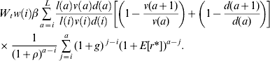
Based on (A1-4) and (A1-5) and applying the sum of geometric series formula, we have that
Appendix 2: The macro model
The formal description of the model is presented in Box A2-1. The various equations are organized in five blocks: population; labor force; output, wages and interest rates; plan members; and revenues and expenditures of the pension system. We briefly discuss each of these blocks.
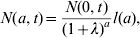
The first two equations define the dynamics of the population (N). Basically, the population of new born is assumed to grow at an exogenously defined rate (λ). Given survival probabilities by age, the total number of individuals in each age cohort is computed at each point in time.
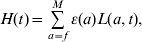
Equations (A2-3) and (A2-4) determine the evolution of the labor force (L) and human capital (H) respectively. The labor force is made of all individual of age a⩾f (where f is the minimum economically active age) and who have not retired. Thus, in equation (A2-3), v(a) is the probability of not being retired by age a. The implicit assumption is that participation rates are 100% for all ages. This simplification does not affect the results from the analysis. As for human capital, it is defined as the sum of the labor force by age-cohort multiplied by their productivity/quality, which will affect the level of wages by cohort. Thus, in equation (A2-4), ε(a) captures the age–wage profile.
Box A2-1 Model for analysis of robustness of rules on IRRs
Initial and total population by age-cohort:(A2-1) (A2-2)Labor force by age cohort and human capital:(A2-3)(A2-4)Output, productivity, wages and interest rate:(A2-5)(A2-6)(A2-7)(A2-8)(A2-9)(A2-10)(A2-11)Contributors, dormants, and old-age pensioners:(A2-12)(A2-13)(A2-14)Individual accounts by age cohort, total pensions by age-cohort, and total reserves:(A2-15)(A2-16)(A2-17)




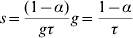







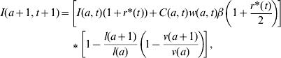


Equations (A2-5) to (A2-11) determine output (Q), the savings rate of the economy (s), capital (K), total factor productivity (A), wages by age (w(a)), and the market interest rate r m. The underlying assumption is that output is generated by a Cobb–Douglas function that incorporates human capital, physical capital, and total factor productivity. The growth rate of output (g) is defined exogenously. The savings rate of the economy is defined in a way that, in the steady state, the level of capital ensures that the market interest rate (the marginal productivity of capital) equals gτ, where τ is defined exogenously. This last parameter is basically the ratio between the real market interest rate and the growth rate of GDP. So, (1−α)/ (gτ) is the capital output ratio. Wages (by age) and the market interest rate are then computed under the assumption of full employment as the marginal productivity of labor (by age) and capital respectively. In equations (A2-6) to (A2-11), α is the share of human capital in production.
The evolution of the stocks of contributors (C), dormants (D; individuals who stopped contributing but have pension rights), and old-age pensioners (O) are given by equations (A2-12) to (A2-14). We assume that all individuals in the labor force join the pension system at the beginning of the simulation (C(a,1)=L(a,1)) and that all new entrants to the labor force join the pension system at time t>1 (C(f, t)=L(f, t)). From there the stock of contributors, dormants, and old-age retirees respond to survival probabilities l(.), dropping out probabilities d(.), reentry probabilities b(.), and the probability of continuing in the labor force instead of retiring v(a). Notice that individuals who drop out of the pension system, do not drop out of the labor force. In this model, these individuals continue working and earning a salary – they simply do not contribute.
Finally, equations (A2-15), (A2-16), and (A2-17) give the dynamics of the capital value of the individual accounts and total pension expenditures for each age cohort, as the total reserves of the system. The new symbols in these two equations are: r*, the revalorization/indexation factor for wages/pensions (i.e., the internal rate of return on contributions); β, the contribution rate; G(a, t, i) the annuity factor at age a and time t, that depends on the interest rate i (a policy parameter); and η which gives the rate of return on investments of the reserves relative to the market interest rate.
The notional capital value of pension accumulation over a period for a given age cohort incorporates the previously accumulated capital and its returns plus current contributions of the surviving and not yet retiring portion of the given age cohort. Equation (A2-15) takes into account that contributions are paid continuously throughout the year. The total pension amount paid to an age cohort evolves from period to period in accordance with (A2-16). The surviving portion of previously retired individuals of the cohort will receive pensions indexed by the IRR and the accumulated pension capital of new retirees is turned into annuities. The reserves of the pension system (A2-17) evolve over time in accordance with the returns/borrowing costs on the previously available reserves and the sum of the balances of current contributions and ‘newly exchanged’ pension annuities for all age cohorts. These balances are augmented by the investment returns/borrowing costs assessed on their continuous flows during the applicable year.
Appendix 3 – Sensitivity/robustness analysis
The following figures compare the sensitivity/robustness of the Swedish automatic balance mechanism and that of the indexation mechanism of the proposal developed in this paper towards certain demographic shocks, holding all other factors constant. The baseline simulation path scenario corresponds to state 1 in Table 1. The deviating paths are identified in the figure legends and they correspond to the alternative states defined in Table 1. The sensitivity analysis towards population growth and survival patterns include one additional path each. All the simulations here apply annuity calculations with discounting.
Sensitivity analysis – population growth scenarios
Evolution of the reserves and balance of the pension system as a share of the GDP, the funding ratio and dynamic internal rate of return of the pension system under the Swedish automatic balance mechanism and the new indexation proposal

Sensitivity analysis – survival pattern scenarios
Evolution of the reserves and balance of the pension system as a share of the GDP, the funding ratio and dynamic internal rate of return of the pension system under the Swedish automatic balance mechanism and the new indexation proposal

Sensitivity analysis – retirement probability scenarios
Evolution of the reserves and balance of the pension system as a share of the GDP, the funding ratio and dynamic internal rate of return of the pension system under the swedish automatic balance mechanism and the new indexation proposal

Sensitivity analysis – drop-out probability scenarios
Evolution of the reserves and balance of the pension system as a share of the GDP, the funding ratio and dynamic internal rate of return of the pension system under the Swedish automatic balance mechanism and the new indexation proposal