1 Introduction
The way in which sand is moved by the action of water waves is still puzzling scientists and coastal engineers. In near-shore shallow environments, large near-bed wave orbital velocities, asymmetric waves, breakers and swash run-up/run-down generate a variety of complex destabilizing effects on the bed sediment (e.g. Bailard Reference Bailard1981; Conley & Inman Reference Conley and Inman1992; Elgar, Gallagher & Guza Reference Elgar, Gallagher and Guza2001; Abreu et al.
Reference Abreu, Michallet, Silva, Sancho, van der A and Ruessink2013; Lanckriet et al.
Reference Lanckriet, Puleo, Masselink, Turner, Conley, Blenkinsopp and Russell2013). The traditional understanding is that prior to transport, bed surface sediment particles will be set into motion if the driving forces induced by the wave flow shear stress exceeds the resisting force due to the immersed weight of the sediment. The ratio of these two forces is known as the Shields number
 $\unicode[STIX]{x1D703}$
,
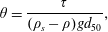 $$\begin{eqnarray}\unicode[STIX]{x1D703}=\frac{\unicode[STIX]{x1D70F}}{(\unicode[STIX]{x1D70C}_{s}-\unicode[STIX]{x1D70C})gd_{50}},\end{eqnarray}$$
where
 $\unicode[STIX]{x1D70F}$
is the bed shear stress,
 $\unicode[STIX]{x1D70C}_{s}$
the sediment density,
 $\unicode[STIX]{x1D70C}$
the water density,
 $g$
the gravity and
 $d_{50}$
the particle diameter. Shields (Reference Shields1936), and since many others, have determined that incipient motion, in the form of the rolling and/or sliding of a few grains at the surface of the bed, occurs for a critical
 $|\unicode[STIX]{x1D703}|$
in the range 0.03–0.05. The critical Shields criterion for threshold motion has been confirmed to be relevant for sediment motion under waves (e.g. Soulsby Reference Soulsby1997). However, this point of view assumes that the mechanisms for particle incipient motion for steady flows also apply to oscillatory flows. Madsen (Reference Madsen1974) and later Zala Flores & Sleath (Reference Zala Flores and Sleath1998) have at least identified that horizontal pressure flow induced gradients, not present in free-surface steady current flows, are potentially destabilizing even at subsediment-bed surface levels by exerting a horizontal seepage force on the sediment grains within the bed.
We therefore identify a number of challenges concerning incipient motion mechanisms. The first lies in the applicability of the bed failure concept in the case of free-surface waves. Although a certain number of tunnel flows in U-tube experiments (Dick & Sleath Reference Dick and Sleath1991; Zala Flores & Sleath Reference Zala Flores and Sleath1998) have shown that horizontal pressure gradients are capable of destabilizing granular layers, it has still to be understood how it extends to wave flow induced pressure gradients. To tackle this issue we face the fact that there is scarcely any comprehensive data sets available. This is certainly due to strong experimental difficulties in measuring simultaneously instantaneous pressure, velocities and moving interfaces in granular flows which in turn has of course strong implications on the estimation of the fluid shear stress exerted on the particles. The second complementary challenge concerns how this shear interplays with the other forces during bed failure mechanisms and what is the nature of the shear stress experienced by mobile layers of particles. Lastly, while in U-tubes pressure gradients are mainly in the flow direction, under waves vertical cross-wise pressure gradients extending from inside the bed to the free flow can also influence bed destabilization or favour mobile layer settling.
Madsen (Reference Madsen1974) was amongst the first to suggest that a momentary bed failure is likely to occur during the passage of the steep front slope of a near-breaking wave. This was inferred from measurements of horizontal pressure gradients under waves without sediment and a bed stability analysis by a geotechnical model. Bed failure refers to a situation in which the sediment bed at a certain level loses internal cohesion: it is a soil mechanics type of rupture. Horizontal fluid pressure gradients inside the bed trigger a horizontal seepage flow of Darcy type that results into a drag on each single particle and an overall body force inside the bed. The failure criterion involves the now so-called Sleath number, that is the ratio of the pressure induced horizontal destabilizing force to the stabilizing force applied by gravity
 $$\begin{eqnarray}S=\frac{\unicode[STIX]{x2202}p/\unicode[STIX]{x2202}x}{(\unicode[STIX]{x1D70C}_{s}-\unicode[STIX]{x1D70C})g},\end{eqnarray}$$
where
 $\unicode[STIX]{x2202}p/\unicode[STIX]{x2202}x$
is the horizontal pressure gradient. Unlike the Shields number, the Sleath number is independent of the particle size. Bed failure occurs if
 $$\begin{eqnarray}|S|\geqslant K_{f}\,C,\end{eqnarray}$$
where
 $K_{f}\,C$
is the threshold or critical value, with
 $K_{f}$
the internal friction angle and
 $C$
the sediment concentration. This criterion was later retrieved by Sleath (Reference Sleath1999). Madsen (Reference Madsen1974) also inferred from his geotechnical model and order of magnitude analysis that the failing/slipping layer would be approximately
 $10\,$
% of
 $H_{b}$
, where
 $H_{b}$
is the breaker wave height. Using lightweight particles as sediment and solitary free-surface wave forcing, Madsen & Durham (Reference Madsen and Durham2007) highlighted a somewhat different effect of horizontal pressure gradients in the form of deep cumulative particle displacements even though no bed failure was reached at any levels in the bed.
Bed failure induced sediment motion by a horizontal body force is in marked contrast with the shear induced incipient motion. In the latter case, the increasing shear stress applied by the wave at flow reversals on the surface of the sediment bed produces a layer by layer motion. The top layer of grains, set into motion by the flow, entrains the layer just below and so on down to the still bed where the granular shear is not sufficient to overcome the friction. This produces a sheared vertical velocity structure of the mobile granular layer (Aussillous et al.
Reference Aussillous, Chauchat, Pailha, Médale and Guazzelli2013). For the former case, the horizontal fluid pressure gradients inside the granular layer produce motions of thick layers of sediment called ‘plug flow’ in which the vertical velocity structure is uniform: the particles at all levels are moving at the same velocity, as clearly shown by Zala Flores & Sleath (Reference Zala Flores and Sleath1998). They obtained oscillatory plug flows in a U-tube set-up in which plastic particles start to move as a solid block of several diameters thick as flow reverses. This was indirectly evidenced experimentally with interstitial fluid velocity measurements. During plug flow the fluid is entrained by the particles and the fluid velocity is constant over a certain depth of the mobile layer. The first experimental evidence was in fact observed in the same U-tube by Dick & Sleath (Reference Dick and Sleath1991) with Sleath numbers as high as
 $0.92$
, as Sleath (Reference Sleath1999) later analysed.
Sleath (Reference Sleath1999) derived a destabilization model in which a block of sediment, with an upper boundary at the water/sediment interface, is about to slip if the horizontal pressure gradient exceeds friction forces due to weight of the block at the slip layer. This analysis is of course close to that of Madsen (Reference Madsen1974) and provides the same slip or failure criterion involving the Sleath number. This critical Sleath number is found to be approximately
 $0.35$
in the Zala Flores & Sleath (Reference Zala Flores and Sleath1998) experiments.
Foster et al. (Reference Foster, Bowen, Holman and Natoo2006) provides the first field evidence of incipient motion that is significantly influenced by the unsteady forcing introduced by the horizontal pressure gradient due to the free-stream velocity gradients in surface gravity waves. Sand buried hot-film sensors were able to record bed motion as deep as
 $2\,$
cm below the average bed interface position during the passage of wave fronts. A striking difference with U-tube (flow tunnel) measurements is that the critical Sleath number for plug flow initiation is found at a low value of
 $0.1$
which questions of course the previous investigations since
 $K_{f}\,C$
for loose random packing of granular materials varies approximately between
 $0.3$
and
 $0.4$
(Boyer, Guazzelli & Pouliquen Reference Boyer, Guazzelli and Pouliquen2011).
With regards to flow acceleration effects, the recent particle image velocimetry observations by Frank et al. (Reference Frank, Foster, Sou, Calantoni and Chou2015) in a U-tube experiment of the motion of an isolated protruding instrumented particle, show that incipient motion is strongly dependent on the streamwise pressure gradients of flows with large accelerations. The physical mechanisms by which the streamwise pressure gradient produces a force on the particle was not discussed but critical Sleath number for incipient motion computed from the macro scale flow parameters was approximately
 $0.1$
, in line with the previous findings by Foster et al. (Reference Foster, Bowen, Holman and Natoo2006). Observations in a flume by Terrile et al. (Reference Terrile, Reniers, Stive, Tromp and Verhagen2006) also discuss steep wave front acceleration effects on incipient motion of mono-layers of coarse particles. They observed gravel (
 $1$
cm diameter) moving for shear stresses well under Shields threshold value but large enough flow accelerations (approximately
 $1.8~\text{m}~\text{s}^{-2}$
). They qualitatively identified that flow acceleration increased the lift on particles favouring destabilization. These types of experiments even though exemplifying the role of pressure gradient are only loosely connected to the plug-type incipient motion discussed above because of the absence of seepage flows.
The Sleath (Reference Sleath1999) model assumes that when destabilization occurs, the block of sediment about to slip will move simultaneously upwards due to the dilation in the slip layer at the base of the block. Indeed the moving block particles have to free themselves from the interlocking with the underlying ones at rest. The pore volume increase induces a vertical inflow of fluid or equivalently a pressure drop in the bed. Sleath (Reference Sleath1999) claimed that this simultaneous pressure gradient produces a downwards vertical force acting as if the weight of the block is increased. Using the Darcy law, Sleath (Reference Sleath1999) estimated that this extra downwards pressure would shift the critical Sleath number to 0.75 in the case of a thick block (thick with respect to the particle diameter). This vertical seepage model however relies on two parameters difficult to measure or estimate: the dilatancy of the granular media and the time necessary for the block to break the interlocking. The value of 0.75 is associated with a very high value of the dilatancy only encountered in closed-packed centred body configuration, in other words for very compacted granular beds.
Besides this somewhat dubious mechanism, other vertical pressure gradient effects are also known to be important for bed destabilization and especially those leading to liquefaction (e.g. Yamamoto et al. Reference Yamamoto, Koning, Sellmeijer and van Hijum1978; Liu, Park & Lara Reference Liu, Park and Lara2007; Scholtès et al. Reference Scholtès, Chareyre, Michallet, Catalano and Marzougui2015). In the presence of free-surface waves, the vertical excess pore pressure gradients in the bed are the result of the delay in pressure transmission within the porous bed. Depending on the wave phase, these pressure gradients are expected to increase or decrease the apparent weight of the block, favouring motion or settling.
With the present understanding of plug flow initiation, pressure gradients both streamwise and vertically across the bed interface are paramount. Dick & Sleath (Reference Dick and Sleath1991) and others since, have traditionally used the external horizontal velocity time derivative for estimating streamwise pressure inside the sediment. Because of the phase lags of the horizontal fluid velocity along the vertical, of phase lag effects on the pressure transmission and pressure attenuation inside the bed (Yamamoto et al. Reference Yamamoto, Koning, Sellmeijer and van Hijum1978), the free-stream velocity derivative surrogate of horizontal pressure gradients should be handled with care. Pore pressure inside the sediment layer, be it moving or not, have been directly measured with arrays of pressure of small tappings closed with porous nylon filters and connected to pressure transducers (Sumer et al. Reference Sumer, Hatipoglu, Fredsøe and Sumer2006, Reference Sumer, Guner, Hansen, Fuhrman and Fredsøe2013). However this technique is mainly employed in sand or mud liquefaction studies.
The other experimental and instrumental issue in the understanding of incipient plug motion and dynamics, relates to the shear stress applied by the clear fluid flow above the sediment interface. The oscillating boundary layer at this interface is the place of highly fluctuating and strong gradients of fluid/grain velocities. Nowadays, velocity can be obtained with high resolution and accuracy with optical methods (Cowen et al. Reference Cowen, Dudley, Liao, Variano and Liu2010; van der A et al. Reference van der A, O’Donoghue, Davies and Ribberink2011; Rodríguez-Abudo, Foster & Henriquez Reference Rodríguez-Abudo, Foster and Henriquez2013; Henriquez et al. Reference Henriquez, Reniers, Ruessink and Stive2014) as long as particle concentration is low. Acoustics is certainly the best non-intrusive technique to date for high concentration laden flows, but is nonetheless questionable when approaching the still bottom roughness (Hay et al. Reference Hay, Zedel, Cheel and Dillon2012a ,Reference Hay, Zedel, Cheel and Dillon b ). This technique has proved its applicability for the understanding of oscillatory boundary layer dynamics on movable granular layers (Berni, Barthélemy & Michallet Reference Berni, Barthélemy and Michallet2013).
There is still an ongoing debate about the different methods for estimating the shear stress over rough beds (Sleath Reference Sleath1987; Yuan & Madsen Reference Yuan and Madsen2014). On one hand the ‘direct’ Reynolds method, by using Nielsen (Reference Nielsen1992) velocity decomposition for instance, might appear theoretically more sound compared to empirical law-of-the-wall log fit or integrated momentum budgets, but requires high time resolution measurements that capture turbulent velocity fluctuations down to very small scales, say of the order of a few grain sizes. On the other hand, direct measurements of local bed shear stress with a shear plate (Pujara & Liu Reference Pujara and Liu2014) or hot films (Sumer et al. Reference Sumer, Guner, Hansen, Fuhrman and Fredsøe2013) are not applicable for moving beds. To overcome such drawback, Sumer et al. (Reference Sumer, Guner, Hansen, Fuhrman and Fredsøe2013) combined sediment-bed experiments with the use of bed hot-film derived shear stresses measured in rigid-bed experiments. However the orbital vertical velocity component, associated with the bed vertical motion due to the erosion itself (Suarez et al. Reference Suarez, Barthelemy, Berni, Chauchat, Michallet and Cienfuegos2014), is obviously missed in such shear stress analysis. Significant phase-averaged vertical velocities in U-tube flows over rigid beds by van der A et al. (Reference van der A, O’Donoghue, Davies and Ribberink2011) are also detected near the bed throughout the flow cycle indicating that an additional shear stress, at least as large as the turbulent Reynolds stress, is to be taken into account.
Interface detection is not only important to validate velocity vertical structures (Berni et al. Reference Berni, Barthélemy and Michallet2013) but also to understand mobile layer thickness cycles (Zala Flores & Sleath Reference Zala Flores and Sleath1998). Conventional approaches are indirect interface detection through concentrations measurements (Sumer et al. Reference Sumer, Kozakiewicz, Fredsøe and Deigaard1996) by which interfaces are defined in terms of particle concentration. Recently Berni, Michallet & Barthélemy (Reference Berni, Michallet and Barthélemy2012) showed with wave basin experimental results that acoustic tracking of the dense granular flow layer enables elevation measurements of both the upper interface of the moving granular layer and of the still bed level, interface between the moving grains and the still ones. In the same effort Berni et al. (Reference Berni, Michallet and Barthélemy2012) qualitatively cross-validated the sheet flow layer motion with sand buried optical fibre motion detection.
In the present paper, a new set of experiments, carried out in a wave flume to understand pressure induced sediment motion, is presented. A combination of various probing techniques (acoustic sensors, optical fibres, pressure transducers) are deployed to understand pressure induced sediment-bed destabilization and the overall forces acting on the moving layer of the sediment bed. The paper is organized as follows. We first recall the plug model basics in § 2. The set-up of the experiments designed with lightweight sediment and the measuring devices are described in § 3. Section 4 is devoted to the evaluation of the shear stress induced by the wave flow on the sediment bed. Horizontal pressure gradient effects on plug flow initiation is the core of the paper and presented in § 5. Section 6 discusses how the vertical pressure gradients and the shear stress are expected to combine to facilitate or prevent plug flow. The main conclusions are drawn in the last section.
2 Sleath model of plug flow
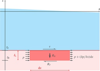
The conceptual model considered here was proposed by Sleath (Reference Sleath1994, Reference Sleath1999). It can be summarized as follows. The equilibrium of a moving volume of water–particle mixture of height
 $\unicode[STIX]{x1D6FF}_{s}$
and length
 $\text{d}x$
is considered, see figure 1. The flow above this block of sediment produces a shear stress
 $\unicode[STIX]{x1D70F}$
in the
 $x$
direction. The intergranular friction stress
 $R_{T}$
at the base of the slipping volume and the horizontal pore pressure gradient
 $\unicode[STIX]{x2202}p/\unicode[STIX]{x2202}x$
are the other external forces. The momentum balance equation for the plug in the
 $x$
direction reads
 $$\begin{eqnarray}\int _{z_{b}}^{z_{s}}\frac{\unicode[STIX]{x2202}(\unicode[STIX]{x1D70C}_{m}u)}{\unicode[STIX]{x2202}t}\,\text{d}z=-\unicode[STIX]{x1D6FF}_{s}\frac{\unicode[STIX]{x2202}p}{\unicode[STIX]{x2202}x}+\unicode[STIX]{x1D70F}+R_{T},\end{eqnarray}$$
where
 $\unicode[STIX]{x1D70C}_{m}=\unicode[STIX]{x1D70C}_{s}C+\unicode[STIX]{x1D70C}(C-1)$
is the density of the mixture of water and sediments making up the plug (
 $\unicode[STIX]{x1D70C}$
is the water density,
 $\unicode[STIX]{x1D70C}_{s}$
the sediment density and
 $C$
the volume concentration in sediment),
 $z_{b}$
and
 $z_{s}$
are respectively the bottom and the top of the plug.
Schematic diagram of the forces acting on a section of bed of height
 $\unicode[STIX]{x1D6FF}_{s}$
and length
 $\text{d}x$
: the effective weight
 $R_{N}$
, the shear stress of the flow
 $\unicode[STIX]{x1D70F}$
, the intergranular friction stress
 $R_{T}$
and the horizontal gradient of pore pressure
 $\unicode[STIX]{x2202}p/\unicode[STIX]{x2202}x$
. The waves propagate in the
 $x$
direction.
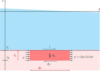
The horizontal velocity
 $u$
is assumed to be uniform within the plug and is noted
 $u_{s}$
, which leads to
 $$\begin{eqnarray}\unicode[STIX]{x1D70C}_{m}\unicode[STIX]{x1D6FF}_{s}\frac{\unicode[STIX]{x2202}u_{s}}{\unicode[STIX]{x2202}t}-\unicode[STIX]{x1D70C}_{m}u_{s}\frac{\unicode[STIX]{x2202}\unicode[STIX]{x1D6FF}_{s}}{\unicode[STIX]{x2202}t}=-\unicode[STIX]{x1D6FF}_{s}\frac{\unicode[STIX]{x2202}p}{\unicode[STIX]{x2202}x}+\unicode[STIX]{x1D70F}+R_{T}.\end{eqnarray}$$
Note that (2.2) holds if the variations of
 $\unicode[STIX]{x1D70C}_{m}$
are small with respect to that of
 $u$
.
The vertical component
 $R_{N}$
of stress carried by grain/grain interactions at the lower surface of the bed portion is the resultant of the sediment weight and a vertical pore pressure difference:
 $$\begin{eqnarray}\displaystyle R_{N} & = & \displaystyle \left[C\unicode[STIX]{x1D70C}_{s}+(1-C)\unicode[STIX]{x1D70C}\right]g\;\unicode[STIX]{x1D6FF}_{s}+p(z=z_{s})-p(z=z_{b})\nonumber\\ \displaystyle & = & \displaystyle \unicode[STIX]{x1D6FF}_{s}\left[C\,(\unicode[STIX]{x1D70C}_{s}-\unicode[STIX]{x1D70C})g+p_{z}^{\ast }\right],\end{eqnarray}$$
where
 $$\begin{eqnarray}p_{z}^{\ast }=\frac{p(z=z_{s})-p(z=z_{b})}{\unicode[STIX]{x1D6FF}_{s}}+\unicode[STIX]{x1D70C}g\end{eqnarray}$$
is the excess pore pressure gradient. Assuming Coulomb’s law (Bagnold Reference Bagnold1956), the dispersive stress or intergranular friction
 $R_{T}$
when the plug is set into motion can be expressed as:
 $$\begin{eqnarray}\displaystyle R_{T} & = & \displaystyle -\text{sign}(u_{s})\;K_{f}\;R_{N}\nonumber\\ \displaystyle & = & \displaystyle -\text{sign}(u_{s})\;K_{f}\;\left[C(\unicode[STIX]{x1D70C}_{s}-\unicode[STIX]{x1D70C})g+p_{z}^{\ast }\right]\;\unicode[STIX]{x1D6FF}_{s},\end{eqnarray}$$
where
 $K_{f}$
is the friction coefficient, equal to the tangent of the internal friction angle. It should be noted that this equation only holds for
 $R_{N}>0$
. The case
 $R_{N}<0$
gives a criterion for bed destabilization by liquefaction, in other words the conditions for which intergranular contacts cease (e.g. Scholtès et al.
Reference Scholtès, Chareyre, Michallet, Catalano and Marzougui2015). Substituting (2.5) into (2.2), the horizontal equation of motion of the plug reads:
 $$\begin{eqnarray}\unicode[STIX]{x1D70C}_{m}\unicode[STIX]{x1D6FF}_{s}\hspace{2.22198pt}\frac{\unicode[STIX]{x2202}u_{s}}{\unicode[STIX]{x2202}t}-\unicode[STIX]{x1D70C}_{m}u_{s}\frac{\unicode[STIX]{x2202}\unicode[STIX]{x1D6FF}_{s}}{\unicode[STIX]{x2202}t}=-\unicode[STIX]{x1D6FF}_{s}\frac{\unicode[STIX]{x2202}p}{\unicode[STIX]{x2202}x}+\unicode[STIX]{x1D70F}-\text{sign}(u_{s})\;K_{f}\left[C(\unicode[STIX]{x1D70C}_{s}-\unicode[STIX]{x1D70C})g+p_{z}^{\ast }\right]\unicode[STIX]{x1D6FF}_{s},\end{eqnarray}$$
considering that the intergranular friction force is exerted in the opposite direction to that of the plug velocity
 $u_{s}$
. At this stage no assumptions are formulated on the origin of the vertical excess pore pressure gradients. This will be discussed in § 6. Some of the terms in (2.6) can be challenging to determine experimentally, as will be discussed in § 6. Noteworthy is the semi-analytical model proposed by Lanckriet & Puleo (Reference Lanckriet and Puleo2015) for the computation of sheet flow thicknesses. It is based on similar ingredients as Sleath’s (1999) analytical model and shows good agreement with measurements performed in U-tubes.
Assuming the vertical pressure gradient is neglected:
 $$\begin{eqnarray}p_{z}^{\ast }\ll C(\unicode[STIX]{x1D70C}_{s}-\unicode[STIX]{x1D70C})g,\end{eqnarray}$$
the critical condition for sediment to start moving as a block can then be written as:
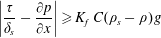 $$\begin{eqnarray}\left|\frac{\unicode[STIX]{x1D70F}}{\unicode[STIX]{x1D6FF}_{s}}-\frac{\unicode[STIX]{x2202}p}{\unicode[STIX]{x2202}x}\right|\geqslant K_{f}\hspace{2.22198pt}C(\unicode[STIX]{x1D70C}_{s}-\unicode[STIX]{x1D70C})g\end{eqnarray}$$
or as:
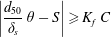 $$\begin{eqnarray}\left|\frac{d_{50}}{\unicode[STIX]{x1D6FF}_{s}}\hspace{2.22198pt}\unicode[STIX]{x1D703}-S\right|\geqslant K_{f}\hspace{2.22198pt}C\end{eqnarray}$$
with two dimensionless numbers, namely the Shields number
 $\unicode[STIX]{x1D703}$
(1.1) and the Sleath number
 $S$
(1.2). Special attention is devoted in the present study to the case of a thick destabilization depth, that is
 $d_{50}/\unicode[STIX]{x1D6FF}_{s}\ll 1$
, for which equation (2.9) yields
 $$\begin{eqnarray}\left|S\right|\geqslant K_{f}\hspace{2.22198pt}C.\end{eqnarray}$$
Another limiting case of interest is that of a flow with zero pressure gradient (
 $S=0$
) mobilizing, by applied surface shear, a top layer of one particle diameter thick (
 $\unicode[STIX]{x1D6FF}_{s}=d_{50}$
):
 $$\begin{eqnarray}\left|\unicode[STIX]{x1D703}\right|\geqslant K_{f}\hspace{2.22198pt}C.\end{eqnarray}$$
This can be interpreted as the lower bound of the Shields number for sheet flow transport, which is of course expected to be larger than the threshold for particle incipient motion in the bed load regime. In the framework of turbulent flows, this is in accordance with the study of Lajeunesse, Malverti & Charru (Reference Lajeunesse, Malverti and Charru2010). Extrapolation of their experimental results to a non-dimensional surface density of moving particles of
 $1$
(a moving top grain for each underlying grain) yields a Shields number of approximately
 $0.26$
.
3 Experimental set-up
3.1 Wave flume and flow conditions
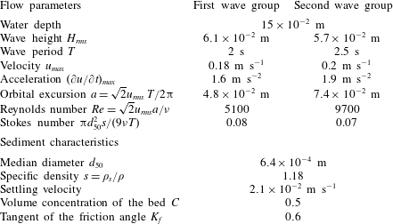
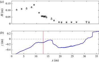
The laboratory experiments took place in a 36 m long and 0.55 m wide wave flume equipped with a piston wave generator (see figure 2). This facility is used to mimic natural beach dynamics with a length scaling of
 $1/10$
and a time scaling of approximately
 $1/3$
. The mobile bed consists of low density (
 $\unicode[STIX]{x1D70C}_{s}=1.18~\text{g}~\text{cm}^{-3}$
) polymethyl methacrylate (pmma) angular-shaped coarse grains (
 $d_{50}=640~\unicode[STIX]{x03BC}\text{m}$
, see the size distribution in Grasso, Michallet & Barthélemy Reference Grasso, Michallet and Barthélemy2011a
). This particular sediment was selected to fulfil a Shields number and Rouse number scaling (Grasso et al.
Reference Grasso, Michallet, Barthélemy and Certain2009; Berni et al.
Reference Berni, Barthélemy and Michallet2013). The water depth at the wave maker is 0.553 m. The sediment bed covers most of the flume (from
 $x=1.6~\text{m}$
to 36 m). The wave forcing is a sequence composed of two bichromatic wave groups of frequencies (0.478 Hz, 0.523 Hz) and (0.378 Hz, 0.422 Hz) separated by a rest period of 5 s, so to produce two distinct wave packets of 10 and 8 waves, with carrier wave periods of 2 s and 2.5 s, respectively. The significant wave height is set to 0.16 m at the wave maker for both groups. The duration of the wave sequence is
 $T_{s}=53.5~\text{s}$
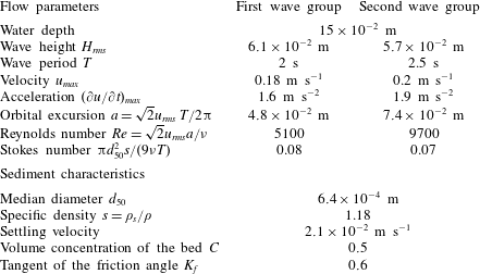
. It can be repeated continuously as much as desired. The different experimental parameters are summarized in table 1. The friction factor is estimated from the angle of repose of a sediment pile, so that
 $K_{f}=0.6\pm 0.03$
. The bed porosity is estimated through sediment settling in a graduated cylinder full of water. The sediment concentration of deposited beds is
 $C=0.5\pm 0.02$
. The product
 $K_{f}\hspace{2.22198pt}C$
is noteworthy equal to
 $0.3$
. Indeed Boyer et al. (Reference Boyer, Guazzelli and Pouliquen2011) studied the rheology of granular sheared media for large ranges of shear and particle concentrations all leading to a similar estimate (
 $\unicode[STIX]{x1D707}\hspace{2.22198pt}\unicode[STIX]{x1D719}\simeq 0.3$
with their notations) to what could be a general value of
 $K_{f}\,C$
.
The choice of the wave conditions is based on previous laboratory experiments of intermediate cross-shore barred-beach morphodynamics in the same flume (Grasso, Michallet & Barthélemy Reference Grasso, Michallet and Barthélemy2011b
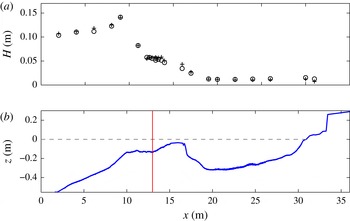
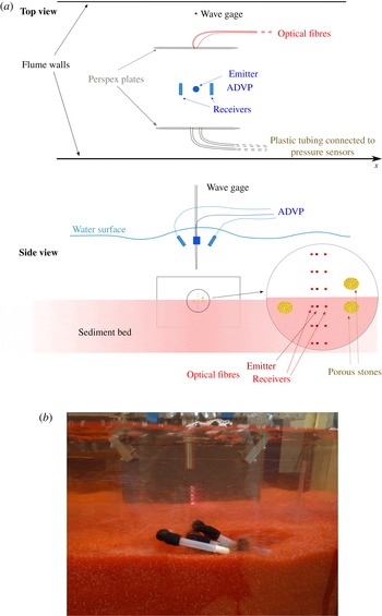
; Prel, Michallet & Barthélemy Reference Prel, Michallet and Barthélemy2011). This choice is made in order to minimize changes in the beach mean profile over the duration of the experiment, in particular at the location of interest in the surf zone. The corresponding barred-beach profile is presented in figure 2. Capacitive wave gages are placed in the cross-shore direction of the beach to measure free-surface elevations. The root mean square wave height
 $H_{rms}$
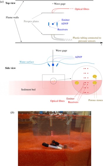
variation with the cross-shore position is also plotted. The main measurement location is in the surf zone, where several devices were deployed as schematized in figure 3: pressure sensors, optical sensors and an acoustic velocity profiler, that are described in more detail in the following.
Summary of experimental parameters at the measurement location.
(a) Root mean square wave height (pluses:
 $T=2~\text{s}$
; circles:
 $T=2.5~\text{s}$
) along (b) the beach topography:
 $x=0$
is the mean position of the wave maker,
 $z=0$
is the still free surface (horizontal dashed line). The thin vertical line indicates the measurement location (
 $x=13~\text{m}$
).
(a) Schematic diagram and (b) side view picture of the instrumental set-up. The tips of the optical and pressure elements were fixed into Perspex plates 30 cm long and 20 cm high.
3.2 Acoustic measurements
An acoustic Doppler velocity profiler (ADVP) was deployed (i) to profile the velocity field in the near-bed region and (ii) to measure at high frequency the elevations of both the still bed and the top of the moving sediment layer. A detailed description of the instrument principles and performances is provided in Hurther (Reference Hurther2001) and Bricault (Reference Bricault2006). Measurements in laboratory flows over dunes and in a natural surf zone were performed by Mignot et al. (Reference Mignot, Hurther, Chassagneux and Barnoud2009) and Hurther & Thorne (Reference Hurther and Thorne2011), it was further used for tracking the bed mobility in oscillatory boundary layers by Ruessink et al. (Reference Ruessink, Michallet, Abreu, Sancho, Van der A, Van der Werf and Silva2011) and Berni et al. (Reference Berni, Michallet and Barthélemy2012). The principle of velocity measurements is briefly recalled here, the method for bed height detection is presented in more detail and justified in appendix A.
The ADVP emits ultrasonic pulses in the form of wave trains of frequency
 $f_{0}=1~\text{MHz}$
in the vertical direction downwards. The pulse repetition frequency (
 $f_{r}$
) is 1600 Hz. This acoustic wave is scattered by both solid particles and air micro-bubbles. Two receivers oriented streamwise detect the back-scattered acoustic wave trains. The received signal is binned into time intervals of
 $4~\unicode[STIX]{x03BC}\text{s}$
called gates. Each gate corresponds to a sampling volume at a specific distance of the emitting ceramic.
The velocity components along each beam axis are estimated from a Doppler frequency shift detection. Knowing the exact geometrical configuration of the emitter and the receivers, the horizontal and vertical velocities are then computed using a geometrical transformation.
Instantaneous horizontal
 $u$
and vertical
 $w$
velocity components are measured at a sampling rate of 50 Hz along a vertical profile of about 5 cm above the bed with a typical distance between each measurement volume of
 $3~\text{mm}$
. This signal is obtained for a time interval covering a large number of sequences, the phase-averaged velocity
 $\widetilde{u}$
can be therefore computed as:
 $$\begin{eqnarray}\widetilde{u}(z,t)=\frac{1}{N}\mathop{\sum }_{n=1}^{N}u(z,t+(n-1)\;T_{s}),\end{eqnarray}$$
where
 $N$
is the number of (
 $T_{s}=53.5~\text{s}$
)-sequences and
 $u(z,t)$
is the instantaneous signal at elevation
 $z$
. The near-bed velocity (
 $u_{0}$
) is measured at an elevation
 $z=z_{0}$
, corresponding to the first measurement volume above the still bed height (
 $z_{b}$
) measured as explained in the Appendix. It has been checked that the results presented hereafter are not very sensitive to this definition: choosing a gate just above
 $z_{0}$
does not change the conclusions drawn in this paper. The free-stream velocity
 $u_{\infty }$
is measured at a fixed elevation above the boundary layer, that is at about 2 cm above the still bed.
3.3 Optical fibre sensors
An array of optical sensors is deployed in the flume to detect the bed incipient motion and mobility. Each optical fibre sensor is composed of three fibres: an emitter and two receivers. The emission is a discontinuous optical signal switched alternatively on and off at
 $500$
Hz. The surrounding light is received when the emission is off and the corresponding voltage can be subtracted from the total signal recorded when the emission is on. Thus the resulting signal for each reception fibre only corresponds to the light scattered by the sediments. The sampling volume is only of a few mm
 $^{3}$
and the sampling frequency of
 $50\,$
Hz.
The bed stability is characterized by the time derivative of the signal (Berni et al.
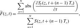
Reference Berni, Mignot, Michallet, Dalla-Costa, Grasso and Lagauzère2009): large variations mean that the sediment is moving. The fluctuation of the signal of the optical sensors is quantified by an ensemble average
 $\widetilde{F}$
defined as:
 $$\begin{eqnarray}\widetilde{F}(z,t)=\frac{\displaystyle \mathop{\sum }_{n=1}^{N}\text{abs}\left({\displaystyle \frac{\unicode[STIX]{x2202}S_{f}(z,t+(n-1)\;T_{s})}{\unicode[STIX]{x2202}t}}\right)}{\displaystyle \mathop{\sum }_{n=1}^{N}S(z,t+(n-1)\;T_{s})},\end{eqnarray}$$
where
 $N$
is the number of sequences,
 $S_{f}(z,t)$
the instantaneous voltage signal at the elevation
 $z$
. Bed is considered at rest when
 $\widetilde{F}<0.6~\text{s}^{-1}$
. This threshold value was obtained from the mean and the standard deviation of measurements within a bed at rest.
Ensemble-averaged ADVP interface and optical fibre measurements are cross-analysed for
 $N=92$
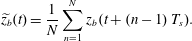
repetitions of the wave sequence. The ensemble-averaged bed elevation is computed from the instantaneous bed elevation (
 $z_{b}$
, see the Appendix) as:
 $$\begin{eqnarray}\widetilde{z_{b}}(t)=\frac{1}{N}\mathop{\sum }_{n=1}^{N}z_{b}(t+(n-1)\;T_{s}).\end{eqnarray}$$
The top of the mobile layer
 $z_{s}$
is phase-averaged similarly. The position of the two interfaces
 $\widetilde{z_{b}}$
and
 $\widetilde{z_{s}}$
along with the fluctuating signal
 $\widetilde{F}$
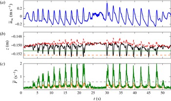
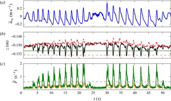
at two specific elevations are plotted in figure 4. Every time the bed interface
 $z_{b}$
crosses the fibre sensor elevation, the fibre sensor fluctuating signal exceeds the particle motion threshold value. This comparison clearly indicates that the interface detection with the acoustics is reliable both in time and elevations.
Time series of (a) the free-stream velocity
 $\widetilde{u}_{\infty }$
, (b) the position of interfaces (bed:
 $\widetilde{z}_{b}$
, black solid line and top of the mobile sediment layer:
 $\widetilde{z}_{s}$
, red dashed line,
 $z=0$
corresponds to the still water free surface) and (c) the signal of two optical sensors
 $\widetilde{F}$
(solid and dashed lines) at the positions marked with horizontal lines in the middle panel (solid and dashed lines, respectively). The horizontal dashed line in (c) is the threshold value above which bed particles are deemed to move.
3.4 Pressure measurements
Three pressure sensors (STS®ATM/N, with manufacturer’s specified time response of 1 ms) were installed at the same position
 $x=13~\text{m}$
as for both the fibre sensors and the ADVP, in order to estimate the vertical and horizontal pressure gradients. The tip of a 5 mm rigid tube which is located at the measuring point is equipped with a porous stone. The other end of the tube is connected to the pressure sensor remotely placed deep into the bed. The pressure range for these sensors is between 0 and 100 mbar with an accuracy of 0.1 mbar. The distance between the sensors aligned vertically was
 $1.2$
cm. The distance between the two sensors aligned horizontally was
 $d=3$
cm. As this distance is small compared to the wavelength, the pressure gradient can be computed precisely as:
 $$\begin{eqnarray}\frac{\unicode[STIX]{x2202}p}{\unicode[STIX]{x2202}x}=\frac{\unicode[STIX]{x0394}p}{d},\end{eqnarray}$$
where
 $\unicode[STIX]{x0394}p$
is the pressure difference between these two sensors. The second-order error introduced by using (3.4) is of the order of:
 $$\begin{eqnarray}\frac{\unicode[STIX]{x2202}^{2}p}{\unicode[STIX]{x2202}x^{2}}\times \frac{d}{2},\end{eqnarray}$$
where the second derivative can be estimated as
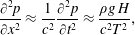 $$\begin{eqnarray}\frac{\unicode[STIX]{x2202}^{2}p}{\unicode[STIX]{x2202}x^{2}}\approx \frac{1}{c^{2}}\frac{\unicode[STIX]{x2202}^{2}p}{\unicode[STIX]{x2202}t^{2}}\approx \frac{\unicode[STIX]{x1D70C}g\,H}{c^{2}T^{2}},\end{eqnarray}$$
while the first-order derivative can be evaluated as
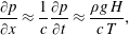 $$\begin{eqnarray}\frac{\unicode[STIX]{x2202}p}{\unicode[STIX]{x2202}x}\approx \frac{1}{c}\frac{\unicode[STIX]{x2202}p}{\unicode[STIX]{x2202}t}\approx \frac{\unicode[STIX]{x1D70C}g\,H}{c\,T},\end{eqnarray}$$
where
 $c$
is the wave celerity,
 $H$
the wave height and
 $T$
the period. For a wave with a wave height of 6 cm, a period of 2.5 s, a water depth
 $h$
of 15 cm, and with the approximation
 $c=\sqrt{gh}$
, the relative error is:
 $$\begin{eqnarray}\left.\frac{\unicode[STIX]{x2202}^{2}p}{\unicode[STIX]{x2202}x^{2}}\times \frac{d}{2}/\frac{\unicode[STIX]{x2202}p}{\unicode[STIX]{x2202}x}\right.\approx \frac{d}{2~c\,T}\sim 5\times 10^{-3}.\end{eqnarray}$$
In the framework of the linear wave theory, this horizontal pressure gradient within the boundary layer above the bed is known to be proportional to the free-stream acceleration of the flow (Nielsen Reference Nielsen1992):
 $$\begin{eqnarray}\frac{\unicode[STIX]{x2202}u_{\infty }}{\unicode[STIX]{x2202}t}=-\frac{1}{\unicode[STIX]{x1D70C}}\frac{\unicode[STIX]{x2202}p}{\unicode[STIX]{x2202}x}.\end{eqnarray}$$
Obviously (3.9) also holds for ensemble-averaged values:
 $$\begin{eqnarray}\frac{\unicode[STIX]{x2202}\widetilde{u}_{\infty }}{\unicode[STIX]{x2202}t}=-\frac{1}{\unicode[STIX]{x1D70C}}\frac{\unicode[STIX]{x2202}\widetilde{p}}{\unicode[STIX]{x2202}x}.\end{eqnarray}$$
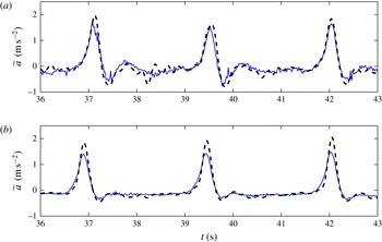
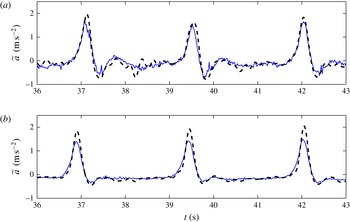
Horizontal pressure gradients measured at two different elevations inside the bed are presented and compared to flow accelerations in figure 5. Note that the accelerations in figure 5(a,b) cannot be directly compared as the experiment presented in figure 5(a) was performed over a beach profile slightly different from the one presented in figure 2. However in both cases the measurements of our experiments agree closely to relation (3.10) even though the sensors are below the bed interface. We have an indication that while the flow is oscillatory the pressure fluctuations within the few centimetres below the bed interface replicate the pressure fluctuations above the bed. Near the bed interface, there is a very good agreement between both measurements. Deeper inside the bed, the pressure gradient peaks are smaller than that of the free-stream acceleration as the pressure is slightly attenuated. Of note, the deceleration after the peaks can produce strong adverse pressure negative gradients close to the bed interface.
Comparison between free-stream acceleration of the flow
 $\unicode[STIX]{x2202}\widetilde{u_{\infty }}/\unicode[STIX]{x2202}t$
(dashed line) and
 $-1/\unicode[STIX]{x1D70C}~\unicode[STIX]{x2202}\widetilde{p}/\unicode[STIX]{x2202}x$
(thin solid line) for two different experiments, with the pressure sensors located 1 cm (a) and 6 cm (b) below the initial still bed level.
4 Bed shear stress estimation
Turbulence and orbital motion contributions to the shear stress are analysed in this section. To this end, the flow characteristics in terms of turbulence spectrum, intensities and orbital motions are detailed.
Because the fluid flow is the addition of wave, mean and turbulent motions, a traditional Reynolds decomposition is inadequate to obtain the fluctuating turbulent fluid velocities. Here we use a standard method (e.g. Hussain & Reynolds Reference Hussain and Reynolds1970), since the fluid velocity can be decomposed as
 $$\begin{eqnarray}u=\widetilde{u}+u^{\prime },\end{eqnarray}$$
where
 $\widetilde{u}$
is the ensemble average as defined by (3.1). However this method is not applicable to experiments over a mobile bed whose profile is evolving, since velocity variability at the time scale of the profile slow evolutions would contribute to the turbulence. To overcome this drawback, specific experiments with minimal bed changes were analysed in order to compute realistic turbulent shear stresses. The still bed position was detected using the ADVP, as described above. The near-bed velocity is defined as the velocity measured at the first measurement volume (at
 $z=z_{0}$
) above the still bed height position (
 $z_{b}$
). We selected
 $92$
repetitions of the sequence for which the bed level at the start of each repetition remained constant within a
 $\pm 1.5\;$
mm error bound. The root mean square (rms) turbulent fluctuation, or turbulence intensity, is computed as:
 $$\begin{eqnarray}u_{rms}^{\prime }(t,z)=\left[\frac{1}{N}\mathop{\sum }_{n=1}^{N}\left(u(t+(n-1)\;T_{s},z)-\widetilde{u}(t,z)\right)^{2}\right]^{1/2}.\end{eqnarray}$$
The same type of relation is used for the vertical velocity to define the turbulence vertical intensity
 $w_{rms}^{\prime }$
. The Reynolds stress is computed as
 $$\begin{eqnarray}-\unicode[STIX]{x1D70C}\widetilde{u^{\prime }w^{\prime }}(t,z)=\frac{1}{N}\mathop{\sum }_{n=1}^{N}\left(u(t+(n-1)\;T_{s},z)-\widetilde{u}(t,z)\right)\left(w(t+(n-1)\;T_{s},z)-\widetilde{w}(t,z)\right).\end{eqnarray}$$
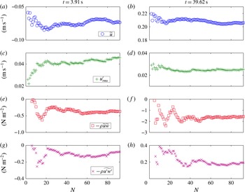
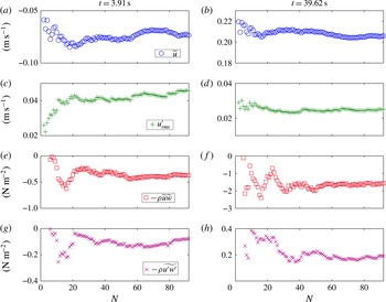
To check the number of realizations required for the statistical moments of the turbulence to converge, we computed the ensemble-averaged velocity (3.1), the standard deviation of the horizontal fluctuations (4.2) and two components of the bed shear stress for
 $N$
varying between
 $1$
and
 $92$
. Some results are plotted in figure 6 for selected phases (one wave trough and one wave crest) and measurements at
 $z=z_{0}$
. Because the bed level is slightly different for each sequence, rather large variations of the estimators are obtained for small values of
 $N$
. It appears that
 $N=40$
realizations are sufficient for the statistical estimators to converge with a relatively good accuracy.
Convergence, with the number of wave sequences, of (from top to bottom) the orbital horizontal velocity, the rms turbulent fluctuation, the orbital component of the shear stress and the Reynolds stress, at
 $z=z_{0}$
, at the phase of one typical wave trough (a,c,e,g) and at the phase of one typical wave crest (b,d,f,h).
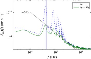
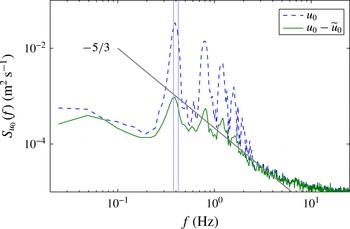
The spectra of both the turbulent and ensemble-averaged near-bed horizontal velocities are given in figure 7. These spectra are computed for the bichromatic wave group of carrier period 2.5 s. Up to about 5 Hz, the turbulent horizontal velocity spectrum exhibits a trend that approximately follows a
 $-5/3$
slope, as would be expected. The ensemble-average horizontal velocity spectrum is characterized by peak at approximately 0.4 Hz corresponding to the pair of frequencies related to the two frequency components of the bichromatic wave packet. The peaks at higher frequencies correspond to harmonics of these two basic frequencies. The large amount of super-harmonics is an indication of the high degree of wave nonlinearity (departure from linear wave theory) in the surf zone.
Power spectral density of the near-bed horizontal velocity (dashed line) and its turbulent component (solid line). The grey line marks a
 $-5/3$
slope. The vertical lines correspond to the 2 frequencies making up the bichromatic wave group.
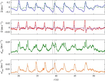
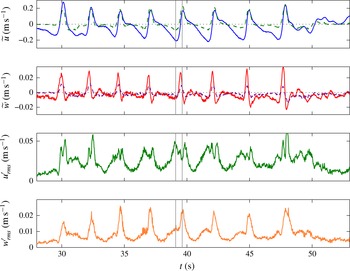
The near-bed turbulence intensities are displayed in figure 8 along with the ensemble-averaged horizontal and vertical velocities measured outside the boundary layer and near the bed. The vertical ensemble-averaged velocities show large peaks at phases of large horizontal flow acceleration corresponding to the steep wave fronts.
The horizontal turbulence intensity is five times smaller than the free-stream orbital velocity, slightly larger than in previous laboratory experiments (e.g. Chen et al.
Reference Chen, Chen, Tang, Stansby and Li2007; van der A et al.
Reference van der A, O’Donoghue, Davies and Ribberink2011). The vertical turbulence intensity is two times smaller than the horizontal turbulence intensity, in agreement with previous laboratory experiments (Sleath Reference Sleath1987; Jensen, Sumer & Fredsøe Reference Jensen, Sumer and Fredsøe1989; Chen et al.
Reference Chen, Chen, Tang, Stansby and Li2007; van der A et al.
Reference van der A, O’Donoghue, Davies and Ribberink2011). The vertical turbulence intensity,
 $w_{rms}^{\prime }$
, is maximum under the crest and the trough. As shown by van der A et al. (Reference van der A, O’Donoghue, Davies and Ribberink2011) for asymmetric waves, the horizontal turbulence intensity is larger under the crest than under the trough. This difference is more pronounced since the wave velocity asymmetry in our experiments, induced by steep wave fronts, is larger than in the U-tube experiments of van der A et al. (Reference van der A, O’Donoghue, Davies and Ribberink2011). Accordingly, the values at both flow reversals also known as zero crossing, are different. The vertical turbulence intensity is larger at the zero up-crossing flow reversal than it is at the zero down-crossing. The same trend can be observed for the horizontal turbulence intensity
 $u_{rms}^{\prime }$
, except that it sharply drops under the crest. These drops in the horizontal intensity occur simultaneously with peaks in the vertical intensity and correspond to specific moments of plug flow development as will be shown later.
Time series of orbital velocities
 $\widetilde{u}$
,
 $\widetilde{w}$
(solid line: free stream, dashed line: near bed) and the near-bed turbulence intensities
 $u_{rms}^{\prime }\,(z=z_{0})$
,
 $w_{rms}^{\prime }\,(z=z_{0})$
. Vertical lines indicate the phases of one trough and one crest.
Following Nielsen (Reference Nielsen1992), the shear stress is split into three contributions as
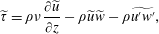 $$\begin{eqnarray}\displaystyle \widetilde{\unicode[STIX]{x1D70F}}=\unicode[STIX]{x1D70C}\unicode[STIX]{x1D708}\frac{\unicode[STIX]{x2202}\widetilde{u}}{\unicode[STIX]{x2202}z}-\unicode[STIX]{x1D70C}\widetilde{u}\widetilde{w}-\unicode[STIX]{x1D70C}\widetilde{u^{\prime }w^{\prime }}, & & \displaystyle\end{eqnarray}$$
where
 $\unicode[STIX]{x1D70C}\unicode[STIX]{x1D708}(\unicode[STIX]{x2202}\widetilde{u}/\unicode[STIX]{x2202}z)$
is the viscous induced momentum diffusion term,
 $-\unicode[STIX]{x1D70C}\widetilde{u}\widetilde{w}$
the orbital velocity induced momentum diffusion term and
 $-\unicode[STIX]{x1D70C}\widetilde{u^{\prime }w^{\prime }}$
the turbulence induced momentum diffusion term, the so-called Reynolds shear stress.
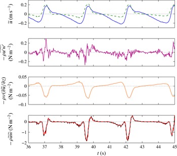
The bed shear stress is estimated with (4.4) at an elevation
 $z_{0}$
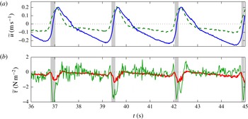
as close to the bed as possible (i.e. between 0 and 3 mm above the still bed elevation). The three terms of (4.4) are compared in figure 9 which clearly shows that the orbital term prevails in order of magnitude. The viscous term and the Reynolds shear stress are at most phases less than 10 % of the total stress, which is consistent with previous results on mobile beds (see Rodríguez-Abudo & Foster (Reference Rodríguez-Abudo and Foster2014), for instance). Despite the noise, the Reynolds shear stress estimates are consistent with previous observations of van der A et al. (Reference van der A, O’Donoghue, Davies and Ribberink2011) for example, with a time evolution phased with the free-stream horizontal velocity.
Time series of the free-stream (solid) and near-bed (dashed) velocities and the three contributions to the shear stress (4.4) estimated at
 $z=z_{0}$
. In the bottom plot, both the orbital component (solid) and the total shear stress (dashed) are plotted.
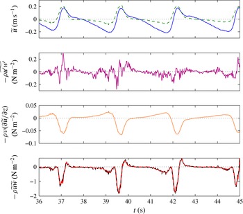
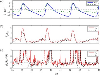
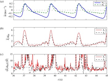
The most striking result is that the shear stress is negative at phases of large positive near-bed velocities. This will be further discussed in the next sections. At this stage, additional remarks can be made. The dimensionless mobile layer thickness and erosion depth are plotted in figure 10. Here the erosion depth is estimated with respect to the maximum bed elevation within each wave cycle. As shown in figure 10(b), both the erosion depth and the mobile layer thickness become greater than one grain size at wave troughs, and reach larger values below wave crests. Due to the relative magnitudes of
 $\widetilde{\unicode[STIX]{x1D6FF}_{e}}$
and
 $\widetilde{\unicode[STIX]{x1D6FF}_{s}}$
, it is noteworthy that the mobile layer concentration is likely to be approximately 25 % less than the assumed value
 $C=0.5$
at some phases. The detected bed evolution is plotted against the dimensionless shear stress in figure 10(c). Below the wave troughs,
 $\widetilde{\unicode[STIX]{x1D6FF}}/d_{50}/|\widetilde{\unicode[STIX]{x1D703}}|\simeq 5$
, which lies in the range 3–10 of previous shear stress driven sheet flow measurements (Wilson Reference Wilson1987; Sumer et al.
Reference Sumer, Kozakiewicz, Fredsøe and Deigaard1996; Zala Flores & Sleath Reference Zala Flores and Sleath1998; O’Donoghue & Wright Reference O’Donoghue and Wright2004). The largest values of this ratio exceed 10 and are reached at flow reversals from trough to crest, and behind the wave crests. These high values of
 $\unicode[STIX]{x1D6FF}_{e}$
or
 $\unicode[STIX]{x1D6FF}_{s}$
that are beyond the sheet flow regime seem to indicate that driving effects other than the shear stress might prevail.
Time series of (a) the free-stream horizontal velocity
 $\widetilde{u}_{\infty }$
and the near-bed velocity
 $u_{0}$
, (b) the dimensionless mobile layer thickness
 $\widetilde{\unicode[STIX]{x1D6FF}}_{s}/d_{50}$
and erosion depth
 $\widetilde{\unicode[STIX]{x1D6FF}}_{e}/d_{50}$
and (c) the ratio of the dimensionless thickness to the dimensionless shear stress.
5 Horizontal pressure gradient effects on bed incipient motion
In previous sections, oscillatory flow induced horizontal pressure gradients were described as a potential body force for bed destabilization (§ 2) but also measured and shown to be in agreement with the flow accelerations (see figure 5). In the present section we evaluate and describe how this body force explains part of the mobile layer motion inception.
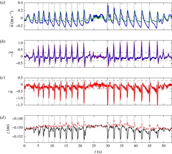
Time series of horizontal velocities (solid: free-stream velocity, dashed: near-bed velocity); opposite of the Sleath computed with the pressure gradient (thick line) or the acceleration of the flow (thin line); Shields number; positions of the bed (
 $\widetilde{z_{b}}$
, solid line) and the top of the mobile layer (
 $\widetilde{z_{s}}$
, dashed line) interfaces. The grey stripes correspond to time intervals where an erosion rate
 $-\unicode[STIX]{x2202}\widetilde{z_{b}}/\unicode[STIX]{x2202}t$
greater than
 $6~\text{mm}~\text{s}^{-1}$
is detected. The horizontal dashed lines in (b) and (c) mark the
 $K_{f}C$
threshold.
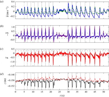
Close-up of figure 11, second bichromatic wave group,
 $T=2.5~\text{s}$
.
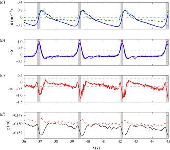
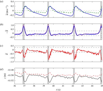
The overall flow characteristics of a selected experiment are displayed in figure 11 for the entire wave sequence and in figure 12 for only three waves of the second bichromatic wave group. Time series of the near-bed and the free-stream horizontal orbital velocities are presented along with the elevation of the still bed
 $\widetilde{z_{b}}$
and the elevation of the top of the mobile layer
 $\widetilde{z_{s}}$
. As discussed in Berni et al. (Reference Berni, Barthélemy and Michallet2013), the free-stream horizontal velocity is seen to be asymmetric, especially in the second wave group whereas the near-bed velocity is skewed. Free-stream velocity asymmetry induces skewed accelerations that in turn generate skewed horizontal pressure gradients (figure 5). Additionally a mobile layer develops under each wave crests, corresponding to a strong and rapid erosion of the bed but also to an increase in the elevation of the top of the mobile layer, as clearly seen in figure 12. The mobile layer thickness can reach values up to 4 mm. The mobile layer variation is also strongly asymmetric in time, suggesting that pressure gradients are favourable to mobile layer development.
On one hand bed plug formation by pressure gradients should occur if the Sleath number
 $|S|$
exceeds the threshold value
 $K_{f}\,C$
(2.10). In figures 11 and 12, the Sleath number and Shields number time series are represented. The Sleath number is computed either with the pressure gradients or with the flow accelerations and the two estimates are seen to closely match. The threshold value
 $K_{f}\,C=0.3$
is reached under each wave front.
On the other hand a plug flow produces a strong erosion rate mainly because it corresponds to the sudden motion of a block of bed particles. Bed erosion rate can thus be used as a proxy for plug flow formation. The erosion rate is computed for the present experiments from a filtered value at 2 Hz of the ensemble average of the bed level
 $z_{b}$
. The shaded grey strips mark the time intervals during which the erosion rate
 $-\unicode[STIX]{x2202}\widetilde{z}_{b}/\unicode[STIX]{x2202}t$
exceeds
 $6~\text{mm}~\text{s}^{-1}$
. These time intervals appear to systematically coincide with the time intervals during which the Sleath number
 $|\widetilde{S}|$
exceeds
 $0.3$
. Whilst the Sleath number criterion for plug flow formation is non-dimensional, the plug flow erosion rate criterion is dimensional and varies from one experiment to another, probably depending on the size of the particles and the wave period.
The Shields number and the Sleath number are larger for the second group but the maximum erosion rate detected by the ADVP is comparable. Strong erosion rate events (marked with grey strips) are correlated with strong horizontal pressure gradients exceeding the threshold. During these events the Shields number
 $\tilde{\unicode[STIX]{x1D703}}$
drops from zero to large negative values, suggesting that the fluid shear stress is a resisting force more than a driving force to the mobile layer dynamics during plug.
Nonetheless shear stress induced sediment motions are also observed in our experiments. The Shields number exceeds the critical value (
 $|\widetilde{\unicode[STIX]{x1D703}}|\sim 0.04$
) for incipient motion of individual particles in most of the wave cycle. For phases with weak pressure gradients (
 $S\sim 0$
), equation (2.9) reduces to
 $|\unicode[STIX]{x1D703}|\geqslant K_{f}\hspace{2.22198pt}C\unicode[STIX]{x1D6FF}_{s}/d_{50}$
. The dashed line in figure 12(c) represents the value of
 $K_{f}\hspace{2.22198pt}C=0.3$
that can be interpreted here as the threshold for the mobilization of an entire top layer of one particle diameter thick. This is likely what is observed in figure 12(c) at
 $t\simeq 36~\text{s}$
,
 $t\simeq 38.5~\text{s}$
,
 $t\simeq 41~\text{s}$
and
 $t\simeq 44~\text{s}$
, which corresponds to an erosion of approximately 1 mm as shown in the bottom panel. During plug flow the thickness of the mobile layer is such that the term
 $|d_{50}/\unicode[STIX]{x1D6FF}_{s}\times \unicode[STIX]{x1D703}|$
in (2.9) is small compared to
 $S$
even though
 $\unicode[STIX]{x1D703}$
can be as large as
 $S$
. This implies that the plug formation criterion can be in practice approximated in terms of
 $S$
only.
The phase-averaged Sleath number as a function of the dimensionless shear stress
 $\widetilde{\unicode[STIX]{x1D703}}$
(a) and of the duration of the interval when the erosion rate is above threshold (b), the free-stream velocity
 $\widetilde{u}_{\infty }$
as a function of the near-bed velocity
 $\widetilde{u}_{0}$
(c), at phases for which the erosion rate exceeds a specific threshold. Three thresholds are used, corresponding to the three symbols: dots,
 $6~\text{mm}~\text{s}^{-1}$
; crosses,
 $8~\text{mm}~\text{s}^{-1}$
; circles,
 $12~\text{mm}~\text{s}^{-1}$
. The dashed horizontal lines in (a) and (b) represent the threshold
 $K_{f}\hspace{2.22198pt}C=0.3$
.
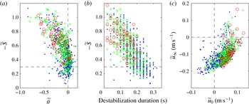
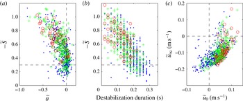
The example just described in detail provides strong indications that the initiation of a rapid plug-type destabilization corresponds to a Sleath number exceeding a threshold value around
 $0.3$
. This needs to be systematically confirmed with other experimental runs. Experiments considered in Berni et al. (Reference Berni, Barthélemy and Michallet2013) are used at this end. For each experiment, moments where the erosion rate exceeds the threshold of 6, 8 or
 $12~\text{mm}~\text{s}^{-1}$
are detected. The Sleath number, the shear stress and the near-bed and free-stream velocities are estimated at these moments and plotted in figure 13 along with the duration of this destabilization defined as the time lapses for which erosion rate exceeds
 $6$
,
 $8$
or
 $12~\text{mm}~\text{s}^{-1}$
. Most of the bed destabilization events are associated with Sleath numbers above the threshold value
 $K_{f}\hspace{2.22198pt}C=0.3$
. Increasing the threshold, for instance to 0.4, would certainly exclude some of the longest events but not modify the qualitative analysis of the relation between pressure gradients and plug-type destabilization. The duration of the destabilization decreases for higher Sleath numbers. Even if the duration seems sensitive to the Sleath threshold, the global trend is not.
As already discussed these plug destabilization events do not correspond to high fluid shear stresses or high velocities. They take place around flow reversal, for negative values of free-stream velocities but, because of the boundary layer phase lead effects, to positive values of near-bed velocity.
Histograms of erosion rates for Sleath number thresholds of
 $0.1$
(a),
 $0.3$
(b) and
 $0.5$
(c). In black, erosion rate value at the time
 $\widetilde{S}$
reaches threshold; in grey, average erosion rate in time lapse during which
 $\widetilde{S}$
exceeds threshold.
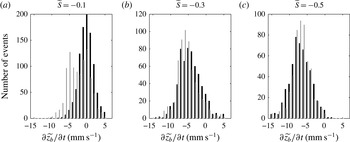
The former analysis showed that destabilization events are associated with Sleath numbers exceeding the plug flow formation criterion. Conversely are Sleath number threshold exceedance events always associated with rapid bed erosion and destabilization? Moments where the Sleath number exceeds the thresholds of
 $0.1$
,
 $0.3$
or
 $0.5$
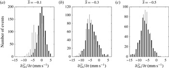
are detected in the data. Histograms of the erosion rate at these specific times and the averaged erosion rate during the exceedance time interval, are presented in figure 14. A threshold of
 $0.1$
as suggested by Foster et al. (Reference Foster, Bowen, Holman and Natoo2006) seems less conclusive. Indeed the distribution associated with
 $-\widetilde{S}$
reaching the
 $0.1$
threshold has a peak for erosion rates close to zero, whereas the most probable erosion rate is approximately 6 mm s
 $^{-1}$
for both
 $-\widetilde{S}=0.3$
and
 $-\widetilde{S}=0.5$
. The statistics associated with the
 $0.3$
and
 $0.5$
thresholds are very similar. Of course there are less ‘
 $-\widetilde{S}\geqslant 0.5$
’ events but the average and standard deviations of the erosion rate are very close in both cases.
In this section we evidenced that strong asymmetric flow velocities, associated with strong pressure gradients in the bed of particles, trigger plug flow and that bed erosion rates are adequate proxies for plug flow formation in non-cohesive sediments. Moreover a striking result is that even though the Shields number reaches negative values as high as those of the Sleath number, the associated resisting shearing effect during rapid plug flow events is negligible. Surprisingly these large Shields number negative values occur at moments when the near-bed velocity
 $\tilde{u} _{0}$
is positive.
6 Vertical pressure gradient effects on bed dynamics
We just showed that the horizontal pressure gradient is the driving force for bed destabilization so that sediment starts moving as a plug at the wave fronts. Without claiming to fully describe the two-phase flow dynamics after plug motion inception, equation (2.2) nevertheless provides further insight into the relative magnitude of competing effects. Amongst these effects the vertical pressure gradients, while neglected for plug motion initiation, will compete with the fluid shear stress as exemplified by equations (2.2) and (2.3). Indeed it is common knowledge (e.g. Nielsen Reference Nielsen1992) in boundary layer flows that
 $\unicode[STIX]{x1D70C}\unicode[STIX]{x2202}u/\unicode[STIX]{x2202}t$
is close, in order of magnitude, to
 $-\unicode[STIX]{x2202}p/\unicode[STIX]{x2202}x$
thus leaving the other three terms in (2.2) to balance.
Time series of (a) the free-surface elevation
 $\widetilde{\unicode[STIX]{x1D702}}$
, (b) the pressure
 $\widetilde{p}$
measured at elevations close to the bed (solid line) and 1.2 cm below (dashed) and (c) the resulting vertical force
 $\widetilde{R_{N}}$
(bold line), composed of the effective weight (
 $Cg\unicode[STIX]{x0394}\unicode[STIX]{x1D70C}\widetilde{\unicode[STIX]{x1D6FF}_{s}}$
, dashed line) and the vertical pressure difference in excess to the hydrostatic pressure between these two elevations (
 $\unicode[STIX]{x0394}\widetilde{p^{\ast }}$
, thin line). The grey strips correspond to times of rapid bed erosion (as in figures 11 and 12).
 $\widetilde{R_{N}}>0$
corresponds to a downward oriented force.
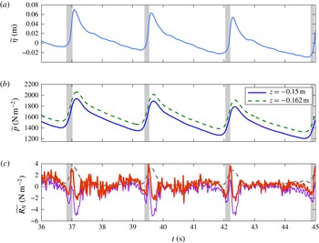
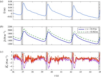
Three wave periods are shown in figure 15 along with the pressure difference measured by sensors located close to the bed interface and 1.2 cm below. The excess pore pressure
 $\unicode[STIX]{x0394}\widetilde{p^{\ast }}$
between the two sensors is compared to the effective weight of the particles of the mobile layer
 $Cg\unicode[STIX]{x0394}\unicode[STIX]{x1D70C}\widetilde{\unicode[STIX]{x1D6FF}_{s}}$
in figure 15(c). The signal is admittedly noisy but the pressure time variations nevertheless show repeatability from wave to wave and run to run.
The measured excess vertical pressure difference is seen to be not large enough to liquefy the whole bed layer between the two sensors (the corresponding effective weight of bed is
 $10.8~\text{N}~\text{m}^{-2}$
) but it is of the same order as the weight of the mobile layer. A delay in pressure transmission (see e.g. Liu et al.
Reference Liu, Park and Lara2007) within the bed at the end of the wave trough contributes to the decrease of the vertical force
 $\widetilde{R_{N}}$
acting on the bed. This likely facilitates the motion inception by reducing the friction at the bottom of the plug. Notice that
 $\widetilde{R_{N}}\simeq 0$
at plug inception in figure 15(c).
Just before the wave crests (close to plug flow end), as the pressure is still increasing in the water column, and horizontal pressure gradients abruptly decrease with flow acceleration, the vertical pressure difference is peaking to approximately zero. This stage of maximum downwards resulting force corresponds to the cessation of bed erosion increase (figure 12).
Just after wave crests, as the pressure in the water column decreases, the delay in pressure transmission within the bed produces a reduction in the resulting vertical force. The settling mobile layer is probably partially liquefied at this stage since
 $\widetilde{R_{N}}<0$
.
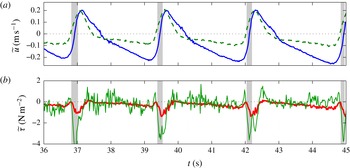
While it was shown in § 5 that plug existence is mainly a question of horizontal pressure gradient exceeding the resultant of the vertical forces, closing the balance in (2.2) involves sums and differences of terms that are close in value during plug flow. However, we qualitatively show in the present section that valuable information can be retrieved from combined analysis of the measurements and equation (2.2). This is summarized in figure 16.
The shear stress
 $\widetilde{\unicode[STIX]{x1D70F}}$
is on one hand directly estimated from the velocity measurements using (4.4) and, on the other hand, obtained with (2.2) in which the other terms are computed from horizontal velocity, layer thickness and pressure measurements. The estimations with (2.2) give overall stronger fluctuations than those with (4.4). Noteworthy are the negative values during plug motion for both estimates, even though (2.2) tends to overestimate the negative peak value of
 $\widetilde{\unicode[STIX]{x1D70F}}$
. After plug motion, when the mobile layer stops thickening and when the bottom velocity reaches its peak, the shear stress reaches its maximum negative value. The top shear stress stays negative until the near-bottom velocity goes to zero. During the entire duration of positive near-bottom velocity,
 $\widetilde{\unicode[STIX]{x1D70F}}$
is negative indicating that the flow above the mobile layer is resisting the forward motion of the mobile layer.
7 Conclusions
The present experiments combined acoustic, optic and piezoelectric sensors in order to simultaneously detect particle motion, measure flow velocities and pressure inside a sediment-bed mobile layer. We show in detail how to process the acoustic intensities of the ADVP to detect both the top of the mobile layer and the still bed interface. The acoustic interface detection was cross-validated with the optical fibre measurements. Extensive repetitions of the same experiments on an overall equilibrium bed profile enable phase-averaging processing to yield accurate results. The bed evolutions are thus been tracked and discussed in terms of balance between momentum and forces acting on a block of bed sediment. The choice of using a lightweight sediment has been made to fulfil the Shields scaling in order to reproduce sheet flow regimes. Another consequence is that the density of the mobile bed varies in a narrow range (
 $1<\unicode[STIX]{x1D70C}_{m}\leqslant 1.09~\text{kg}~\text{l}^{-1}$
), substantiating the use of the model presented in § 2.
The turbulent fluctuations characteristics are in good agreement with those presented in former studies (van der A et al. (Reference van der A, O’Donoghue, Davies and Ribberink2011, for example)). Noteworthy is the weak contribution of the Reynolds stress to the bed shear stress. In addition, the bed shear stress is shown at wave crest phases to be negative indicating that the fluid counteracts on the bed motion. This probably has strong and unexpected practical implications in the use of sediment transport formulas based on the Shields number.
The bed destabilization under wave fronts are shown to be triggered by the horizontal pressure gradient associated with the large flow acceleration of asymmetric waves. Bed destabilization events comply with the criterion proposed by Sleath (Reference Sleath1999) and are ahead of phases during which the velocity shear exceeds the Shields criterion of incipient motion. Strong erosion rates are the consequence of high horizontal pressure gradients whereas slower erosion rates during wave troughs are driven by the fluid shear stress at the top of the mobile layer. During the latter, the dimensionless mobile layer thicknesses measured in the experiments are proportional to the Shields number.
Vertical pressure gradients inside the bed of sediment, mostly due to wave associated water depth variations, are also important for the mobile bed layer dynamics in our experiments. Negative pressure gradients are measured to favour plug flow by decreasing the friction at the base of the slipping block. How strongly this uplift force modifies sediment transport still needs to be investigated.
Acknowledgements
This work was partly funded by the Hydro-Fond project, with the support of the Department of Ecology, sustainable development, transports and housing, general direction of substructures, transports and the sea, within the C2D2 program of RGCU, with additional support of INSU-LEFE. The technical support of J.-M. Barnoud and M. Lagauzère is gratefully acknowledged. The authors are also grateful to the reviewers for their comments that led to significant improvements of the paper.
Appendix A. Bed detection with acoustics
The analysis of the back-scattered acoustic wave train intensity aims at detecting the location of the mobile bed layer. It relies on the observation that a dense mobile layer strongly reflects acoustic waves. Besides, the time variation of the reflection intensity indicates if the particles of the bed are moving or not. As for velocities, each measure is the result of an average over 32 pulses. The analysis involves three different time scales. The first one, noted
 $t_{e}$
, is the time scale that corresponds to the carrier wave frequency (
 $t_{e}<1/2f_{0}$
). The second one (
 $t_{r}$
) corresponds to the time between pulses (
 $1/1600~\text{s}$
). The last one (
 $t=32\;t_{r}$
) corresponds to the actual time resolution of 50 Hz. We analyse the signal for each gate – i.e. each sampling volume within the vertical – and each of the 32 pulses. The signal measured by one receiver (
 $s$
) is multiplied both by the emitted signal (
 $e$
) and the emitted signal shifted by
 $\unicode[STIX]{x03C0}/2$
:
 $$\begin{eqnarray}\displaystyle & \displaystyle e(t_{e})=A_{e}\cos (\unicode[STIX]{x1D714}_{0}t_{e}), & \displaystyle\end{eqnarray}$$
 $$\begin{eqnarray}\displaystyle & \displaystyle s(t_{e})=A_{s}(t_{e})\cos (\unicode[STIX]{x1D714}_{0}t_{e}+\unicode[STIX]{x1D719}_{D}(t_{e})+\unicode[STIX]{x1D719}^{\prime }(t_{e})). & \displaystyle\end{eqnarray}$$
The two resulting signals
 $s_{q}$
and
 $s_{i}$
can be written (Bricault Reference Bricault2006):
 $$\begin{eqnarray}\displaystyle s_{i}(t_{e}) & = & \displaystyle KA_{s}(t_{e})A_{e}\cos (\unicode[STIX]{x1D714}_{0}t_{e})\cos (\unicode[STIX]{x1D714}_{0}t_{e}+\unicode[STIX]{x1D719}_{D}(t_{e})+\unicode[STIX]{x1D719}^{\prime }(t_{e}))\end{eqnarray}$$
 $$\begin{eqnarray}\displaystyle & = & \displaystyle {\textstyle \frac{1}{2}}KA_{s}(t_{e})A_{e}[\cos (2\unicode[STIX]{x1D714}_{0}t_{e}+\unicode[STIX]{x1D719}_{D}(t_{e})+\unicode[STIX]{x1D719}^{\prime }(t_{e}))+\cos (\unicode[STIX]{x1D719}_{D}(t_{e})+\unicode[STIX]{x1D719}^{\prime }(t_{e}))],\end{eqnarray}$$
 $$\begin{eqnarray}\displaystyle s_{q}(t_{e}) & = & \displaystyle KA_{s}(t_{e})A_{e}\cos \left(\unicode[STIX]{x1D714}_{0}t_{e}+\frac{\unicode[STIX]{x03C0}}{2}\right)\cos (\unicode[STIX]{x1D714}_{0}t+\unicode[STIX]{x1D719}_{D}(t_{e})+\unicode[STIX]{x1D719}^{\prime }(t_{e}))\end{eqnarray}$$
 $$\begin{eqnarray}\displaystyle & = & \displaystyle {\textstyle \frac{1}{2}}KA_{s}(t_{e})A_{e}\;[-\sin (2\unicode[STIX]{x1D714}_{0}t_{e}+\unicode[STIX]{x1D719}_{D}(t_{e})+\unicode[STIX]{x1D719}^{\prime }(t_{e}))+\sin (\unicode[STIX]{x1D719}_{D}(t_{e})+\unicode[STIX]{x1D719}^{\prime }(t_{e}))],\end{eqnarray}$$
where
 $\unicode[STIX]{x1D714}_{0}=2\unicode[STIX]{x03C0}f_{0}$
,
 $A_{e}$
the emitted signal amplitude,
 $A_{s}(t_{e})$
the amplitude of the received signal,
 $\unicode[STIX]{x1D719}^{\prime }$
the phase induced by the reflection and
 $K$
a multiplicative gain.
 $\unicode[STIX]{x1D719}_{D}$
is the Doppler phase that verifies
 $\unicode[STIX]{x2202}\unicode[STIX]{x1D719}_{D}/\unicode[STIX]{x2202}t=2\unicode[STIX]{x03C0}f_{D}$
with
 $f_{D}$
the Doppler frequency shift. Maximum velocities
 $U_{max}$
in the flume are of the order of
 $1~\text{m}~\text{s}^{-1}$
. The sound velocity in water is
 $c_{s}=1460~\text{m}~\text{s}^{-1}$
, thus, the maximum Doppler frequency shift is
 $U_{max}f_{0}/c_{s}=f_{0}/1460$
. The gate duration is
 $4/f_{0}$
, and over this duration, the Doppler phase can be considered as constant. The two signals
 $s_{i}$
and
 $s_{q}$
are then low pass filtered, which yields the following for the two signals
 $i(z,t_{r})$
and
 $q(z,t_{r})$
, sampled at
 $f_{r}$
frequency:
 $$\begin{eqnarray}\displaystyle i(z,t_{r}) & = & \displaystyle {\textstyle \frac{1}{2}}KA_{s}(z,t_{r})A_{e}\cos (\unicode[STIX]{x1D719}_{D}(z,t_{r})+\unicode[STIX]{x1D719}^{\prime }(z,t_{r}))\end{eqnarray}$$
 $$\begin{eqnarray}\displaystyle & = & \displaystyle A(z,t_{r})\cos (\unicode[STIX]{x1D719}_{D}(z,t_{r})+\unicode[STIX]{x1D719}^{\prime }(z,t_{r})),\end{eqnarray}$$
 $$\begin{eqnarray}\displaystyle q(z,t_{r}) & = & \displaystyle {\textstyle \frac{1}{2}}KA_{s}(z,t_{r})A_{e}\sin (\unicode[STIX]{x1D719}_{D}(z,t_{r})+\unicode[STIX]{x1D719}^{\prime }(z,t_{r}))\end{eqnarray}$$
 $$\begin{eqnarray}\displaystyle & = & \displaystyle A(z,t_{r})\sin (\unicode[STIX]{x1D719}_{D}(z,t_{r})+\unicode[STIX]{x1D719}^{\prime }(z,t_{r})).\end{eqnarray}$$
These signals are computed at each time step
 $t$
at 50 Hz, for each altitude
 $z$
and each of the 32 pulses
 $n$
(corresponding to different
 $t_{r}$
):
 $$\begin{eqnarray}\displaystyle & \displaystyle i(z,t,n)=A(z,t)\cos (\unicode[STIX]{x1D719}_{D}(z,t)+\unicode[STIX]{x1D719}^{\prime }(z,t,n)), & \displaystyle\end{eqnarray}$$
 $$\begin{eqnarray}\displaystyle & \displaystyle q(z,t,n)=A(z,t)\sin (\unicode[STIX]{x1D719}_{D}(z,t)+\unicode[STIX]{x1D719}^{\prime }(z,t,n)). & \displaystyle\end{eqnarray}$$
The velocity is assumed to be constant over the 32 pulses (i.e. for 20 ms) so that the Doppler phase
 $\unicode[STIX]{x1D719}_{D}$
does not depend on
 $n$
. The amplitude of the received signal
 $A_{s}$
is also assumed to be constant over the
 $n$
pulses. It means that we assume that concentration profile of sediment and bubbles does not evolve significantly over 20 ms.
The back-scattered signal energy profile
 $I_{t}(z,t)$
(or total intensity) is defined as:
 $$\begin{eqnarray}I_{t}(z,t)=\frac{1}{32}\hspace{2.22198pt}\mathop{\sum }_{n=1}^{32}(i(z,t,n)^{2}+q(z,t,n)^{2})\end{eqnarray}$$
and the back-scattered signal energy variance profile
 $I_{v}(z,t)$
(or variance intensity) as:
 $$\begin{eqnarray}I_{v}(z,t)=\frac{1}{32}\hspace{2.22198pt}\mathop{\sum }_{n=1}^{32}\left[\left(i(z,t,n)-\overline{i(z,t)}\right)^{2}+(q(z,t,n)-\overline{q(z,t)})^{2}\right],\end{eqnarray}$$
where
 $\overline{i(z,t)}$
is the average of
 $i(z,t,n)$
over the
 $32$
pulses.
We first consider the most simple case. The ADVP is placed vertically over a sediment bed without any flow nor tracers in the fluid. At each pulse, the received signal amplitude is zero except at the elevation of the bed
 $z_{b}$
(corresponding to the time needed for the acoustic wave to go from the emitting ceramic down to the bed then back to the receivers) and is constant with time. For each pulse, the configuration is the same and the signal obtained is:
 $$\begin{eqnarray}\displaystyle & \displaystyle i(z,t,n)=q(z,t,n)=0,\quad \text{if }z\neq z_{b}, & \displaystyle\end{eqnarray}$$
 $$\begin{eqnarray}\displaystyle & \displaystyle i(z_{b},t,n)=A(z_{b})\cos (\unicode[STIX]{x1D719}^{\prime }(z_{b},t,n)), & \displaystyle\end{eqnarray}$$
 $$\begin{eqnarray}\displaystyle & \displaystyle q(z_{b},t,n)=A(z_{b})\sin (\unicode[STIX]{x1D719}^{\prime }(z_{b},t,n)). & \displaystyle\end{eqnarray}$$
The Doppler phase is equal to zero and the phase induced by the reflection is unchanged throughout time and pulses so that
 $\unicode[STIX]{x1D719}^{\prime }(z_{b},t,n)=\unicode[STIX]{x1D719}^{\prime }(z_{b})$
and:
 $$\begin{eqnarray}\displaystyle I_{t}(z_{b},t) & = & \displaystyle \displaystyle \frac{1}{32}\hspace{2.22198pt}\mathop{\sum }_{n=1}^{32}\left((A(z_{b})\cos (\unicode[STIX]{x1D719}^{\prime }(z_{b})))^{2}+(A(z_{b})\sin (\unicode[STIX]{x1D719}^{\prime }(z_{b})))^{2}\right)\end{eqnarray}$$
 $$\begin{eqnarray}\displaystyle & = & \displaystyle A^{2}(z_{b}),\end{eqnarray}$$
 $$\begin{eqnarray}\displaystyle \overline{i}(z_{b},t) & = & \displaystyle i(z_{b},t,n),\end{eqnarray}$$
 $$\begin{eqnarray}\displaystyle \overline{q}(z_{b},t) & = & \displaystyle q(z_{b},t,n),\end{eqnarray}$$
 $$\begin{eqnarray}\displaystyle I_{v}(z_{b},t) & = & \displaystyle 0.\end{eqnarray}$$
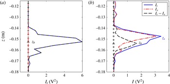
This is illustrated by figure 17(a). The received total intensity is represented as a function of the ceramic distance for a case at rest as specified above. The variance intensity is equal to zero all over the profile. The total intensity is zero until it reaches the bed level. It takes at this specific elevation
 $z_{b}$
a maximum value and then decreases within the bed. The spatial resolution resulting of the gate duration of
 $4~\unicode[STIX]{x03BC}\text{s}$
is 3 mm. It is illustrated by the small vertical black lines on the horizontal axes.
Examples of intensities recorded with the ADVP for a bed at rest (a) and a moving bed (b). The pluses are the locations of the gates at which velocities are measured, the triangles and the star are the estimated locations of the non-moving bed and the top of the mobile layer, respectively.

A similar analysis can be performed for a mobile bed. The velocity is assumed to be constant over one time step. A dense layer of sediment in motion forms (the mobile layer) and the bed elevation
 $z_{b}$
is now defined as the interface between the moving particles and the non-moving ones. In this case, the signals read:
 $$\begin{eqnarray}\displaystyle & \displaystyle i(z,t,n)=A(z,t)\cos (\unicode[STIX]{x1D719}_{D}(z,t)+\unicode[STIX]{x1D719}^{\prime }(z,t,n)), & \displaystyle\end{eqnarray}$$
 $$\begin{eqnarray}\displaystyle & \displaystyle q(z,t,n)=A(z,t)\sin (\unicode[STIX]{x1D719}_{D}(z,t)+\unicode[STIX]{x1D719}^{\prime }(z,t,n)). & \displaystyle\end{eqnarray}$$
Above the bed, if
 $z<z_{b}$
, the Doppler phase is not zero but does not change for one pulse to another, contrary to the phase induced by the reflection as the tracers move. Below the bed, if
 $z>z_{b}$
, as for the case at rest, the Doppler phase is equal to zero and the phase induced by the reflection does not vary. If one assumes that 32 pulses are sufficient for the average of the phase induced by the reflection to converge to zero, the mean of
 $i$
can be expressed as:
 $$\begin{eqnarray}\displaystyle \overline{i}(z<z_{b},t) & = & \displaystyle \frac{1}{32}\hspace{2.22198pt}\mathop{\sum }_{n=1}^{32}\left[A(z,t)\cos \left(\unicode[STIX]{x1D719}_{D}(z,t)+\unicode[STIX]{x1D719}^{\prime }(z,t,n)\right)\right]\end{eqnarray}$$
 $$\begin{eqnarray}\displaystyle & = & \displaystyle 0,\end{eqnarray}$$
 $$\begin{eqnarray}\displaystyle \overline{i}(z>z_{b},t) & = & \displaystyle \frac{1}{32}\hspace{2.22198pt}\mathop{\sum }_{n=1}^{32}\left[A(z,t)\cos \left(\unicode[STIX]{x1D719}^{\prime }(z,t)\right)\right]\end{eqnarray}$$
 $$\begin{eqnarray}\displaystyle & = & \displaystyle A(z,t)\cos (\unicode[STIX]{x1D719}^{\prime }(z,t)),\end{eqnarray}$$
similarly,
 $$\begin{eqnarray}\displaystyle & \displaystyle \overline{q}(z<z_{b},t)=0, & \displaystyle\end{eqnarray}$$
 $$\begin{eqnarray}\displaystyle & \displaystyle \overline{q}(z>z_{b},t)=A(z,t)\sin (\unicode[STIX]{x1D719}^{\prime }(z,t)). & \displaystyle\end{eqnarray}$$
The total and variance intensities therefore read:
 $$\begin{eqnarray}\displaystyle I_{t}(z,t) & = & \displaystyle \frac{1}{32}\hspace{2.22198pt}\mathop{\sum }_{n=1}^{32}\left[A^{2}(z,t)\;\left(\cos ^{2}(\unicode[STIX]{x1D719}_{D}+\unicode[STIX]{x1D719}^{\prime })+\sin ^{2}(\unicode[STIX]{x1D719}_{D}+\unicode[STIX]{x1D719}^{\prime })\right)\right]\end{eqnarray}$$
 $$\begin{eqnarray}\displaystyle & = & \displaystyle A^{2}(z,t),\end{eqnarray}$$
 $$\begin{eqnarray}\displaystyle I_{v}(z<z_{b},t) & = & \displaystyle I_{t}(z,t)\end{eqnarray}$$
 $$\begin{eqnarray}\displaystyle & = & \displaystyle A^{2}(z,t),\end{eqnarray}$$
 $$\begin{eqnarray}\displaystyle I_{v}(z>z_{b},t) & = & \displaystyle 0.\end{eqnarray}$$
An illustration of these signals is given in figure 17(b). For
 $z>0.147~\text{m}$
the total and variance intensities are nearly equal and increase when approaching the bed. After reaching a maximum, the variance intensity decreases faster than the total intensity as predicted by the equations just shown. Theoretically, the still bed elevation
 $z_{b}$
is defined as the elevation where the variance intensity is zero but the total intensity is still high. For practical reason, it will be computed as the maximum of the difference between the total and the variance intensities. A second interface
 $z_{s}$
is defined as the maximum of the total intensity. At rest, these two interfaces merge. When a mobile layer develops,
 $z_{s}$
is identified as being the elevation where the gradient of concentration is the strongest and is interpreted as the upper elevation of the mobile layer.