2.1 Numerical simulation domain

Figure 1.

Model and computational domain of the calculation: (a) structure of the simulation domain and (b) channel cross-section.

The structure of the simulation domain is shown in figure 1(a). The electrodes were placed on the top and bottom of the channel. Figure 1(b) shows that the height of the throat at $X=54.5~\text{mm}$ was 3.55 mm, and the distance between the two cathodes at the location of $X=115~\text{mm}$ was 9.87 mm.

2.2 Mathematical model

2.2.1 Governing equations for MHD (magnetohydrodynamics) plasma flows

The time-dependent compressible Navier–Stokes equations coupled with Lorentz force and energy exchange terms are as follows:

Continuity equation:

(2.1) $$\begin{eqnarray}\displaystyle {\displaystyle \frac{\unicode[STIX]{x2202}\unicode[STIX]{x1D70C}}{\unicode[STIX]{x2202}t}}+\unicode[STIX]{x1D735}\boldsymbol{\cdot }(\unicode[STIX]{x1D70C}\boldsymbol{u})=0. & & \displaystyle\end{eqnarray}$$

Momentum equation:

(2.2) $$\begin{eqnarray}\displaystyle \frac{\unicode[STIX]{x2202}\unicode[STIX]{x1D70C}\boldsymbol{u}}{\unicode[STIX]{x2202}t}+\unicode[STIX]{x1D735}\boldsymbol{\cdot }(\unicode[STIX]{x1D70C}\boldsymbol{u}\boldsymbol{u})=\boldsymbol{j}\times \boldsymbol{B}-\unicode[STIX]{x1D735}p+\unicode[STIX]{x1D735}\boldsymbol{\cdot }\unicode[STIX]{x1D749}. & & \displaystyle\end{eqnarray}$$

Energy equation:

(2.3a,b ) $$\begin{eqnarray}\frac{\unicode[STIX]{x2202}E_{s}}{\unicode[STIX]{x2202}t}+\unicode[STIX]{x1D735}\boldsymbol{\cdot }(E_{s}+p)\boldsymbol{u}=\boldsymbol{j}\boldsymbol{\cdot }\boldsymbol{E}-\unicode[STIX]{x1D735}\boldsymbol{\cdot }\boldsymbol{q}+\unicode[STIX]{x1D735}\boldsymbol{\cdot }(\unicode[STIX]{x1D70F}\boldsymbol{u}),\quad E_{s}=\unicode[STIX]{x1D70C}\left(c_{V}T+{\displaystyle \frac{1}{2}}\boldsymbol{u}^{2}\right),\end{eqnarray}$$

where $\unicode[STIX]{x1D70C}$ is the mass density, $\boldsymbol{u}$ is the velocity vector of the flow, $\boldsymbol{j}$ is the current density vector, $\boldsymbol{B}$ is the magnetic flux density vector, $p$ is the static pressure, $\unicode[STIX]{x1D70F}$ is the viscous stress, $E_{s}$ is the total energy, $c_{v}$ is the constant volume specific heat, $T$ is the static temperature, $\boldsymbol{E}$ is the electric field vector and $\boldsymbol{q}$ is the conductive heat flux vector.

2.2.2 Governing equations for ionization

The governing equations for ionization were as follows:

Conservation of ion number density:

(2.4) $$\begin{eqnarray}\displaystyle {\displaystyle \frac{\unicode[STIX]{x2202}n_{i}^{+}}{\unicode[STIX]{x2202}t}}+\unicode[STIX]{x1D735}\boldsymbol{\cdot }n_{i}^{+}\boldsymbol{u}=k_{fi}n_{e}n_{i}-k_{ri}n_{e}^{2}n_{i}^{+},\quad n_{e}=n_{1}^{+}. & & \displaystyle\end{eqnarray}$$

Energy equation for electrons:

(2.5) $$\begin{eqnarray}\displaystyle \left.\begin{array}{@{}c@{}}{\displaystyle \frac{\unicode[STIX]{x2202}U_{e}}{\unicode[STIX]{x2202}t}}+\unicode[STIX]{x1D735}\boldsymbol{\cdot }(U_{e}\boldsymbol{u}_{e})={\displaystyle \frac{|\boldsymbol{j}|^{2}}{\unicode[STIX]{x1D70E}}}-p_{e}\unicode[STIX]{x1D735}\boldsymbol{\cdot }\boldsymbol{u}_{e}-3n_{e}k(T_{e}-T)\mathop{\sum }_{h}^{\text{heavy}}{\displaystyle \frac{m_{e}}{m_{h}}}\overline{\unicode[STIX]{x1D708}}_{eh},\\ p_{e}=n_{e}kT_{e},\quad U_{e}={\displaystyle \frac{3}{2}}n_{e}kT_{e}+n_{i}^{+}\unicode[STIX]{x1D700}_{i}.\end{array}\right\} & & \displaystyle\end{eqnarray}$$

In (2.4), $n_{i}^{+}$ is ion number density of argon, $n_{e}$ is electron number density, $n_{i}$ is atom number density of argon, the three-body recombination rate coefficient $k_{r}$ is determined by the following relations (Tanaka, Murakami & Okuno Reference Tanaka, Murakami and Okuno2014):

(2.6) $$\begin{eqnarray}\displaystyle \left.\begin{array}{@{}c@{}}k_{r}=k_{rh}k_{ro}/(k_{rh}+k_{ro}),\quad k_{rh}=1.09\times 10^{-20}{T_{e}}^{-9/2},\quad \\[6.0pt] k_{ro}=3.33\times 10^{-44}\left({\displaystyle \frac{135\,300}{T_{e}}}+2\right)\exp \left({\displaystyle \frac{47\,800}{T_{e}}}\right),\end{array}\right\} & & \displaystyle\end{eqnarray}$$

and the ionization rate coefficient $k_{f}$ is derived based on the principle of a detailed balance with the Saha equilibrium, $k_{f}n_{i}n_{e}=k_{r}n_{i}n_{e}^{2}$ , $k_{f}=k_{r}\times g_{i}/g_{0}(2\unicode[STIX]{x03C0}m_{e}kT_{e}/h^{2})^{3/2}\exp (-\unicode[STIX]{x1D700}_{i}/kT_{e})$ , where $g_{i}$ is the statistical weight of the ground state of the ion, $g_{0}$ is the statistical weight of the ground state of the neutral argon atom, $\unicode[STIX]{x1D700}_{i}$ is the ionization potential of the argon atom (Tanaka et al. Reference Tanaka, Murakami and Okuno2014) and the subscripts $e$ and $i$ and the superscript + denote the electrons, neutral atoms and ions, respectively. In (2.5), $U_{e}$ is the electron energy, $u_{e}$ is the velocity vector of the electrons, $m_{h}$ is the mass of a heavy particle, $m_{e}$ is the mass of an electron, $p_{e}$ is the electron pressure, $k$ is the Boltzmann constant, $T_{e}$ is the electron temperature and $\unicode[STIX]{x1D700}_{i}$ is the ionization energy. The large eddy simulation-Smagorinsky model was applied as the turbulence model for the flow.

2.2.3 Governing electrical and magnetic equations

The governing electrical and magnetic equations are as follows:

Generalized Ohm’s law:

(2.7) $$\begin{eqnarray}\displaystyle \boldsymbol{j}+\frac{\unicode[STIX]{x1D6FD}}{|\boldsymbol{B}|}\boldsymbol{j}\times \boldsymbol{B}=\unicode[STIX]{x1D70E}(\boldsymbol{E}+\boldsymbol{u}\times \boldsymbol{B}),\quad \unicode[STIX]{x1D70E}=\frac{e^{2}n_{e}}{m_{e}\overline{\unicode[STIX]{x1D708}}_{eh}},\quad \unicode[STIX]{x1D6FD}=\frac{e|\boldsymbol{B}|}{m_{e}\overline{\unicode[STIX]{x1D708}}_{eh}}. & & \displaystyle\end{eqnarray}$$

Maxwell equations:

(2.8) $$\begin{eqnarray}\displaystyle \unicode[STIX]{x1D735}\times \boldsymbol{H}=\boldsymbol{j}+\frac{\unicode[STIX]{x2202}\boldsymbol{D}}{\unicode[STIX]{x2202}t},\quad \unicode[STIX]{x1D735}\boldsymbol{\cdot }\boldsymbol{B}=0\unicode[STIX]{x1D735}\times \boldsymbol{E}=-{\displaystyle \frac{\unicode[STIX]{x2202}\boldsymbol{B}}{\unicode[STIX]{x2202}t}},\quad \unicode[STIX]{x1D735}\boldsymbol{\cdot }\boldsymbol{D}=\unicode[STIX]{x1D70C}_{e}. & & \displaystyle\end{eqnarray}$$

Since the charge was assumed to be neutral and the magnetic Reynolds number was quite small, the Maxwell equations were simplified as follows:

(2.9) $$\begin{eqnarray}\displaystyle \unicode[STIX]{x1D735}\times \boldsymbol{E}=0,\quad \unicode[STIX]{x1D735}\boldsymbol{\cdot }\boldsymbol{j}=0. & & \displaystyle\end{eqnarray}$$

In (2.7), $\overline{\unicode[STIX]{x1D708}}_{eh}=\sum _{h}^{\text{heavy}}n_{h}Q_{eh}C_{e}$ is the average momentum transfer collision frequency for an electron $e$ with a heavy particle, where $Q_{eh}$ is the energy-averaged momentum transfer cross-section, $C_{e}=\sqrt{8kT_{e}/\unicode[STIX]{x03C0}m_{e}}$ is the mean electron velocity for a Maxwellian distribution, $\unicode[STIX]{x1D70E}$ is the electrical conductivity and $\unicode[STIX]{x1D6FD}$ is the Hall parameter. In (2.9), $\boldsymbol{E}=-\unicode[STIX]{x1D735}\unicode[STIX]{x1D6F7}$ is the electric field vector, where $\unicode[STIX]{x1D6F7}$ is the electrical potential. The elliptic equations for the potential derived from (2.7) and (2.8) are as follows:

(2.10) $$\begin{eqnarray}\displaystyle \unicode[STIX]{x1D735}\boldsymbol{\cdot }(\unicode[STIX]{x1D70E}\unicode[STIX]{x1D735}\unicode[STIX]{x1D6F7})=\unicode[STIX]{x1D735}\boldsymbol{\cdot }\left(\unicode[STIX]{x1D70E}\boldsymbol{u}\times \boldsymbol{B}+\frac{\unicode[STIX]{x1D6FD}}{|\boldsymbol{B}|}\boldsymbol{j}\times \boldsymbol{B}\right), & & \displaystyle\end{eqnarray}$$

which was solved using the MHD model in the Fluent software. The set of above equations (2.1)–(2.5) was solved numerically by means of a first-order upwind scheme.

2.3 Boundary conditions and numerical procedures

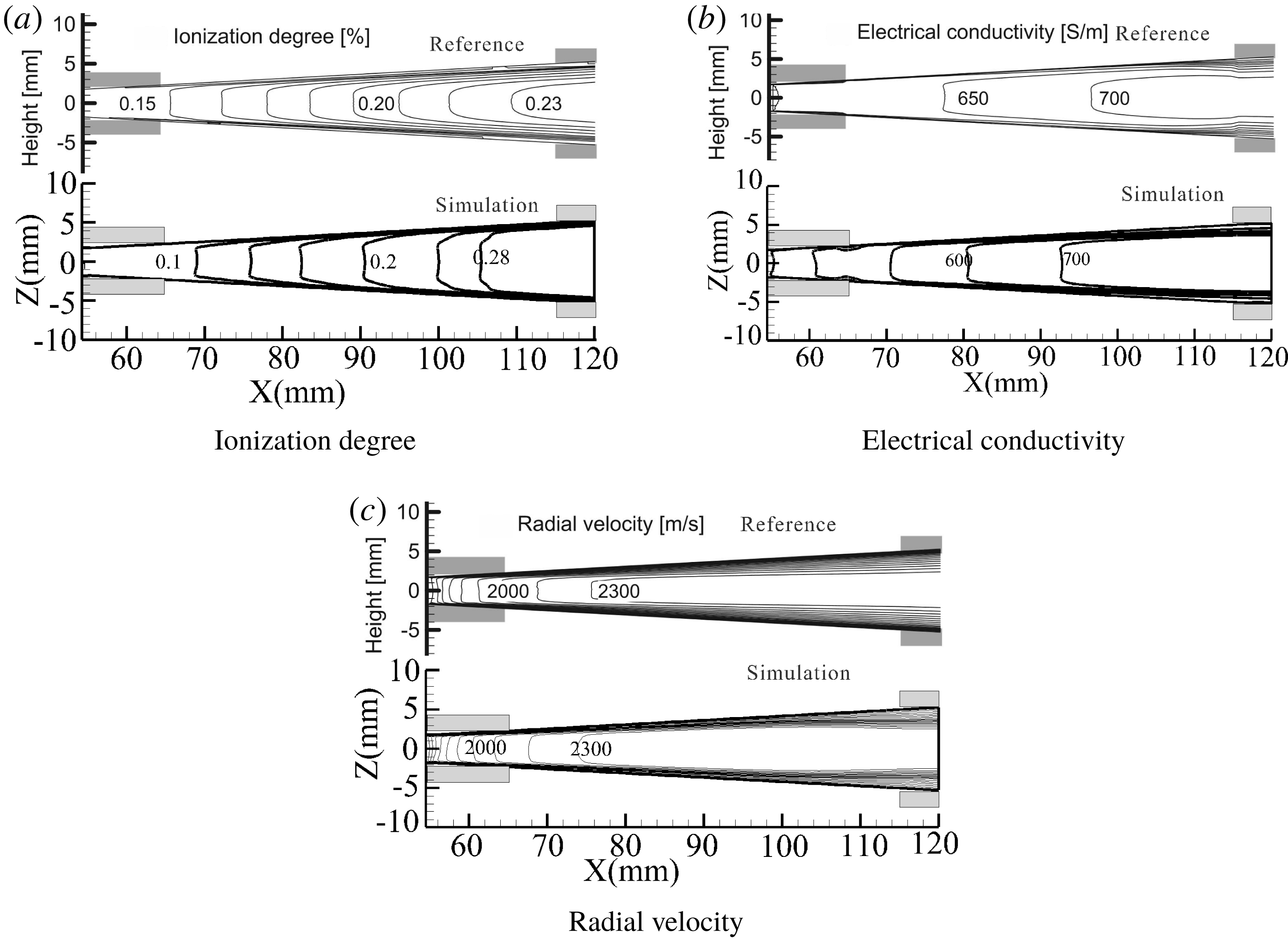
The codes and numerical procedures of simulation are firstly verified by comparing with results from the literature (Harada et al. Reference Harada, Hishikawa, Nara and Sakamoto2005) (figure 2). The comparison shows that, within an acceptable range of error, the code and the program are effective.

Figure 2.

The verification of the simulations.

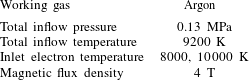
The grid numbers for the channel are $40\times 120\times 100$ in Cartesian coordinates in the $z\times x\times y$ directions. Working gas was assumed to be a pure noble gas in the simulations. The non-equilibrium plasma in the channel consisted of ions, electrons and atoms under a two-temperature model (Mitchner & Kruger Reference Mitchner and Kruger1973; Tanaka et al. Reference Tanaka, Murakami and Okuno2014). The non-equilibrium plasma was described by the combination of state and Maxwell equations. The Navier–Stokes equations were solved using the large eddy simulation method. The no-slip wall of the channel was electrically insulated, and its temperature was set to 300 K. The boundary conditions for the electrical equation were an external voltage on the anode and 0 V on the cathode. Table 1 shows the working conditions of the high-temperature seed-free argon plasma used in the study.

Figure 3.

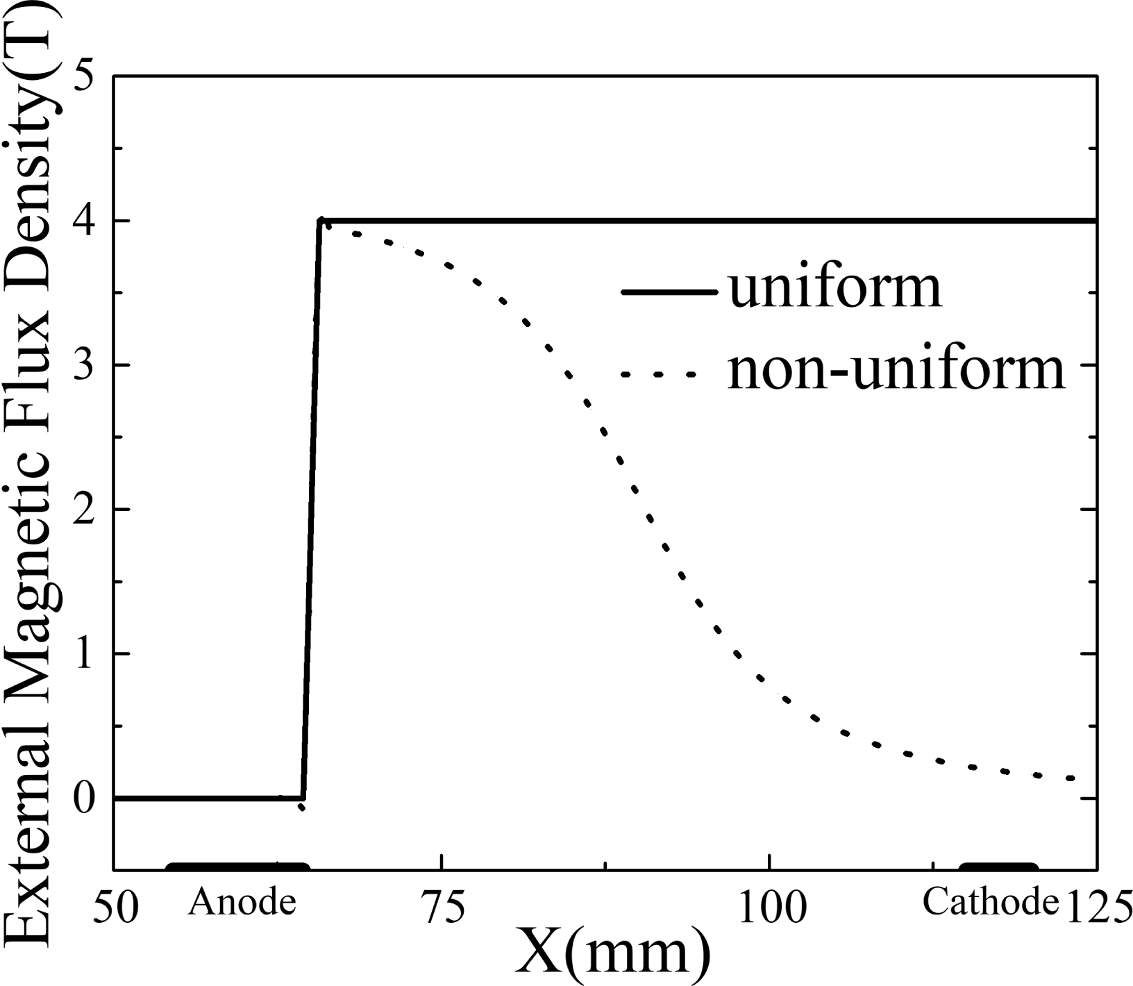
Distribution of external magnetic field.

Table 1.

Conditions used in calculation.

3.1 Different distributions of magnetic field

Due to the influence of the Hall effect, two external magnetic field configurations were considered in the simulations. Figure 3 shows the distribution of the magnetic flux density along the centre line of the channel. The solid line represents the uniform magnetic flux density (4 T). The dashed line is the non-uniform magnetic flux density (0.12–4 T). Both external magnetic fields were confined to the 65–125 mm region.

There were three kinds of currents in the channel,

(3.1) $$\begin{eqnarray}\displaystyle \left.\begin{array}{@{}l@{}}\displaystyle j_{x}=\frac{\unicode[STIX]{x1D70E}}{1+\unicode[STIX]{x1D6FD}^{2}}(E_{x}-\unicode[STIX]{x1D6FD}E_{y}+\unicode[STIX]{x1D6FD}u_{x}B+u_{y}B),\\[13.20007pt] \displaystyle j_{y}=\frac{\unicode[STIX]{x1D70E}}{1+\unicode[STIX]{x1D6FD}^{2}}(\unicode[STIX]{x1D6FD}E_{x}+E_{y}-u_{x}B+\unicode[STIX]{x1D6FD}u_{y}B),\\[13.20007pt] \displaystyle j_{z}=\unicode[STIX]{x1D70E}E_{z},\end{array}\right\} & & \displaystyle\end{eqnarray}$$

where $E_{x}$ and $E_{y}$ are the components of the electric field in the $x$ and $y$ directions, respectively; $j_{x}$ , $j_{y}$ and $j_{z}$ are the components of the current density in the $x,y$ and $z$ directions, respectively; and $u_{x}$ and $u_{y}$ are the components of the flow velocity in the $x$ and $y$ directions, respectively.

Figure 4.

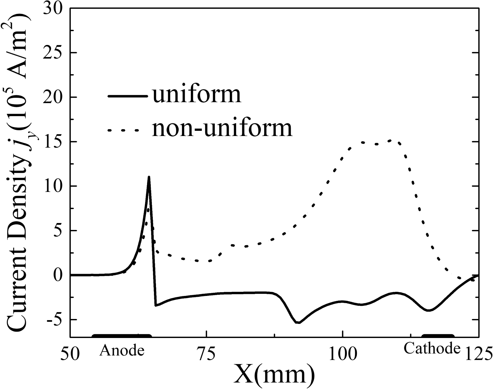
Distribution of tangential current.

Figure 5.

Distribution of Lorentz force.

For a uniform external magnetic field, the value of the main term $u_{x}B_{z}$ increases with the flow velocity. As a result, the current $j_{y}$ decreases to a negative value, resulting in the Lorentz force in the $x$ direction $(F_{x}=j_{y}B_{z})$ decelerating the flow. As shown in figure 4, the current density was less than 0 in the uniform magnetic field. 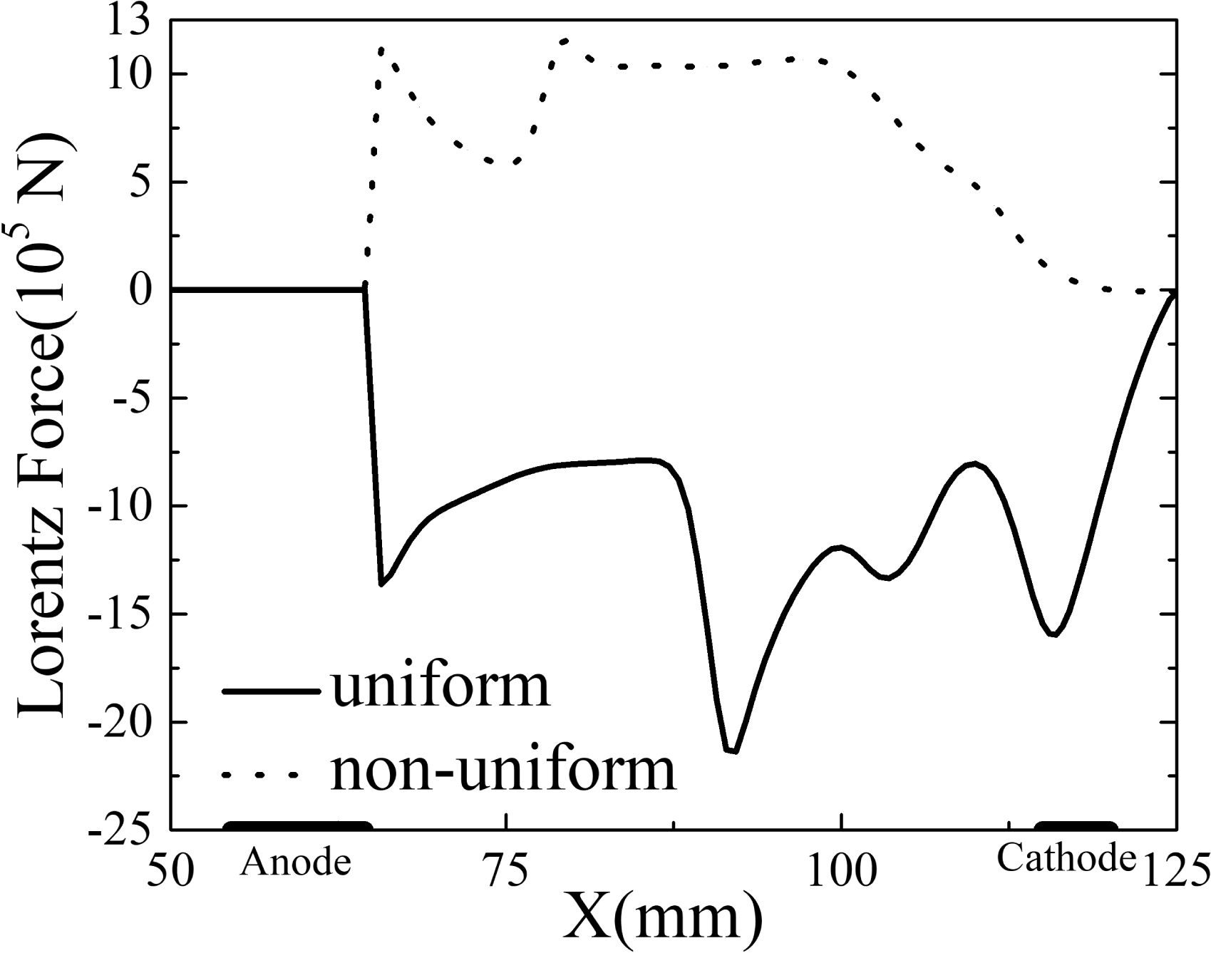On the contrary, the current density $j_{y}$ was always positive in the non-uniform magnetic field until the end of the channel. 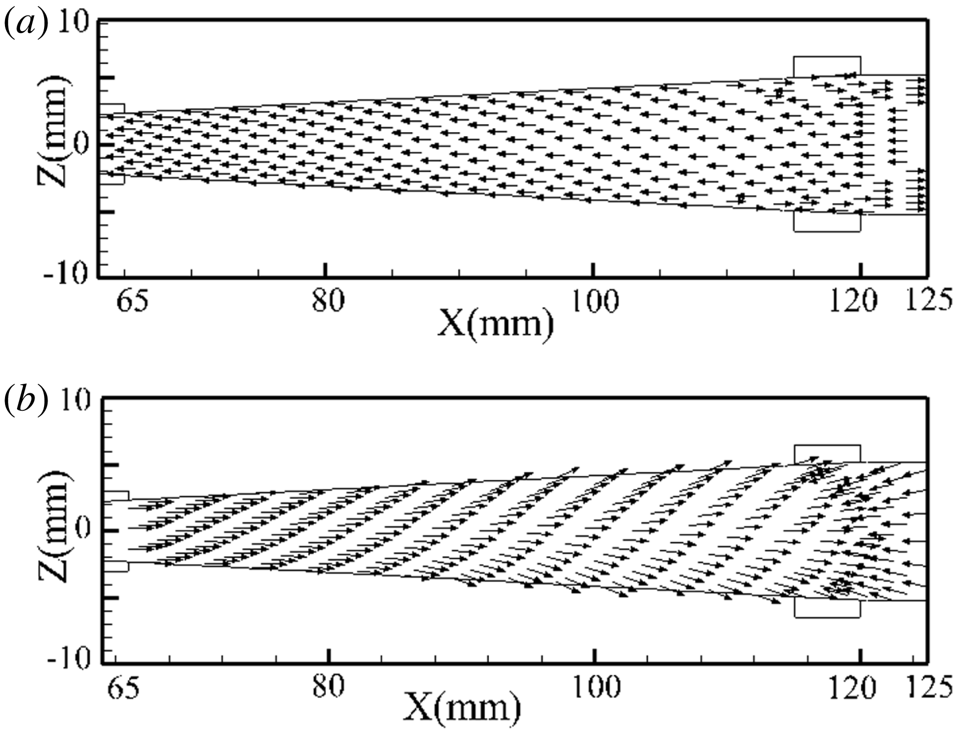With a decaying distribution of the non-uniform magnetic field, figure 5 shows the distribution of the Lorentz force along the centre line of the channel, and the Lorentz force remained in the same direction as the flow because the current density $j_{y}$ was positive, even as the flow velocity increased. Figure 6 provides the vector of the Lorentz force at the XOZ cross-section. From figures 5 and 6, the Lorentz force in the uniform magnetic field was opposite to the flow direction and played a decelerating role. In the non-uniform magnetic field, the Lorentz force was more consistent with the flow direction and played an accelerating role. Thus, the flow was accelerated more by the Lorentz force in the non-uniform magnetic field.

Figure 6.

Vectors of Lorentz force in XOZ cross-section: (a) uniform magnetic field and (b) non-uniform magnetic field.

Figure 7.

Distribution of Hall parameter.

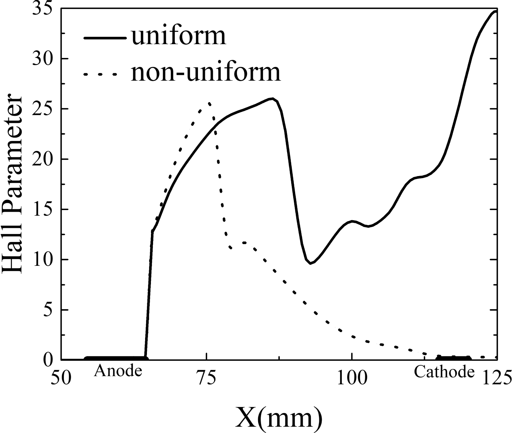
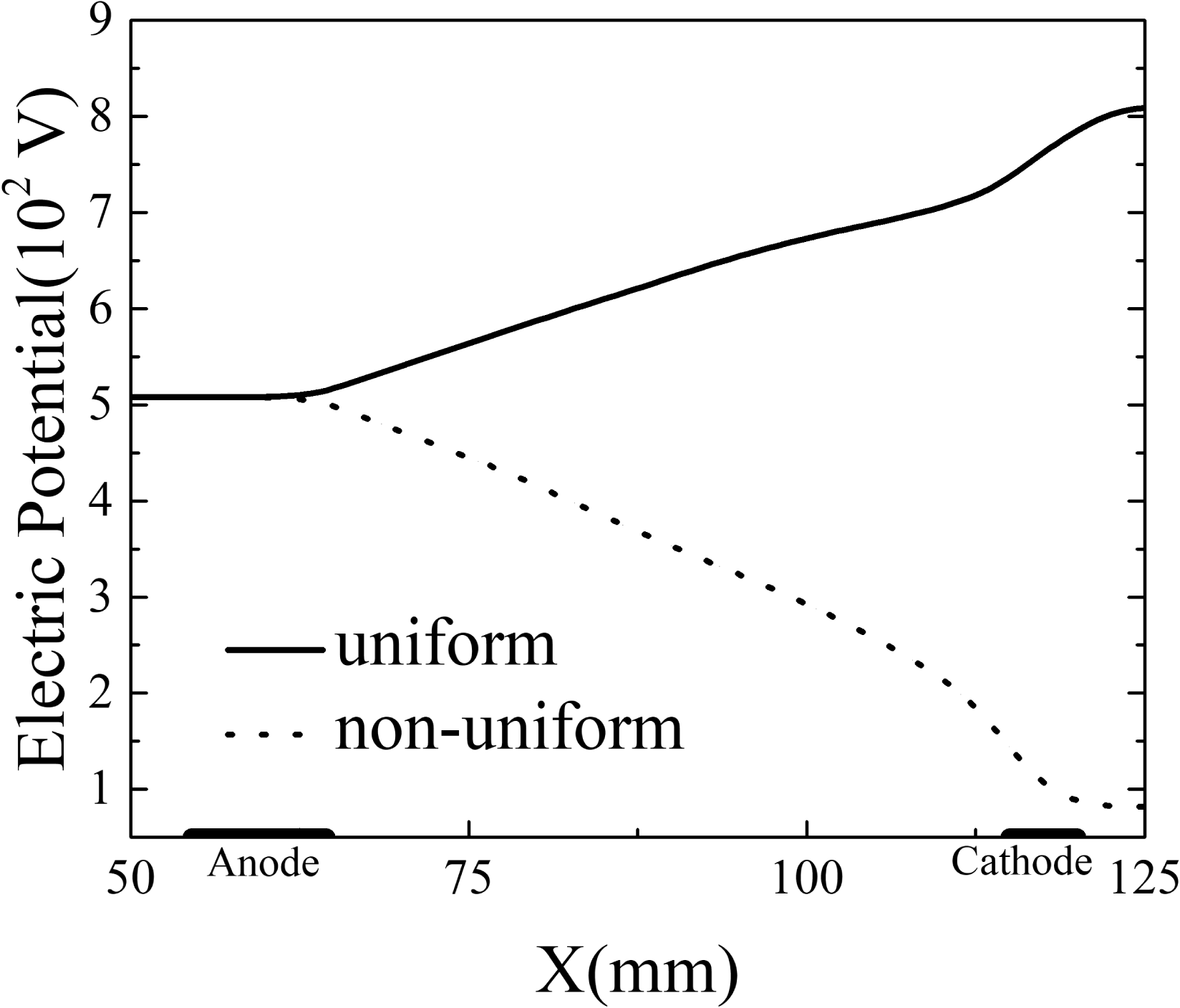
This anomaly can be mainly explained by the stronger Hall effect in the uniform magnetic field. Figure 7 provides the distributions of the Hall parameter in the uniform and non-uniform magnetic fields, which is an important parameter for estimating the magnitude of the Hall effect. The Hall parameter was in the 20–35 range in the uniform magnetic field, but it decreased to nearly 0 at the end of the channel due to the decrease in the magnetic field intensity in the non-uniform magnetic field. Therefore, a larger Hall potential was generated in the uniform magnetic field, which led to electric power generation. Figure 8 shows the distribution of the electrical potential under two magnetic field configurations. Since the intensity of the uniform magnetic field remained unchanged, the Hall potential continued to increase until it exceeded the external potential (the external potential was 508 V, the Hall potential was 808 V), which was deleterious to the acceleration. In the non-uniform magnetic field, the Hall potential was always smaller than the external potential (the external potential was 508 V, the Hall potential was 82 V), which could ensure continued acceleration.

Figure 8.

Distribution of electric potential.

Figure 9.

Distribution of velocity $u_{x}$ .

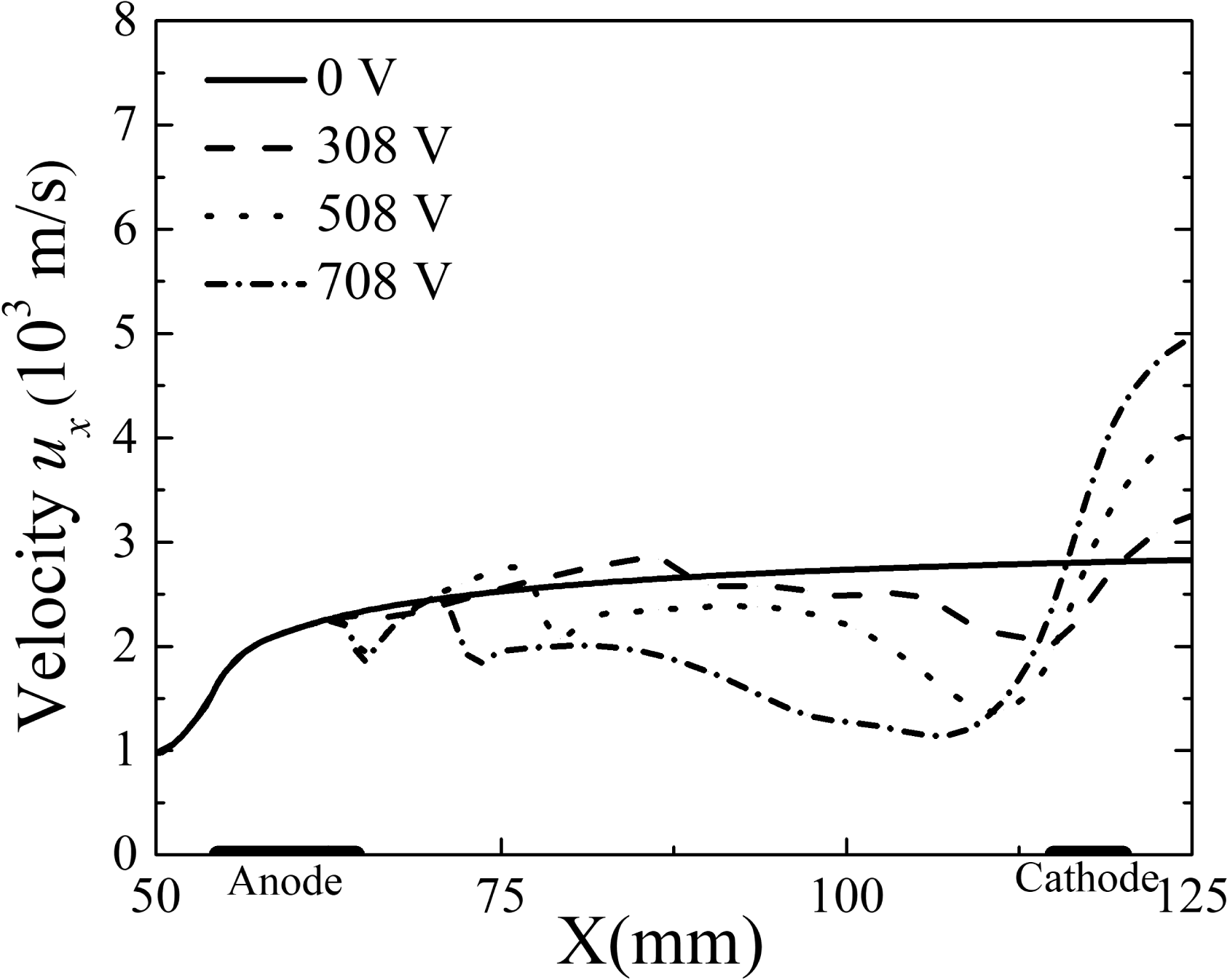
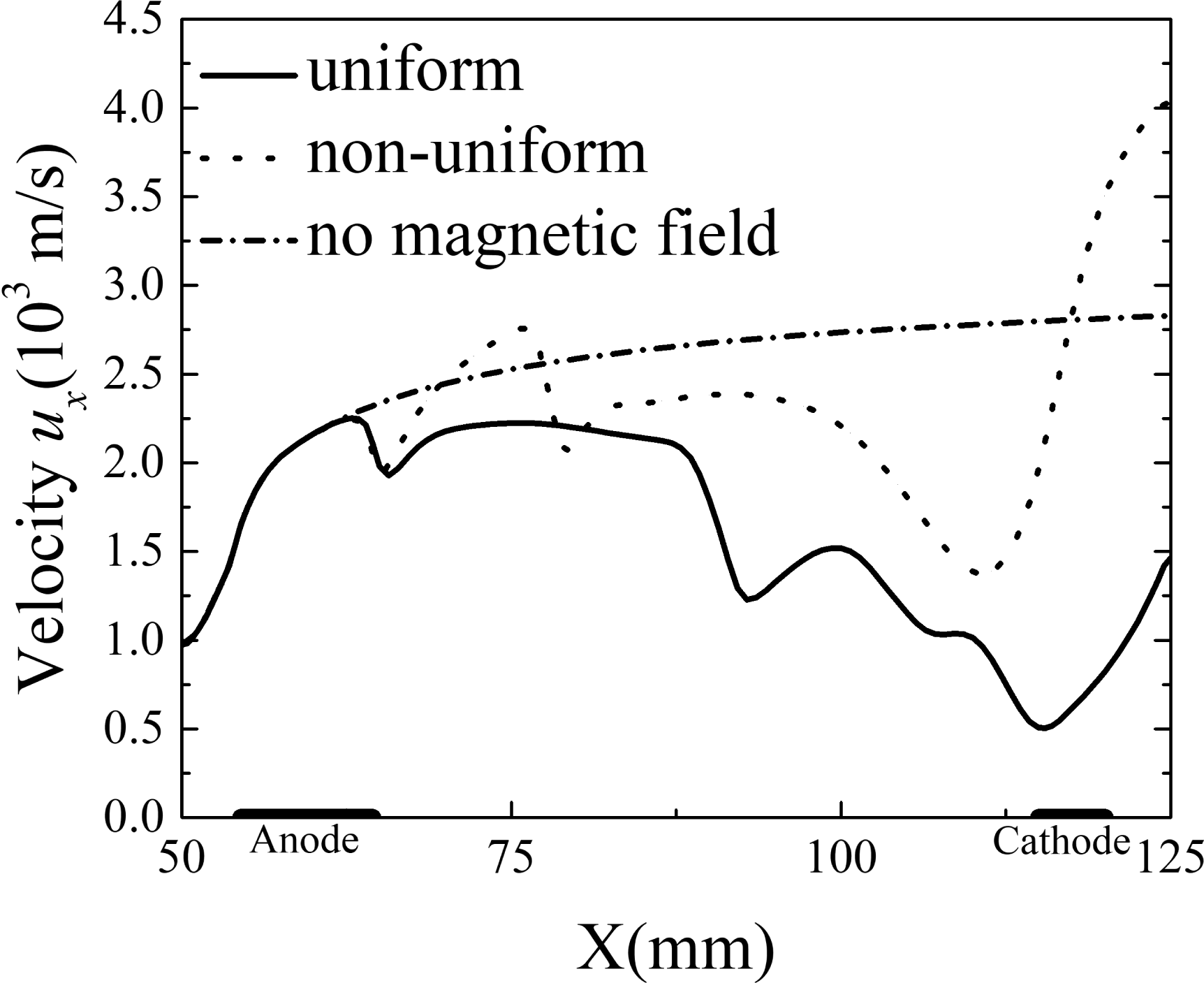
Figure 9 provides the distribution of the velocity $u_{x}$ along the centre line of the channel and shows that the velocity could be increased from $972~\text{m}~\text{s}^{-1}$ at the inlet to $2828~\text{m}~\text{s}^{-1}$ at the exit only by acceleration working of the throat with out electromagnetic interactions. The flow in the uniform magnetic field initially accelerated to approximately $2250~\text{m}~\text{s}^{-1}$ by acceleration working of the throat, the final velocity was only $1463~\text{m}~\text{s}^{-1}$ at the exit because the flow was decelerated by the Lorentz force generated in the uniform magnetic field. 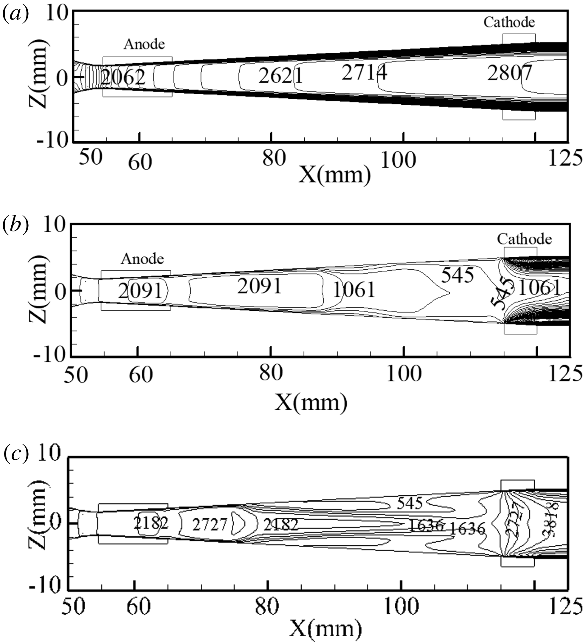The non-uniform magnetic field caused the velocity to increase from $972~\text{m}~\text{s}^{-1}$ at the inlet to $4033~\text{m}~\text{s}^{-1}$ at the exit. Due to the strong electromagnetic coupling, irregularities also appeared in the acceleration process of the non-uniform magnetic field. The acceleration under the non-uniform magnetic field caused boundary separation and reflux at the boundary in the 77–110 mm region, as shown in figure 10(b), which had an adverse effect on the acceleration and resulted in a decrease in the velocity. By comparing the velocities in figure 10, we concluded that the non-uniform magnetic field was more suitable for Hall-effect electromagnetic acceleration. The above results also indicated an effective and significant electromagnetic acceleration performance in the non-uniform magnetic field.

Figure 10.

Contours of velocity $u_{x}$ XOZ cross-section: (a) no magnetic field, (b) uniform magnetic field and (c) non-uniform magnetic field.

3.2 Different applied external electric potentials

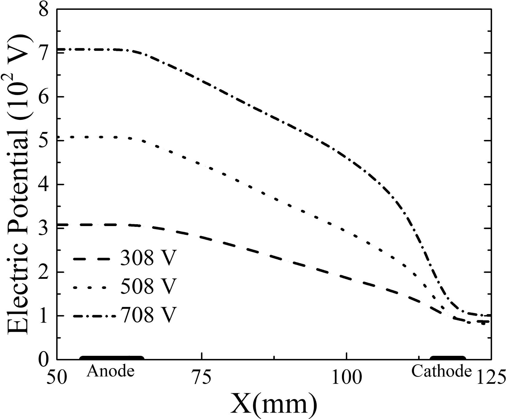
In addition to the influence of the magnetic field, the effect of the different external electric potentials on the acceleration should be considered. Based on the results in the previous section, the simulations discussed in this section were conducted with non-uniform external magnetic fields. As presented in figure 11, three applied external voltages of 308, 508 and 708 V were studied, and the corresponding Hall potential ( $U_{\text{hall}}=\unicode[STIX]{x1D6FD}kvBL$ , where $L$ is the distance between the electrodes and $k$ is the load coefficient) increased as the applied voltage increased. Referring to the definition of the Hall potential, the Hall parameter, load coefficient and velocity were the critical parameters, since $B$ and $L$ were the same in the three cases. As shown in table 2, the average Hall parameter, and the average electric conductivity decreased continually. The Hall potentials were 87, 82, 101 V for the applied external voltages of 308, 508 and 708 V, respectively. It was inferred that the velocity increased as the applied voltage increased.

Figure 11.

Distribution of electrical potential.

Figure 12.

Distribution of Joule heating.

Table 2.

Electric conductivity and Hall parameter.

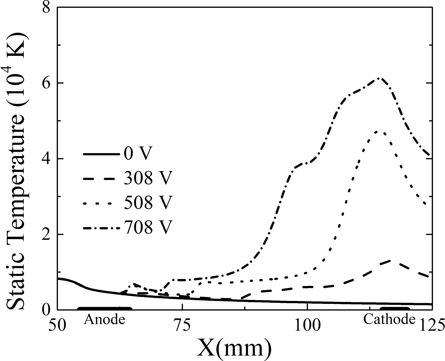
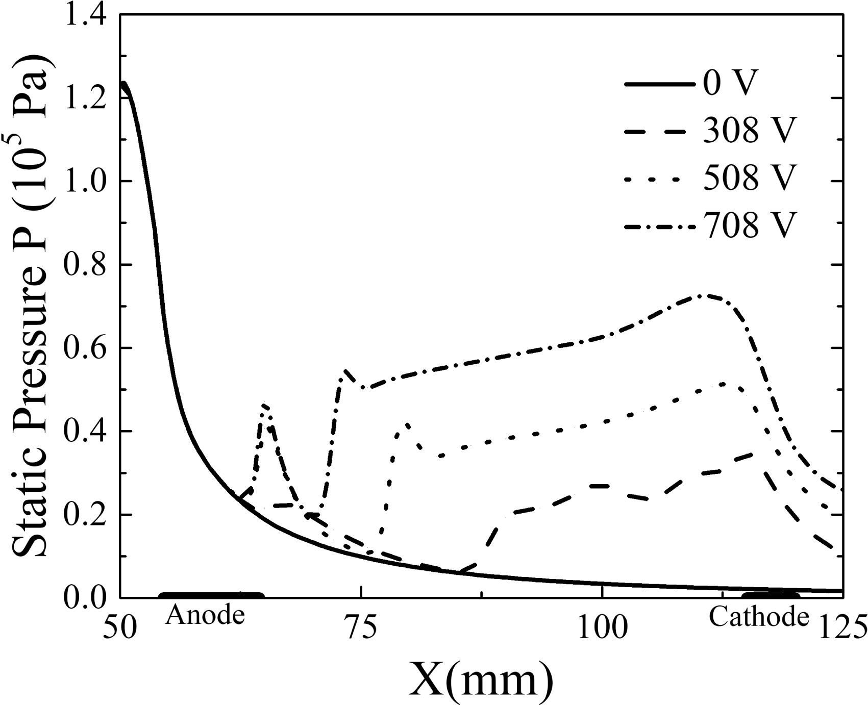
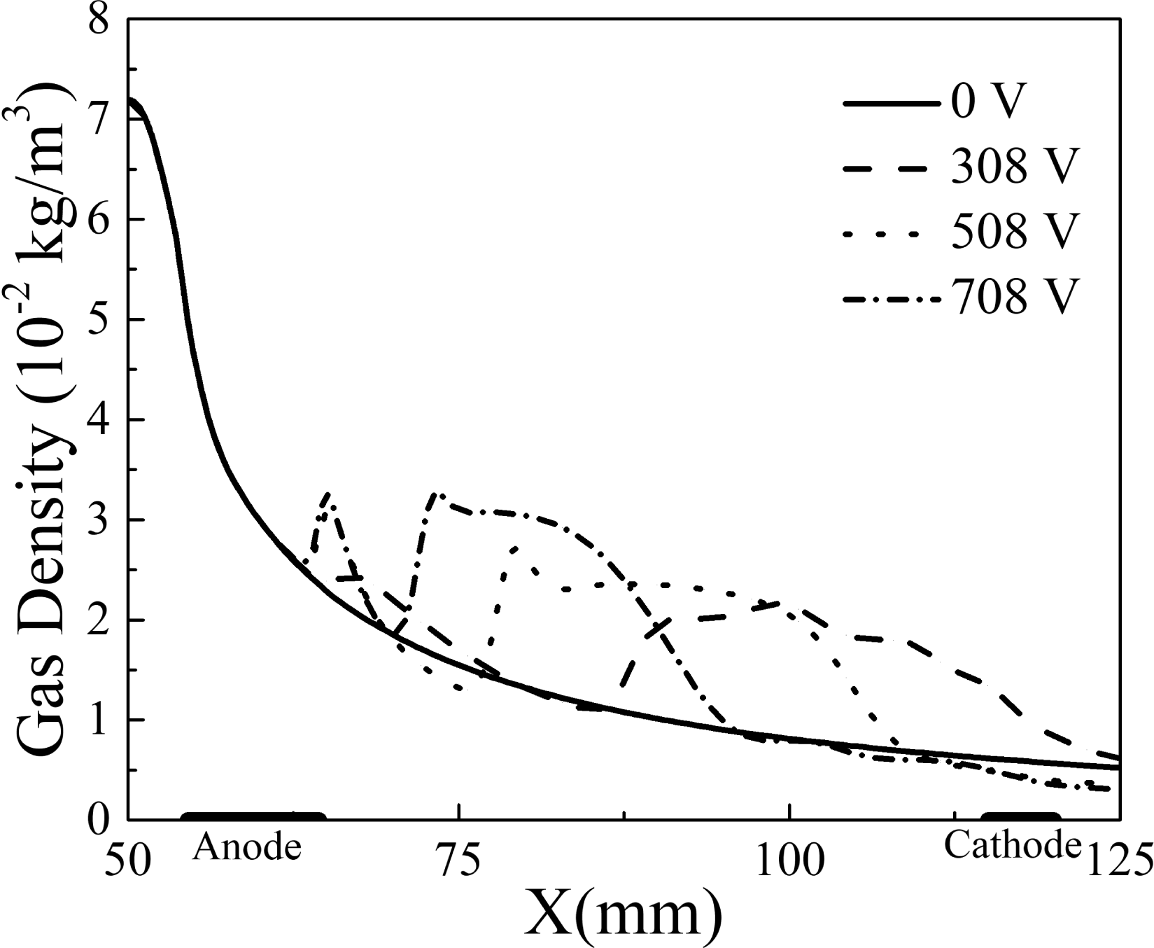
The current density in the channel increased with the external potential, which caused the Joule heating to increase rapidly. The Joule heating increase shown in figure 12 was also affected by the increase in the Hall potential near the cathode. A higher Joule heating magnified the gas internal energy, which resulted in a higher gas temperature (figure 13) and a significantly stronger static pressure, especially near the electrode region (figure 14). As the working gas was assumed to be ideal, unevenness of the gas density in the flow field was generated based on the dramatic changes of the static temperature and static pressure. The gas density was higher than 0 V at positions ranging from 65 to 125 mm at 308 V, 65 to 107 mm at 508 V, 65 to 90 mm at 708 V, respectively, which are shown in figure 15. In contrast, the gas density was smaller than 0 V at positions ranging from 107 to 125 mm at 508 V and 90 to 125 mm at 708 V due to the significant static temperature increment in those positions.

Figure 13.

Distribution of static temperature.

Figure 14.

Distribution of static pressure.

Figure 15.

Distribution of gas density.

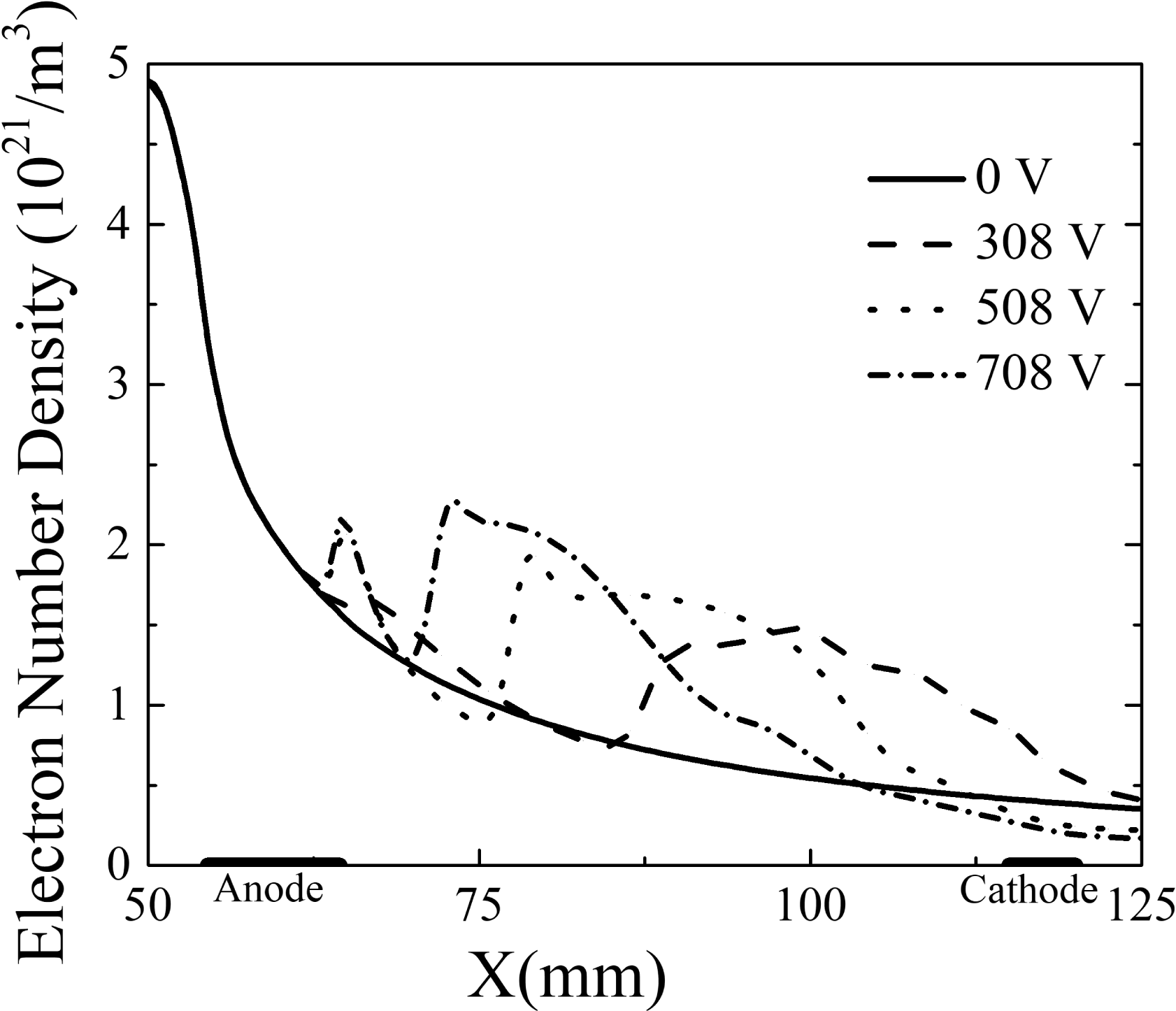
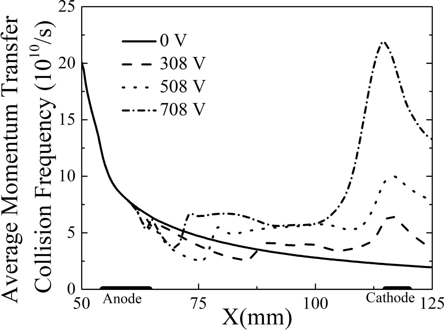
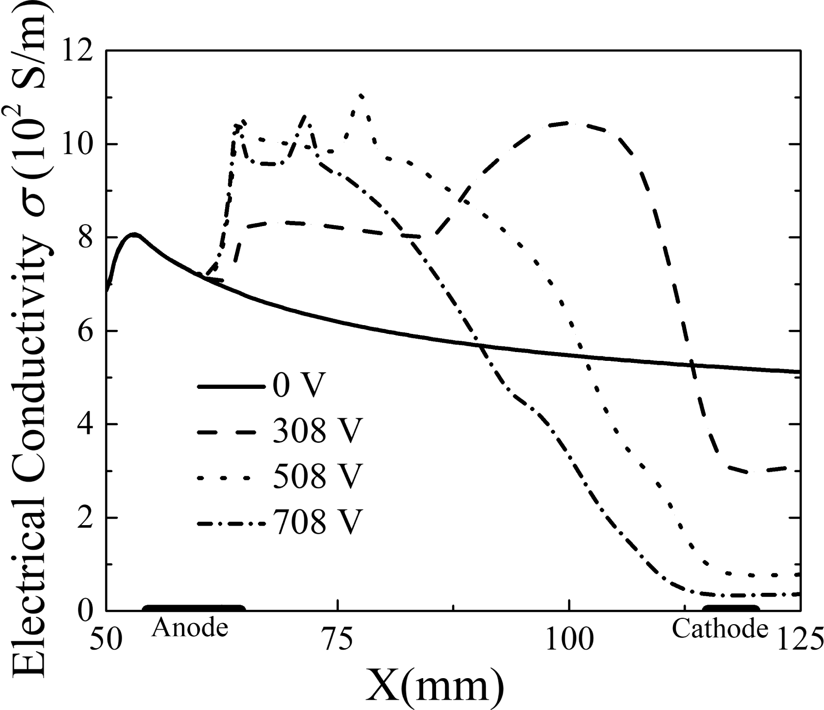
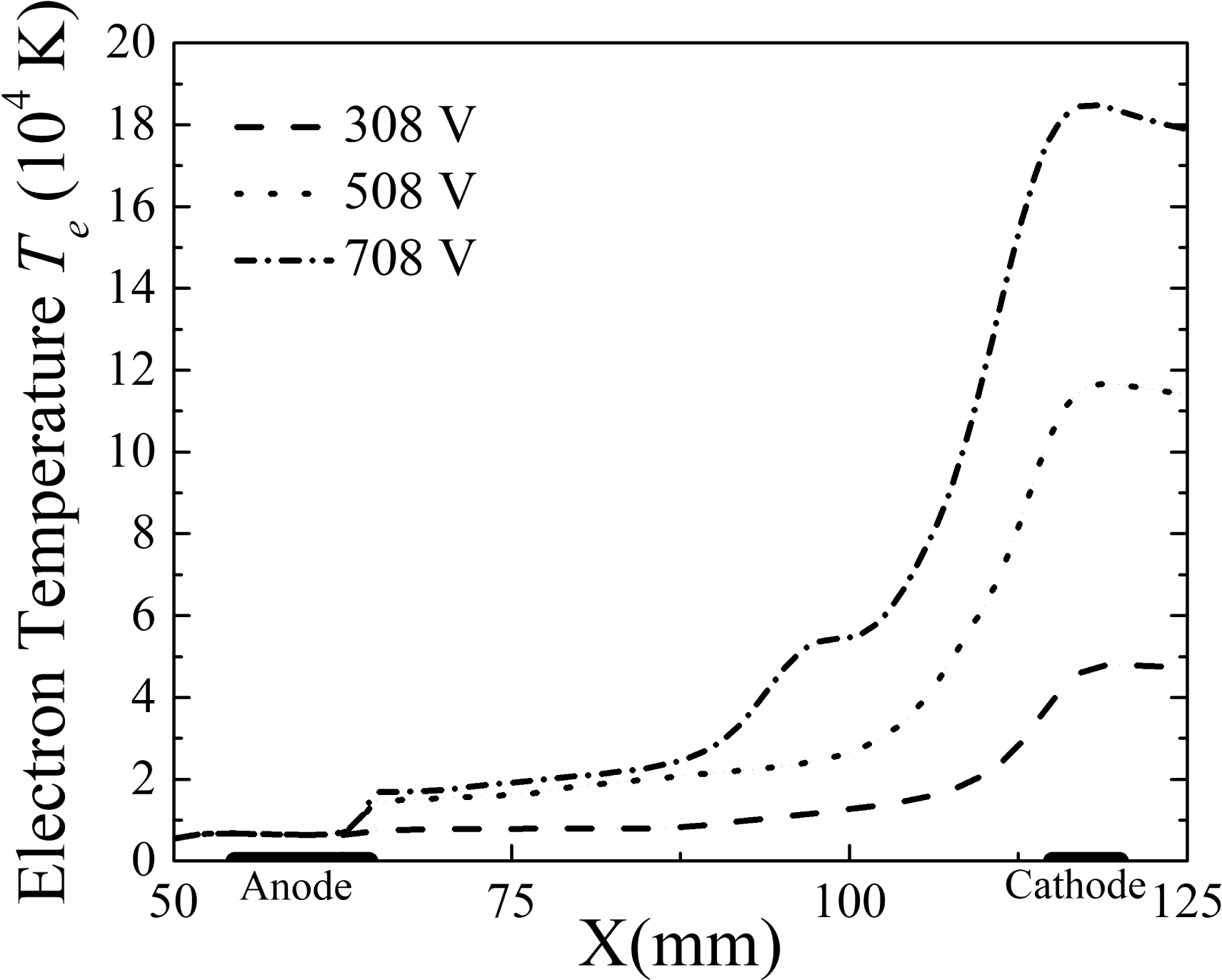
From a macroscopic perspective, the ionization degree of the plasma in this study was only approximately 0.4 %. When the external voltage was 0 V, the electron number density (figure 16) and average momentum transfer collision frequency (figure 17) decreased monotonically due to the increase in the velocity and lack of external energy input. As a result, the electrical conductivity of the 0 V case was relatively uniform (figure 18). As an important energy source for electron motion, Joule heating in the channel increased and resulted in a rise of the electron temperature, especially around the cathode area (figure 19). Consequently, the electrical conductivity increased due to the electron temperature increase, and the electron number density grew in the channel region from 65 to 105 mm when the external voltage was above 0 V. On the other hand, the electrical conductivity decreased from the location of 110 mm at 308 V, 102 mm at 508 V and 90 mm at 708 V due to the increase in the average momentum transfer collision frequency (figure 17).

Figure 16.

Distribution of electron number density.

Figure 17.

Distribution of average momentum transfer collision frequency.

Figure 18.

Distribution of electrical conductivity.

Figure 19.

Distribution of electron temperature.

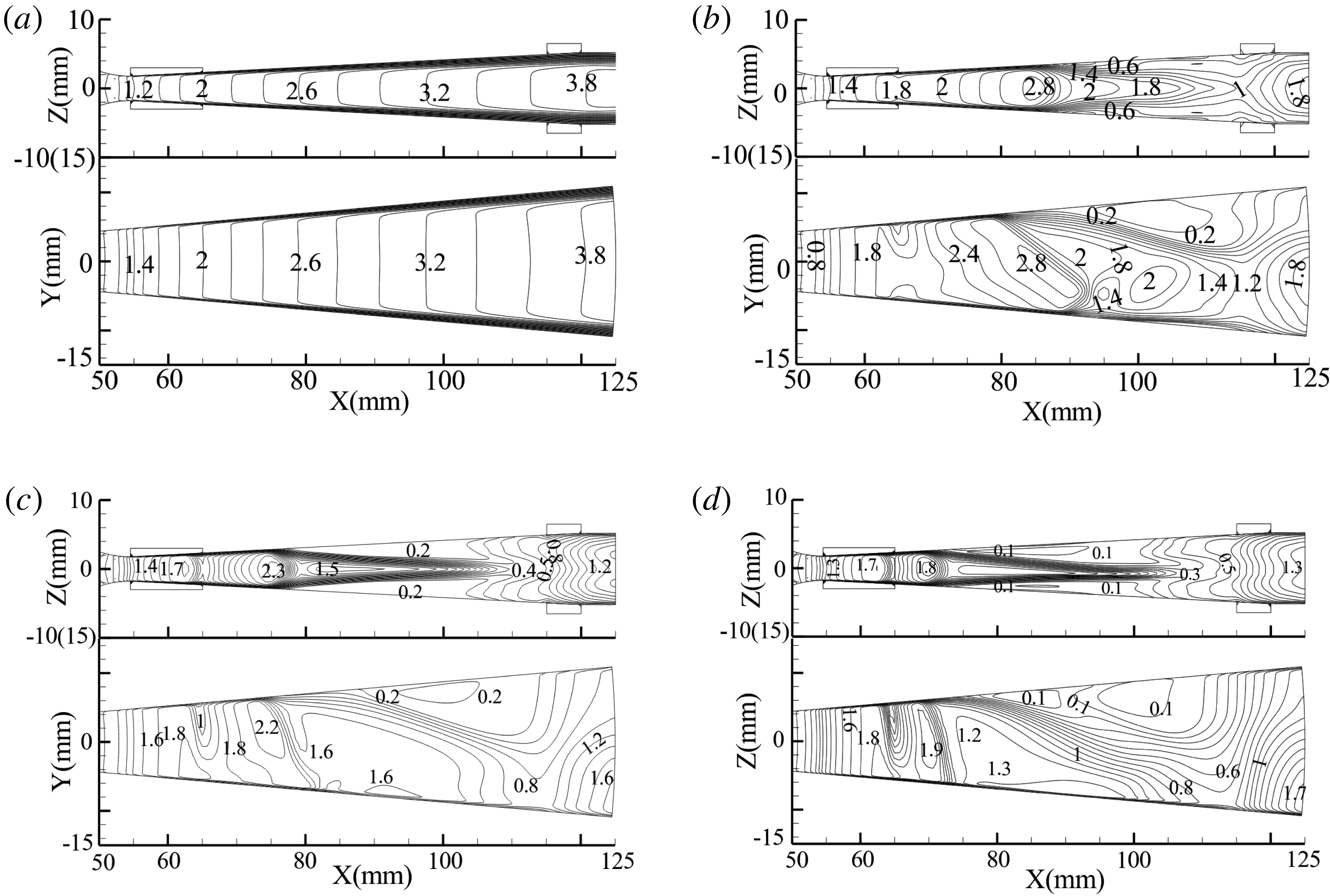
The Lorentz force in the $x$ direction ( $F_{x}=j_{y}B_{z}$ ) was produced by the interaction of the current density $j_{y}$ and magnetic field, whereas the Lorentz force in the $y$ direction ( $F_{y}=j_{x}B_{z}$ ) was formed by the interaction of the current density $j_{x}$ and the magnetic field. The Lorentz force $F_{x}$ accelerated the flow, whereas the Lorentz force $F_{y}$ deflected the flow (as shown in figure 20). Meanwhile, the Mach number decreased rapidly near the locations of 85 mm (308 V), 80 mm (508 V) and 75 mm (708 V). Shock waves, which occurred when the external potential was over 0 V, resulted in dramatic changes to the flow field, followed by sharp fluctuations in the electron number density and averaged momentum transfer collision frequency. The deflection of the flow led to the separation of boundary layers, which resulted in non-uniform distributions of the gas density and electric conductivity. The plasma was hindered by a reverse Lorentz force induced by the Hall potential near the cathode, and turbulence appeared in the flow field (80–125 mm for the 308 V case, 75–125 mm for the 508 V case and 70–125 mm for the 708 V case). For the 0 V external potential case with a low velocity and without energy input, the Mach number reached 3.8 at the exit as the static temperature decreased along the flow direction. With the voltages applied, the velocity is also affected by the gas temperature, especially the 708 V one in which the Joule heating is the strongest due to the maximum potential. Ultimately, the kinetic energy of the gas exhibits the highest increase due to the most significant increment in the gas temperature, as shown in figure 13.

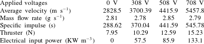
The acceleration effect was evident in the exit of the channels (80–100 mm) when the external potential increased from 308 to 708 V (figure 21). However, low Mach numbers appeared at the exit because the static temperature increased several times more than that of the 0 V case. Although the gas density decreased strongly at the exit when the external potential was growing, the mass flow rates of the final outflow were $2.81~\text{g}~\text{s}^{-1}$ (0 V), $2.78~\text{g}~\text{s}^{-1}$ (308 V), $2.85~\text{g}~\text{s}^{-1}$ (508 V) and $2.79~\text{g}~\text{s}^{-1}$ (708 V). In other words, the enlargement of the external potential could reach a relatively higher specific impulse. However, the channel structure must be further optimized to improve the gas flow distribution at the end of the channel.

Figure 20.

Contours of Mach number in XOZ and XOY cross-sections: (a) 0 V, (b) 308 V, (c) 508 V and (d) 708 V.

Figure 21.

Distribution of velocity $u_{x}$ .

Table 3.

Parameters of exit flow.

When the external potential grew, the thrust increased with a increase in the average velocity at the exit. Table 3 shows the results of the thrust and specific impulse from different simulations. The thrust in our study was larger than that of conventional Hall-effect propulsion. The specific impulse and the thrust were both the largest when the potential reached 708 V.