1 Introduction
Coherent Lagrangian vortices (Haller Reference Haller2015) are fluid masses enclosed by material boundaries that exhibit only moderate deformation under advection. Such vortices play a fundamental role in a number of transport and mixing processes. For instance, coherent mesoscale oceanic eddies are known to carry water over long distances, influencing global circulation and climate (Beal et al. Reference Beal, De Ruijter, Biastoch and Zahn2011).
Frame-invariant methods for the precise identification of coherent Lagrangian vortex boundaries are now available (Haller & Beron-Vera Reference Haller and Beron-Vera2013; Farazmand & Haller Reference Farazmand and Haller2016; Haller et al. Reference Haller, Hadjighasem, Farazmand and Huhn2016). These methods, as any Lagrangian approach, are intrinsically tied to a preselected finite time interval. Some material vortex boundaries lose their coherence immediately beyond their extraction times, while others remain coherent over much longer intervals (Beron-Vera et al. Reference Beron-Vera, Wang, Olascoaga, Goni and Haller2013; Haller & Beron-Vera Reference Haller and Beron-Vera2013; Wang, Beron-Vera & Olascoaga Reference Wang, Beron-Vera and Olascoaga2016). It is, therefore, of interest to identify a signature of long-lived Lagrangian vortices without an a priori knowledge of their time scale of existence.
The question we address in the present paper is the following: what instantaneous Eulerian features of a coherent Lagrangian vortex make it likely to persist over longer time intervals? This question is relevant, for instance, in environmental forecasting and decision making, as well as in assessing the life stage of coherent eddies that influence the general circulation in the ocean. Despite its importance, however, the question of Lagrangian vortex persistence has received little attention. Broadly used Eulerian vortex detection methods provide no direct answer, although the motivation for these Eulerian methods is often precisely the need to capture sustained material transport by vortices, see e.g. Chelton, Schlax & Samelson (Reference Chelton, Schlax and Samelson2011). Clearly, the future of advected water masses in an unsteady flow cannot be precisely predicted based on just present data. Reasons for this include unforeseeable future interactions with other vortices, and a priori unknown external forcing on the flow. The most one can hope for, therefore, is to forecast Lagrangian eddy persistence with high enough probability, assuming that these unpredictable effects do not arise.
To this end, we propose here a non-dimensional metric to assess the persistence of Eulerian vortices identified by elliptic objective Eulerian coherent structures (OECSs), as defined by Serra & Haller (Reference Serra and Haller2016). Such OECSs are closed curves with no short-term unevenness in their material deformation rates (zero short-term filamentation). The objectivity of OECSs ensures the frame invariance of the transport estimates they provide, while the non-dimensionality of the persistence metric introduced here will allow for a comparison of coexisting vortices of various sizes and times scales.
Our persistence metric is the ratio of the rotational coherence strength of an elliptic OECS to its material leakage. Eulerian vortices with high rotation rates and low material leakage will have high persistence metric values and will be seen to delineate regions of sustained material coherence. As a side result, we also derive an explicit formula for the material flux through an elliptic OECS. This technical result is generally applicable to estimating the deformation of limit cycles in a two-dimensional vector field under a change in the system parameters.
The method we devise here is purely kinematic, and hence is independent of the particular equation governing the underlying fluid. From a kinetic point of view, vortex lifetime is related to vortex instabilities, (see, e.g. Wang & Özgökmen (Reference Wang and Özgökmen2015) for a brief summary). A kinematic analysis is generally less specific than a kinetic one, yet tends to have a wider range of applicability and requires considerably less computational effort.
We illustrate our results on an unsteady satellite altimetry-based velocity field of the South Atlantic Ocean. Remarkably, we find that elliptic OECSs with high values of the persistence metric capture, with high probability, the signature of long-lived Lagrangian vortices. At the same time, the predictive power of customary Eulerian diagnostics, such as the Okubo–Weiss (OW) criterion (Okubo Reference Okubo1970; Weiss Reference Weiss1991), the potential vorticity (PV) and the potential vorticity gradient (
 $\unicode[STIX]{x1D735}$
PV) (Griffa et al.
Reference Griffa, Kirwan, Mariano, Özgökmen and Rossby2007), turns out to be substantially lower, showing correlations below 0.5 with the actual lifetime of Lagrangian eddies.
2 Set-up and notation
We consider an unsteady velocity field
 $v(x,t)$
defined in a spatial domain
 $U\subset \mathbb{R}^{2}$
over a finite time interval
 $[t_{0},t_{1}]$
. We recall the velocity gradient decomposition
 $$\begin{eqnarray}\unicode[STIX]{x1D735}v(x,t)=S(x,t)+W(x,t),\end{eqnarray}$$
where
 $S=(\unicode[STIX]{x1D735}v+\unicode[STIX]{x1D735}v^{\top })/2$
and
 $W=(\unicode[STIX]{x1D735}v-\unicode[STIX]{x1D735}v^{\top })/2$
are the rate-of-strain tensor and the spin tensor, respectively.
The spin tensor
 $W$
is skew-symmetric while
 $S$
is symmetric, with its eigenvalues
 $s_{i}(x)$
and eigenvectors
 $e_{i}(x)$
satisfying
 $$\begin{eqnarray}e_{2}Se_{i}=s_{i}e_{i},\quad |e_{i}|=1,\quad i=1,2;\quad s_{1}\leqslant s_{2},\quad e_{2}=Re_{1}=\left[\begin{array}{@{}cc@{}}0 & -1\\ 1 & 0\end{array}\right]e_{1}.\end{eqnarray}$$
Fluid particle trajectories generated by
 $v(x,t)$
are solutions of the differential equation
 ${\dot{x}}=v(x,t)$
, defining the flow map
 $$\begin{eqnarray}F_{t_{0}}^{t}(x_{0})=x(t;t_{0},x_{0}),\quad x_{0}\in U,\quad t\in [t_{0,}t_{1}],\end{eqnarray}$$
which maps initial particle positions
 $x_{0}$
at time
 $t_{0}$
to their time-
 $t$
positions,
 $x(t;t_{0},x_{0})$
. A key relationship between the flow map
 $F_{t_{0}}^{t}(x_{0})$
and
 $S(x,t)$
is obtained by considering the right Cauchy–Green strain tensor
 $$\begin{eqnarray}C_{t_{0}}^{t}=[\unicode[STIX]{x1D735}F_{t_{0}}^{t}]^{\text{T}}\unicode[STIX]{x1D735}F_{t_{0}}^{t},\end{eqnarray}$$
whose temporal Taylor expansion around the initial time can be computed as
 $$\begin{eqnarray}C_{t_{0}}^{t}(x_{0})=I+2S(x_{0},t_{0})(t-t_{0})+O(|t-t_{0}|^{2}).\end{eqnarray}$$
In other words, for small enough times, the leading-order Lagrangian deformation is governed by the Eulerian rate-of-strain tensor.
3 Vortices as elliptic OECSs
A typical set of fluid particles is subject to significant stretching under advection in an unsteady flow. Even in the limit of zero advection time, fluid elements generally experience considerable stretching rates. Motivated by (2.5), one may look for the Eulerian signatures of coherent material vortices as exceptional sets of fluid trajectories that defy this general trend. Specifically, Serra & Haller (Reference Serra and Haller2016) seek boundaries of Eulerian coherent vortices as closed instantaneous curves across which the averaged material stretching rate shows no leading-order variability.
Mathematically, this is equivalent to seeking closed curves
 $\unicode[STIX]{x1D6FE}$
whose
 $O(\unicode[STIX]{x1D716})$
perturbations show no
 $O(\unicode[STIX]{x1D716})$
variability in the averaged strain-rate functional
 $\dot{Q}_{t}(\unicode[STIX]{x1D6FE})$
, defined as
 $$\begin{eqnarray}\dot{Q}_{t}(\unicode[STIX]{x1D6FE})={\displaystyle \frac{1}{\unicode[STIX]{x1D70E}}}\oint _{\unicode[STIX]{x1D6FE}}{\displaystyle \frac{\langle x^{\prime }(s),S(x(s),t)x^{\prime }(s)\rangle }{\langle x^{\prime }(s),x^{\prime }(s)\rangle }}\,\text{d}s.\end{eqnarray}$$
Here
 $x(s)$
,
 $s\in [0,\unicode[STIX]{x1D70E}]$
, denotes the arclength parametrization of
 $\unicode[STIX]{x1D6FE}$
at time
 $t$
, and
 $x^{\prime }(s)$
denotes its local tangent vector. Stationary curves of
 $\dot{Q}_{t}(\unicode[STIX]{x1D6FE})$
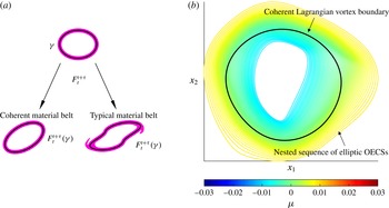
are cores of exceptional material belts showing perfect short-term coherence (figure 1
a). Serra & Haller (Reference Serra and Haller2016) show that closed stationary curves of
 $\dot{Q}_{t}(\unicode[STIX]{x1D6FE})$
are precisely the closed null-geodesics of a suitably defined Lorentzian metric. Along these curves, the tangential stretching rate
 $\unicode[STIX]{x1D707}$
is constant.
(a) A closed material curve
 $\unicode[STIX]{x1D6FE}$
(black) at time
 $t$
is advected by the flow into its later position
 $F_{t}^{t+\unicode[STIX]{x1D70F}}(\unicode[STIX]{x1D6FE})$
, with
 $\unicode[STIX]{x1D70F}\approx 0$
. The advected curve remains coherent if an initially uniform material belt (magenta) around it shows no leading-order variations in stretching rate. (b) Nested family of elliptic OECSs in a flow example, analysed in more detail in § 6, for different values of
 $\unicode[STIX]{x1D707}$
(in colour). The elliptic OECS family fills a region that also turns out to contain a persistent Lagrangian vortex in this example (Haller & Beron-Vera Reference Haller and Beron-Vera2013).

The closed stationary curves of
 $\dot{Q}_{t}(\unicode[STIX]{x1D6FE})$
turn out to be computable as limit cycles of the direction field family
 $$\begin{eqnarray}x^{\prime }=\unicode[STIX]{x1D712}_{\unicode[STIX]{x1D707}}^{\pm }(x),\quad \unicode[STIX]{x1D712}_{\unicode[STIX]{x1D707}}^{\pm }(x)=\sqrt{{\displaystyle \frac{s_{2}(x)-\unicode[STIX]{x1D707}}{s_{2}(x)-s_{1}(x)}}}e_{1}(x)\pm \sqrt{{\displaystyle \frac{\unicode[STIX]{x1D707}-s_{1}(x)}{s_{2}(x)-s_{1}(x)}}}e_{2}(x),\end{eqnarray}$$
within the domain
 $U_{\unicode[STIX]{x1D707}}\subset U$
defined as
 $$\begin{eqnarray}U_{\unicode[STIX]{x1D707}}=\{x\in U\mid s_{2}-s_{1}\neq 0,s_{1}\leqslant \unicode[STIX]{x1D707}\leqslant s_{2}\}.\end{eqnarray}$$
The direction field family (3.2) depends on the choice of the sign parameter
 $\pm$
, as well as on the parameter
 $\unicode[STIX]{x1D707}\in \mathbb{R}$
. We define elliptic OECSs as limit cycles of (3.2) for each value of the parameter
 $\unicode[STIX]{x1D707}\approx 0$
. The
 $\unicode[STIX]{x1D707}=0$
member of this one-parameter family of nested curves represents a perfect instantaneously coherent vortex boundary (Serra & Haller Reference Serra and Haller2016). Such a closed curve is highly atypical, exhibiting no instantaneous stretching rate.
Members of limit cycles families of
 $\unicode[STIX]{x1D712}_{\unicode[STIX]{x1D707}}^{\pm }$
cannot intersect. Each limit cycle either grows or shrinks under changes in
 $\unicode[STIX]{x1D707}$
, forming a smooth annular belt of non-intersecting loops (see Serra & Haller (Reference Serra and Haller2016) for details). This annular Eulerian belt often surrounds a persistent Lagrangian vortex boundary, as shown in figure 1(b) for a flow example analysed in more detail in § 6.
4 Material flux through elliptic OECSs
In this section, we derive an explicit formula for the material flux through an elliptic OECS to quantify the degree to which the OECS is Lagrangian. As a byproduct, we obtain an expression for the short-term continuation of elliptic OECSs under varying time.
Let
 $\unicode[STIX]{x1D6FE}(t)$
be a time-varying, closed curve family parametrized by a function
 $x(s,t)$
. The pointwise instantaneous material flux density through
 $\unicode[STIX]{x1D6FE}(t)$
is then given by
 $$\begin{eqnarray}\displaystyle \unicode[STIX]{x1D711}(x(s,t),t) & = & \displaystyle \left\langle v(x(s,t),t)-\frac{\text{d}}{\text{d}t}x(s,t),n(x(s,t),t)\right\rangle \nonumber\\ \displaystyle & = & \displaystyle \langle v(x(s,t),t),n(x(s,t),t)\rangle -\left[\frac{\text{d}}{\text{d}t}x(s,t)\right]^{\bot },\end{eqnarray}$$
i.e. by the curve-normal projection
 $\langle \cdot ,n(x(s,t),t)\rangle$
of the Lagrangian velocity
 $v(x(s,t),t)$
of a trajectory relative to the velocity of
 $\unicode[STIX]{x1D6FE}(t)$
.
In our context,
 $x(s,t)$
represents a limit cycle of the ordinary differential equation (ODE) (3.2), thus we have
 $n(x(s,t),t)=[\unicode[STIX]{x1D712}_{\unicode[STIX]{x1D707}}^{\pm }(x(s,t),t)]^{\bot }=R\unicode[STIX]{x1D712}_{\unicode[STIX]{x1D707}}^{\pm }(x(s,t),t)$
. In appendix A, we derive and solve an ODE for the unknown term
 $[(\text{d}/\text{d}t)x(s,t)]^{\bot }$
in (4.1), obtaining the final formula
 $$\begin{eqnarray}\left[\frac{\text{d}}{\text{d}t}x(s,t)\right]^{\bot }=\unicode[STIX]{x1D6F7}_{0}^{s}(t)\left[\frac{\text{d}}{\text{d}t}x(0,t)\right]^{\bot }+\unicode[STIX]{x1D6F1}(s,t),\quad \unicode[STIX]{x1D6F1}(s,t):=\unicode[STIX]{x1D6F7}_{0}^{s}(t)\int _{0}^{s}(\unicode[STIX]{x1D6F7}_{0}^{\unicode[STIX]{x1D717}}(t))^{-1}\tilde{c}(\unicode[STIX]{x1D717},t)\,\text{d}\unicode[STIX]{x1D717},\end{eqnarray}$$
with
 $\unicode[STIX]{x1D6F7}_{0}^{s}(t)$
denoting the matrix
 $$\begin{eqnarray}\unicode[STIX]{x1D6F7}_{0}^{s}(t)=\left[\begin{array}{@{}cc@{}}1 & \displaystyle \int _{0}^{s}\exp \left(\displaystyle \int _{0}^{\unicode[STIX]{x1D717}}\unicode[STIX]{x1D735}\boldsymbol{\cdot }\unicode[STIX]{x1D712}_{\unicode[STIX]{x1D707}}^{\pm }(x(\unicode[STIX]{x1D717},t),t)\,\text{d}\unicode[STIX]{x1D717}\right)\unicode[STIX]{x1D705}(x(\unicode[STIX]{x1D717},t))\,\text{d}\unicode[STIX]{x1D717}\\ 0 & \exp \left(\displaystyle \int _{0}^{s}\unicode[STIX]{x1D735}\boldsymbol{\cdot }\unicode[STIX]{x1D712}_{\unicode[STIX]{x1D707}}^{\pm }(x(\unicode[STIX]{x1D717},t),t)\,\text{d}\unicode[STIX]{x1D717}\right)\end{array}\right],\end{eqnarray}$$
and
 $$\begin{eqnarray}\left.\begin{array}{@{}c@{}}\tilde{c}(s,t)=[0,\unicode[STIX]{x1D713}(x(s,t),t)]^{\top },\\ \unicode[STIX]{x1D713}(x(s,t),t)={\displaystyle \frac{-\langle \unicode[STIX]{x1D712}_{\unicode[STIX]{x1D707}}^{\pm }(s,t),\unicode[STIX]{x2202}_{t}S(s,t)\unicode[STIX]{x1D712}_{\unicode[STIX]{x1D707}}^{\pm }(s,t)\rangle }{2\langle \unicode[STIX]{x1D712}_{\unicode[STIX]{x1D707}}^{\pm }(s,t),S(s,t)\unicode[STIX]{x1D712}_{\unicode[STIX]{x1D707}}^{\pm }(s,t)^{\bot }\rangle }},\\ \unicode[STIX]{x1D705}(x(s,t))=\langle \unicode[STIX]{x1D735}\unicode[STIX]{x1D712}_{\unicode[STIX]{x1D707}}^{\pm }(s,t)\unicode[STIX]{x1D712}_{\unicode[STIX]{x1D707}}^{\pm }(s,t),R\unicode[STIX]{x1D712}_{\unicode[STIX]{x1D707}}^{\pm }(s,t)\rangle .\end{array}\right\}\end{eqnarray}$$
Note that
 $\unicode[STIX]{x1D705}$
represents the pointwise curvature along the elliptic OECS with respect to the normal vector defined as
 $[\unicode[STIX]{x1D712}_{\unicode[STIX]{x1D707}}^{\pm }]^{\bot }=R\unicode[STIX]{x1D712}_{\unicode[STIX]{x1D707}}^{\pm }$
.
In appendix A, we also derive the following equation for the correct initial condition of
 $[(\text{d}/\text{d}t)x(s,t)]^{\bot }$
:
 $$\begin{eqnarray}\left[\frac{\text{d}}{\text{d}t}x(0,t)\right]^{\bot }=\frac{\langle \unicode[STIX]{x1D6F1}(\unicode[STIX]{x1D70E},t),d\rangle }{1-\unicode[STIX]{x1D70C}_{2}(t)},\quad \unicode[STIX]{x1D70C}_{2}(t)=\exp \left(\displaystyle \int _{0}^{\unicode[STIX]{x1D70E}}\unicode[STIX]{x1D735}\boldsymbol{\cdot }\unicode[STIX]{x1D712}_{\unicode[STIX]{x1D707}}^{\pm }(x(\unicode[STIX]{x1D717},t),t)\,\text{d}\unicode[STIX]{x1D717}\right)\!,\quad d:=\left[\begin{array}{@{}c@{}}0\\ 1\end{array}\right]\!.\quad\end{eqnarray}$$
This initial condition represents the ratio between the magnitude of the perturbation needed to destroy the limit cycle due to the unsteadiness of the flow, and the strength of the hyperbolicity of the limit cycle. For steady flows, we have
 $\unicode[STIX]{x1D6F1}^{\bot }(s,t)=0$
since
 $\tilde{c}(s,t)=0$
. In that case, the robustness of the limit cycle is determined by
 $\unicode[STIX]{x1D70C}_{2}(t)\equiv \unicode[STIX]{x1D70C}_{2}=\text{const.}$
, without any time dependence.
Once
 $[(\text{d}/\text{d}t)x(0,t)]^{\bot }$
is known, we evaluate the pointwise flux density introduced in (4.1). For a counterclockwise parametrization of
 $\unicode[STIX]{x1D6FE}(t)$
, and for our definition of
 $[\unicode[STIX]{x1D712}_{\unicode[STIX]{x1D707}}^{\pm }]^{\bot }$
, positive values of
 $\unicode[STIX]{x1D711}(x(s,t),t)$
represents inward material flux.
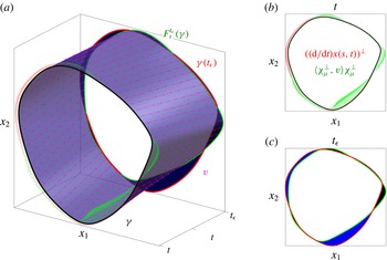
Figure 2(a) illustrates an elliptic OECS
 $\unicode[STIX]{x1D6FE}(t)$
(black) at time
 $t$
, for a fixed value of
 $\unicode[STIX]{x1D707}$
, with its advected image over the time window
 $[t,t_{\unicode[STIX]{x1D716}}]$
in the extended phase space of position and time. Figure 2(b,c) shows the initial and final time slices of figure 2(a). The materially advected image of
 $\unicode[STIX]{x1D6FE}$
at time
 $t_{\unicode[STIX]{x1D716}}$
,
 $F_{t}^{t_{\unicode[STIX]{x1D716}}}(\unicode[STIX]{x1D6FE})$
, is shown in green while the elliptic OECS
 $\unicode[STIX]{x1D6FE}(t_{\unicode[STIX]{x1D716}})$
computed at time
 $t_{\unicode[STIX]{x1D716}}$
, is shown in red. Figure 2(a,b) shows the instantaneous pointwise material flux density through
 $\unicode[STIX]{x1D6FE}(t)$
, given by the difference between the flow velocity normal to the curve (green arrows) and the corresponding continuation velocity (red arrows). Given formula (4.1), the total instantaneous material flux across
 $\unicode[STIX]{x1D6FE}(t)$
is
 $$\begin{eqnarray}\unicode[STIX]{x1D711}_{\unicode[STIX]{x1D6FE}(t)}=\oint _{\unicode[STIX]{x1D6FE}(t)}\unicode[STIX]{x1D711}(x(s,t),t)\,\text{d}s,\end{eqnarray}$$
with
 $$\begin{eqnarray}\left.\begin{array}{@{}c@{}}\unicode[STIX]{x1D711}(x(s,t),t)=\langle v(x(s,t),t),[\unicode[STIX]{x1D712}_{\unicode[STIX]{x1D707}}^{\pm }]^{\bot }(x(s,t),t)\rangle -\left\langle \unicode[STIX]{x1D6F7}_{0}^{s}(t)\left[{\displaystyle \frac{\text{d}}{\text{d}t}}x(0,t)\right]^{\bot }+\unicode[STIX]{x1D6F1}(s,t),d\right\rangle ,\\ \left[{\displaystyle \frac{\text{d}}{\text{d}t}}x(0,t)\right]^{\bot }={\displaystyle \frac{\langle \unicode[STIX]{x1D6F1}(\unicode[STIX]{x1D70E},t),d\rangle }{1-\exp \left(\displaystyle \int _{0}^{\unicode[STIX]{x1D70E}}\unicode[STIX]{x1D735}\boldsymbol{\cdot }\unicode[STIX]{x1D712}_{\unicode[STIX]{x1D707}}^{\pm }(x(\unicode[STIX]{x1D717},t),t)\,\text{d}\unicode[STIX]{x1D717}\right)}}.\end{array}\right\}\end{eqnarray}$$
The instantaneous total material flux
 $\unicode[STIX]{x1D711}_{\unicode[STIX]{x1D6FE}(t)}$
, multiplied by
 $\unicode[STIX]{x1D716}\unicode[STIX]{x0394}t$
, approximates the actual material flux given by the inward (blue) area minus the outward (black) area shown in figure 2(c).
(a) Initial elliptic OECS
 $\unicode[STIX]{x1D6FE}$
(black) and its advected image under the flow in the extended phase space over
 $[t,t_{\unicode[STIX]{x1D716}}]$
, where
 $t_{\unicode[STIX]{x1D716}}=t+\unicode[STIX]{x1D716}\unicode[STIX]{x0394}t$
. At time
 $t$
, the flow velocity perpendicular to the curve and the corresponding elliptic OECS velocity are reported by the green and red arrows, respectively. At time
 $t_{\unicode[STIX]{x1D716}}$
, the advected image,
 $F_{t}^{t_{\unicode[STIX]{x1D716}}}(\unicode[STIX]{x1D6FE})$
, is shown in green while the recomputed elliptic OECS
 $\unicode[STIX]{x1D6FE}(t_{\unicode[STIX]{x1D716}})$
in red. (b) Slice of (a) at time
 $t$
. (c) Slice of (a) at time
 $t_{\unicode[STIX]{x1D716}}$
. The blue and black areas represent the actual inward and outward material flux across
 $\unicode[STIX]{x1D6FE}$
over
 $[t,t_{\unicode[STIX]{x1D716}}]$
, respectively.

5 Persistence metric for elliptic OECSs
We now propose an instantaneous, non-dimensional and objective metric that classifies elliptic OECSs based on their expected persistence in time. We first define the two ingredients needed for this metric: the rotational coherence and the relative material leakage.
Definition 1. The rotational coherence of an elliptic OECS
 $\unicode[STIX]{x1D6FE}(t)$
is
 $$\begin{eqnarray}\unicode[STIX]{x1D714}_{\unicode[STIX]{x1D6FE}}(t):={\displaystyle \frac{\left|\displaystyle \int _{A_{\unicode[STIX]{x1D6FE}(t)}}[\unicode[STIX]{x1D714}(x,t)-\overline{\unicode[STIX]{x1D714}}(t)]\,\text{d}A\right|}{A_{\unicode[STIX]{x1D6FE}(t)}}},\end{eqnarray}$$
where
 $\unicode[STIX]{x1D714}(x,t)$
denotes the vorticity,
 $A_{\unicode[STIX]{x1D6FE}(t)}$
is the area enclosed by
 $\unicode[STIX]{x1D6FE}(t)$
and
 $$\begin{eqnarray}\overline{\unicode[STIX]{x1D714}}(t)={\displaystyle \frac{\displaystyle \int _{A_{\unicode[STIX]{x2202}U}}\unicode[STIX]{x1D714}(x,t)\,\text{d}A}{A_{\unicode[STIX]{x2202}U}}}\end{eqnarray}$$
is the mean spatial vorticity over the domain
 $U$
with boundary
 $\unicode[STIX]{x2202}U$
.
The rotational coherence
 $\unicode[STIX]{x1D714}_{\unicode[STIX]{x1D6FE}}$
represents the normed mean vorticity deviation within
 $\unicode[STIX]{x1D6FE}(t)$
, inspired by related quantities defined in Haller et al. (Reference Haller, Hadjighasem, Farazmand and Huhn2016). Specifically, the rotational coherence measures the strength of a vortical structure arising from its rotational speed. The classic measure of vortex strength, also called circulation (Batchelor Reference Batchelor2000), relies solely on the vorticity
 $\unicode[STIX]{x1D714}(x,t)$
, and is therefore frame dependent. The rotational coherence
 $\unicode[STIX]{x1D714}_{\unicode[STIX]{x1D6FE}}$
, instead, involves the vorticity deviation, which is frame independent (appendix B). The rotational coherence
 $\unicode[STIX]{x1D714}_{\unicode[STIX]{x1D6FE}}(t)$
depends on the size of the domain, and should be computed on a large enough domain so that the averaged vorticity is representative of the overall mean rotation of the flow. In geophysical flows, this mean rotation is expected to be zero, which is confirmed by our calculations in § 6. Elliptic OECSs with high rotational coherence are shielded by locally high levels of shear, and hence are expected to persist in time.
Definition 2. The relative material leakage of an elliptic OECS
 $\unicode[STIX]{x1D6FE}(t)$
is
 $$\begin{eqnarray}\unicode[STIX]{x1D6E4}_{\unicode[STIX]{x1D6FE}}(t):={\displaystyle \frac{\displaystyle \oint _{\unicode[STIX]{x1D6FE}(t)}|\unicode[STIX]{x1D711}(x(s,t),t)|\,\text{d}s}{A_{\unicode[STIX]{x1D6FE}(t)}}}.\end{eqnarray}$$
The relative material leakage measures the rate of material area leaking out of
 $\unicode[STIX]{x1D6FE}(t)$
due to its non-Lagrangian evolution, divided by the initial area of
 $\unicode[STIX]{x1D6FE}(t)$
. A
 $\unicode[STIX]{x1D6FE}(t)$
with low
 $\unicode[STIX]{x1D6E4}_{\unicode[STIX]{x1D6FE}}(t)$
identifies an exceptional curve that exhibits low inhomogeneity in its stretching rates both in its initial position and in its short-term advected position. The absolute value in (5.3) prevents the cancellation of opposite-sign material flux contributions. Note that both
 $\unicode[STIX]{x1D714}_{\unicode[STIX]{x1D6FE}}$
and
 $\unicode[STIX]{x1D6E4}_{\unicode[STIX]{x1D6FE}}$
have the dimension
 $(\text{time}^{-1})$
.
We expect elliptic OECSs with high rotational coherence and low material leakage to be the best candidate locations for Lagrangian vortices. To this end, we define the persistence metric of an elliptic OECS as the following objective, non-dimensional quantity:
Definition 3. The persistence metric of elliptic OECS
 $\unicode[STIX]{x1D6FE}(t)$
is
 $$\begin{eqnarray}\unicode[STIX]{x1D6E9}_{\unicode[STIX]{x1D6FE}}(t):={\displaystyle \frac{\mathit{rotational~coherence}}{\mathit{relative~material~leakage}}}={\displaystyle \frac{\unicode[STIX]{x1D714}_{\unicode[STIX]{x1D6FE}}(t)}{\unicode[STIX]{x1D6E4}_{\unicode[STIX]{x1D6FE}}(t)}}={\displaystyle \frac{\left|\displaystyle \int _{A_{\unicode[STIX]{x1D6FE}(t)}}[\unicode[STIX]{x1D714}(x,t)-\overline{\unicode[STIX]{x1D714}}(t)]\,\text{d}A\right|}{\displaystyle \oint _{\unicode[STIX]{x1D6FE}(t)}|\unicode[STIX]{x1D711}(x(s,t),t)|\,\text{d}s}}.\end{eqnarray}$$
The non-dimensional nature of
 $\unicode[STIX]{x1D6E9}_{\unicode[STIX]{x1D6FE}}$
is immediate from (5.4), while its frame-invariance follows from the objectivity of the scalar quantities involved in its definition (cf. appendix B). The non-dimensionality of
 $\unicode[STIX]{x1D6E9}_{\unicode[STIX]{x1D6FE}}$
allows us to characterize the persistence of vortices regardless of the their spatial and temporal scales, which are often abundant and unknown. The objectivity of
 $\unicode[STIX]{x1D6E9}_{\unicode[STIX]{x1D6FE}}$
ensures a persistence assessment independent of the frame of reference.
In case of zero relative material leakage, we have
 $\unicode[STIX]{x1D6E9}_{\unicode[STIX]{x1D6FE}}=\infty$
, as indeed desired for a perfectly material elliptic OECSs. In this rare case,
 $F_{t}^{t_{\unicode[STIX]{x1D716}}}(\unicode[STIX]{x1D6FE}(t))=\unicode[STIX]{x1D6FE}(t_{\unicode[STIX]{x1D716}})$
and hence the green and the red curves in figure 2(c) coincide. In the case of irrotational flows, the relative material leakage of elliptic OECSs is the only necessary quantity to address eddy persistence over time. For these flows, the persistence metric should simply be the inverse of the relative material leakage.
In appendix C, we summarize the numerical algorithms for the identification of likely long-lived Lagrangian vortices from their objective Eulerian features. Specifically, Algorithm 1 summarizes the computation of elliptic OECSs and Algorithm 2 describes the computation of the corresponding persistence metric
 $\unicode[STIX]{x1D6E9}_{\unicode[STIX]{x1D6FE}}$
.
6 Example: forecasting persistent Lagrangian vortices in satellite-derived ocean velocity data
We apply our OECS-based vortex-coherence forecasting scheme to a two-dimensional unsteady ocean dataset obtained from AVISO satellite altimetry measurements (http://www.aviso.oceanobs.com). The domain of interest is the Agulhas leakage in the Southern Atlantic Ocean bounded by longitudes
 $[17^{\circ }\text{W},7^{\circ }\text{E}]$
and latitudes
 $[38^{\circ }\text{S},22^{\circ }\text{S}]$
. The Agulhas Current is a narrow western boundary current of the southwest Indian Ocean, whose interaction with the strong Antarctic Circumpolar Current gives rise to Agulhas rings, the largest mesoscale eddies in the ocean.
Agulhas rings are considered important in the global circulation due to the large amount of water they carry over considerable distances (Beal et al.
Reference Beal, De Ruijter, Biastoch and Zahn2011). For comparison with earlier Lagrangian analysis (Haller & Beron-Vera Reference Haller and Beron-Vera2013), we consider the same initial time
 $t=24~\text{November}~2006$
and a similar but slightly larger spatial domain. For more detail on the dataset and the numerical method, see appendices C and D.
As mentioned earlier, the OW parameter
 $$\begin{eqnarray}\text{OW}(x,t)=s_{2}^{2}(x,t)-\unicode[STIX]{x1D714}^{2}(x,t),\end{eqnarray}$$
is a frequently used indicator of instantaneous ellipticity in unsteady fluid flows (Okubo Reference Okubo1970; Weiss Reference Weiss1991). Spatial domains with OW
 $(x,t)<0$
(rotation prevailing over strain) are generally considered vortical. The OW parameter is not objective (the vorticity term will change under rotations), and hence no objective threshold level can be defined for this scalar field to identify vortices unambiguously. This ambiguity significantly impacts the overall number and geometry of the vortical structures inferred from the OW parameter (appendix E). Among other applications, OW has been used to study eddies in the Gulf of Alaska (Henson & Thomas Reference Henson and Thomas2008), in the Mediterranean Sea (Isern-Fontanet, García-Ladona & Font Reference Isern-Fontanet, García-Ladona and Font2003; Isern-Fontanet et al.
Reference Isern-Fontanet, Font, García-Ladona, Emelianov, Millot and Taupier-Letage2004; Isern-Fontanet, García-Ladona & Font Reference Isern-Fontanet, García-Ladona and Font2006), in the Tasman Sea (Waugh, Abraham & Bowen Reference Waugh, Abraham and Bowen2006) and in the global ocean (Chelton et al.
Reference Chelton, Schlax, Samelson and De Szoeke2007).
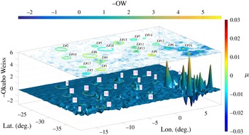
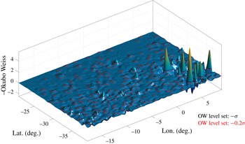
In figure 3, we show elliptic OECSs with the highest persistence metric
 $\unicode[STIX]{x1D6E9}_{\unicode[STIX]{x1D6FE}}$
for each vortical region, on a surface representing the negative OW parameter. The plane of the figure also shows the level curves of the OW parameter. The black numbers in figure 3 label the different vortical structures, while the magenta numbers classify them in decreasing order of
 $\unicode[STIX]{x1D6E9}_{\unicode[STIX]{x1D6FE}}$
. We find elliptic OECSs in locations of the flow where the OW parameter is close to zero and hence signals no vortices (see, e.g.
 $E\#7$
,
 $E\#8$
,
 $E\#18$
). In contrast, close to the tip of Africa, OW signals several strong vortical regions, even though we only detect two belts of elliptic OECSs (
 $E\#6$
,
 $E\#16$
).
Elliptic OECSs with the highest persistence metric
 $\unicode[STIX]{x1D6E9}_{\unicode[STIX]{x1D6FE}}$
on a surface representing the negative OW
 $\;(\text{day}^{-1})$
parameter (horizontal colour bar or
 $z$
-axis). The colour of elliptic OECSs represents the corresponding stretching rate value
 $\unicode[STIX]{x1D707}\;(\text{day}^{-1})$
(right colour bar). Black numbers identify different vortical regions detected by elliptic OECSs. In magenta, the classification of the most persistent vortical regions in decreasing order of
 $\unicode[STIX]{x1D6E9}_{\unicode[STIX]{x1D6FE}}$
.

To assess these discrepancies between the OW parameter and our persistence metric
 $\unicode[STIX]{x1D6E9}_{\unicode[STIX]{x1D6FE}}$
, we compare the coherence strength suggested by
 $\unicode[STIX]{x1D6E9}_{\unicode[STIX]{x1D6FE}}$
to the actual lifetime of Lagrangian vortices computed over a time window of four months with initial time
 $t=24~\text{November}~2006$
. We compute the Lagrangian lifetime of elliptic OECSs as the maximum integration time for which non-filamenting Lagrangian vortices (cf. Haller & Beron-Vera Reference Haller and Beron-Vera2013) exist nearby. Specifically, using the automated detection scheme of Karrasch, Huhn & Haller (Reference Karrasch, Huhn and Haller2015), we compute coherent Lagrangian eddies for the discrete set of integration times:
 $T=[7,15,30,60,90,120]$
days. For each such integration time, there are several vortex boundaries with lifetime
 $T$
. The Lagrangian lifetime of an elliptic OECSs is then the largest
 $T$
from this sequence for which there exists a nearby Lagrangian eddy. We consider a Lagrangian eddy to be near to an elliptic OECS if it is contained within a circle of radius
 $3^{\circ }$
(
 ${\sim}1.5$
times the radius of a mesoscale eddy) centred at the elliptic OECS. We do not consider larger
 $T$
due to the sensitivity of numerical errors with respect to increasing integration times.
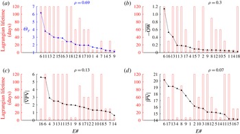
(a) Values of the persistence metric
 $\unicode[STIX]{x1D6E9}_{\unicode[STIX]{x1D6FE}}$
(blue) for the different vortical regions identified by elliptic OECSs compared with their Lagrangian lifetime (red). (b–d) Spatial average of
 $-$
OW
 $\;(\text{day}^{-1})$
,
 $|\unicode[STIX]{x1D735}$
PV
 $|\;((\text{deg}\cdot \text{day})^{-1})$
and
 $|$
PV
 $|\;(\text{day}^{-1})$
within elliptic OECSs compared with their Lagrangian lifetime (red). The parameter
 $\unicode[STIX]{x1D70C}$
indicates the correlation coefficient between the instantaneous prediction given by each metric and the actual Lagrangian lifetime of the underlying vortical region.

Figure 4(a) shows the
 $\unicode[STIX]{x1D6E9}_{\unicode[STIX]{x1D6FE}}$
values (blue) associated with each vortical region
 $(E\#i)$
in descending order of
 $\unicode[STIX]{x1D6E9}_{\unicode[STIX]{x1D6FE}}$
. Figure 4(b–d), in contrast, shows alternative instantaneous metrics, such as the average of
 $-$
OW,
 $|\unicode[STIX]{x1D735}$
PV
 $|$
and
 $|$
PV
 $|$
, respectively, within the elliptic OECSs shown in figure 3. For this dataset, we compute PV as in Early, Samelson & Chelton (Reference Early, Samelson and Chelton2011) (cf. appendix F). The actual Lagrangian lifetime of the underlying vortical regions is shown in red in all the plots, along with its correlations with the different instantaneous metrics.
The instantaneous persistence metric
 $\unicode[STIX]{x1D6E9}_{\unicode[STIX]{x1D6FE}}$
shows a distinct correlation (
 $\unicode[STIX]{x1D70C}\approx 0.7$
) with the lifetime of long-lived Lagrangian eddies in our study domain. This includes eddies
 $\#6,\#11,\#13,\#15,\#18,\#8,\#2$
and
 $\#3$
, previously identified as exceptionally coherent Lagrangian eddy regions in Haller & Beron-Vera (Reference Haller and Beron-Vera2013) and Karrasch et al. (Reference Karrasch, Huhn and Haller2015). Figure 4(a) shows that out of the ten elliptic OECSs with the highest
 $\unicode[STIX]{x1D6E9}_{\unicode[STIX]{x1D6FE}}$
values, eight are long-lived Lagrangian vortices.
Instantaneous forecasting tools, however, cannot predict unforeseeable future interactions with other vortices, or a priori unknown external forcing on the flow. This explains the weaker forecast for some eddies compared to the others e.g. eddies
 $\#16$
and
 $\#8$
in figure 4(a). Updating
 $\unicode[STIX]{x1D6E9}_{\unicode[STIX]{x1D6FE}}$
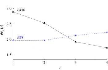
in time, however, we obtain more robust predictive information. As an example, in figure 5 we show the persistence metric of eddies
 $\#16$
and
 $\#8$
at four consecutive times one week apart from each other, with
 $t=1$
referring to the current time
 $24~\text{November}~2006$
. While
 $\unicode[STIX]{x1D6E9}_{\unicode[STIX]{x1D6FE}}$
of
 $E\#16$
decreases in time,
 $\unicode[STIX]{x1D6E9}_{\unicode[STIX]{x1D6FE}}$
of
 $E\#8$
slightly increase in time, in agreement with their actual lifetimes. We also note that
 $\unicode[STIX]{x1D6E9}_{\unicode[STIX]{x1D6FE}}$
of eddy
 $\#6$
(cf. figure 4
a) is high compared with the other eddies. Indeed, the elliptic Lagrangian coherent structures (LCSs) corresponding to eddy 6, constructed from four months of data, shows no sign of disintegration up to one year and a half, consistent with the findings of Beron-Vera et al. (Reference Beron-Vera, Wang, Olascoaga, Goni and Haller2013).
Persistence metric of eddies
 $E\#16$
and
 $E\#8$
recomputed at four consecutive times one week apart from each other. The initial time
 $t=1$
refers the current time
 $24~\text{November}~2006$
.

At the same time, figure 4(b–d), reveals a global weak predictive power for other instantaneous Eulerian diagnostics, each of which has significantly lower correlation with the Lagrangian lifetime of eddies. Figure 4(b,c) shows that long-lived mesoscale eddies, such as
 $E\#2$
and
 $E\#18$
, have surprisingly weak signatures in the OW and
 $|\unicode[STIX]{x1D735}$
PV
 $|$
fields, while the vortex
 $\#16$
, which has a relatively low Lagrangian lifetime, has the strongest signature in these two fields. The correlation coefficients of these diagnostics is even lower if the candidate vortical regions are identified from the usual ad hoc threshold values for these methods, instead of elliptic OECSs.
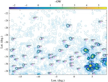
As an example, figure 7 (cf. appendix E) shows a total of 61 vortex boundaries identified by the OW parameter with a threshold value equal to its spatial standard deviation, as in Koszalka et al. (Reference Koszalka, Bracco, McWilliams and Provenzale2009). Quantifying the vortex persistence with the averaged
 $-$
OW in its interior, we obtain markedly low correlation
 $(\unicode[STIX]{x1D70C}\approx 0.01)$
with the actual lifetime of the underlying vortex. Indeed, within the vortical regions strongly signalled by OW in the southeast of the domain, only one (
 $E\#43$
in figure 7) predicts correctly a long-lived mesoscale eddy. The significant overestimation of coherent vorticies signalled by the OW parameter is consistent with the findings of Isern-Fontanet et al. (Reference Isern-Fontanet, García-Ladona and Font2006), Chaigneau, Gizolme & Grados (Reference Chaigneau, Gizolme and Grados2008), Beron-Vera et al. (Reference Beron-Vera, Wang, Olascoaga, Goni and Haller2013) and Wang et al. (Reference Wang, Beron-Vera and Olascoaga2016), to name a few.
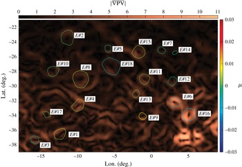
Regions of high PV gradient are also frequently used as indicators of instantaneous ellipticity in unsteady fluid flows. Accordingly, in appendix E, we plot the Elliptic OECSs of figure 3 again over the
 $|\unicode[STIX]{x1D735}$
PV
 $|$
scalar field. Similarly to the OW-criterion, the
 $|\unicode[STIX]{x1D735}$
PV
 $|$
diagnostic highlights regions where no long-lived Lagrangian eddies are present, while it misses regions where such eddies are known to be present.
One may alternatively compute the Lagrangian lifetime of eddies from other objective elliptic LCS detection methods, such as the polar rotation angle (PRA) defined by Farazmand & Haller (Reference Farazmand and Haller2016) or the Lagrangian-averaged vorticity deviation (LAVD) introduced by Haller et al. (Reference Haller, Hadjighasem, Farazmand and Huhn2016). The results (not shown here) obtained in this fashion are close to those in figure 4.
7 Conclusions
We have introduced a frame-invariant, non-dimensional metric to assess the ability of elliptic objective Eulerian coherent structures (OECS) to identify vortical regions with sustained material coherence. Our metric
 $\unicode[STIX]{x1D6E9}_{\unicode[STIX]{x1D6FE}}$
is the ratio between a rotational coherence measure of the vortex and the material leakage out of the vortex.
We have tested the
 $\unicode[STIX]{x1D6E9}_{\unicode[STIX]{x1D6FE}}$
metric on satellite-derived ocean velocity data, where we found that elliptic OECSs with high
 $\unicode[STIX]{x1D6E9}_{\unicode[STIX]{x1D6FE}}$
values tend to forecast the exceptionally coherent Lagrangian vortices found in Haller & Beron-Vera (Reference Haller and Beron-Vera2013) with high probability. To our knowledge, this is the first Eulerian eddy census method that is shown to display a clear correlation with the actual lifetime of nearby Lagrangian vortices. In contrast, we have found other available Eulerian vortex diagnostics to show a distinct lack of correlation with long-term Lagrangian coherence. This is perhaps unsurprising because none of them is non-dimensional or objective, and none of them is inferred from the infinitesimally short-time limit of a mathematically exact Lagrangian coherence criterion. The lack of correlation of classic Eulerian vortex diagnostics with Lagrangian eddy lifetimes is consistent with the findings of Beron-Vera et al. (Reference Beron-Vera, Wang, Olascoaga, Goni and Haller2013) and Wang et al. (Reference Wang, Beron-Vera and Olascoaga2016), who show that these diagnostics overestimate the number of materially coherent vortices significantly.
Our proposed vortex-persistence metric is purely kinematic, and hence offers a model-independent instantaneous forecasting tool. This tool is free from kinetic assumptions, such as conservation or near conservation of vorticity or potential vorticity.
Based on the results presented here, we expect our approach to be useful in real-time transport predictions, environmental decision making and hazard assessment. The purpose of this study has been to demonstrate the predictive power of the proposed persistence metric. A more detailed statistical analysis is planned for future work.
Appendix A. Material flux through elliptic OECSs
Here we derive a formula for the instantaneous material flux through an elliptic OECS
 $\unicode[STIX]{x1D6FE}(t)$
, whose arclength parametrization is denoted by
 $x:s\mapsto x(s)$
, with
 $s\in [0,\unicode[STIX]{x1D70E}]\subset \mathbb{R}$
. The closed curve
 $\unicode[STIX]{x1D6FE}(t)$
is a limit cycle of (3.2), parametrized by
 $s$
, that depends smoothly on the time
 $t$
. We first observe that
 $\unicode[STIX]{x1D6FE}(t+\unicode[STIX]{x1D716}\unicode[STIX]{x0394}t)$
persists for small
 $\unicode[STIX]{x1D716}\unicode[STIX]{x0394}t$
. This is guaranteed by the structural stability of limit cycles of (3.2) together with the smoothness of the underlying flow map. For small enough
 $\unicode[STIX]{x1D716}\unicode[STIX]{x0394}t$
, therefore there exists a nearby elliptic OECS,
 $\unicode[STIX]{x1D6FE}(t+\unicode[STIX]{x1D716}\unicode[STIX]{x0394}t)$
, that is a smooth deformation of
 $\unicode[STIX]{x1D6FE}(t)$
.
Specifically, we can locally represent the perturbed limit cycle as
 $$\begin{eqnarray}\displaystyle x(s,t+\unicode[STIX]{x1D716}\unicode[STIX]{x0394}t) & = & \displaystyle x(s,t)+g(s,t;\unicode[STIX]{x1D716}\unicode[STIX]{x0394}t)\unicode[STIX]{x1D712}^{\bot }(x(s,t),t)\nonumber\\ \displaystyle & = & \displaystyle x(s,t)+\unicode[STIX]{x1D716}\unicode[STIX]{x0394}tg_{1}(s,t)\unicode[STIX]{x1D712}^{\bot }(s,t)+O((\unicode[STIX]{x1D716}\unicode[STIX]{x0394}t)^{2}),\end{eqnarray}$$
where,
 $g$
and
 $g_{1}$
are two smooth scalar functions, and
 $\unicode[STIX]{x1D712}^{\bot }(x(s,t),t)$
is the local normal to the limit cycle at the point
 $x(s,t)\in \unicode[STIX]{x1D6FE}(t)$
. (For notational simplicity we have used
 $\unicode[STIX]{x1D712}$
instead of
 $\unicode[STIX]{x1D712}_{\unicode[STIX]{x1D707}}^{\pm }$
.) The period of the perturbed limit cycle is of the form
 $\unicode[STIX]{x1D70E}_{\unicode[STIX]{x1D716}}=\unicode[STIX]{x1D70E}+\unicode[STIX]{x1D716}\unicode[STIX]{x1D70E}_{1}+O(\unicode[STIX]{x1D716}^{2})$
, leading to the periodicity condition
 $$\begin{eqnarray}x(0,t+\unicode[STIX]{x1D716}\unicode[STIX]{x0394}t)=x(\unicode[STIX]{x1D70E}_{\unicode[STIX]{x1D716}},t+\unicode[STIX]{x1D716}\unicode[STIX]{x0394}t).\end{eqnarray}$$
Taylor expanding this expression with respect to
 $\unicode[STIX]{x1D716}$
and comparing the
 $O(\unicode[STIX]{x1D716})$
terms gives
 $$\begin{eqnarray}{\dot{x}}(\unicode[STIX]{x1D70E},t)={\dot{x}}(0,t)-\unicode[STIX]{x1D712}(x(\unicode[STIX]{x1D70E},t),t){\displaystyle \frac{\unicode[STIX]{x1D70E}_{1}}{\unicode[STIX]{x0394}t}},\end{eqnarray}$$
where the dot denotes the derivative with respect to
 $t$
. This relation shows that the difference between the perturbation to
 $\unicode[STIX]{x1D6FE}(t)$
at
 $s=0$
and at
 $s=\unicode[STIX]{x1D70E}$
, should be in the direction tangential to the limit cycle
 $\unicode[STIX]{x1D6FE}(t)$
in order to ensure its persistence as a
 ${\mathcal{C}}^{1}$
closed curve.
In order to compute the term
 ${\dot{x}}(s,t)$
(in (4.1)), as well as the unknown quantities in (A 3), we write the equation of variations for the ODE (3.2) with respect to changes in the parameter
 $t$
, leading to
 $$\begin{eqnarray}({\dot{x}}(s,t))^{\prime }=\unicode[STIX]{x1D735}\unicode[STIX]{x1D712}(x(s,t),t){\dot{x}}(s,t)+\unicode[STIX]{x2202}_{t}\unicode[STIX]{x1D712}(x(s,t),t),\end{eqnarray}$$
where the prime denotes the derivative with respect to the parameter
 $s$
. Equation (A 4) is a non-autonomous linear ODE for
 ${\dot{x}}(s,t)$
. In the classic theory of dependence of solutions on parameters,
 ${\dot{x}}(0,t)$
is generally zero since initial conditions do not depend on the parameters. In the present case, however, the initial condition,
 $x(0,t)$
does depend on
 $t$
. This dependence determines where the limit cycle is and how it deforms as
 $t$
varies. We rewrite the ODE (A 4) using the following shorthand notation:
 $$\begin{eqnarray}y^{\prime }(s)=A(s)y(s)+c(s),\end{eqnarray}$$
where
 $$\begin{eqnarray}y(s)={\dot{x}}(s,t),\quad A(s)=\unicode[STIX]{x1D735}\unicode[STIX]{x1D712}(x(s,t),t),\quad c(s)=\unicode[STIX]{x2202}_{t}\unicode[STIX]{x1D712}(x(s,t),t),\end{eqnarray}$$
with the time argument
 $t$
suppressed in
 $y,~A$
and
 $c$
for brevity.
Note that
 $y(s)=\unicode[STIX]{x1D712}(x(s,t),t)$
is a solution to the homogeneous part of (A 5). As in Haller & Iacono (Reference Haller and Iacono2003), we solve (A 5) explicitly in the basis
 $[\unicode[STIX]{x1D712}(x(s,t),t),\unicode[STIX]{x1D712}^{\bot }(x(s,t),t)]$
. With the change of coordinates
 $$\begin{eqnarray}y(s)=T(s)z(s),\quad T(s)=[\unicode[STIX]{x1D712}(x(s,t),t),\unicode[STIX]{x1D712}^{\bot }(x(s,t),t)],\end{eqnarray}$$
equation (A 5) can be written as
 $$\begin{eqnarray}z^{\prime }(s)=\tilde{A}(s)z(s)+\tilde{c}(s).\end{eqnarray}$$
Substituting the change of coordinates (A 7) into (A 5) gives
 $$\begin{eqnarray}T^{\prime }(s)z(s)+T(s)z^{\prime }(s)=A(s)T(s)z(s)+c(s).\end{eqnarray}$$
Since
 $T(s)\in \text{SO}(2)$
, equation (A 9) can be written as
 $$\begin{eqnarray}z^{\prime }(s)=[T^{\top }(s)A(s)T(s)-T^{\top }(s)T^{\prime }(s)]z(s)+T^{\top }(s)c(s).\end{eqnarray}$$
Using (A 6)–(A 7), we can write
 $T^{\top }(s)A(s)T(s)$
and
 $T^{\top }(s)T^{\prime }(s)$
as
 $$\begin{eqnarray}\displaystyle & T^{\top }(s)A(s)T(s)=\left[\begin{array}{@{}cc@{}}\langle \unicode[STIX]{x1D712},\unicode[STIX]{x1D735}\unicode[STIX]{x1D712}\unicode[STIX]{x1D712}\rangle & \langle \unicode[STIX]{x1D712},\unicode[STIX]{x1D735}\unicode[STIX]{x1D712}\unicode[STIX]{x1D712}^{\bot }\rangle \\ \langle \unicode[STIX]{x1D712}^{\bot },\unicode[STIX]{x1D735}\unicode[STIX]{x1D712}\unicode[STIX]{x1D712}\rangle & \langle \unicode[STIX]{x1D712}^{\bot },\unicode[STIX]{x1D735}\unicode[STIX]{x1D712}\unicode[STIX]{x1D712}^{\bot }\rangle \end{array}\right], & \displaystyle\end{eqnarray}$$
 $$\begin{eqnarray}\displaystyle & T^{\top }(s)T^{\prime }(s)=\left[\begin{array}{@{}cc@{}}\langle \unicode[STIX]{x1D712},\unicode[STIX]{x1D735}\unicode[STIX]{x1D712}\unicode[STIX]{x1D712}\rangle & \langle \unicode[STIX]{x1D712},R\unicode[STIX]{x1D735}\unicode[STIX]{x1D712}\unicode[STIX]{x1D712}\rangle \\ \langle \unicode[STIX]{x1D712}^{\bot },\unicode[STIX]{x1D735}\unicode[STIX]{x1D712}\unicode[STIX]{x1D712}\rangle & \langle \unicode[STIX]{x1D712}^{\bot },R\unicode[STIX]{x1D735}\unicode[STIX]{x1D712}\unicode[STIX]{x1D712}\rangle \end{array}\right]. & \displaystyle\end{eqnarray}$$
Differentiating the identity
 $\langle \unicode[STIX]{x1D712},\unicode[STIX]{x1D712}\rangle =1$
with respect to
 $x$
, we obtain the following relations
 $$\begin{eqnarray}\left.\begin{array}{@{}c@{}}(\unicode[STIX]{x1D735}\unicode[STIX]{x1D712})^{\top }\unicode[STIX]{x1D712}=0,\quad \langle \unicode[STIX]{x1D712},(\unicode[STIX]{x1D735}\unicode[STIX]{x1D712})^{\top }\unicode[STIX]{x1D712}\rangle =0,\\ \langle \unicode[STIX]{x1D712},\unicode[STIX]{x1D735}\unicode[STIX]{x1D712}\unicode[STIX]{x1D712}\rangle =0,\quad \unicode[STIX]{x1D735}\unicode[STIX]{x1D712}\unicode[STIX]{x1D712}\bot \unicode[STIX]{x1D712},\\ \langle \unicode[STIX]{x1D712}^{\bot },\unicode[STIX]{x1D735}\unicode[STIX]{x1D712}\unicode[STIX]{x1D712}\rangle =\unicode[STIX]{x1D705},\quad R\unicode[STIX]{x1D735}\unicode[STIX]{x1D712}\unicode[STIX]{x1D712}=-\unicode[STIX]{x1D705}\unicode[STIX]{x1D712},\end{array}\right\}\end{eqnarray}$$
where
 $\unicode[STIX]{x1D705}$
denotes the pointwise scalar curvature along the elliptic OECS with respect to the normal vector defined as
 $\unicode[STIX]{x1D712}^{\bot }=R\unicode[STIX]{x1D712}$
. Substituting (A 11)–(A 13) into (A 10) leads to
 $$\begin{eqnarray}\tilde{A}(s)=[T^{\top }(s)A(s)T(s)-T^{\top }(s)T^{\prime }(s)]=\left[\begin{array}{@{}cc@{}}0 & \unicode[STIX]{x1D705}(s)\\ 0 & \langle \unicode[STIX]{x1D712}^{\bot },\unicode[STIX]{x1D735}\unicode[STIX]{x1D712}\unicode[STIX]{x1D712}^{\bot }\rangle \end{array}\right].\end{eqnarray}$$
The invariance property of the trace of a matrix under orthonormal transformations implies that
 $Tr(\unicode[STIX]{x1D735}\unicode[STIX]{x1D712})=Tr(T^{\top }\unicode[STIX]{x1D735}\unicode[STIX]{x1D712}T)$
. Recalling that
 $A=\unicode[STIX]{x1D735}\unicode[STIX]{x1D712}$
, and using (A 11) and (A 13), we obtain
 $$\begin{eqnarray}\displaystyle \unicode[STIX]{x1D735}\boldsymbol{\cdot }\unicode[STIX]{x1D712} & = & \displaystyle Tr(\unicode[STIX]{x1D735}\unicode[STIX]{x1D712})\nonumber\\ \displaystyle & = & \displaystyle Tr(T^{\top }\unicode[STIX]{x1D735}\unicode[STIX]{x1D712}T)\nonumber\\ \displaystyle & = & \displaystyle \langle \unicode[STIX]{x1D712},\unicode[STIX]{x1D735}\unicode[STIX]{x1D712}\unicode[STIX]{x1D712}\rangle +\langle \unicode[STIX]{x1D712}^{\bot },\unicode[STIX]{x1D735}\unicode[STIX]{x1D712}\unicode[STIX]{x1D712}^{\bot }\rangle \nonumber\\ \displaystyle & = & \displaystyle \langle \unicode[STIX]{x1D712}^{\bot },\unicode[STIX]{x1D735}\unicode[STIX]{x1D712}\unicode[STIX]{x1D712}^{\bot }\rangle ,\end{eqnarray}$$
leading to the final form of
 $\tilde{A}(s)$
:
 $$\begin{eqnarray}\tilde{A}(s)=\left[\begin{array}{@{}cc@{}}0 & \unicode[STIX]{x1D705}(x(s,t),t)\\ 0 & \unicode[STIX]{x1D735}\boldsymbol{\cdot }\unicode[STIX]{x1D712}(x(s,t),t)\end{array}\right].\end{eqnarray}$$
Now we derive a simplified expression for the forcing term of the ODE (A 8), i.e. for
 $$\begin{eqnarray}\tilde{c}(s)=T^{\top }(s)c(s)=\left[\begin{array}{@{}c@{}}\langle \unicode[STIX]{x1D712},\unicode[STIX]{x2202}_{t}\unicode[STIX]{x1D712}\rangle \\ \langle \unicode[STIX]{x1D712}^{\bot },\unicode[STIX]{x2202}_{t}\unicode[STIX]{x1D712}\rangle \end{array}\right].\end{eqnarray}$$
To compute
 $\unicode[STIX]{x2202}_{t}\unicode[STIX]{x1D712}$
, we take the partial derivative of the implicit ODE defining elliptic OECSs with respect to
 $t$
to obtain
 $$\begin{eqnarray}\unicode[STIX]{x2202}_{t}\langle \unicode[STIX]{x1D712}(x(s,t),t),[S(r,t)-\unicode[STIX]{x1D707}I]\unicode[STIX]{x1D712}(x(s,t),t)\rangle =0.\end{eqnarray}$$
Dropping the arguments, we find (A 18) equivalent to
 $$\begin{eqnarray}\langle \unicode[STIX]{x1D712},S\unicode[STIX]{x2202}_{t}\unicode[STIX]{x1D712}\rangle =-\frac{\langle \unicode[STIX]{x1D712},\unicode[STIX]{x2202}_{t}S\unicode[STIX]{x1D712}\rangle }{2}.\end{eqnarray}$$
Since the direction field
 $\unicode[STIX]{x1D712}$
is normalized, we have
 $\unicode[STIX]{x2202}_{t}\unicode[STIX]{x1D712}(x,t)\bot ~\unicode[STIX]{x1D712}(x,t)$
, and hence we can write
 $$\begin{eqnarray}\unicode[STIX]{x2202}_{t}\unicode[STIX]{x1D712}(x,t)=\unicode[STIX]{x1D713}(x,t)\unicode[STIX]{x1D712}^{\bot }(x,t),\quad \unicode[STIX]{x1D713}(x,t)\in \mathbb{R}.\end{eqnarray}$$
Substituting (A 20) into (A 19) leads to
 $$\begin{eqnarray}\unicode[STIX]{x1D713}(x(s,t),t)=-\frac{\langle \unicode[STIX]{x1D712},\unicode[STIX]{x2202}_{t}S\unicode[STIX]{x1D712}\rangle }{2\langle \unicode[STIX]{x1D712},S\unicode[STIX]{x1D712}^{\bot }\rangle },\end{eqnarray}$$
which is always defined in the domain
 $U_{\unicode[STIX]{x1D707}}$
, unless
 $\unicode[STIX]{x1D712}\equiv e_{i},i=1,2$
, in which case
 $\langle e_{i},Se_{i}^{\bot }\rangle =0$
.
We are interested in evaluating the instantaneous material flux through elliptic OECSs. Along these curves, the constant instantaneous stretching rate
 $\unicode[STIX]{x1D707}$
is approximately zero, and hence the
 $\unicode[STIX]{x1D712}_{\unicode[STIX]{x1D707}}^{\pm }$
directions are far from the
 $e_{i}$
directions. Specifically, for incompressible flows, the directions
 $\unicode[STIX]{x1D712}_{0}^{\pm }$
exactly bisect the
 $e_{i}$
directions. Therefore, equation (A 21) is always well defined on elliptic OECSs. Substituting (A 20) and (A 21) into (A 17) leads to
 $$\begin{eqnarray}\tilde{c}(s)=\left[\begin{array}{@{}c@{}}0\\ \unicode[STIX]{x1D713}(x(s,t),t)\end{array}\right],\end{eqnarray}$$
as in (4.4).
Using the variation of constants formula (see e.g. Arnold Reference Arnold1973), we can write the solution of (A 8) as
 $$\begin{eqnarray}\displaystyle z(s) & = & \displaystyle \unicode[STIX]{x1D6F7}_{0}^{s}z(0)+\unicode[STIX]{x1D6F7}_{0}^{s}\int _{0}^{s}(\unicode[STIX]{x1D6F7}_{0}^{\unicode[STIX]{x1D717}})^{-1}\tilde{c}(\unicode[STIX]{x1D717})\,\text{d}\unicode[STIX]{x1D717}\nonumber\\ \displaystyle & = & \displaystyle \unicode[STIX]{x1D6F7}_{0}^{s}z(0)+\unicode[STIX]{x1D6F1}(s),\end{eqnarray}$$
with
 $\unicode[STIX]{x1D6F7}_{0}^{s}$
being the normalized fundamental matrix solution to the homogeneous problem
 $$\begin{eqnarray}z^{\prime }(s)=\tilde{A}(s)z(s).\end{eqnarray}$$
By direct integration of (A 24) we obtain
 $$\begin{eqnarray}\unicode[STIX]{x1D6F7}_{0}^{s}=\left[\begin{array}{@{}cc@{}}1 & \displaystyle \int _{0}^{s}\exp \left(\int _{0}^{\unicode[STIX]{x1D717}}\unicode[STIX]{x1D735}\boldsymbol{\cdot }\unicode[STIX]{x1D712}_{\unicode[STIX]{x1D707}}^{\pm }(x(\unicode[STIX]{x1D717},t),t)\,\text{d}\unicode[STIX]{x1D717}\right)\unicode[STIX]{x1D705}(x(\unicode[STIX]{x1D717},t))\,\text{d}\unicode[STIX]{x1D717}\\ 0 & \exp \left(\displaystyle \int _{0}^{s}\unicode[STIX]{x1D735}\boldsymbol{\cdot }\unicode[STIX]{x1D712}_{\unicode[STIX]{x1D707}}^{\pm }(x(\unicode[STIX]{x1D717},t),t)\,\text{d}\unicode[STIX]{x1D717}\right)\end{array}\right],\end{eqnarray}$$
as in (4.3).
Once this fundamental matrix solution is computed, the only missing quantity in (4.2) is the initial condition
 $z(0)$
. To obtain that, we rewrite (A 3) in the
 $z$
coordinates. This, together with (4.2), leads to the system
 $$\begin{eqnarray}\left.\begin{array}{@{}c@{}}z(\unicode[STIX]{x1D70E})=z(0)-d{\displaystyle \frac{\unicode[STIX]{x1D70E}_{1}}{\unicode[STIX]{x0394}t}},\quad d:=[0,1]^{\top }\\ z(\unicode[STIX]{x1D70E})=\unicode[STIX]{x1D6F7}_{0}^{\unicode[STIX]{x1D70E}}z(0)+\unicode[STIX]{x1D6F1}(\unicode[STIX]{x1D70E}).\end{array}\right\}\end{eqnarray}$$
Although this system of equations is undetermined (
 $z(\unicode[STIX]{x1D70E}),z(0)$
and
 $\unicode[STIX]{x1D70E}_{1}$
are unknown), it is sufficient to determine the component of
 $z(0)$
along the
 $\unicode[STIX]{x1D712}^{\bot }$
direction,
 $z^{\bot }(0)$
. Substituting (4.2) and (4.3) into (A 26), we obtain
 $$\begin{eqnarray}\left[\begin{array}{@{}cc@{}}0 & \displaystyle \int _{0}^{\unicode[STIX]{x1D70E}}\exp \left(\int _{0}^{y}\unicode[STIX]{x1D735}\boldsymbol{\cdot }\unicode[STIX]{x1D712}_{\unicode[STIX]{x1D707}}^{\pm }(x(\unicode[STIX]{x1D717},t),t)\,\text{d}\unicode[STIX]{x1D717}\right)\unicode[STIX]{x1D705}(x(y,t))\,\text{d}y\\ 0 & \exp \left(\displaystyle \int _{0}^{\unicode[STIX]{x1D70E}}\unicode[STIX]{x1D735}\boldsymbol{\cdot }\unicode[STIX]{x1D712}_{\unicode[STIX]{x1D707}}^{\pm }(x(\unicode[STIX]{x1D717},t),t)\,\text{d}\unicode[STIX]{x1D717}\right)-1\end{array}\right]\!\!\left[\begin{array}{@{}c@{}}z^{\Vert }(0)\\ z^{\bot }(0)\end{array}\right]=-\!\left[\begin{array}{@{}c@{}}\unicode[STIX]{x1D6F1}^{\Vert }(\unicode[STIX]{x1D70E})\\ \unicode[STIX]{x1D6F1}^{\bot }(\unicode[STIX]{x1D70E})\end{array}\right]-\!\left[\begin{array}{@{}c@{}}1\\ 0\end{array}\right]\!{\displaystyle \frac{\unicode[STIX]{x1D70E}_{1}}{\unicode[STIX]{x0394}t}},\end{eqnarray}$$
where,
 $\exp (\int _{0}^{\unicode[STIX]{x1D70E}}\unicode[STIX]{x1D735}\boldsymbol{\cdot }\unicode[STIX]{x1D712}_{\unicode[STIX]{x1D707}}^{\pm }(x(\unicode[STIX]{x1D717},t),t)\,\text{d}\unicode[STIX]{x1D717})=\unicode[STIX]{x1D70C}_{1}\unicode[STIX]{x1D70C}_{2}=\unicode[STIX]{x1D70C}_{2}$
, with
 $\unicode[STIX]{x1D70C}_{1}$
and
 $\unicode[STIX]{x1D70C}_{2}$
denoting the Floquet multipliers (Guckenheimer & Holmes Reference Guckenheimer and Holmes1983) of the
 $\unicode[STIX]{x1D70E}-$
periodic limit cycle
 $\unicode[STIX]{x1D6FE}$
of the ODE (3.2). Solving this system, we obtain
 $$\begin{eqnarray}\left.\begin{array}{@{}c@{}}z^{\bot }(0)={\displaystyle \frac{\unicode[STIX]{x1D6F1}^{\bot }(\unicode[STIX]{x1D70E})}{1-\unicode[STIX]{x1D70C}_{2}}}\\ \unicode[STIX]{x1D70E}_{1}=\unicode[STIX]{x0394}t\left(\unicode[STIX]{x1D6F1}^{\Vert }(\unicode[STIX]{x1D70E})+z^{\bot }(0)\displaystyle \int _{0}^{\unicode[STIX]{x1D70E}}\exp \left(\int _{0}^{y}\unicode[STIX]{x1D735}\boldsymbol{\cdot }\unicode[STIX]{x1D712}_{\unicode[STIX]{x1D707}}^{\pm }(x(\unicode[STIX]{x1D717},t),t)\,\text{d}\unicode[STIX]{x1D717}\right)\unicode[STIX]{x1D705}(x(y,t))\,\text{d}y\right),\end{array}\right\}\end{eqnarray}$$
where the first equation is the same as (4.5). The equations in (A 28) are independent of the value of
 $z^{\Vert }(0)$
due to the invariance of material flux under a shift of the parameter
 $s$
. The hyperbolic nature of limit cycles ensures that
 $\unicode[STIX]{x1D70C}_{1}\unicode[STIX]{x1D70C}_{2}=\unicode[STIX]{x1D70C}_{2}\neq 1$
, and thus, both expressions in (A 28) are well defined on elliptic OECSs. Observe that the denominator
 $(1-\unicode[STIX]{x1D70C}_{2})$
is equal to the slope of the Poincaré return map along
 $\unicode[STIX]{x1D6FE}$
, as shown in Perko (Reference Perko1990). The first equation of (A 28) is the only component of
 $z(0)$
needed for the computation of the instantaneous material flux
 $\unicode[STIX]{x1D711}_{\unicode[STIX]{x1D6FE}(t)}$
.
Although
 $\unicode[STIX]{x1D70E}_{1}$
is not strictly necessary for computing
 $\unicode[STIX]{x1D711}_{\unicode[STIX]{x1D6FE}(t)}$
, it gives the
 $O(\unicode[STIX]{x1D716})$
variation of the period
 $\unicode[STIX]{x1D70E}_{\unicode[STIX]{x1D716}}$
of to the deformed elliptic OECSs, as the parameter
 $t$
is perturbed to
 $t_{\unicode[STIX]{x1D716}}=t+\unicode[STIX]{x1D716}\unicode[STIX]{x0394}t$
.
Appendix B. Objectivity of the persistence metric
Here we show that the non-dimensional metric
 $\unicode[STIX]{x1D6E9}_{\unicode[STIX]{x1D6FE}}(t)$
is objective i.e. invariant under all coordinate changes of the form
 $$\begin{eqnarray}x=Q(t)\tilde{x}+b(t),\end{eqnarray}$$
where
 $Q(t)\in \text{SO}(2)$
and
 $b(t)\in \mathbb{R}^{2}$
are smooth functions of time. Since the
 $\unicode[STIX]{x1D6E9}_{\unicode[STIX]{x1D6FE}}(t)$
is a scalar quantity, in order for it to be objective (Truesdell & Noll Reference Truesdell and Noll2004), at every point it must have the same value independent of the actual coordinates chosen,
 $x$
or
 $\tilde{x}$
, as long as they are linked by (B 1). To see this, we check objectivity separately for the numerator and denominator of (5.4).
The spin tensor
 $W$
introduced in (2.1) is well known to be non-objective (Truesdell & Noll Reference Truesdell and Noll2004), as it transforms as
 $$\begin{eqnarray}\tilde{W}=Q^{\top }WQ-Q^{\top }\dot{Q}.\end{eqnarray}$$
Correspondingly, the plane-normal component
 $\unicode[STIX]{x1D714}$
of the vorticity transforms under (B 1) as
 $$\begin{eqnarray}\tilde{\unicode[STIX]{x1D714}}=\unicode[STIX]{x1D714}-\unicode[STIX]{x1D714}_{Q},\end{eqnarray}$$
where,
 $\unicode[STIX]{x1D714}_{Q}$
is such that
 $Q^{\top }\dot{Q}=\unicode[STIX]{x1D714}_{Q}R$
. The deviation of the vorticity from its spatial mean transforms as
 $$\begin{eqnarray}\displaystyle \tilde{\unicode[STIX]{x1D714}}-\overline{\tilde{\unicode[STIX]{x1D714}}} & = & \displaystyle \unicode[STIX]{x1D714}-\unicode[STIX]{x1D714}_{Q}-{\displaystyle \frac{1}{A_{\unicode[STIX]{x2202}U}}}\int _{A_{\unicode[STIX]{x2202}U}}(\unicode[STIX]{x1D714}-\unicode[STIX]{x1D714}_{Q})\,\text{d}A\nonumber\\ \displaystyle & = & \displaystyle \unicode[STIX]{x1D714}-{\displaystyle \frac{1}{A_{\unicode[STIX]{x2202}U}}}\int _{A_{\unicode[STIX]{x2202}U}}\unicode[STIX]{x1D714}\,\text{d}A=\unicode[STIX]{x1D714}-\overline{\unicode[STIX]{x1D714}},\end{eqnarray}$$
where, in the second line we used the fact that the domain
 $U$
is time independent and
 $\unicode[STIX]{x1D714}_{Q}$
is space independent. Formula (B 4) proves the objectivity of
 $\unicode[STIX]{x1D714}_{\unicode[STIX]{x1D6FE}(t)}$
defined in (5.1).
To show the objectivity of the relative material leakage defined in (5.3), we rewrite the pointwise material flux density (4.1) in the simplified form:
 $$\begin{eqnarray}\unicode[STIX]{x1D711}=\langle {\dot{x}}_{a1}-{\dot{x}}_{a2},\unicode[STIX]{x0394}x\rangle ,\end{eqnarray}$$
where,
 ${\dot{x}}_{a1}$
and
 ${\dot{x}}_{a2}$
represent two general velocity vectors which have the same base point
 $x_{a}$
, and
 $\unicode[STIX]{x0394}x=x_{a}-x_{b}$
is a simple distance vector between two points. Representing these quantities in the
 $\tilde{x}$
frame, we obtain
 $$\begin{eqnarray}\left.\begin{array}{@{}c@{}}\tilde{{\dot{x}}}_{ai}=Q^{\top }{\dot{x}}_{ai}-Q^{\top }\dot{Q}\tilde{x}_{ai}-Q^{\top }{\dot{b}},\quad i=1,2,\\ \widetilde{\unicode[STIX]{x0394}x}=Q^{\top }\unicode[STIX]{x0394}x,\end{array}\right\}\end{eqnarray}$$
that, together with (B 5) leads to
 $$\begin{eqnarray}\displaystyle \tilde{\unicode[STIX]{x1D711}} & = & \displaystyle \langle -Q^{\top }\dot{Q}(\tilde{x}_{a1}-\tilde{x}_{a2})+Q^{\top }({\dot{x}}_{a1}-{\dot{x}}_{a2}),Q^{\top }\unicode[STIX]{x0394}x\rangle ,\nonumber\\ \displaystyle & = & \displaystyle \langle Q^{\top }({\dot{x}}_{a1}-{\dot{x}}_{a2}),~Q^{\top }\unicode[STIX]{x0394}x\rangle ,\nonumber\\ \displaystyle & = & \displaystyle \unicode[STIX]{x1D711},\end{eqnarray}$$
where, we used the properties of
 $Q$
and that
 $\tilde{x}_{a1}=\tilde{x}_{a2}=\tilde{x}_{a}$
in any coordinate frame since they represent the same base point for the two velocity vectors involved in the material flux computation. We have therefore shown that
 $\unicode[STIX]{x1D714}_{\unicode[STIX]{x1D6FE}}$
and
 $\unicode[STIX]{x1D6E4}_{\unicode[STIX]{x1D6FE}}$
are both objective quantities, and hence so is the vortex-persistence metric,
 $\unicode[STIX]{x1D6E9}_{\unicode[STIX]{x1D6FE}}$
, introduced in Definition 3.
Appendix C. Numerical steps for the computation of elliptic OECSs and
 $\unicode[STIX]{x1D6E9}_{\unicode[STIX]{x1D6FE}}$


Here we propose a systematic way to monitor the accuracy of numerical differentiation involved in (4.3)–(4.4). Specifically, equation (4.3) requires spatial differentiation for the computation of
 $\unicode[STIX]{x1D735}\boldsymbol{\cdot }\unicode[STIX]{x1D712}$
(step (ii)(a)), while (4.4) requires differentiation in time to compute
 $\unicode[STIX]{x2202}_{t}S$
(step (ii)(b)). For the computation of
 $\unicode[STIX]{x2202}_{t}S$
, we employ a backward finite-difference scheme.
To select the appropriate step size for the spatial differentiation of the
 $\unicode[STIX]{x1D712}$
field, we turn the relation
 $(\unicode[STIX]{x1D735}\unicode[STIX]{x1D712})^{\top }\unicode[STIX]{x1D712}=0$
, shown in appendix A, into the scalar equation
 $\langle \unicode[STIX]{x1D712},\unicode[STIX]{x1D735}\unicode[STIX]{x1D712}(\unicode[STIX]{x1D735}\unicode[STIX]{x1D712})^{\top }\unicode[STIX]{x1D712}\rangle =0$
. The deviation of
 $\langle \unicode[STIX]{x1D712},\unicode[STIX]{x1D735}\unicode[STIX]{x1D712}(\unicode[STIX]{x1D735}\unicode[STIX]{x1D712})^{\top }\unicode[STIX]{x1D712}\rangle$
from zero allows to quantitatively monitor the entity of the error due to spatial differentiation in the material flux computation. For instance, a complex geometry of the elliptic OECS would require a finer grid for the accurate computation of
 $\unicode[STIX]{x1D735}\unicode[STIX]{x1D712}$
. This refinement, however, is needed only to handle sharp changes in the elliptic OECSs, which are signalled by high values of the curvature scalar
 $\unicode[STIX]{x1D705}$
. Therefore, it is possible to fix a desired maximum allowable deviation of
 $\langle \unicode[STIX]{x1D712},\unicode[STIX]{x1D735}\unicode[STIX]{x1D712}(\unicode[STIX]{x1D735}\unicode[STIX]{x1D712})^{\top }\unicode[STIX]{x1D712}\rangle$
from zero and select the spatial resolution accordingly.
In a similar fashion, we monitor also the accuracy of numerical finite differencing in the time direction used to compute
 $\unicode[STIX]{x2202}_{t}S$
in (4.4). Since the direction field
 $\unicode[STIX]{x1D712}$
is normalized, differentiating the identity
 $\langle \unicode[STIX]{x1D712}_{\unicode[STIX]{x1D707}},\unicode[STIX]{x1D712}_{\unicode[STIX]{x1D707}}\rangle =1$
with respect to time leads to
 $\unicode[STIX]{x2202}_{t}\unicode[STIX]{x1D712}_{\unicode[STIX]{x1D707}}\bot \unicode[STIX]{x1D712}_{\unicode[STIX]{x1D707}}$
. Monitoring the deviation of
 $|\langle (\unicode[STIX]{x2202}_{t}\unicode[STIX]{x1D712}_{\unicode[STIX]{x1D707}})/(|\unicode[STIX]{x2202}_{t}\unicode[STIX]{x1D712}_{\unicode[STIX]{x1D707}}|),\unicode[STIX]{x1D712}_{\unicode[STIX]{x1D707}}\rangle |$
from zero allows a systematic assessment of the appropriate time step required to compute
 $\unicode[STIX]{x2202}_{t}S$
.
The quantities
 $\langle \unicode[STIX]{x1D712},\unicode[STIX]{x1D735}\unicode[STIX]{x1D712}(\unicode[STIX]{x1D735}\unicode[STIX]{x1D712})^{\top }\unicode[STIX]{x1D712}\rangle$
and
 $|\langle (\unicode[STIX]{x2202}_{t}\unicode[STIX]{x1D712}_{\unicode[STIX]{x1D707}})/(|\unicode[STIX]{x2202}_{t}\unicode[STIX]{x1D712}_{\unicode[STIX]{x1D707}}|),\unicode[STIX]{x1D712}_{\unicode[STIX]{x1D707}}\rangle |$
play the role of numerical reliability parameters and allow us to compute the material flux through any elliptic OECS in an efficient and accurate fashion.
Appendix D. Ocean surface flow dataset
Under the geostrophic assumption, the ocean surface topology measured by satellites plays the role of a streamfunction for the related surface currents. With
 $h$
denoting the sea surface height, the velocity field in longitude–latitude coordinates
 $[\unicode[STIX]{x1D719},~\unicode[STIX]{x1D703}]$
, can be expressed as
 $$\begin{eqnarray}\dot{\unicode[STIX]{x1D719}}=-{\displaystyle \frac{g}{R^{2}f(\unicode[STIX]{x1D703})\cos \unicode[STIX]{x1D703}}}\unicode[STIX]{x2202}_{\unicode[STIX]{x1D703}}h(\unicode[STIX]{x1D719},\unicode[STIX]{x1D703},t),\quad \text{and}\quad \dot{\unicode[STIX]{x1D703}}={\displaystyle \frac{g}{R^{2}f(\unicode[STIX]{x1D703})\cos \unicode[STIX]{x1D703}}}\unicode[STIX]{x2202}_{\unicode[STIX]{x1D719}}h(\unicode[STIX]{x1D719},\unicode[STIX]{x1D703},t),\end{eqnarray}$$
where
 $f(\unicode[STIX]{x1D703}):=2\unicode[STIX]{x1D6FA}\sin \unicode[STIX]{x1D703}$
denotes the Coriolis parameter,
 $g$
the constant of gravity,
 $R$
the mean radius of the earth and
 $\unicode[STIX]{x1D6FA}$
its mean angular velocity. The velocity field is available at weekly intervals, with a spatial longitude–latitude resolution of
 $0.25^{\circ }$
. For more detail on the data, see Beron-Vera et al. (Reference Beron-Vera, Wang, Olascoaga, Goni and Haller2013).
Appendix E. Thresholding requirement for common Eulerian diagnostics
Vortex definitions based on scalar fields (e.g. OW) are often ambiguous due to their dependence on ad hoc thresholding parameters. For the OW-criterion, this threshold value is typically
 $-\unicode[STIX]{x1D6FC}\unicode[STIX]{x1D70E}$
, with
 $\unicode[STIX]{x1D70E}$
being the spatial standard deviation of the OW parameter, and
 $\unicode[STIX]{x1D6FC}\in \mathbb{R}$
selected as a problem-dependent constant. Figure 6 shows the OW level sets for two different values of
 $\unicode[STIX]{x1D6FC}$
: 0.2 and 1, as suggested in Henson & Thomas (Reference Henson and Thomas2008) and Koszalka et al. (Reference Koszalka, Bracco, McWilliams and Provenzale2009), respectively. Note how the values of
 $\unicode[STIX]{x1D6FC}$
can significantly change the overall number and geometry of vortices identified.
Figure 7 shows a total of 61 vortex boundaries (black curves) identified by the OW
 $=-\unicode[STIX]{x1D70E}$
level set (
 $\unicode[STIX]{x1D6FC}=1$
), along with the OW contours. Black numbers denote different vortical regions, while magenta numbers classify their strength in decreasing order of
 $-\overline{\text{OW}}$
.
OW
 $\;(\text{day}^{-1})$
parameter and two specified level sets corresponding to OW
 $=-\unicode[STIX]{x1D70E}$
(black) and OW
 $=-0.2\unicode[STIX]{x1D70E}$
(red) with
 $\unicode[STIX]{x1D70E}$
being the OW spatial standard deviation.

Black contours represent vortex boundaries identified by the Okubo–Weiss level set OW
 $=-\unicode[STIX]{x1D70E}$
, with
 $\unicode[STIX]{x1D70E}$
being the OW spatial standard deviation. Black numbers denote different vortical regions, while magenta numbers classify their strength in decreasing order of
 $-\overline{\text{OW}}$
.

Elliptic OECSs with highest vortex-persistence metric
 $\unicode[STIX]{x1D6E9}_{\unicode[STIX]{x1D6FE}}$
, plotted over
 $|\unicode[STIX]{x1D735}$
PV
 $|\;((\text{deg}\cdot \text{day})^{-1})$
(horizontal colour bar). Elliptic OECSs are encoded with a colour representing their stretching-rate value
 $\unicode[STIX]{x1D707}\;(\text{day}^{-1})$
(right colour bar). Black numbers label different vortical regions encircled by elliptic OECSs.

In figure 8, we show the elliptic OECSs with highest vortex-persistence metric
 $\unicode[STIX]{x1D6E9}_{\unicode[STIX]{x1D6FE}}$
, shown in figure 3, on a scalar field representing the
 $|\unicode[STIX]{x1D735}$
PV
 $|$
where PV is computed with the formula shown in appendix F. Regions of high PV gradient are frequently used indicators of instantaneous ellipticity in unsteady fluid flows. In the south-east of the domain (
 $[1^{\circ }\text{E},7^{\circ }\text{E}]$
,
 $[31^{\circ }\text{S},38^{\circ }\text{S}]$
), although there are several regions of high
 $|\unicode[STIX]{x1D735}$
PV
 $|$
, only one long-lived Lagrangian eddy is present. At the same time,
 $|\unicode[STIX]{x1D735}$
PV
 $|$
fails to signal several other regions captured by elliptic OECSs (see e.g. eddies
 $\#2$
,
 $\#8$
, and
 $\#18$
), where long-lived Lagrangian eddies are present. Therefore, a prediction based only on
 $|\unicode[STIX]{x1D735}$
PV
 $|$
, i.e. choosing an ad hoc threshold parameter to locate vortices instead of using elliptic OECSs, would be even weaker than the one shown in figure 4(c). A similar conclusion holds for the OW-criterion, as discussed in § 6.
Appendix F. Potential vorticity for quasigeostrophic sea surface height flows
In the setting of quasigeostrophic theory in a reduced-gravity shallow-water model, we follow Wunsch (Reference Wunsch1997) and Early et al. (Reference Early, Samelson and Chelton2011) to compute potential vorticity from the sea surface height (SSH)
 $\unicode[STIX]{x1D702}$
as
 $$\begin{eqnarray}\displaystyle \text{PV} & = & \displaystyle \frac{g}{f_{0}}\unicode[STIX]{x0394}\unicode[STIX]{x1D702}+\unicode[STIX]{x1D6FD}_{0}y-\frac{g}{f_{0}L_{D}^{2}}\unicode[STIX]{x1D702}\nonumber\\ \displaystyle & = & \displaystyle \frac{g}{f_{0}}\left(\frac{1}{R^{2}\cos \unicode[STIX]{x1D703}^{2}}\unicode[STIX]{x2202}_{\unicode[STIX]{x1D719}}^{2}+\frac{1}{R^{2}}\unicode[STIX]{x2202}_{\unicode[STIX]{x1D703}}^{2}\right)\unicode[STIX]{x1D702}(\unicode[STIX]{x1D719},\unicode[STIX]{x1D703})+2\unicode[STIX]{x1D6FA}\cos \unicode[STIX]{x1D703}_{0}(\unicode[STIX]{x1D703}-\unicode[STIX]{x1D703}_{0})-\frac{g}{f_{0}L_{D}^{2}}\unicode[STIX]{x1D702}(\unicode[STIX]{x1D719},\unicode[STIX]{x1D703}),\qquad\end{eqnarray}$$
where
 $\unicode[STIX]{x1D703}_{0}$
is the reference latitude for the
 $\unicode[STIX]{x1D6FD}$
-plane;
 $f_{0}=2\unicode[STIX]{x1D6FA}\sin \unicode[STIX]{x1D703}_{0}$
is the constant Coriolis parameter at
 $\unicode[STIX]{x1D703}_{0}$
; and
 $L_{D}$
is the Rossby deformation radius, which can be inferred from Chelton et al. (Reference Chelton, deSzoeke, Schlax, Naggar and Siwertz1998), figure 6, or from http://www-po.coas.oregonstate.edu/research/po/research/rossby_radius. In our analysis, we used
 $\unicode[STIX]{x1D703}_{0}=-30^{\circ }$
which is the mean latitude in the domain, and
 $L_{D}=35~\text{km}$
. We have also observed that the spatial structure of the PV field is insensitive to small changes in
 $L_{D}$
, and small variations in
 $\unicode[STIX]{x1D703}_{0}$
.
The computation of PV from SSH observations alone, is a topic of ongoing research in physical oceanography. Specifically, there is no straightforward way to estimate the stretching component of the PV (see e.g. Lapeyre (Reference Lapeyre2009) for more details).