1. Introduction
Seeds, cysts, and other forms of dormancy generate seed banks, which store genetic information that can be temporarily lost from a population at a certain time and resuscitate later. Having a seed bank is a prevalent evolutionary strategy which has important consequences. For example, in the case of bacteria, it buffers against the selective pressure caused by environmental variability, and at the same time increases genetic variation [Reference González-Casanova10, Reference Lennon and Jones15, Reference Tellier17].
A first attempt to construct a probabilistic model to study this phenomenon was [Reference Kaj, Krone and Lascoux12], which considered a modified Wright–Fisher model in which each individual chooses its parent from the individuals at several generations in the past, and not only from the previous one. This construction has an important technical complication arising from the loss of the Markov property. A new model was defined and studied in [Reference Blath, González-Casanova, Kurt and Wilke-Berenguer1] to avoid this issue. It consists of a two-level discrete Markov chain, which again generalizes the Wright–Fisher model.
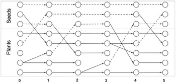
Consider a haploid population of fixed size N which supports a seed bank of constant size M. The N active individuals are called plants, and the M dormant individuals are called seeds. Let
 $0\leq\varepsilon\leq1$
be such that
 $\lfloor\varepsilon N\rfloor\leq M$
. The N plants from generation 0 produce N individuals in generation 1 by multinomial sampling (as in the Wright–Fisher model). However,
 $N-\lfloor\varepsilon N\rfloor$
randomly chosen of these individuals are plants and
 $\lfloor\varepsilon N\rfloor$
are seeds. Then,
 $\lfloor\varepsilon N\rfloor$
uniformly (without replacement) sampled seeds from the seed bank in generation 0 become plants in generation 1. The
 $\lfloor\varepsilon N\rfloor$
seeds produced by the plants in generation 1 take the place of the seeds that germinate. Thus, we again have N plants and M seeds in generation 1 (see Figure 1). This random mechanism is repeated independently to produce the next generations. Observe that this model, unlike [Reference Kaj, Krone and Lascoux12], has non-overlapping reproduction events.
The discrete seed bank model. In this picture
 $N=5$
,
 $M=3$
, and
 $\lfloor\varepsilon N\rfloor = 1$
, i.e. in each generation four plants are produced by active individuals, one seed germinates, and one plant creates one inactive individual.

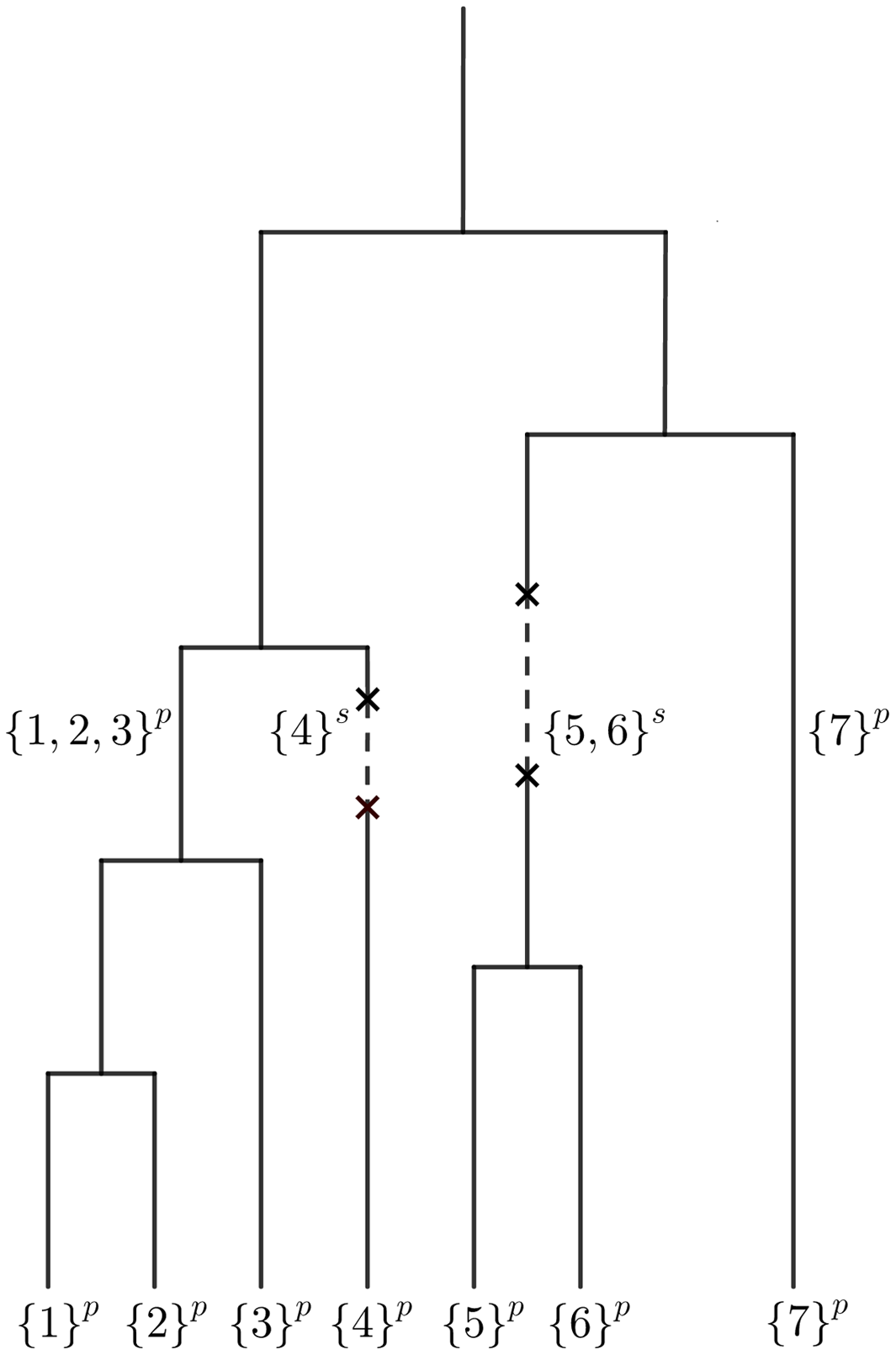
If we let N (and M) go to infinity and rescale the time, the stochastic process that describes the limiting gene genealogy of a sample taken from the seed bank model is called the seed bank coalescent [Reference Blath, González-Casanova, Kurt and Wilke-Berenguer1]. Apart from populations of plants or bacteria, it is remarkable that the seed bank coalescent is a convenient genealogical model for some metapopulations [Reference Lambert and Ma14]. In fact, it was independently introduced in that context and named the peripatric coalescent. It corresponds to a special modification of structured coalescence in which small colonies can emerge from a main population and merge again with it. The seed bank coalescent is a structured coalescent with an active part, having the dynamics of a Kingman coalescent, and a dormant part where the lineages are frozen. Lineages can activate or deactivate at certain rates; see Figure 2 for an illustration.
A possible realization of the seed bank 7-coalescent. Dotted lines indicate inactive individuals and the crosses mean that there is a deactivation or a reactivation.

In this paper we study the asymptotic behavior of some functionals of the seed bank tree that shed light on connections between theoretical and applied population genetics. As an illustration, there is a close relation between the shape of the genealogical tree of a sample of size n and the number of mutations observed in it. More precisely, suppose that mutations appear in the genealogy by simply superimposing a Poisson process on the ancestral lineages (as in the infinite sites model [Reference Durrett7, Section 1.4]). Then, the shape of the tree determines the distribution of the data obtained by DNA sequencing, and it can therefore be inferred from it. For example, conditionally on the total length of the coalescent, denoted by
 $L_n$
, the number of mutations observed in the sample has a Poisson distribution with parameter
 $\mu L_n$
, where
 $\mu$
is the mutation rate. Thus, if we know the asymptotic behavior of the total length of the tree, we can deduce the asymptotic behavior of the number of mutations. This is the key tool for obtaining a Watterson-type estimator for the mutation rate, see [Reference Durrett7]. Not surprisingly, the asymptotics of the total length of many classical coalescents have been studied, e.g. in [Reference Drmota, Iksanov, Möhle and Rösler5, Reference Delmas, Dhersin and Siri-Jégousse2, Reference Kersting13, Reference Diehl and Kersting4].
It was established in [Reference Blath, González-Casanova, Kurt and Wilke-Berenguer1] that the time to the most recent common ancestor of a sample of size n in the seed bank coalescent is of order
 $\log\log n$
. This is an important difference from the classical Kingman coalescent, whose height is finite. Our study establishes that the total length of the tree built from a sample of n plants and zero seeds is of the same order as that of the Kingman coalescent, behaving like
 $\log n$
, but with a different multiplicative constant depending on the activation and deactivation parameters of the model. Moreover, we show that the total active length behaves like the total length of the Kingman coalescent. This means that it is not possible to distinguish between the null Kingman model and the alternative seed bank model using only the tree length (which can be inferred from the number of mutations) unless the dormant individuals have the possibility to mutate while being in the seed bank; that is actually the case in the metapopulation framework described in [Reference Lambert and Ma14]. This conclusion agrees with the main result in [Reference Maughan16], where Maughan observed experimentally that a population of bacteria undergoing dormancy typically does not have a significantly different number of mutations than a population of bacteria not undergoing dormancy. Furthermore, our results offer new insights on the reason for this: most of the mutations occur in the Kingman phase (shortly before the leaves), and in this part of the ancestral tree, dormancy is irrelevant. On the other hand, populations suffering a significant number of mutations while being in the dormant state would be expected to have a higher evolutionary rate. This remark together with [Reference Maughan16] suggests that the mutations that occur to individuals in the latent state are atypical. This is opposed to previous works suggesting that the normal rate of molecular evolution of bacteria with a seed bank is evidence that mutations affecting dormant individuals are frequent [Reference Maughan16].
More theoretical and experimental work is needed to clarify the role of dormancy in the flow of evolution. Finer results, such as sampling formulas, can be derived to discriminate between both null and seed bank models. For the time being, we are able to describe the seed bank tree in detail as it undergoes different phases. It can be said that we describe the shape of the seed bank tree.
1.1. Main results
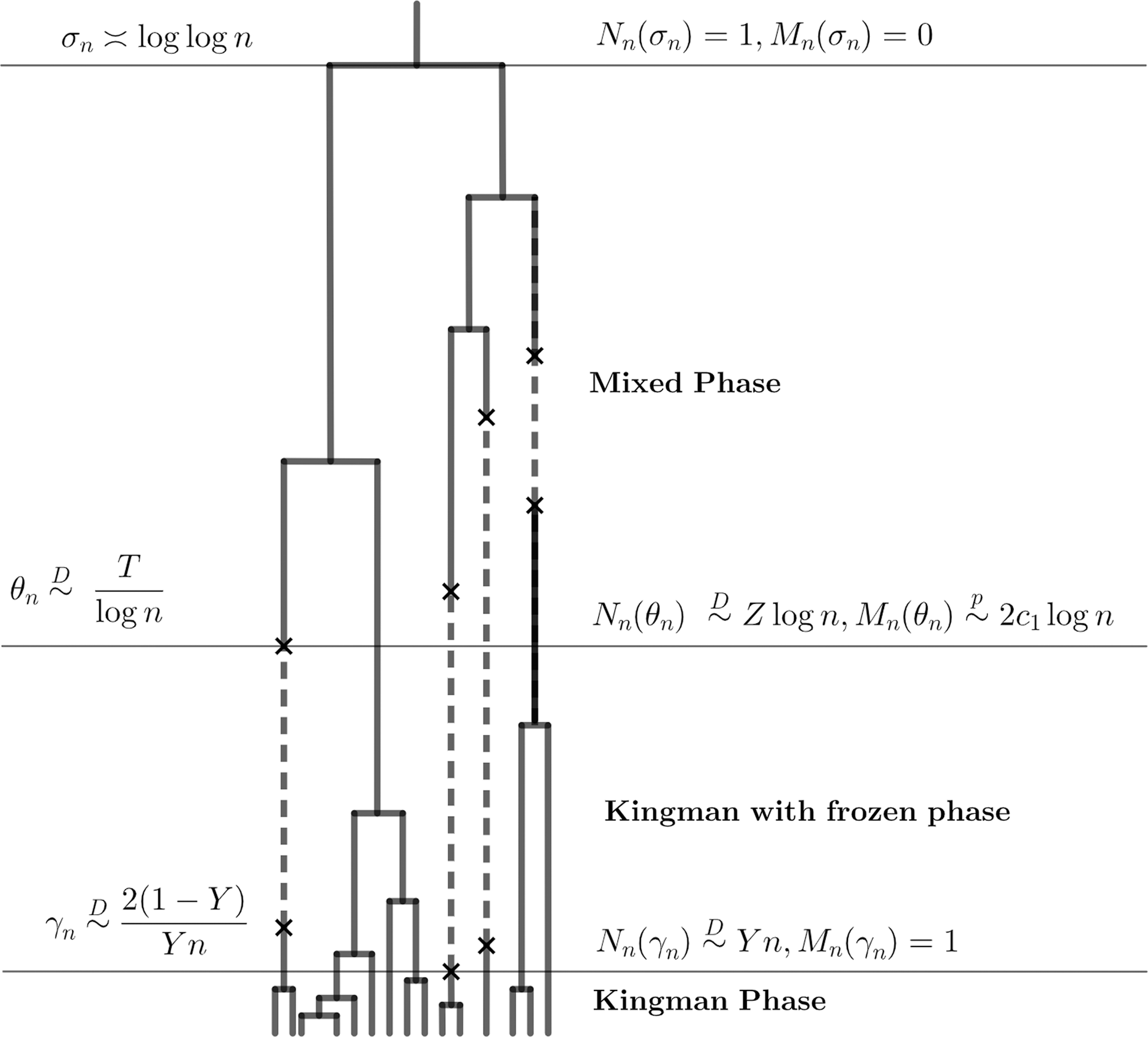
We study some relevant stopping times of the seed bank coalescent, leading to a complete description of the shape of the tree and explaining how long the genealogies spend in successive dynamical phases, as detailed precisely in Table 1 and Figure 3.
Summary of the asymptotic behavior of the functionals of the seed bank coalescent studied in this work. Here, Y is a
 $\text{Beta}(2c_1,1)$
distributed random variable, T is an exponential random variable with parameter
 $2c_1c_2$
, and Z is a Fréchet random variable with shape parameter 1 and scale parameter
 $4c_1c_2$
.

Summary of the asymptotic behavior of the functionals of the seed bank coalescent studied in this work. Here, Y is a
 $\text{Beta}(2c_1,1)$
distributed random variable, T is an exponential random variable with parameter
 $2c_1c_2$
, and Z is a Fréchet random variable with shape parameter 1 and scale parameter
 $4c_1c_2$
. The symbol
 $A_n\overset{\text{p}}\sim B_n$
means that
 $\frac{A_n}{B_n}\to1$
in probability. The symbol
 $A_n\overset{\mathcal D}\sim XB_n$
means that
 $\frac{A_n}{B_n}\to X$
in distribution. The symbol
 $A_n\asymp B_n$
means that
 $C_1B_n\leq\mathbb{E}[{A_n}]\leq C_2{B_n}$
for some constants
 $C_1,C_2$
.

Let us now define the seed bank coalescent properly. Fix
 $n\in\mathbb N$
and let
 $\mathcal{P}_n$
be the set of partitions of
 $[n]\,:\!=\,\lbrace 1,2, \ldots ,n\rbrace $
. Then the set of marked partitions
 $\mathcal{P}_n^{\lbrace \text{p},\text{s} \rbrace }$
is constructed from
 $\mathcal{P}_n$
by adding a flag (either p for a plant or s for a seed) to each block of the partition. For example, for
 $n=7$
,
 $\pi=\lbrace \lbrace 1,2 ,3\rbrace ^{\text{p}},\lbrace 4\rbrace ^{\text{s}},\lbrace 5,6\rbrace ^{\text{s}},\lbrace 7 \rbrace ^{\text{p}}\rbrace $
is an element of
 $\mathcal{P}_7^{\lbrace \text{p},\text{s} \rbrace }$
. The seed bank n-coalescent
 $(\Pi_{n}(t))_{t\geq0}$
, with deactivation intensity
 $c_1>0$
and activation intensity
 $c_2>0$
, is the continuous-time Markov chain with values in
 $\mathcal{P}_n^{\lbrace \text{p},\text{s} \rbrace }$
having the following dynamics. As for the Kingman coalescent, each pair of plant blocks merges at rate 1, independent of each other. Moreover, any block can change its flag from p to s at rate
 $c_1$
, and vice versa at rate
 $c_2$
; see Figure 2 for an illustration.
The block-counting process of the seed bank n-coalescent is the two-dimensional Markov chain
 $\big(N_n(t),M_n(t)\big)_{t\geq0}$
with values in
 $([n]\cup\{0\})\times([n]\cup\{0\})$
and the following transition rates, for
 $t\geq0$
:
 \begin{equation*} \big(N_n(t),M_n(t)\big)\text{ jumps from }(i,j)\text{ to}\!\left\{ \begin{array}{l@{\quad}l@{\quad}l}(i-1,j) & \textrm{ at rate } \binom{i}{2} & \mbox{(coalescence)},\\[4pt](i-1,j+1) & \textrm{ at rate } c_1i &\mbox{(deactivation)},\\[4pt](i+1,j-1) & \textrm{ at rate } c_2j &\mbox{(activation)}.\end{array}\right .\end{equation*}
Note that
 $N_n(t)$
can have either an upward jump if a seed becomes a plant, or a downward jump if there is a coalescence event or a plant becomes a seed. Also observe that each jump has size one. In the following, we suppose that
 $N_n(0)=n$
and
 $M_n(0)=0$
.
For
 $i\in[n]$
, we denote by
 $\tau_n^i$
the hitting time of level i by the process
 $N_n$
, i.e.
 ${\tau}_n^n=0$
and
 \begin{equation} \tau_n^i=\inf\{t\geq0 \,:\, N_n(t)=i\}.\end{equation}
Furthermore, let
 $\gamma_n$
and
 $\theta_n$
be, respectively, the first time that some plant becomes a seed and the first time that some seed becomes a plant, i.e.
 \begin{align} \gamma_n & = \mbox{inf}\lbrace t>0 \,:\, M_n({t-})<M_n(t)\rbrace =\mbox{inf}\lbrace t>0 \,:\, M_n(t)=1\rbrace , \end{align}
 \begin{align} \theta_n & =\inf\{t>0 \,:\, M_n(t{-})>M_n(t)\}. \end{align}
Finally, denote by
 $\sigma_n$
the time to the most recent common ancestor, already studied in [Reference Blath, González-Casanova, Kurt and Wilke-Berenguer1],
 $\sigma_n=\mbox{inf}\lbrace t>0 \,:\, N_n(t)+M_n(t)=1\rbrace =\mbox{inf}\lbrace t>0 \,:\, N_n(t)=1,M_n(t)=0\rbrace $
.
We first obtain asymptotic results on the random variables
 $\gamma_n$
and
 $\theta_n$
and the size of the system at those times. The results obtained in Sections 2 and 3 are summarized in Table 1 and Figure 3.
Observe that the rate of coalescence is quadratic with respect to the number of plants, while the rate of deactivation (resp. the rate of activation) is linear with respect to the number of plants (resp. the number of seeds). From [Reference Blath, González-Casanova, Kurt and Wilke-Berenguer1], we inferred that the number of seeds accumulated until time
 $\theta_n$
,
 $M_n(\theta_n)$
, is of order
 $\log n$
. Lemma 3.3 suggests that, until time
 $\tau_n^{\lfloor (\!\log n)^a\rfloor}$
, for
 $a>1/2$
, the block-counting process
 $(N_n(t))_{t\ge0}$
behaves similarly to that of the Kingman coalescent. However, at time
 $\tau_n^{\lfloor \sqrt{\log n}\rfloor}$
, the system reaches a level of
 $\sqrt{\log n}$
plants and the times of decay are no longer close to those of the Kingman coalescent. Indeed, at this time, we argue that the number of seeds is still of order
 $\log n$
and the coalescence events no longer dominate the dynamics. The seed bank coalescent then enters a mixed regime with coalescence and activation occurring at the same velocity.
In Section 4 we analyze the total length
 \begin{equation} L_n=A_n+I_n ,\end{equation}
where the active and inactive lengths are defined by
 \begin{equation} A_n=\int_0^{\sigma_n}N_n(t) \, \text{d} t , \qquad I_n=\int_0^{\sigma_n}M_n(t) \, \text{d} t.\end{equation}
Our main result is stated as follows.
Theorem 1.1. Consider the seed bank coalescent starting with n plants and no seeds. Then,
 \begin{equation*}\lim_{n\rightarrow\infty}\frac{L_n}{\log n}=2\!\left(1+\frac{c_1}{c_2}\right) \quad {in\ probability.}\end{equation*}
Interestingly, the numerical techniques of [Reference Hobolth, Siri-Jégousse and Bladt11] used to study the total length for fixed n show that the balance between active and inactive lengths is equally conserved for their expectations for any
 $n\geq2$
,
 ${c_1}\mathbb{E}[A_n]=c_2\mathbb{E}[I_n]$
. The behavior of both
 $A_n$
and
 $I_n$
is obtained by considering those variables before and after the time of the first activation
 $\theta_n$
. Hence, the results of Section 3 are key tools for the forthcoming proofs. Theorem 1.1 also gives an immediate corollary on the number of active and inactive mutations on the seed bank tree.
Corollary 1.1. Consider the seed bank coalescent starting with n plants and no seeds. Let
 $S_n$
be the number of mutations in the seed bank tree. Let
 $\mu$
be the mutation rate for the active individuals and let
 $\kappa$
be the mutation rate for the inactive individuals. Then
 \begin{equation*}\lim_{n\rightarrow\infty}\frac{S_n}{\log n}=2\!\left(\mu+\kappa\frac{c_1}{c_2}\right) \quad {in\ probability.}\end{equation*}
Finally, in Section 5 we establish a sampling formula inspired by Watterson’s ideas in [Reference Watterson18], which helps us to understand the fine configuration of the blocks of a seed bank coalescent at given times.
2. The time of the first deactivation
We start with the study of
 $\gamma_n$
, the time of the first deactivation defined in (1.2), and the size of the system at this time. Observe that if
 $N_n(0)=n$
and
 $M_n(0)=0$
, there are
 $n-N_n(\gamma_n){-1}$
coalescence events until time
 $\gamma_n$
and we can write
 $\gamma_n=\sum_{i=N_n(\gamma_n)+1}^{n}V_i$
, where the
 $V_i$
are independent exponential random variables with respective parameters
 $\binom{i}{2}+c_1i$
.
We start with an easy limit result on the variable
 $N_n(\gamma_n)$
. Note that, in a classical Kingman coalescent with mutations appearing at rate
 $c_1$
, the quantity
 $n-N_n(\gamma_n){-1}$
can also be interpreted as the number of coalescence events before the most recent mutation in the genealogy. Recent studies on the shape of coalescent trees at the time of the first mutation in a branch can be found in [Reference Freund and Siri-Jégousse8], with some direct applications to coalescent model selection [Reference Freund and Siri-Jégousse9].
Proposition 2.1. Consider a seed bank coalescent starting with n plants and no seeds. Then
 $\lim_{n\rightarrow\infty}\{N_n(\gamma_n) / n\} = Y$
in distribution, where
 $Y\sim \text{Beta}(2c_1,1)$
.
Proof.Let
 $z\in(0,1)$
. We have
 \begin{equation*}\mathbb{P}(N_n(\gamma_n)\leq zn) = \prod_{i=\lfloor zn\rfloor+1}^{n}\frac{\binom{i}{2}}{\binom{i}{2}+c_1i}= \prod_{i=\lfloor zn\rfloor}^{n-1}\dfrac{i}{i+2c_1} = \exp \!\left\lbrace - \!\! \sum_{i=\lfloor zn\rfloor}^{n-1} \!\! \log\!\left( 1+\dfrac{2c_1}{i}\right)\right\rbrace .\end{equation*}
Using that
 $\log(1+x)\sim x$
near 0, we obtain
 \begin{equation*}\mathbb{P}(N_n(\gamma_n)\leq zn) \sim \exp \!\left\lbrace -\sum_{i=\lfloor zn\rfloor}^{n-1}\frac{2c_1}{i}\right\rbrace \sim \exp \!\left\lbrace {-2c_1}\log\!\left(\frac{1}{z}\right)\right\rbrace = z^{2c_1} ,\end{equation*}
which is the distribution function of a Beta
 $(2c_1,1)$
random variable.
We now establish the asymptotic behavior of the time of the first deactivation,
 $\gamma_n$
.
Proposition 2.2. Consider a seed bank coalescent starting with n plants and no seeds. Then,
 \begin{equation} \lim_{n\rightarrow\infty}n\gamma_n=\Gamma\,:\!=\,\dfrac{2(1-Y)}{Y} \end{equation}
in distribution, where Y is Beta
 $(2c_1,1)$
distributed. The density function of
 $\Gamma$
is
 \begin{equation*}f_\Gamma(x)=c_1\!\left(\dfrac{2}{2+x}\right)^{2c_1+1}\end{equation*}
for
 $x\geq0$
. In particular, if
 $c_1>{1}/{2}$
, then the expectation of
 $\Gamma$
is finite,
 \begin{equation*}\mathbb{E}[\Gamma]=\frac{2}{2c_1-1}, \end{equation*}
and if
 $c_1>1$
, the variance of
 $\Gamma$
is finite,
 \begin{equation*} \text{Var}(\Gamma)=\frac{4c_1}{(c_1-1)(2c_1-1)^2}. \end{equation*}
Proof.Let
 $G_n(0)=0$
and, for
 $t\in (0,1)$
, define
 \begin{equation*} G_n({t})=\sum_{i=\lfloor (1-t)n \rfloor+1}^nV_i=\sum_{i=\lfloor (1-t)n \rfloor+1}^n\dfrac{2e_i}{i(i-1+2c_1)}, \end{equation*}
where the
 $e_i$
are independent and identically distributed (i.i.d.) standard exponential random variables. With this notation, we obtain
 $\gamma_n=G_n\!\left(1-N_n(\gamma_n)/n\right)$
.
We first show that, for any
 $t\in (0,1)$
, we have
 \begin{equation} \lim_{n\rightarrow\infty}\!\left( nG_n(s)\right)_{s\leq t}= \left( \dfrac{2s}{1-s}\right)_{s\leq t}\end{equation}
in distribution, in the sense of weak convergence in the path space D[0, t]. To this end, we first establish that, for a fixed
 $t\in(0,1)$
,
 \begin{equation} \lim_{n\rightarrow\infty}nG_{n}(t)= \dfrac{2t}{1-t}\end{equation}
in
 $L^2$
. By definition, we have that
 \begin{equation*}\mathbb{E}[nG_n(t)]= \sum_{i=\lfloor (1-t)n \rfloor+1}^{n}\frac{2n}{i(i-1+2c_1)} \sim \frac{1}{n}\sum_{i=\lfloor (1-t)n \rfloor+1}^{n}\frac{2}{(i/n)^2}.\end{equation*}
By a Riemann sum argument, we obtain
 \begin{equation*}\mathbb{E}[nG_n(t)]\sim\int_{1-t}^1 \dfrac{2}{x^{2}} \, \text{d} x = \dfrac{2t}{1-t}.\end{equation*}
Now, by the independence of the random variables
 $e_i$
,
 \begin{equation*}\text{Var}(nG_n(t))= \sum_{i=\lfloor (1-t)n \rfloor+1}^{n}\frac{4n^2}{i^2(i-1+2c_1)^2} \sim \sum_{i=\lfloor (1-t)n \rfloor+1}^{n}\frac{4n^2}{i^4}.\end{equation*}
Again, by a Riemann sum argument we obtain that
 $\text{Var}(nG_n(t))$
converges to 0 as
 $n\to\infty$
. This gives (2.3).
To obtain (2.2) we follow the same steps as [Reference Dhersin, Freund, Siri-Jégousse and Yuan3, Proposition 6.1], with
 $\alpha=2$
. Then, the proof of (2.1) follows by adapting the alternative proof of [Reference Dhersin, Freund, Siri-Jégousse and Yuan3, Theorem 5.2, p. 1713], taking
 $\alpha=2$
and the limit variable
 $\sigma$
being
 $1-Y$
and Beta
 $(1, 2c_1)$
distributed.
The distribution function of
 $\Gamma$
is given by
 \begin{equation*}\mathbb{P}\!\left( \Gamma\leq x\right) = \mathbb{P}\!\left( Y\geq \frac{2}{2+x}\right) = 1-\left(\frac{2}{2+x} \right)^{2c_1}, \quad x\geq0 .\end{equation*}
We get the density by differentiating. The moments of
 $\Gamma$
are obtained by computing
 \begin{equation*}\mathbb{E}\big[\Gamma^k\big]=\int_0^\infty kx^{k-1}\mathbb{P}(\Gamma>x) \, \text{d} x = \int_0^\infty kx^{k-1}\!\left(\frac{2}{2+x} \right)^{2c_1} \text{d} x.\end{equation*}
In particular, the kth moment is finite for
 $c_1>k/2$
.
3. The time of the first activation
In this section we study
 $\theta_n$
, the first time that a seed becomes a plant, which we introduced in (1.3). We also provide some limit laws for
 $N_n({\theta_n})$
and
 $M_n({\theta_n})$
. Observe that from time zero up to time
 $\theta_n$
only two types of event occur, either coalescence or deactivation. Recall the successive hitting times of the chain
 $N_n$
, denoted by
 $\big(\tau_{n}^i\big)_{i=1}^n$
and defined in (1.1).
Proposition 3.1. Consider a seed bank coalescent starting with n plants and no seeds. Then the following asymptotics hold:
 \begin{equation} \lim_{n\rightarrow\infty} \frac{N_{n}({\theta_n})}{\log n}=Z \quad {in\ distribution,}\end{equation}
where Z is a Fréchet random variable with shape parameter 1 and scale parameter
 $4c_1c_2$
, with distribution function
 $\mathbb{P}(Z\leq z)=\exp\{-4c_1c_2/z\}$
. Also,
 \begin{equation} \lim_{n\rightarrow\infty} \frac{M_{n}({\theta_n})}{\log n}=2c_1 \quad {in\ probability.}\end{equation}
Finally,
 \begin{equation}\lim_{n\rightarrow\infty} {\log n\theta_n}=T \quad {in\ distribution,}\end{equation}
where T is an exponential random variable with parameter
 $2c_1c_2$
.
The proof of (3.2) is obtained by combining Lemmas 3.1 and 3.4 The proof of (3.1) and (3.3) is obtained by combining Lemmas 3.2 and 3.5, which appear in the following. We get these results by coupling the seed bank coalescent with two simpler models.
The colored seed bank coalescent (see [Reference Blath, González-Casanova, Kurt and Wilke-Berenguer1, Definition 4.2]) is a marked coalescent where each element of [n] additionally has a flag indicating its color: white or blue. Movements and mergers of the blocks of the colored coalescent follow the same dynamics as those of the classical seed bank coalescent. Additionally, if a block activates, each individual inside this block gets the color blue. In other cases the colors remain unchanged.
As in [Reference Blath, González-Casanova, Kurt and Wilke-Berenguer1], we start with all individuals colored white, so blue only appears after a reactivation event, and we also use the notation
 $\underline{\text{N}}_{n}(t)$
(resp.
 $\underline{\text{M}}_{n}(t)$
) for the number of white plants (resp. white seeds) at time t, starting with n (white) plants and zero seeds.
The notation for the reaching times of
 $\underline{\text{N}}_{n}$
are
 $\underline{\tau}_n^n=0$
and, for
 $i\in[n-1]$
,
 $\underline{\tau}_n^i=\inf\lbrace t>0 \,:\, \underline{\text{N}}_n({t})=i\rbrace $
.
Note that, on the event
 $\big\{\tau_n^i<\theta_n\big\}$
, we have
 $\underline \tau_n^i=\tau_n^i$
almost surely (a.s.), and in general the following stochastic bound holds:
 \begin{equation} \underline{\tau}_n^{i-1}-\underline{\tau}_n^{i}\leq_{st}\tau_n^{i-1}-\tau_n^{i} .\end{equation}
This model is of particular use to prove that the number of seeds that “survive” up to moment
 $\theta_n$
is of order
 $\log n$
. More precisely, as in [Reference Blath, González-Casanova, Kurt and Wilke-Berenguer1], consider the independent Bernoulli random variables
 $B^i_{n}= \textbf{1}_{\lbrace \text{deactivation\ at\ }\underline{\tau}_n^i\rbrace }$
for
 $i\in[n-1]$
, with respective parameter
 \begin{equation}\mathbb{P}\big(B^i_{n}=1\big) = \frac{c_1(i+1)}{\binom{i+1}{2}+c_1(i+1)} = \dfrac{2c_1}{i+2c_1},\end{equation}
independently of the number of seeds in the system. It is clear that, almost surely for any
 $t\geq0$
,
 $M_n(t)\leq\sum_{i=1}^{n-1}B_n^i$
. This and Bienaymé–Chebyshev’s inequality lead to the following straightforward result.
Lemma 3.1. For any
 $\varepsilon>0$
,
 \begin{equation} \mathbb{P}\bigg(\!\sup_{t\geq0} M_{n}({t})>2c_1(1+\varepsilon)\log n\bigg)\leq\frac{1}{2c_1\varepsilon^2\log n}. \end{equation}
In particular, for any
 $\varepsilon>0$
,
 $\lim_{n\rightarrow\infty}\mathbb{P}\big( M_{n}({\theta_n})\leq2c_1(1+\varepsilon)\log n\big)=1$
.
From now on, denote the upper bound
 $m_n \,:\!=\,\lfloor2c_1(1+\varepsilon)\log n\rfloor$
for
 $\varepsilon>0$
. We will use this notation in the following proofs.
The bounded seed bank coalescent is a modification of the original seed bank coalescent, where only m seeds can be accumulated in the bank. Thus, when the bank is full, a deactivating lineage disappears instead of moving to the bank. In our case, we start with n plants and m seeds (the bank is full from the beginning).
Denote by
 $\bar{N}_{n,m}(t)$
(resp.
 $\bar{M}_{n,m}(t)$
) the number of plants (resp. seeds) at time t in the bounded coalescent starting with n plants and m seeds. The block-counting process of the bounded coalescent with parameters
 $c_1,c_2>0$
has the following transition rates for
 $ i\leq n$
and
 $j\leq m$
:
 \begin{equation*}\big(\bar{N}_{n,m}(t),\bar{M}_{n,m}(t)\big)\text{ jumps from }(i,j)\text{ to}\!\left\{ \begin{array}{l@{\quad}l@{\quad}l}(i-1,j) & \textrm{at rate } \binom{i}{2}+c_1i{\bf 1}_{\{j= m\}},\\[3pt](i-1,j+1) & \textrm{at rate } c_1i{\bf 1}_{\{j<m\}},\\[3pt](i+1,j-1) & \textrm{at rate } c_2j.\\\end{array}\right .\end{equation*}
By coupling the seed bank coalescent with its bounded version, we obtain a lower bound for
 $\theta_n$
and an upper bound for
 $N_n(\theta_n)$
.
Lemma 3.2. Recall T and Z from Proposition 3.1. We have
 \begin{align} \lim_{n\rightarrow\infty}\mathbb{P}\big( {\theta_n}\log n\leq t\big) & \leq \mathbb{P}(T\leq t) , \end{align}
 \begin{align} \lim_{n\rightarrow\infty} \mathbb{P}\big( {N_n({\theta_n}})>z{\log n}\big) & \leq \mathbb{P}\!\left( Z>z\right). \end{align}
Proof.On the event
 $\big\{M_{n}({\theta_n})\leq m_n\big\}$
, which occurs asymptotically with probability 1 by Lemma 3.1, the variable
 $\theta_n$
is bounded from below, stochastically, by the random variable
 $\bar\theta_{n,m_n}$
defined by
 $\bar\theta_{n,m_n}=\inf\big\{t\geq0 \,:\, \bar M_{n,m_n}(t{-})>\bar M_{n,m_n}(t) \big\}$
and having exponential distribution with parameter
 $c_2m_n$
. Then, for
 $t>0$
,
 \begin{align*} \mathbb{P}\big(\theta_n\log n\leq{t} \big) & = \mathbb{P} \big(\theta_n\log n\leq{t}, M_{n}({\theta_n})\leq m_n \big)+o(1) \\ & \leq \mathbb{P} \!\left(\bar\theta_{n,m_n}\log n\leq{t}\right)+o(1) \\ & = 1-\exp\!\left\{-t\frac{c_2\lfloor2c_1(1+\varepsilon)\log n\rfloor}{\log n}\right\}+o(1).\end{align*}
So, for any
 $\varepsilon>0$
,
 $\lim_{n\rightarrow\infty}\mathbb{P}\big(\theta_n\log n\leq{t} \big)\leq\mathbb{P}\!\left(T\leq t(1+\varepsilon)\right)$
. This gives (3.7).
To prove (3.8), observe that, on the event
 $\big\{M_{n}({\theta_n})\leq m_n\big\}$
, the variable
 $N_n(\theta_n)$
is bounded from above, stochastically, by the random variable
 $\bar N_{n,m_n}\big(\bar\theta_{n,m_n}\big)$
. So,
 \begin{equation} \mathbb{P}\big( {N_n({\theta_n}})>z{\log n}\big)\leq\mathbb{P}\big( {\bar N_{n,m_n}\big({\bar\theta_{n,m_n}}\big)}>z{\log n}\big)+\mathbb{P}\big(M_{n}({\theta_n})> m_n\big).\end{equation}
Let us study the asymptotic of
 $\bar N_{n,m_n}\big(\bar\theta_{n,m_n}\big)$
. With similar arguments to Proposition 2.1, we have
 \begin{align*} \mathbb{P}\big(\bar N_{n,m_n}\big(\bar\theta_{n,m_n}\big)\leq z\log n\big) & = \prod_{i=\lfloor z\log n\rfloor+1}^n\frac{\binom{i}{2}+c_1i}{\binom{i}{2}+c_1i+c_2m_n} \\ & = \exp\!\left\{ -\sum_{i=\lfloor z\log n\rfloor+1}^n\log\!\left( 1+\frac{2c_2m_n}{i(i-1+2c_1)}\right) \right\} \\ & \sim \exp\!\left\{ -2c_2m_n\sum_{i=\lfloor z\log n\rfloor+1}^n\frac{1}{i^2}\right\}.\end{align*}
By a Riemann sum argument, we know that
 \begin{equation} \lim_{n\rightarrow\infty}m_n\sum_{i=\lfloor z\log n\rfloor+1}^n\frac{1}{i^2}=2c_1(1+\varepsilon)\int_z^\infty\frac{1}{x^2} \, \text{d} x = \frac{2c_1(1+\varepsilon)}{z}.\end{equation}
Since
 $\mathbb{P}(Z\leq z)=\exp\{-{4c_1c_2}/{z}\}$
, we obtain, by taking the limits in (3.9), that
 $\lim_{n\rightarrow\infty} \mathbb{P}\big( {N_n({\theta_n}})>z{\log n}\big)\leq\mathbb{P}\!\left( Z>z/(1+\varepsilon)\right)$
, which implies (3.8).
The bounded seed bank coalescent is also useful to bound from above the random variable
 $N_n(t)$
, for any
 $t\geq0$
. Let
 $(K_n(t))_{t\geq0}$
stand for the block-counting process of the Kingman coalescent starting with n lineages. Let
 $(\chi_i(t))_{i\geq 1}$
be a sequence of i.i.d. Bernoulli variables of parameter
 $1-\exp\!({-}c_2t)$
. Those variables are more easily understood as
 $\chi_i(t)={\bf 1}_{\{{e}_i<c_2t\}}$
, where the
 ${e}_i$
are i.i.d. standard exponential variables. It is easy to see that, on the event
 $\big\{\!\sup_{t\geq 0} M_n(t)\leq m\big\}$
, stochastically,
 \begin{equation} N_n(t)\leq K_n(t)+\sum_{i=1}^{m}\chi_i(t).\end{equation}
This follows because
 $K_n(t)$
bounds the number of blocks that have not been deactivated before time t, and
 $\sum_{i=1}^{m}\chi_i(t)$
bounds the number of blocks that have already reactivated. Both processes are independent.
We now prove a useful lemma thanks to the two couplings introduced previously. To simplify the notations here and in the followibg, denote
 $\tau_n^{\lfloor (\!\log n)^a\rfloor}$
by
 $\tau_n^{(a)}$
, for any
 $a>0$
.
Lemma 3.3. For
 $a>b\geq0$
such that
 $a+b>1$
,
 $\lim_{n\rightarrow\infty} \mathbb P\Big(\tau_n^{(a)}\leq{(\!\log n)^{-b}}\Big)=1$
.
Proof.Within this proof we denote
 $m_n:=\lceil 2c_1(1+\varepsilon)\log n\rceil$
. Let
 $E_n=\big\{\!\sup_tM_n({t})\leq m_n\big\}$
. We start by observing that
 $\mathbb P\Big(\tau_n^{(a)}>{(\!\log n)^{-b}}\Big)=\mathbb P\Big(\tau_n^{(a)}>{(\!\log n)^{-b}}, E_n\Big)+\mathbb P\Big(\tau_n^{(a)}>{(\!\log n)^{-b}}, E_n^{\text{c}}\Big)$
. From (3.6), we get
 \begin{equation*}\mathbb P\big( E_n^{\text{c}}\big)\leq\frac{1}{2c_1\varepsilon^2\log n} , \end{equation*}
so it just remains to control the probability on the event
 $E_n$
. Recall
 $(K_n(t))_{t\geq0}$
and
 $(\chi_i(t))_{i\geq 1}$
from (3.11). Let
 $\omega_{n,a}=\inf\big\{t>0 \,:\, K_n(t)=\big\lfloor\frac{1}{2}(\!\log n)^{a}\big\rfloor\big\}$
. Observe that
 \begin{align*} \big\{\tau_n^{(a)}>t,E_n\big\} & = \big\{N_n(t)>(\!\log n)^{a},E_n\big\} \\ & \subset \Bigg\{K_n(t)+\sum_{i=1}^{m_n} \chi_i(t)>(\!\log n)^{a}\Bigg\} \\ & \subset \bigg\{K_n(t)>\frac{1}{2}(\!\log n)^{a}\bigg\}\cup\Bigg\{\sum_{i=1}^{m_n} \chi_i(t)>\frac{1}{2}(\!\log n)^{a}\Bigg\} \\ & = \{\omega_{n,a}>t\}\cup\Bigg\{\sum_{i=1}^{m_n} \chi_i(t)>\frac{1}{2}(\!\log n)^{a}\Bigg\}.\end{align*}
Taking
 $t=(\!\log n)^{-b}$
, we obtain
 $ \mathbb{P}\Big(\tau_n^{(a)}>(\!\log n)^{-b}, E_n\Big)\leq \mathbb{P}\big(\omega_{n,a}> (\!\log n)^{-b}\big)+ \mathbb P\Big( \sum_{i=1}^{m_n} \chi_i\big((\!\log n )^{-b}\big)>\frac{1}{2}(\!\log n)^{a} \Big)$
.
Observe that
 $\omega_{n,a}$
is the sum of independent exponential random variables with parameter
 $\binom{i}{2}$
for
 $\big\lfloor\frac{1}{2}(\!\log n)^{a}\big\rfloor+1\leq i\leq n$
. Thus,
 \begin{equation*} \mathbb{E}[\omega_{n,a}]=\sum_{i=\lfloor\frac{1}{2}(\!\log n)^{a}\rfloor+1}^n\!\left[ \dfrac{2}{(i-1)}-\dfrac{2}{i}\right] \leq 2\big\lfloor\tfrac{1}{2}(\!\log n)^{a}\big\rfloor.\end{equation*}
So, Markov’s inequality for
 $\omega_{n,a}$
gives
 $\mathbb{P}\big(\omega_{n,a}> (\!\log n)^{-b}\big)\leq C(\!\log n)^{b-a}$
for some constant
 $C>0$
, which converges to 0 whenever
 $b<a$
. On the other hand, Markov’s inequality applied to a binomial random variable with parameters
 $\lfloor2c_1(1+\varepsilon)\log n\rfloor$
and
 $1-\exp\!({-}c_2(\!\log n)^{-b})$
 $\big($
whose expectation is of order
 $(\!\log n)^{1-b}\big)$
leads to
 \begin{equation*}\mathbb P\Bigg( \sum_{i=1}^{m_n} \chi_i\big((\!\log n )^{-b}\big)>\frac{1}{2}(\!\log n)^{a} \Bigg)\leq C(\!\log n)^{1-b-a}.\end{equation*}
This quantity converges to 0 when
 $a+b>1$
.
We now provide the lower bound for
 $M_n(\theta_n)$
. This result, combined with Lemma 3.1 provides the convergence (3.2) in Proposition 3.1.
Lemma 3.4. For any
 $\varepsilon>0$
and
 $a>1$
,
 \begin{equation}\lim_{n\rightarrow\infty}\mathbb{P}\big(M_n\big({\tau_n^{(a)}}\big)>2c_1(1-\varepsilon)\log n\big)=1 , \end{equation}
which implies that
 \begin{equation}\lim_{n\rightarrow\infty}\mathbb{P}\big(M_n\big({\theta_n}\big)>2c_1(1-\varepsilon)\log n\big)=1.\end{equation}
Proof.Let us first note that (3.8) implies that
 $\lim_{n\rightarrow\infty}\mathbb{P}\big(N_n({\theta_n})<(\!\log n)^a\big)=1$
, which, thanks to the monotonicity of
 $(N_n(t))_{t\geq0}$
until time
 $\theta_n$
, is equivalent to
 $\lim_{n\rightarrow\infty}\mathbb{P}\big({\theta_n}>$
 $\tau_n^{(a)}\big)=1$
. Due to the monotonicity of
 $(M_n(t))_{t\geq0}$
until time
 $\theta_n$
, (3.12) implies (3.13).
Now, on the event
 $\big\{\theta_n>\tau_n^{(a)}\big\}$
, we have
 $M_n\big(\tau_n^{(a)}\big)=\sum_{i=\lfloor(\!\log n)^a\rfloor}^{n-1}B^i_{n}$
almost surely, where the
 $B_n^i$
are the Bernoulli random variables introduced in (3.5). So,
 \begin{align*} \mathbb{P}\big(M_n\big({\tau_n^{(a)}}\big)<2c_1(1-\varepsilon)\log n\big) & = \mathbb{P}\big( M_n\big({\tau_n^{(a)}}\big)<2c_1(1-\varepsilon)\log n, \theta_n>\tau_n^{(a)}\big)+o(1)\\ & \leq \mathbb{P}\Bigg(\sum_{i=\lfloor (\!\log n)^a\rfloor}^{n-1}B^i_{n}<2c_1(1-\varepsilon)\log n\Bigg)+o(1) . \end{align*}
The latter converges to 0 thanks to the Bienaymé–Chebyshev inequality.
We are now able to end the overview of the system at time
 $\theta_n$
. The following result, combined with Lemma 3.2, provides the convergences (3.1) and (3.3) in Proposition 3.1.
Lemma 3.5. Recall T and Z from Proposition 3.1. We have
 $\lim_{n\rightarrow\infty} \mathbb{P}( {N_n({\theta_n}})\leq z{\log n})\leq\mathbb{P}( Z\leq z)$
, which implies that
 \begin{equation} \lim_{n\rightarrow\infty}\mathbb{P}\big(\theta_n\log n >t\big)\leq\mathbb{P}(T>t).\end{equation}
Proof.Fix
 $\varepsilon>0$
and define
 $\widehat{m}_n\,:\!=\,\lfloor 2c_1(1-\varepsilon){\log n}\rfloor$
. Also, denote
 $\hat\tau_n\,:\!=\,\tau_n^{\lfloor z\log n\rfloor}$
. First, observe that
 $\mathbb{P}\big( {N_n\big({\theta_n}}\big)\leq z\log n\big)=\mathbb{P}\big(\theta_n\geq\hat\tau_n\big)$
, so it is enough to prove that
 \begin{equation} \lim_{n\rightarrow\infty}\mathbb{P}\big(\theta_n\geq\hat\tau_n\big)\leq \mathbb{P}(Z\leq z).\end{equation}
For any
 $t\geq0$
, define X(t) to be the number of reactivations until time t. Let
 $\mathcal E_i$
be an exponential random variable with parameter
 $c_2i$
, that can be understood as the minimum of i independent exponential random variables with parameter
 $c_2$
. Then, for any
 $a>1$
,
 \begin{align*} \mathbb{P}\big(\theta_n\geq\hat\tau_n\big) & = \mathbb{P}(X\big({\hat\tau_n}\big)=0)=\mathbb{P}\big(X\big({\hat\tau_n}\big)-X\big({\tau_n^{(a)}}\big)=0,X\big({\tau_n^{(a)}}\big)=0\big) \\ & \leq \mathbb{P}\big(X\big({\hat\tau_n}\big)-X\big({\tau_n^{(a)}}\big)=0\mid X\big({\tau_n^{(a)}}\big)=0\big) \\ & \leq \mathbb{P}\Big(\mathcal E_{M_{n}\big({\tau_n^{(a)}}\big)}>\hat\tau_n-\tau_n^{(a)}\Big).\end{align*}
The latter inequality follows by observing that if there are no activations in the time interval
 $\big[\tau^{(a)}_n,\hat\tau_n\big]$
, then none of the
 $M_{n}\big({\tau^{(a)}_n}\big)$
seeds present at time
 $\tau^{(a)}_n$
have activated. Hence,
 \begin{align*}\mathbb{P}\big(\theta_n\geq\hat\tau_n\big)&\leq\mathbb{E}\!\left[ \text{e}^{-c_2\big(\hat\tau_n-\tau^{(a)}_n\big) M_n\big({\tau^{(a)}_n}\big)} \right]\\&=\mathbb{E}\!\left[ \text{e}^{-c_2\big(\hat\tau_n-\tau^{(a)}_n\big)M_n\big({\tau^{(a)}_n}\big)}{\bf1}_{\big\{M_n\big({\tau^{(a)}_n}\big)>\widehat{m}_n\big\}} \right]\\& \quad + \mathbb{E}\!\left[ \text{e}^{-c_2\big(\hat\tau_n-\tau^{(a)}_n\big) M_n\big({\tau^{(a)}_n}\big)}{\bf 1}_{\big\{M_n\big({\tau^{(a)}_n}\big)\leq \widehat{m}_n\big\}} \right]\\&\leq\mathbb{E}\!\left[ \text{e}^{-c_2\widehat{m}_n\big(\hat\tau_n-\tau^{(a)}_n\big) } \right]+\mathbb{P}\big(M_n\big({\tau^{(a)}_n}\big)\leq \widehat{m}_n\big).\end{align*}
So, by denoting for simplicity
 ${n}_z=\lfloor z\log n\rfloor$
and
 $n_a=\lfloor (\!\log n)^{a}\rfloor$
, and by (3.4), we obtain
 \begin{equation}\mathbb{P}\big(\theta_n\geq\hat\tau_n\big)\leq \mathbb{E}\!\left[ \exp\!\Bigg\{{-}c_2\widehat{m}_n\sum_{i={n}_z+1}^{n_a}\Big(\underline{\tau}^{i-1}_n-\underline{\tau}_n^{i}\Big)\Bigg\} \right]+\mathbb{P}\Big(M_n\big({\tau^{(a)}_n}\big)\leq \widehat{m}_n\Big).\end{equation}
Since the variables
 $\underline{\tau}_n^{i-1}-\underline{\tau}_n^{i}$
are independent and exponentially distributed, we have
 \begin{align*}\mathbb{E}\!\left[ \exp\!\Bigg\{{-}c_2\widehat{m}_n\sum_{i=n_z+1}^{n_a}\Big(\underline{\tau}^{i-1}_n-\underline{\tau}_n^{i}\Big)\Bigg\}\right]&=\prod_{i={n}_z+1}^{{n}_a}\frac{\binom{i}{2}+c_1i}{\binom{i}{2}+c_1i+c_2\widehat{m}_n}\\&=\exp\!\left\{ {-}\sum_{i={n}_z+1}^{n_a}\log\!\left( 1+\frac{2c_2\widehat{m}_n}{i(i-1+2c_1)}\right) \right\}.\end{align*}
Now we can use equivalences:
 \begin{equation*}\mathbb{E}\!\left[ \exp\!\Bigg\{{-}c_2\widehat{m}_n\sum_{i=n_z+1}^{n_a}\Big(\underline{\tau}^{i-1}_n-\underline{\tau}_n^{i}\Big)\Bigg\}\right]\sim\exp\!\left\{ {-}\sum_{i={n}_z+1}^{n_a}\frac{2c_2\widehat{m}_n}{i^2} \right\} .\end{equation*}
A similar limit to that given in (3.10) implies that
 \begin{align} \lim_{n\rightarrow\infty}\mathbb{E}\!\left[ \exp\!\Bigg\{{-}c_2\widehat{m}_n\sum_{i={n}_z+1}^{n_a}\Big(\underline{\tau}^{i-1}_n-\underline{\tau}_n^{i}\Big)\Bigg\} \right] & = \exp\!\bigg\{{-}\frac{4c_1c_2(1-\varepsilon)}{z}\bigg\} \nonumber \\ & = \mathbb{P}\bigg(Z\leq \frac{z}{(1-\varepsilon)}\bigg).\end{align}
Plugging (3.17) and (3.12) into (3.16), and observing that the result is true for any
 $\varepsilon>0$
, we get (3.15).
A very similar path is followed to obtain (3.14). For some
 $t>0$
let
 $t_n=t(\!\log n)^{-1}$
, and for some
 $b>1$
let
 $s_n=(\!\log n)^{-b}$
. As before, we get
 \begin{align*}\mathbb{P}\big(\theta_n\log n >t\big) =\mathbb{P}\!\left( \theta_n>t_n\right) &=\mathbb{P}\!\left( X\!\left( t_n\right) =0\right)\\&\leq \text{e}^{-c_2\widehat{m}_n\!\left(t_n-s_n\right) }+\mathbb{P}\big(M_n(s_n)\leq \widehat{m}_n\big) . \end{align*}
The first term converges to
 $\mathbb{P}(T>t(1-\varepsilon))$
and the second to 0. To get the latter, first use (3.7) to see that
 $\lim_{n\rightarrow\infty}\mathbb{P}\big(\theta_n>s_n\big)=1$
. Then, just choose
 $a>b$
such that Lemma 3.3 holds, and use (3.12). Since the result is true for any
 $\varepsilon>0$
, we get (3.14).
4. Branch lengths
In this section we study the total branch length
 $L_n$
of the seed bank coalescent starting with n plants and no seeds, as defined in (1.4), and prove Theorem 1.1 by combining the upcoming Theorems 4.1 and 4.2.
4.1. The active length
Consider the active length defined in (1.5). We prove that this variable has the same (first-order) asymptotics as the total length of the Kingman coalescent.
Theorem 4.1. Consider the seed bank coalescent starting with n plants and no seeds. Then,
 $\lim_{n\rightarrow\infty}\{A_n / \log n\} = 2$
in probability.
Proof.Recall the notation
 $\tau_n^{(a)}\,:\!=\,\tau_n^{\lfloor ({\log n})^a\rfloor}$
and consider some
 $a\in\big(\frac{1}{2},1\big)$
. Divide
 $A_n$
into three parts:
 $A^1_n=\int_0^{\theta_n}N_n(t) \, \text{d} t$
,
 $A^2_n=\int_{\theta_n}^{\tau_n^{(a)}}N_n(t) \, \text{d} t$
, and
 $A^3_n=\int_{\tau_n^{(a)}}^{\sigma_n}N_n(t) \, \text{d} t$
. Here we will work on the event
 $\big\{\theta_n\leq\tau_n^{(a)}\big\}$
. The proof for the complementary event follows easily using the same steps. The result is obtained from (4.1), (4.2), and (4.3) in the following.
We first prove that
 \begin{equation}\lim_{n\rightarrow\infty}\frac{A^1_n}{\log n}=2 \quad \text{in probability.}\end{equation}
Observe that, between times 0 and
 $\theta_n$
, only coalescence or deactivation events occur. This implies that we can rewrite
 $A_n^1$
as
 $A_n^1=\sum_{i=N_n({\theta_n})+1}^n iE_i$
, where, given
 $\big(M_n\big(\tau_n^{i}\big)\big)_{i=1}^n$
, the
 $E_i$
are independent exponential random variables with respective parameters
 $\binom{i}{2}+c_1i+c_2M_n\big(\tau_n^{i}\big)$
. Indeed, this parameter is that of the minimum of three exponential random variables: the first for coalescence, the second for deactivation, and the third for activation.
Let
 $h_n=\sum_{i=1}^{n-1}\{2 / (i+2c_1)\}$
. By proving that
 $\mathbb E\big[|A_n^1-h_n|\big]=o(\!\log n)$
, we get the desired result. Observe that the variable
 $A_n^1$
is stochastically bounded by the length of a Kingman coalescent with freezing (see [Reference Watterson18], [Reference Donelly and Tavaré6], and [Reference Durrett7, Section 1.3]), i.e.
 $H_n=\sum_{i=2}^{n} i V_i$
, where the
 $V_i$
, as in Section 2, are independent exponential random variables with respective parameters
 $\binom{i}{2}+c_1i$
. This is true because the seeds ‘accelerate’ the jump times. To be precise, consider the following coupling. Let
 $V_i=\min\big\{ E_i^{(c)}, E_i^{(d)} \big\}$
, where
 $ E_i^{(c)}$
is exponential with parameter
 $\binom{i}{2}$
and
 $ E_i^{(d)}$
is exponential with parameter
 $c_1i$
. Now let
 $ E_{i,m}^{(a)}$
be exponential with parameter
 $c_2m$
. Construct a process
 $\big(\tilde N_n(t),\tilde M_n(t)\big)_{t\geq0}$
, equal in distribution to
 $\big(N_n(t),M_n(t)\big)_{t\geq0}$
up to time
 $\theta_n$
, recursively, using these exponential random variables:
 \begin{equation*}\big(\tilde{N}_{n}(t),\tilde{M}_{n}(t)\big)\text{ jumps from }(i,m)\text{ to}\!\left\{\begin{array}{l@{\quad}l@{\quad}l}(i-1,m) & \textrm{if } \min\Big\{ E_i^{(c)}, E_i^{(d)}, E_{i,m}^{(a)}\Big\} = E_i^{(c)} , \\[6pt](i-1,m+1) & \textrm{if } \min\Big\{ E_i^{(c)}, E_i^{(d)}, E_{i,m}^{(a)}\Big\} = E_i^{(d)} , \\[6pt](0,0) & \textrm{otherwise}. \\\end{array}\right .\end{equation*}
Here, (0, 0) represents a cemetery state. Note that in distribution
 $\big(\tilde N_n(t),\tilde M_n(t)\big)=\big(N_n(t),M_n(t)\big)\textbf{1}_{\{\theta_n<t\}}$
. Thus, by writing
 $\big(\tilde\tau_n^i\big)_{i=1}^{n}$
for the successive jump times of the new process and
 $\tilde r_n=\sup\bigg\{i\geq1 \,:\, \min\!\bigg\{ E_i^{(c)}, E_i^{(d)}, E_{i,\tilde M_n\big(\tilde\tau_n^{i}\big)}^{(a)}\bigg\} = E_{i,\tilde M_n\big(\tilde\tau_n^{i}\big)}^{(a)}\bigg\}$
, we obtain
 $A_n^1= \sum_{i=\tilde r_n+1}^n i V_i\leq \sum_{i=2}^{n} i V_i=H_n$
, where the first equality is in distribution and the others stand almost surely. The first equality is true because, although the
 $V_i$
are variables with the ‘wrong’ parameter, they are not independent of
 $\tilde r_n$
, and this dependence ‘accelerates’ these exponential random variables. Hence,
 $\mathbb E\big[\big|A_n^1-h_n\big|\big]\leq\mathbb E\big[H_n-A_n^1\big]+\mathbb E\big[\big|H_n-h_n\big|\big]$
. The second term is bounded thanks to the
 $L^1$
-convergence of sums of independent exponential variables. For the first term,
 \begin{align*}\mathbb E\big[H_n-A_n^1\big]&=\mathbb{E}\!\left[ H_n- \mathbb{E}\!\left[A^1_n| N_n({\theta_n}),\big(M_n\big(\tau_n^{i}\big)\big)_{i\geq1}\right]\right] \\&=h_n-\mathbb{E}\!\left[\sum_{i=N_n({\theta_n})+1}^n \frac{2}{i-1+2c_1+\frac{2c_2M_n\big(\tau_n^{i}\big)}{i}}\right] \\&\leq h_n-\mathbb{E}\!\left[ \sum_{i=N_n({\theta_n})+1}^{n} \dfrac{2}{i-1+2c_1+\frac{2c_2 \sup_t M_n(t)}{i}}\right].\end{align*}
Then, denote
 $a_n\,:\!=\,\lfloor(\!\log n)^{1+\varepsilon_1}\rfloor$
for some
 $\varepsilon_1>0$
, and recall the notation
 $m_n$
from Section 3. Now, set the event
 $E_n=\big\{\!\sup_tM_n({t})\leq m_n, N_n({\theta_n})\leq a_n\big\}$
. We obtain
 \begin{align*}\mathbb E\big[H_n-A_n^1\big]&\leq h_n-\mathbb{E}\!\left[{\bf1}_{E_n} \sum_{i=N_n({\theta_n})+1}^{n} \dfrac{2}{i-1+2c_1+\frac{2c_2 \sup_t M_n(t)}{i}}\right]\\&\leq h_n-\mathbb{P}(E_n) \sum_{i=a_n+1}^{n} \frac{2}{i-1+2c_1+\frac{2c_2m_n}{i}}\notag\\&\leq h_n-\mathbb{P}(E_n) \sum_{i=a_n+1}^{n} \frac{2}{i-1+2c_1+\frac{2c_2m_n}{a_n+1}}.\notag\end{align*}
Since
 ${m_n} / ({a_n+1}) \leq C(\!\log n)^{-\varepsilon_1}$
for some constant C, and
 $\mathbb{P}(E_n)$
converges to 1 (thanks to Proposition 3.1), we get
 \begin{equation*} \mathbb E\big[H_n-A_n^1\big] = o(\!\log n).\end{equation*}
The
 $L^1$
-convergence is thus obtained. This implies (4.1).
We now prove that
 \begin{equation} \lim_{n\rightarrow\infty}\frac{A^2_n}{\log n}=0 \quad \text{in probability.}\end{equation}
It is clear that, almost surely,
 $A^2_n\leq\tau_n^{(a)}\big(N_n({\theta_n})+M_n({\theta_n})\big)$
. Combining Proposition 3.1 and Lemma 3.3 (choosing
 $b<a$
), we obtain the result.
Finally, we prove that
 \begin{equation} \lim_{n\rightarrow\infty}\frac{A^3_n}{\log n}=0 \quad \text{in probability.}\end{equation}
To this end, denote
 $U_0=N_n\big({\tau_n^{(a)}}\big) = \lfloor(\!\log n)^a\rfloor$
(by definition),
 $V_0=M_n\big({\tau_n^{(a)}}\big)$
(which, by Lemma 3.1, is stochastically bounded by
 $2c_1(1+\varepsilon)\log n$
), and, for any
 $k\geq1$
,
 $U_k$
(resp.
 $V_k$
) as the number of plants (resp. seeds) at the kth event after time
 $\tau_n^{(a)}$
. Each event can be a coalescence, an activation, or a deactivation. Note that the increments of
 $U_k$
and
 $V_k$
are in
 $\{-1,1\}$
. Let
 $S_n$
be the number of jump times during the interval
 $\big(\tau_n^{(a)},\sigma_n\big]$
, i.e.
 $S_n=\inf\lbrace k\geq1 \,:\, U_k+V_k=1\rbrace $
. With these notations, the active branch length on this time interval can be written as
 $A_n^3=\sum_{k=0}^{S_n-1}U_kE_k$
where, conditional on
 $U_k$
and
 $V_k$
, the
 $E_k$
are independent exponential random variables with respective parameters
 $\binom{U_k}{2}+c_1U_k+c_2V_k$
. So, we have
 \begin{equation*}\mathbb{E}\big[A_n^{3}\big]=\mathbb{E}\!\left[ \sum_{k=0}^{S_n-1}\frac{U_k}{\binom{U_k}{2}+c_1U_k+c_2V_k}\right].\end{equation*}
Now define
 $D_n\,:\!=\,|\{k\geq0 \,:\, U_{k+1}-U_k=-1,V_{k+1}-V_k=1\}|$
as the number of deactivations during this time interval, and observe that
 \begin{equation*}\mathbb{E}[D_n]=\mathbb{E}\!\left[ \sum_{k=0}^{S_n-1}\frac{c_1U_k}{\binom{U_k}{2}+c_1U_k+c_2V_k}\right].\end{equation*}
This implies that
 $\mathbb{E}\big[A_n^{3}\big]=(1 / c_1)\mathbb{E}[D_n]$
. So, it is enough to study the expectation of
 $D_n$
. We decompose this as
 $D_n=\sum_{i=2}^{N_n\big({\tau_n^{(a)}}\big)+M_n\big({\tau_n^{(a)}}\big)}D_n^{i}$
, where
 $D_n^{i}$
is the number of deactivations occurring while the total number of lineages equals i, i.e.
 $D_n^{i}\,:\!=\,|\{k\geq0 \,:\, U_{k+1}-U_k=-1,V_{k+1}-V_k=1, U_k+V_k=i\}|$
. We will bound
 $\mathbb E[D_n]$
thanks to the next model from [Reference Blath, González-Casanova, Kurt and Wilke-Berenguer1, Definition 4.9].
Let
 $\big(\widehat{N}_n(t),\widehat{M}_n(t)\big)_{t\geq0}$
have the same transitions as
 $\big(N_n(t),M_n(t)\big)_{t\geq0}$
whenever
 $\widehat N_n(t)\geq\sqrt{\widehat N_n(t)+\widehat M_n(t)}$
. If not, coalescence events are not permitted. For any
 $i\geq2$
, by [Reference Blath, González-Casanova, Kurt and Wilke-Berenguer1, Lemma 4.10],
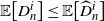 $\mathbb{E}\big[D_n^i\big]\leq \mathbb{E}\big[\widehat D_n^i\big]$
, where
 $\widehat D_n^i$
stands for the number of deactivations in this model while
 $\widehat N_n(t)+\widehat M_n(t)=i$
. In what follows we will give an idea of why
 $\mathbb E\big[\widehat D_n^i\big]=O\big(i^{-1/2}\big)$
, implying that
 $\mathbb E[ D_n]=O\big((\!\log n)^{1/2}\big)$
, and hence proving (4.3).
The details of the proof, which are unfortunately quite tedious, can be found in the proofs of [Reference Blath, González-Casanova, Kurt and Wilke-Berenguer1, Lemmas 4.10 and 4.11]. In the following, suppose that
 $c_1=c_2=1$
for the sake of simplicity.
Fix
 $i\geq 2$
. The variables
 $\widehat D_n^i$
tend to take higher values when coalescences are not permitted; we focus on this case. Thus, suppose that at time t,
 $\widehat N_n(t)+\widehat M_n(t)$
reaches i, with
 $\widehat N_n(t{-})=\lfloor\sqrt {i}\rfloor+1\geq\sqrt {i+1}$
. This means that
 $\widehat N_n(t)=\lfloor\sqrt i\rfloor\leq\sqrt i$
. Reactivations are then needed to allow a new coalescence. Conditional on this configuration, the probability that
 $\widehat D_n^i$
equals 0 is equivalent to
 \begin{equation*}\frac{i-\lfloor\sqrt i\rfloor}{i}\times\frac{\binom{\lfloor\sqrt i\rfloor}{2}}{\binom{\lfloor\sqrt i\rfloor}{2}+\lfloor\sqrt i\rfloor}\sim1-\frac{3}{\sqrt{i}\,}\,=\!:\,p_i.\end{equation*}
This corresponds approximately to the probability of one reactivation, followed by one coalescence, before one deactivation. So, we have the almost sure bound
 $\widehat D_n^i\leq\sum_{j=0}^{G^i-1}\Delta_j$
, where
 $G^i$
is a geometric random variable with parameter
 $p_i$
, and the
 $\Delta_j$
give the number of deactivations between each visit of the state
 $\lfloor\sqrt i\rfloor$
. The time when coalescence is not allowed is stochastically bounded from above by the time that a random walk that goes up one unit at rate
 $i-\sqrt{i}$
(rate at of a reactivation) and down at rate
 $\sqrt{i}$
(rate of a deactivation), started at zero, spends below level
 $\sqrt i$
. The random walk has ballistic speed of order i. In particular, it reaches the level
 $\sqrt{i}$
after
 $\sqrt{i}/i=1/\sqrt{i}$
units of time on average. During the period in which coalescence events are not allowed there are always less than
 $\sqrt{i}$
plants, each of which deactivates at rate
 $c_1({=}1)$
. Then, we conclude that, for any j,
 $\mathbb E\big[\Delta_j\big]\leq\frac{1}{\sqrt{i}}\cdot \sqrt{i}=1$
. This uniform bound implies that
 $\mathbb{E}\big[\widehat D_n^i\big]\leq \mathbb{E}[G^i-1]\mathbb{E}[\Delta_1]=O\!\left(\frac{1}{\sqrt i}\right)$
, since
 $\mathbb E[G^i-1]\sim\frac{3}{\sqrt i}$
.
4.2. The inactive length
Consider the inactive length defined in (1.5).
Theorem 4.2. Consider the seed bank coalescent starting with n plants and no seeds. Then,
 \begin{equation*}\lim_{n\rightarrow\infty}\frac{I_n}{\log n}=\frac{2c_1}{c_2} \quad {in\ probability.}\end{equation*}
Proof.Divide
 $I_n$
in two parts,
 $I^1_n=\int_0^{\theta_n}M_n(t) \, \text{d} t$
and
 $I^2_n=\int_{\theta_n}^{\sigma_n}M_n(t) \, \text{d} t$
. It is easy to prove that
 ${I^1_n}/{\log n}$
converges to 0 in probability by observing that, almost surely,
 $I^{1}_n\leq M_n({\theta_n})\cdot\theta_n$
, and using Proposition 3.1.
To study
 $I^2_n$
, we approximate it by the accumulated time for the
 $M_n({\theta_n})$
seeds to activate, namely
 $\tilde I^{2}_n=\sum_{k=1}^{M_n({\theta_n})} {e_k} / {c_2}$
, where the
 $e_k$
are i.i.d. standard exponential random variables. The asymptotics of this random variable are easily obtained by proceeding in two steps, similar to the proof of Proposition 2.2. First, by Proposition 3.1, we have
 $M_n(\theta_n)/\log n\to 2c_1$
in probability. Second, by denoting
 $G_n(t)=\sum_{k=1}^{\lfloor t\log n\rfloor}{e_k} / {c_2}$
, we get
 \begin{equation*}\lim_{n\to\infty}\dfrac{G_n(t)}{\log n} =\dfrac{t}{c_2}\end{equation*}
in
 $L^2$
. By observing that
 $\tilde I^2_n=G_n(M_n(\theta_n)/\log n)$
, we obtain the desired result,
 \begin{equation*}\lim_{n\rightarrow\infty}\frac{\tilde I^2_n}{\log n}=\frac{2c_1}{c_2} \quad \text{in probability.}\end{equation*}
Finally, the difference between
 $I^{2}_n$
and
 $\tilde I^{2}_n$
can be bounded by
 $I_{N_n(\theta_n)}+I_{M_n(\theta_n)}$
. Indeed, the variable
 $I_{N_n(\theta_n)}$
bounds the inactive length resulting from the plants present at time
 $\theta_n$
, and the variable
 $I_{M_n(\theta_n)}$
bounds the inactive length resulting from the seeds present at time
 $\theta_n$
that activate and deactivate again. Its expectation is clearly of order
 $\log\log n$
. This can be seen by repeating the earlier arguments of this proof.
5. Sampling formula
Consider the seed bank coalescent at time
 $\theta_n$
and go back through the active part of the genealogical tree until time zero when there are n active lineages and zero inactive lineages. During this period of time we observe
 $n-N_n(\theta_n)$
events divided into two types: branching inside one lineage (corresponding to a coalescence) and the appearance of a new lineage (corresponding to a deactivation). When there are k lineages, the probability that a branching event occurs is
 \begin{equation*}\frac{\binom{k+1}{2}}{\binom{k+1}{2}+c_1(k+1)}=\frac{k}{k+2c_1},\end{equation*}
whereas the probability that a new lineage appears is
 ${2c_1} / ({k+2c_1})$
. This observation leads to a connection with the classical Hoppe’s urn and the Chinese restaurant process (with parameter
 $2c_1$
), which are the key tools to prove Ewens’ sampling formula for the law of the allele frequency spectrum in the neutral model, see [Reference Durrett7, Section 1.3]. However, in our case, the initial configuration is made of a random number
 $N_n({\theta_n})$
of tables (old lineages) with one client in each. By applying results of [Reference Watterson18], we can obtain a conditional sampling formula corresponding to observing a certain configuration of lineages that passed through the seed bank and lineages that did not deactivate (until time
 $\theta_n$
).
Now, let
 $k\leq n$
be a positive integer; we define the sets
 $A(k,n) = \big\{a_i,b_i\geq 0, i\in[n] \,:$
 $ \sum_{i=1}^{n}a_i=k \mbox{ and } \sum_{i=1}^{n}i(a_i+b_i)=n \big\}$
and
 $\bar A(k,n) = \big\{a_i\geq 0, i\in[n] \,:\, \sum_{i=1}^{n}a_i=k $
and
 $\sum_{i=1}^{n}ia_i\leq n \big\}$
. From [Reference Watterson18, Eq.(3.3.2)], we obtain the next theorem.
Theorem 5.1. Let
 $O_i$
be the number of ‘old’ blocks of size i (i.e. active blocks of size i at time
 $\theta_n$
) and let
 $R_i$
be the number of ‘recent’ blocks of size i (i.e. inactive blocks of size i at time
 $\theta_n$
). Then
 \begin{align} \mathbb{P}\!\left( O_1=a_1,\dots,O_n\right. & = \left. a_n,R_1=b_1,\dots,R_n=b_n\mid N_n({\theta_n})\right)\nonumber\\ & \overset{\text{a.s.}} = \dfrac{(n-N_n({\theta_n}))!N_n({\theta_n})!}{(N_n({\theta_n})+2c_1)_{(n-N_n({\theta_n}))}}\prod_{i=1}^n \dfrac{1}{a_i!} \prod_{j=1}^n \dfrac{1}{b_j!}\left(\dfrac{2c_1}{j}\right)^{b_j},\end{align}
with
 $ (a_i,b_i)_{i\in[n]}\in A(N_n(\theta_n),n)$
.
Here, the notation
 $x_{(n)}$
stands for the ascending factorial, i.e.
 $x_{(n)}=x(x+1)\dots(x+n-1)$
.
Remark 5.1. From the latter result and Proposition 3.1, we can obtain an approximate unconditioned sampling formula for large n,
 \begin{align*} &\mathbb{P}\!\left(O_1=a_1,\dots,O_n=a_n,R_1=b_1,\dots,R_n=b_n\right) \\ &=\int_0^{\infty}\mathbb{P}\big( O_1=a_1,\dots,O_n=a_n,R_1=b_1,\dots,R_n=b_n \mid N_n({\theta_n})=\lfloor z\log n\rfloor\big) \\ & \qquad \quad \times \mathbb{P}(N_n({\theta_n})=\lfloor z\log n\rfloor) \, \text{d} z \\ & \sim \prod_{i=1}^n \dfrac{1}{a_i!} \prod_{j=1}^n \dfrac{1}{b_j!}\left(\dfrac{2c_1}{j}\right)^{b_j} \\ & \quad \times \int_0^\infty\frac{\Gamma(n-z\log n+1)\Gamma(z\log n+1)\Gamma(z\log n+2c_1)}{\Gamma(n+2c_1)}.\frac{4c_1c_2}{z^2}e^{-\frac{4c_1c_2}{z}}dz , \end{align*}
which does not depend on the non-observable variable
 $N_n(\theta_n)$
. Observe that our sampling formula does not make a statement on allele frequencies, but on block frequencies of active and inactive blocks at time
 $\theta_n$
.
The variables
 $O_i$
and
 $R_i$
can be inferred if we are capable of deciding if a present individual has visited the seed bank or not. This seems hard, since deactivation can be treated similarly to mutations from the mathematical point of view, but, as opposed to mutations, they do not leave tractable evidence. Furthermore, our result presents a snapshot of the partition at a random time, not at a deterministic one. For these reasons it seems too optimistic to believe that this study provides a possible method of estimating the parameters of the seed bank model.
From (5.1), we obtain the probability-generating function of the old and recent blocks.
Corollary 5.1. Let
 $O_1, \ldots, O_n, R_1, \ldots, R_n$
be random variables with joint density given by (5.1). Then, their (conditional) probability-generating function is
 \begin{align} \mathbb{E}\!\left[\prod_{i=1}^n t_i^{O_i} \prod_{j=1}^n s_j^{R_j} \mid N_n({\theta_n})\right] & = \dfrac{(n-N_n({\theta_n}))!N_n({\theta_n})!}{(N_n({\theta_n})+2c_1)_{(n-N_n({\theta}_n))}}\nonumber\\&\quad \times \sum_{\substack{a_1, \ldots, a_n, b_1, \ldots, b_n\in A(N_n(\theta_n),n)}}\prod_{i=1}^n\dfrac{(t_i)^{a_i}}{a_i!}\prod_{j=1}^n\dfrac{1}{b_j!}\left(\frac{2c_1s_j}{j}\right)^{b_j}.\end{align}
Following the idea of [Reference Watterson18] we use two artificial variables,
 $u\in({-}1,1)$
and
 $v\in({-}1,1)$
. They will help us to rewrite (5.2) in a simpler way. First, observe that, for
 $(a_i,b_i)\in A(k,n)$
,
 \begin{equation*} \prod_{i=1}^n \big(uv^i\big)^{a_i} \prod_{j=1}^n \big(v^j\big)^{b_j}=u^{\sum_{i=1}^n a_i} v^{\sum_{i=1}^n i(a_i+b_i)}=u^kv^n .\end{equation*}
Now let
 $c_{k,n}$
be the multiplying coefficient of
 $u^kv^n$
in
 $\exp\!\left\lbrace \sum_{i=1}^n uv^it_i+\sum_{j=1}^\infty \frac{2c_1}{j}s_jv^j\right\rbrace $
. We can rewrite (5.2) as
 \begin{align} \mathbb{E}\!\left[\prod_{i=1}^n t_i^{O_i} \prod_{j=1}^n s_j^{R_j} |N_n({\theta_n})\right]=\dfrac{(n-N_n({\theta_n}))!N_n({\theta_n})!}{(N_n({\theta_n})+2c_1)_{(n-N_n({\theta}_n))}}c_{N_n({\theta}_n),n}.\end{align}
From this relation, we obtain the probability-generating function of the lineages that have not gone through the seed bank at time
 $\theta_n$
.
Corollary 5.2. Let
 $O_i$
be the number of ‘old’ blocks of size i (i.e. active blocks of size i at time
 $\theta_n$
). Then, the joint probability-generating function of
 $O_1,O_2, \ldots, O_n$
is
 \begin{align} \mathbb{E}\!\left[\prod_{i=1}^n t_i^{O_i} \mid N_n({\theta_n})\right]=\sum_{a_1, \ldots, a_n\in\bar{A}(N_n({\theta_n}),n)}\dfrac{N_n({\theta_n})!}{a_1!a_2! \cdots a_n!}t_1^{a_1}t_2^{a_2} \cdots t_n^{a_n}\dfrac{\binom{2c_1+n-z-1}{n-z}}{\binom{2c_1+n-1}{n-N_n{\theta_n}}} ,\end{align}
where
 $z={\sum_{i=1}^nia_i}.$
Proof.First, we will write explicitly the term
 $c_{k,n}$
when
 $s_j=1$
for all j. Observe that
 \begin{align*} \exp\!\left\lbrace \sum_{i=1}^n uv^it_i+\sum_{j=1}^\infty\frac{2c_1}{j}v^j\right\rbrace & = (1-v)^{-2c_1} \exp\!\left\lbrace u\sum_{i=1}^{n} v^it_i\right\rbrace \\ & = (1-v)^{-2c_1}\sum_{k=0}^{\infty}\dfrac{\left[ u\sum_{i=1}^{n} v^it_i\right] ^{k}}{k!}.\end{align*}
This implies that the coefficient of
 $u^k$
in the latter expression is
 \begin{align*}\dfrac{\left[ \sum_{i=1}^{n} \big(v^it_i\big)\right] ^{k}}{k!}(1-v)^{-2c_1}=&\dfrac{\left[ \sum_{i=1}^{n} \big(v^it_i\big)\right] ^{k}}{k!}\left( \sum_{j=0}^{\infty} \binom{2c_1+j-1}{j}v^j\right).\end{align*}
We now need to find the coefficient of
 $v^n$
in the latter expression. First, observe that
 \begin{align*}\left[ \sum_{i=1}^{n} \big(v^it_i\big)\right] ^{k}=\sum_{{a_1+ \cdots +a_n=k}} \dfrac{k!}{a_1!a_2! \cdots a_n!}t_1^{a_1}t_2^{a_2} \cdots t_n^{a_n}v^{z} ,\end{align*}
where
 $z={\sum_{i=1}^nia_i}$
. For
 $z\leq n$
, the coefficient of
 $v^{n-z}$
in the expression
 \begin{equation*}\left( \sum_{j=0}^{\infty} \binom{2c_1+j-1}{j}v^j\right)\end{equation*}
is
 $\binom{2c_1+n-z-1}{n-z}$
. So,
 \begin{align*} c_{k,n} =\dfrac{1}{k!}\sum_{a_1, \ldots, a_n\in\bar A(k,n)} \dfrac{k!}{a_1!a_2! \cdots a_n!}t_1^{a_1}t_2^{a_2} \cdots t_n^{a_n}\binom{2c_1+n-z-1}{n-z}.\end{align*}
Thus, replacing
 $c_{N_n({\theta}_n),n}$
and
 $s_j=1$
for all j in (5.3), we have the result.
From the previous corollary we obtain the joint distribution of the lineages which have not gone through the seed bank at time
 $\theta_n$
:
 \begin{align*} \mathbb{P}\big( O_1=a_1, \ldots, O_n=a_n \mid N_n({\theta_n})\big) \overset{\text{a.s.}} = \frac{N_n({\theta_n})!}{a_1!a_2!\cdots a_n!}\frac{\binom{2c_1+n-z-1}{n-z}}{\binom{2c_1+n-1}{n-N_n({\theta_n})}}\end{align*}
when
 $a_1,\dots,a_n\in\bar A(N_n(\theta_n),n)$
.
Now, by taking
 $t_i=t^i$
and
 $s_j=1$
for all
 $i,j\in[n]$
in (5.3), and finding the corresponding coefficient
 $c_{N_n({\theta}_n),n}$
, we obtain the conditional probability-generating function of the number of lineages at time zero that have not been through the seed bank until time
 $\theta_n$
,
 \begin{align*} \mathbb{E}\!\left[ t^{\sum_{i=1}^niO_i} \mid N_n({\theta_n})\right] = \sum_{z=N_n({\theta_n}) }^nt^z \dfrac{\binom{2c_1+n-z-1}{n-z}\binom{z-1}{z-N_n({\theta_n})}}{\binom{2c_1+n-1}{n-N_n({\theta_n})}}.\end{align*}
Finally, from (5.3), by taking
 $t_i=1$
for all
 $i\in[n]$
, and from (5.4), we can find the conditional expectations of
 $O_j$
and
 $R_j$
for all
 ${j=1,2, \ldots, n-N_n({\theta_n})}$
:
 \begin{align*} \mathbb{E}\!\left[ O_j \mid N_n({\theta_n})\right] & = N_n({\theta_n})\dfrac{\binom{2c_1+n-j-1}{n-j-N_n({\theta_n})+1}}{\binom{2c_1+n-1}{n-N_n({\theta_n})}} , \\[4pt] \mathbb{E}\!\left[ R_j \mid N_n({\theta_n})\right] & = \frac{2c_1}{j}\dfrac{\binom{2c_1+n-j-1}{n-j-N_n({\theta_n})}}{\binom{2c_1+n-1}{n-N_n({\theta_n})}}.\end{align*}
Funding information
This project was partially supported by CoNaCyT grant FC-2016-1946 and UNAM-PAPIIT grant IA103820.
Competing interests
There were no competing interests to declare which arose during the preparation or publication process of this article.