NOMENCLATURE
- T
-
actual thrust of propeller
- Tr
-
required thrust of propeller
- Vs
-
horizontal flight speed of aircraft
- Q
-
torque of propeller
- ρ
-
air density
- Z
-
number of blades
- CL
-
lift coefficient
- CD
-
drag coefficient
- c
-
aerofoil chord length (m)
- Γ
-
concentrate circulation
- V*
-
total inflow speed (m/s)
- V a
-
axial inflow velocity (m/s)
- Vt
-
tangential inflow velocity (m/s)
- u* a
-
induced axial velocity (m/s)
- u* t
-
induced tangential velocity (m/s)
- λ
-
Lagrange multiplier
- KT
-
thrust coefficient based on blade tip speed
- KQ
-
torque coefficient based on blade tip speed
- Js
-
advance ratio
- η
-
propeller efficiency (%)
- ω
-
propeller angular velocity (rad/s)
- N
-
propeller revolutions per minute (RPM)
- R
-
propeller radius (m)
- EA
-
expanded area
- Eo
-
disk area
1.0 INTRODUCTION
In recent years, the interest in stratospheric aircrafts has been increased considerably. Their long endurance, low energy consumption and high security make stratospheric aircrafts attractive for both military and civilian applications(Reference Colozza and Dolce1,Reference Jamison, Sommer and Porche2) . Propellers are widely used on aircrafts as a source of thrust(Reference Ilieva, Páscoa, Dumas and Trancossi3,Reference Liu, Duan and Ma4) . The increased propulsion efficiency of the propeller is of great importance in aviation to reduce energy consumption and improve cruising periods. Although flight performance can be improved through the implementation of solar cells on the deck of the aircraft, it is still limited in the absence of sunlight. Significant propulsive performance improvements of propellers can be achieved through the optimization design due to the flight environment where the air density is much lower and the advance velocity of aircraft is extremely slow (about 10–30 m/s), which makes it a big challenge to design efficient propeller propulsions for stratospheric aircrafts(Reference Tang, Liu, Chen and Guo5). Hence, the focus on improving the propulsive efficiency is a top priority.
There are two main propeller geometrical adjustments that could be made to improve the propeller performance(Reference Nie6). Firstly, different aerofoil cross-sectional shapes will affect the lift coefficients at different altitudes, affecting the propeller efficiencies under different conditions(Reference Koch7,Reference Ma and Liu8) . Secondly, the variation of blade pitch angles and chord lengths will also alter the propulsive efficiency(Reference D'Angelo, Berardi and Minisci9). The VLM method(Reference Lerbs10,Reference Coney11) has been widely used in the design process of propellers for many years. It is capable of calculating the prime efficiency of an air propeller given wings with high aspect ratios. Coney(Reference Coney11) suggested an algorithm to determine the optimal radial distributions of circulation for propellers, which was incorporated into the propeller wake model for lightly to moderately loaded propellers. Epps et al(Reference Epps, Chalfant, Kimball, Techet and Chryssostomidis12) implemented Coney's generalised propeller optimiser and created an off-design analysis routine to predict the performance curve for a given propeller design. Epps(Reference Epps and Kimball13) corrected the classical wake model used on moderately loaded propellers and identified a new wake model representing each panel as a constant-pitch vortex sheet. However, the methods mentioned above did not consider the aerodynamic properties of the aerofoil, such as the Reynolds number and Mach number at radial locations. These properties should be taken into consideration for high-altitude propellers.
The focus of this paper is a novel method based on Coney's optimiser(Reference Coney11) to optimise the blade chord and pitch distributions and obtain the desired circulation at the angle-of-attack where the aerofoil has a maximum lift-drag ratio. The pitch is calculated by the both values of inflow and desired angles-of-attack. The chord is also optimised by using the appropriate circulation, total inflow speed determined by Coney's method, and a proper lift coefficient where the lift-drag ratio is maximum. This approach results in a higher efficiency than prescribing chord arbitrarily. Furthermore, the effects of the Reynolds and Mach numbers, coupled with the aerofoil aerodynamic data from the CFD method, will be presented in this paper. The information will provide the ideal propeller characteristics with results close enough to CFD methods. The relation between the optimal efficiency and the design parameters of the propellers are obtainable. The design parameters include the number of blades, blade radius and rotation speed.
The paper is organised into five main sections. In Section 2, the algorithm for the propeller optimiser will be described, followed by the analysis of the aerodynamic characteristics of the S1223 aerofoil in Section 3. After which, the validation of the used method using the CFD method will be described in Section 4 and the analysis of the optimum efficiency and design parameters of propellers will be analysed in Section 5. Lastly, we will draw conclusions on the computational methods and propeller characteristics at high altitude.
2.0 THE IMPROVED ALGORITHM OF PROPELLER OPTIMISER
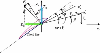
The relative velocity and forces on the propeller aerofoil are shown on the basis of VLM in Fig. 1, where ωr is the relative velocity of propeller and Vt
, Va
and V
0 are the tangential, axial and composite inflow velocity, respectively. During the course of the propeller optimization design, the tangential inflow velocity was assumed to be negligible. u*
t
and u*
a
are the tangential and axial induced velocity, respectively, which can be calculated using tangential and axial induced factors
 $\bar{u}_t^*(m,i),\bar{u}_a^*(m,i), m,i = 1 \sim M$
(Reference Wrench14). V* is the composite velocity which takes into consideration the induced velocity. ϑ is the pitch angle, α is the angle-of-attack of the aerofoil. β is the aerodynamic pitch angle caused by Vt
and Va
• β
i
is the aerodynamic pitch angle that is a function of induced velocity. Fi
, Fv
and F are the inviscid lift force, viscous force and composite force, respectively. T
(i) and D
(i) are the actual thrust and drag of blade aerofoil.
Velocity, angle and force diagram of blade aerofoil.

The propeller has Z blades. Each blade was divided into M segments (M = 15)(Reference Epps, Chalfant, Kimball, Techet and Chryssostomidis12). The concentrate circulation Γ(i) on each segment is a key variable that needs to be optimised.
Assuming the Z blades are identical, the total thrust T and torque Q on the propeller(Reference Epps, Chalfant, Kimball, Techet and Chryssostomidis12) are:
 $$\begin{equation}
T = Z\int_{{r_h}}^R {\left[ {{F_i}\cos {\beta _i} - {F_v}\sin {\beta _i}} \right]} dr,
\end{equation}$$\\
 $$\begin{equation}
Q = Z\int_{{r_h}}^R {\left[ {{F_i}\sin {\beta _i} + {F_v}\cos {\beta _i}} \right]} rdr
\end{equation}$$
Based on the trigonometric relations between β i and the blade, the total thrust and torque on the propeller are:
 $$\begin{equation}
T = \rho Z\sum\limits_{i = 1}^M {\{ [wr + {V_t} + {u_{t(i)}}^*] \cdot {\Gamma _{(i)}} - \frac{1}{2}} {V_{(i)}}^*{C_{D(i)}}{c_{(i)}}[{V_a} + {u_{a(i)}}^*]\} \Delta r,
\end{equation}$$\\
 $$\begin{equation}
Q = \rho Z\sum\limits_{i = 1}^M {\{ [{V_a} + {u_{a(i)}}^*] \cdot {\Gamma _{(i)}} + \frac{1}{2}} {V_{(i)}}^*{C_{D(i)}}{c_{(i)}}[wr + {V_t} + {u_{t(i)}}^*]\} r\Delta r,
\end{equation}$$
 $\bar{u}_t^*\& \bar{u}_a^*$
in wake alignment model(Reference Epps and Kimball13). u*
a
and u*
t
are formulated as:
 $$\begin{equation}
u{^*_{a{(m)}}} = \sum\limits_{i = 1}^M {\Gamma (i)\bar{u}_a^*} (m,i) ,
\end{equation}$$\\
 $$\begin{equation}
u{^*_{t{(m)}}} = \sum\limits_{i = 1}^M {\Gamma (i)\bar{u}_t^*} (m,i)
\end{equation}$$
The propulsive efficiency of propeller can be written as:
 $$\begin{equation}
\eta = \frac{{T{V_s}}}{{Q\omega }},
\end{equation}$$
where Vs is the flight speed of aircraft and ω is the angular velocity of propeller rotation. The flight speed of aircraft Vs is assumed to be equivalent to the axial inflow velocity Va .
To obtain the maximum efficiency η, Coney(Reference Coney11) employs the method of Lagrange multiplier from variational calculus. He forms an auxiliary function:
 $$\begin{equation}
H = Q + \lambda (T - {T_r})
\end{equation}$$
If, when T = Tr , min H = min Q.
For the minimum H, the derivatives with respect to the unknowns are assumed negligible.
 $$\begin{equation}
\frac{{\partial H}}{{\partial {\Gamma _{(i)}}}} = 0\quad {\rm{for}}\;i = 1...M,
\end{equation}$$\\
 $$\begin{equation}
\frac{{\partial H}}{{\partial \lambda }} = 0
\end{equation}$$
From Equations (9) and (10), we can obtain a system of M+1 nonlinear equations for M+1 unknown variables. For solving the optimised circulation distribution and flow parameters, these systems can be linearised by freezing flow parameters
 $\{ {{\rm{u}}_a^*,{\rm{u}}_t^*,{\rm{\bar{u}}}_a^*,{\rm{\bar{u}}}_t^*,{V^*},\frac{{\partial {V^*}}}{{\partial T}},\lambda } \}$
. More details can be found in Coney(Reference Coney11) and Epps et al(Reference Epps, Chalfant, Kimball, Techet and Chryssostomidis12).
Based on the required thrust of the propeller, the number of blades, the propeller radius, the rotation speed, and the airspeed of aircraft, the ideal circulation distribution can be obtained using Coney's optimization method.
c (i) can be optimised by making every aerofoil section under the condition of maximum lift-drag ratio (L/D)max. c (i) is deduced as:
 $$\begin{equation}
{c_{(i)}} = \frac{{2{\Gamma _{(i)}}}}{{V_{(i)}^* \cdot {C_{L(i)\_{{\left( {L/D} \right)}_{{\rm{max}}}}}}}}
\end{equation}$$
Substituting Equation (11) and
 ${C_{D(i)\_{{( {L/D} )}_{{\rm{max}}}}}}$
into Equations (3) and (4) and rewriting them:
 $$\begin{equation}
T = \rho Z\sum\limits_{i = 1}^M {(wr + {V_t} + u_{t(i)}^* - \frac{{{V_a} + u_{a(i)}^*}}{{{{\left( {L/D} \right)}_{{\rm{max}}}}}}) \cdot {\Gamma _{(i)}}} \Delta r,
\end{equation}$$\\
 $$\begin{equation}
Q = \rho Z\sum\limits_{i = 1}^M {({V_a} + u_{a(i)}^* + \frac{{wr + {V_t} + u_{t(i)}^*}}{{{{\left( {L/D} \right)}_{{\rm{max}}}}}}) \cdot {\Gamma _{(i)}}} r\Delta r
\end{equation}$$
According to Equations (12) and (13), the systems can be linearised by freezing flow parameters
 $\{ {u_a^*,u_t^*,\bar{u}_a^*,\bar{u}_t^*,{C_{L(i)\_{{( {L/D} )}_{{\rm{max}}}}}},{C_{D(i)\_{{( {L/D} )}_{{\rm{max}}}}}},{{( {L/D} )}_{{\rm{max}}}},\lambda } \}$
.
Before updating (L/D)max, c (i) should be computed by using Equation (14):
 $$\begin{equation}
{c_{(i)}} = \frac{{2{\Gamma _{(i)}}}}{{V_{(i)}^* \cdot {{\hat{C}}_{L(i)\_{{\left( {L/D} \right)}_{{\rm{max}}}}}}}},
\end{equation}$$
where V*(i) can computed as:
 $$\begin{equation}
V_{(i)}^* = \sqrt {{{({V_a} + u_{a(i)}^*)}^2} + (wr + {V_t} + u_{t(i)}^*)}
\end{equation}$$
Note that
 ${\hat{C}_{L(i)\_{{( {L/D} )}_{{\rm{max}}}}}}$
in equation (14) is a frozen value. The Reynolds number Re(c
(i)) and the Mach number Ma(c
(i)) can be attained by applying c
(i) into Equation (14):
 $$\begin{equation}
{\rm{R}}{{\rm{e}}_{(i)}} = \frac{{\rho \cdot {c_{(i)}} \cdot V_{(i)}^*}}{\mu },
\end{equation}$$\\
 $$\begin{equation}
{\rm{M}}{{\rm{a}}_{(i)}} = \frac{{V_{(i)}^*}}{c},
\end{equation}$$
The Reynolds number and Mach number obtained from Equations (16) and (17), along with aerodynamic properties of the aerofoil, will determine a new maximum lift-drag ratio, (L/D)max. (The aerodynamic properties will be discussed in Section 3.) New values of the lift coefficient,
 ${C_{L(i)\_{{( {L/D} )}_{{\rm{max}}}}}}$
, drag coefficient,
 ${C_{D(i)\_{{( {L/D} )}_{{\rm{max}}}}}}$
, and the angle-of-attack at each aerofoil section,
 ${\alpha _{(i)\_{{( {L/D} )}_{{\rm{max}}}}}}$
, will also be updated according to the new maximum lift-drag ratio.
As is shown in Fig. 1, β i can be determined by:
 $$\begin{equation}
{\beta _{i(i)}} = \arctan \frac{{{V_a} + u_a^*}}{{wr + {V_t} + u_t^*}}
\end{equation}$$
ϑ(i) is computed as:
 $$\begin{equation}
{\vartheta _{(i)}} = {\alpha _{(i)\_{{\left( {L/D} \right)}_{{\rm{max}}}}}} + {\beta _{i(i)}}
\end{equation}$$
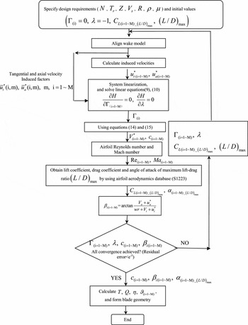
The flow chart for optimum propeller design is shown in Fig. 2.
Flow chart for optimum propeller design.

3.0 THE AERODYNAMIC CHARACTERISTICS OF S1223 AEROFOIL
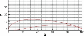
For the high-aspect-ratio blade, the aerodynamic characteristics of a two dimension aerofoil is very important for the three dimension propulsive performance. In Tang et al(Reference Tang, Liu, Chen and Guo5), the Reynolds numbers of high-altitude propellers range from 105 to 106, which may be defined as the lower range of Reynolds numbers. Aerofoil S1223 has a Reynolds number that falls within the defined low range(Reference Ma and Liu8). Therefore, this aerofoil was chosen for this paper. The thrust of the propeller at a high altitude is small compared to that just above ground, reducing the structural requirements of the propeller. Furthermore, Tang has performed a wind tunnel experiment for high-altitude propellers using aerofoil S1223. Thus, the structural integrity of the aerofoil is not a main concern in the design of high-altitude propellers. The contour of aerofoil S1223 is shown in Fig. 3.
Contour of aerofoil S1223.

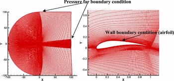
The aerodynamic characteristics of aerofoil S1223 fall in the regions of Reynolds number (Re = 3,000 ~ 2.0 × 10⁷), Mach number (Ma = 0.05 ~ 0.9) and angel of aerofoil (alpha = 0~16º). These properties will be used to obtain the accurate chord length and pitch angle distribution of propeller blades. The aerodynamic characteristics were calculated by CFD method (FLUENT). The mesh of aerofoil S1223 is shown in Fig. 4. The obtained aerodynamic data is assumed to be the database in the propeller optimization design.
The boundary condition and mesh used in FLUENT.

The calculation conditions of aerodynamic data are:
Mach number: 0.05, 0.1 ~ 0.9 (interval 0.1).
Reynolds number: 3 × 10⁴, 6 × 10⁴, 1.2 × 10⁵, 1.8 × 10⁵, 4.8 × 10⁵, 9.6 × 10⁵, 1.5 × 10⁶, 5.5 × 10⁶, 1.0 × 10⁷, 2.0 × 10⁷.
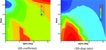
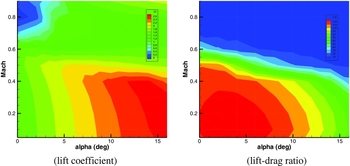
The lift coefficient and lift-drag ratio on Re = 30,000 and 2.0 × 10⁷ are shown in Figs 5 and 6.
The lift coefficient and lift-drag ratio on Re = 30,000.

The lift coefficient and lift-drag ratio on Re = 2.0 × 10⁷.

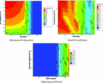
The maximum lift-drag ratio and ideal lift coefficient of maximum lift-drag ratio with variation of Reynolds number and Mach number are shown in Fig. 7. It is clearly seen that the maximum lift-drag ratio and ideal lift coefficient of maximum lift-drag ratio decline as the Mach number increases, especially when it exceeds the critical Mach of aerofoil S1223. The critical Mach number can be derived from Fig. 7, which shows that the value of optimal drag coefficient is increased dramatically when the Mach number exceeds 0.6. Also, the estimation method for the critical Mach of aerofoil can be found in Tang(Reference Basavaraj15).
The optimal lift-drag ratio, ideal lift coefficient and ideal drag coefficient of aerofoil S1223 under conditions of different Reynolds numbers and Mach numbers.

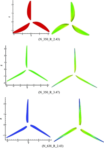
The propeller shape and pressure coefficient distribution of three propellers.

4.0 VALIDATION OF THE PROPELLER OPTIMIZATION METHOD
The propeller performances were analysed using the vortex lattice lifting line method (VLM) theory and the accurate aerofoil aerodynamic data was obtained by the CFD method. Moreover, the chord length and pitch angle distribution were gained through the maximum lift-drag ratio of the aerofoil.
To verify the capability of the improved method, three different propellers were calculated using the CFD method. The three propellers were obtained using the optimised method. The design conditions of propeller are:
Flight speed of aircraft: Vs = 20 m/s.
Required thrust of propeller: Tr = 484 N.
The numerical method used in this paper is the FLUENT 6.3.26 steady Reynolds-averaged Navieer-Stokes solver(16). The control equations were solved using density-based solver, single precision, second order in space. The flux type is Roe-FDS. The courant number is 5. A one-equation Spalart-Allmaras (S-A) model(Reference Spalart and AllMarchas17) was used.
The fluid boundary is 50 times longer than blade length. The fluid mesh is unstructured mesh (the cell number is about 2.34 million). The fluid field was divided into an outer region and an inner region. The motion of the propeller uses the moving reference frame on the inner region, which attaches with the propeller. The boundaries are the pressure far-boundary condition.
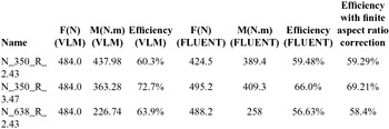
Comparing the results obtained from the CFD method and the improved VLM method, we can see that the error of the propeller is about 6%. There is no standard model for high-altitude propellers(Reference Morgado, Abdollahzadeh, Silvestre and PÁscoa18). The error from the VLM can be validated using the CFD method. The CFD results are assumed to have small errors. The VLM error of 6% is relative to the CFD results. In addition, an error of 6% is reasonable since the error using the JBLADE method(Reference Morgado, Abdollahzadeh, Silvestre and PÁscoa18) exceeds 10%. The VLM has been verified using 4119 and 4381 propellers by Epps and Kimball(Reference Epps and Kimball13).
As for propeller blades, they have a finite span and the performance of those finite-span blades differ significantly from the performance of the corresponding two-dimensional aerofoils. The finite aspect ratio correction(Reference Epps and Kimball13,Reference Anderson19) is:
 $$\begin{equation}
C_{L\alpha }^{{\rm{3}}D} = \frac{{C_{L\alpha }^{2D}}}{{1 + C_{L\alpha }^{2D}/(\pi {\rm{e}}AR)}}
\end{equation}$$
where C 3D Lα is the lift slope after the correction (3D aerofoil), C 2D Lα is the lift slope for an infinite blade (2D aerofoil), e is a span efficiency factor and AR is the aspect ratio of the blade. As is shown in Table 1, the finite aspect ratio correction would improve the accuracy of the propeller geometry and reduce the differences between the CFD and VLM results.
The efficiencies of three propellers using different methods

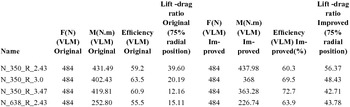
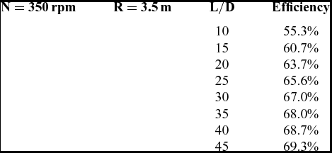
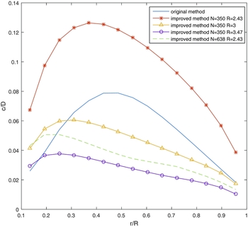
The improved VLM method can obtain the characteristics of different propellers. For the propulsion of aircraft, it is desirable to use low disk loading propellers (i.e., a lightly and moderately loaded propeller) that can obtain greater efficiency(Reference Ilieva, Páscoa, Dumas and Trancossi3). The propeller wake model of the improved VLM method is a regular helical slipstream. This wake model can be applied to lightly and moderately loaded propellers effectively. The performances using the original and improved methods are presented in Table 2. It is shown that the efficiency derived from the improved method is higher than that derived from the original method. As is shown in Table 3, if we fix the maximum lift-drag ratio (L/D)max term in Equations (12), (13) and prevent it from updating in the iterative process shown in Fig. 2, the efficiency performance is better with the increasing value of maximum lift-drag ratio, which means the maximum lift-drag ratio indeed contributes to the performance of the improved method. Lift-drag ratios at 75% radial position of the original and improved methods are also shown in Table 2. In the original method, the chord distribution is determined in advance. The chord distribution which has been given in Liu et al(Reference Liu, Duan and Ma4) is shown in Fig. 9. In the improved method, the chord distributions are optimised during the process of the algorithm presented in Fig. 2 and are also shown in Fig. 9.
The efficiencies of three propellers using different methods

Efficiency performances of specified propellers under different maximum lift-drag ratio situations

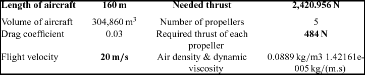
The size of stratosphere aircraft and needed thrust parameter

The chord distribution of propellers in the original and improved method.

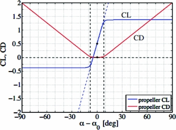
The lift and drag coefficient computed in the original method are shown in Fig. 10 and given by these equations:
 $$\begin{equation}
\begin{array}{@{}l@{}} {C_L}{\rm{ = }}{C_{L0}}{\rm{ + }}\frac{{d{C_L}}}{{d\alpha }}\Delta \alpha - \frac{{d{C_L}}}{{d\alpha }}(\Delta \alpha - \Delta {\alpha _{{\rm{stall}}}}) \cdot F(\Delta \alpha - \Delta {\alpha _{{\rm{stall}}}}) + \\ \frac{{d{C_L}}}{{d\alpha }}( - \Delta \alpha - \Delta {\alpha _{{\rm{stall}}}}) \cdot F( - \Delta \alpha - \Delta {\alpha _{{\rm{stall}}}}) \end{array}
\end{equation}$$\\
 $$\begin{equation}
\begin{array}{@{}l@{}} {C_D} = {C_{D0}} + A \cdot (\Delta \alpha - \Delta {\alpha _{{\rm{stall}}}}) \cdot F(\Delta \alpha - \Delta {\alpha _{{\rm{stall}}}}) + \\ A \cdot ( - \Delta \alpha - \Delta {\alpha _{{\rm{stall}}}}) \cdot F( - \Delta \alpha - \Delta {\alpha _{{\rm{stall}}}}) - 2A \cdot ( - \Delta {\alpha _{{\rm{stall}}}}) \cdot F( - \Delta {\alpha _{{\rm{stall}}}}) \end{array}
\end{equation}$$
 $\frac{{d{C_L}}}{{d\alpha }}$
is the lift curve slope, More details about the calculation of the lift and drag coefficient in the original method can be found in Epps and Kimball(Reference Epps and Kimball13).
Lift and drag coefficient versus net angle-of-attack.

By using Equation (11), the lift coefficient can be deduced as:
 $$\begin{equation}
{C_{L(i)}} = \frac{{2{\Gamma _{(i)}}}}{{V_{(i)}^* \cdot {c_{(i)}}}}
\end{equation}$$
Thus, the drag coefficient and the angle-of-attack during the process of the optimisation in the original method are determined by using Equations (21) and (22). The optimization algorithm in the original strategy can be obtained from Coney(Reference Coney11).
5.0 EFFICIENCY OPTIMISED BY RATE OF ROTATION, PROPELLER RADIUS AND BLADE NUMBER
In general, the length of stratosphere aircraft is about 150–200 m. The volume of the aircraft hull is about 300,000 m3. In this paper, we used the thrust needed on a stratosphere aircraft as the design conditions of a high-altitude propeller.
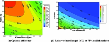
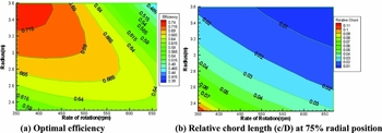
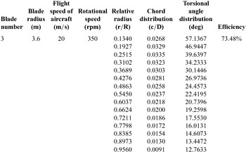
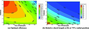
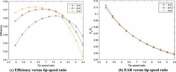
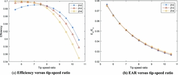
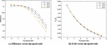
In this section, the optimum efficiency of propellers under the condition of different rate of rotation, propeller radius and blade number are analysed using the improved VLM method. The optimised characteristics, including efficiency and relative chord length with different parameters, are presented in Figs 11–13. It is shown that the chord length is decreased with the increasing number of blades at the specified thrust requirement. The propellers’ parameters with the maximum efficiency in Fig. 12 are shown in Table 5.
Z = 2, N = 350-670, R = 2.3–3.6.

Z = 3, N = 350–670, R = 2.3–3.6.

The propellers parameters with the maximum efficiency

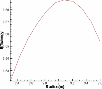
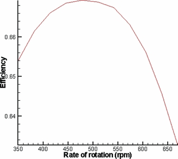
From the results shown in Figs 11–13, we can see that, at certain blade numbers and rates of rotation, the optimum efficiency has maximal value with the variation of the radius. Also, the optimum efficiency has maximal value when blade number and rate of rotation are certain. In design condition, the optimum efficiency of rate of rotation number N = 510 rpm and radius R = 2.69 m at blade number Z = 3 is shown in Figs 14 and 15 respectively.
Z = 4, N = 350–670, R = 2.3–3.6.

Rate of rotation number is 510 rpm.

The radius of blade is 2.69 m.

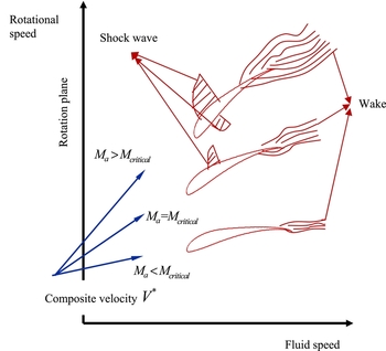
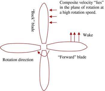
The optimum efficiency differences between different blade numbers are shown in Figs 16–18 (a). As is shown in Figs 16–18 (b), the expanded area ratios are almost constant, which means blade area has no effect on efficiency in the comparative study. It is clearly seen that the optimum efficiency goes up with the increase of the blade number when the tip-speed ratio is small, but as the tip-speed ratio increases, the result reverses. This is because as Z increases, blade-to-blade interaction induces performance decay and lowers the efficiency(Reference Felli, Camussi and Di Felice20). This is obvious when the advance ratio J is low and the rotation speed is relatively high. As in shown in Figs 19 and 20, when the propeller turns at a low speed, the orientation of the composite velocity V* is distant from the plane of rotation, but as rotation speed increases, the composite velocity V* “lies” in the plane of rotation. At a high rotation speed, if blades are too close, the strong interblade interaction is obvious, since the composite velocity V* of the “back” blade is affected by the wake of the “forward” blade. The composite velocity V* can flow between the blades but is affected by turbulence over the blades due to the wake. Also, viscous drag dominates at a very high rotation speed. These two factors reduce the efficiency at a high rotation speed. At a low rotation speed, the influence of blade-to-blade interaction is relatively small and negligible. The efficiency is then affected by other factors such as the circulation distribution, aerofoil characteristics and the number of blades.
The design radius is R = 2.7 m.

The design radius is R = 3 m.

The design radius is R = 3.2 m.

Aerofoil sections under different composite velocities(21).

“Forward” and “back” blade.

6.0 CONCLUSIONS
The paper proposes an improved method to design high-altitude propellers based on an algorithm of propeller optimisation, which is a fast and accurate propeller design method. The method determines the optimum propeller chord lengths and pitch angle through considering the variation of Reynolds numbers and Mach numbers at radial locations which are sensitive on high-altitude propellers. It can be a useful tool to analyse the relations between optimum efficiency and design parameters of propellers. Through the analysis of optimum efficiency of propellers under the condition of different rates of rotation, propeller radius, and blade number, the obtained distribution results of optimum efficiency with parameters can be used to select the high-altitude propellers in the initial design stage of a stratosphere aircraft.
APPENDIX A
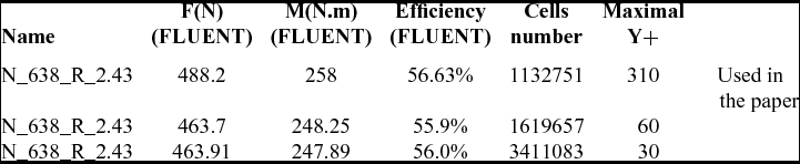
The mesh used in this paper is refined and analysed. The results are shown in Table A1:
Case: N_638_R_2.43 (VLM efficiency is 63.9%)

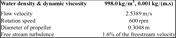
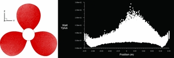
From the results, we can see that the mesh cell number and the Y+ (the boundary layer mesh) cannot affect the efficiency of the propeller considerably. The efficiency of the propeller is accurate when the mesh (cells number: 1132751, maximal Y+ = 310) is used in this paper. For verifying the accuracy of the CFD method, we can only find the experimental data of DTMB 4119 propeller(Reference Trejo, Terceño, Valle, Iranzo and Domingo22). The calculation conditions and discretisation of DTMB 4119 propeller when using CFD method is shown in Table A2 and Table A3. The CFD mesh (cell number: 2409890) of the DTMB4119 propeller is shown in Fig. A1.
The calculation conditions of DTMB 4119 propeller

Discretisation of DTMB 4119 propeller using CFD method

The CFD mesh of DTMB4119 propeller.

We have used different meshes (such as the refined wake region mesh and the boundary layer mesh), but the results of the CFD are almost the same. The results are shown in the Table A4.
Comparison of the results of DTMB 4119 propeller using the CFD method and the experiment