


1. Introduction
Thermal convection in a rapidly rotating system has been widely studied because of its interesting mathematical properties (Jones, Soward & Mussa Reference Jones, Soward and Mussa2000) and its relevance to the problems in geophysics and astrophysics. The investigation of the onset of linear convection is of fundamental importance, which can provide an invaluable guide for understanding the very complex behaviour in the nonlinear regime (Jones, Kuzanyan & Mitchell Reference Jones, Kuzanyan and Mitchell2009) and establishing asymptotic behaviour (Jones et al. Reference Jones, Soward and Mussa2000).
The Boussinesq approximation (Chandrasekhar Reference Chandrasekhar1961) has been widely used in buoyancy-driven convection because of its convenience through which density variations are neglected except in the buoyancy term of the momentum equation where the density is assumed to be linearly dependent on the temperature. Roberts (Reference Roberts1968) and Busse (Reference Busse1970) developed the local asymptotic theory of the onset of rapidly rotating convection in a Boussinesq sphere. The convection structure of columnar rolls with their axes aligned with the axis of rotation is properly characterized by the Roberts–Busse theory. However, their local theory of convection cannot predict the critical parameters, especially at small Prandtl numbers (Zhang Reference Zhang1992). The Roberts–Busse theory was further developed and the critical parameters given by the global theory of convection are in agreement with the numerical results (Yano Reference Yano1992; Jones et al. Reference Jones, Soward and Mussa2000; Dormy et al. Reference Dormy, Soward, Jones, Jault and Cardin2004). The prograde spiralling drifting columnar rolls modes (Hart, Glatzmaier & Toomre Reference Hart, Glatzmaier and Toomre1986; Zhang Reference Zhang1992) and inertial oscillation modes mainly occurring in the equatorial region (Zhang & Busse Reference Zhang and Busse1987; Zhang Reference Zhang1993, Reference Zhang1994; Busse & Simitev Reference Busse and Simitev2004) were discovered and analysed at small Prandtl numbers. It was found that the fundamental properties of convection are not substantially influenced by the aspect ratio of the spherical shell (Zhang Reference Zhang1992).
Nevertheless, there is usually a large density variation in the radial direction in stars and giant planets, so the Boussinesq approximation is no longer valid in these systems. Since more computing power is required for fully compressible equations, the sound-proof approaches were widely used for low-speed flows, such as the anelastic approximation (Ogura & Phillips Reference Ogura and Phillips1962; Gough Reference Gough1969), to save computational costs. The onsets of convection and nonlinear convection with large density variation in a rotating spherical geometry were investigated with the use of the anelastic equations (Gilman & Glatzmaier Reference Gilman and Glatzmaier1981; Glatzmaier & Gilman Reference Glatzmaier and Gilman1981; Verhoeven, Wiesehöfer & Stellmach Reference Verhoeven, Wiesehöfer and Stellmach2015). However, Drew, Jones & Zhang (Reference Drew, Jones and Zhang1995) investigated this problem at larger Taylor numbers and a broader range of Prandtl numbers and found that the critical Rayleigh number ( $Ra_{c}$) for convection onset becomes negative at small Prandtl number and large Taylor number. By replacing thermal diffusion with entropy diffusion in the anelastic model, Jones et al. (Reference Jones, Kuzanyan and Mitchell2009) showed that the critical Rayleigh number is always positive for convection onset.
Recently, studies have been performed to investigate the rotating compressible convection using the fully compressible equations. These studies have provided knowledge regarding the applicability of the anelastic approximation in the description of compressible convection in different regimes. The instability for rotating compressible convection in a plane layer geometry was investigated by Calkins, Julien & Marti (Reference Calkins, Julien and Marti2015b) for a unity Prandtl number. They compared the stability criteria of compressible and anelastic ideal gases and found that the critical parameters given by compressible equations approach those given by the anelastic equations in the adiabatic limit. However, for small Prandtl numbers and rapidly rotating cases Calkins, Julien & Marti (Reference Calkins, Julien and Marti2015a) found that the time derivative of the density reaches a non-negligible level, indicating that the anelastic approximation is not suitable. Verhoeven & Glatzmaier (Reference Verhoeven and Glatzmaier2018) investigated linear compressible convection within a Newtonian ideal gas in a rotating plane layer geometry, and found that the anelastic approach breaks down when the sound-crossing time of the computational domain exceeds the rotation time scale. Liu et al. (Reference Liu, Wan, Yan, Sun and Sun2019) studied the onset of fully compressible convection in a rapidly rotating spherical shell by linear stability analysis. A new quasi-geostrophic compressible mode was found at relatively small Prandtl numbers and the anelastic approximation in their system breaks down in the small- $Ra$ and large-
 $N_{\rho }$ regime, where
 $N_{\rho }$ denotes the number of density scale height.
The convective instabilities in rapidly rotating spheres and spherical shells have been well studied for Boussinesq fluids (Roberts Reference Roberts1968; Busse Reference Busse1970; Soward Reference Soward1977; Zhang Reference Zhang1992, Reference Zhang1994; Jones et al. Reference Jones, Soward and Mussa2000; Dormy et al. Reference Dormy, Soward, Jones, Jault and Cardin2004; Sánchez, García & Net Reference Sánchez, García and Net2016b; Zhang, Lam & Kong Reference Zhang, Lam and Kong2017), and rapidly rotating convection subject to large density stratification has been commonly studied within the anelastic approximation (Gilman & Glatzmaier Reference Gilman and Glatzmaier1981; Drew et al. Reference Drew, Jones and Zhang1995; Jones et al. Reference Jones, Kuzanyan and Mitchell2009). So far, the applicability of the anelastic approximation to compressible convection is still in debate and relevant studies using the unambiguous fully compressible equations are still rare. It has been shown that the anelastic approximation is no longer accurate for marginally stable convection in the rapidly rotating and small-Prandtl-number regime (Calkins et al. Reference Calkins, Julien and Marti2015a; Liu et al. Reference Liu, Wan, Yan, Sun and Sun2019). Further studies of the fully compressible convection modes are desirable. The fact that, hitherto, the physical mechanisms governing the onset of compressible convection in rapidly rotating spherical geometries have not been elucidated and that only a limited parameter region has been considered provides a motivation for the present work. In this study, the influence of the radius ratio on the onset of fully compressible convection in rotating spherical shells is investigated systematically. More importantly, we perform quantitative and qualitative analyses based on the linearized perturbation equations and the compressible Reynolds–Orr equation to gain a better physical understanding of the different modes, as well as the influence of the radius ratio.
The remainder of this study is organized as follows: the mathematical formulation of the problem is presented in § 2. In § 3, firstly, the influence of the radius ratio on the onset of convection based on the fully compressible equations is presented in detail. Secondly, the critical parameters at different radius ratios are discussed and compared for a wide range of parameters. Thirdly, the linear perturbation equations are employed to study the mechanical mechanisms for the different modes, as well as the influence of the radius ratio. Finally, for different radius ratios, a kinetic energy analysis based on the Reynolds–Orr equation is presented to reveal the flow instability mechanisms for the columnar mode and the quasi-geostrophic compressible mode. In § 4, we summarize the findings and conclude the paper.
2. Mathematical formulation of the problem
A spherical shell of depth  $d=r_{o}-r_{i}$ is considered to be filled with ideal gas rotating uniformly with a constant angular velocity of
 $\varOmega$, where
 $r_{o}$ and
 $r_{i}$ denote the radius of the spherical shell's outer and inner boundaries (the subscripts
 $o$ and
 $i$ indicate quantities at the outer and inner boundaries, respectively). The radius ratio
 $\eta$ is specified as
 $\eta =r_{i}/r_{o}$. Compared with the gravitational force (Busse Reference Busse1970; Gilman & Glatzmaier Reference Gilman and Glatzmaier1981; Horn & Aurnou Reference Horn and Aurnou2018), the centrifugal force is assumed to be negligible for this problem. Regardless of the sources of heat in the fluid layer, the velocity vector
 $\boldsymbol {u}$, the density
 $\rho$, the pressure
 $p$ and the temperature
 $T$ satisfy the following governing equations (2.1):
 $$\begin{gather} \frac{\partial \rho }{\partial t} + \boldsymbol{\nabla} \boldsymbol{\cdot} \left( \rho \boldsymbol{u} \right) = 0, \end{gather}$$
 $$\begin{gather}\rho \frac{\textrm{D} \boldsymbol{u}}{\textrm{D} t}+2\rho \boldsymbol{\varOmega} \times \boldsymbol{u} +\boldsymbol{\nabla} p -\rho \boldsymbol{g} = \mu\left[\nabla^{2} \boldsymbol{u}+\frac{1}{3} \boldsymbol{\nabla}\left(\boldsymbol{\nabla} \boldsymbol{\cdot} \boldsymbol{u}\right)\right], \end{gather}$$
 $$\begin{gather}\rho c_{v}\frac{\textrm{D} T}{\textrm{D} t} + p \boldsymbol{\nabla} \boldsymbol{\cdot} \boldsymbol{u} = k \nabla ^{2} T +\mu \varPhi, \end{gather}$$
 $$\begin{gather}\left(c_{p}-c_{v}\right) \rho T =p. \end{gather}$$
Here, the specific heats at constant pressure and volume  $c_{p}$ and
 $c_{v}$, dynamic viscosity
 $\mu$ and thermal conductivity
 $k$ are assumed to be constant. For an ideal gas, the ratio of the specific heats
 $\gamma ={c_{p}}/{c_{v}}$ is fixed at
 $5/3$. The gravity field is
 $\boldsymbol {g}=-GM\boldsymbol {r}/r^{3}$, where
 $\boldsymbol {r}$ is the position vector,
 $G$ is the gravitational constant and
 $M$ is the effective mass within the shell below the inner boundary. The viscous heating is
 $\mu \varPhi$ with
 \begin{equation} \varPhi=\frac{\partial u_{i}}{\partial x_{j}}\left(\frac{\partial u_{j}}{\partial x_{i}}+\frac{\partial u_{i}}{\partial x_{j}}-\frac{2}{3}\delta_{ij}\boldsymbol{\nabla} \boldsymbol{\cdot} \boldsymbol{u}\right). \end{equation}
A polytropic basic state (Drew et al. Reference Drew, Jones and Zhang1995) under thermal and static equilibrium without convection is adopted in this study
 \begin{equation} \nabla^{2}\bar{T}=0,\quad \boldsymbol{\nabla} \bar{p}={-}\bar{\rho}\boldsymbol{g},\quad \bar{p}=\bar{\rho}^{1+1/n}. \end{equation}
Here,  $n$ is the polytropic index. Once the physical quantity at the midpoint of the layer
 $r_{c}=( r_{i}+r_{o})/2$ and the number of density scale heights
 $N_{\rho }=\ln (\bar {\rho }_{i}/\bar {\rho }_{o} )$ which is used to measure compressibility are determined, the basic state is confirmed and expressed as
 \begin{equation} \bar{T}=\bar{T}_{c}\lambda\left(r\right),\quad \bar{\rho}=\bar{\rho}_{c}\lambda\left(r\right)^{n},\quad \bar{p}=\bar{p}_{c}\lambda\left(r\right)^{n+1}. \end{equation}
The subscript  $c$ means the quantities at
 $r_{c}$. Here,
 \begin{equation} \lambda\left(r\right)=\lambda_{a}+\lambda_{b}\frac{d}{r}, \quad n=\frac{GM}{\left(c_{p}-c_{v}\right)\bar{T}_c\lambda_{b}d}-1, \end{equation}
where
 \begin{equation} \lambda_{a}=\frac{2\lambda_{o}-1-\eta}{1-\eta}, \quad \lambda_{b}=\frac{\left(1-\lambda_{o}\right)\left(1+\eta\right)}{\left(1-\eta\right)^{2}}, \quad \lambda_{o}=\frac{\eta+1}{\eta e^{N_{\rho}/n}+1}. \end{equation}
The entropy difference between  $r_{i}$ and
 $r_{o}$ is
 \begin{equation} \Delta \bar{s}=\bar{s}_{i}-\bar{s}_{o}=c_{p}N_{\rho}\frac{n+1-n\gamma}{n\gamma}. \end{equation}
The entropy difference  $\Delta \bar {s}$ becomes zero when the polytropic index
 $n =1.5$, which means the basic flow is isentropic (adiabatic) with non-vanishing density stratification. The linearized non-dimensionalized equations for infinitesimal disturbances superimposed on the base state are written as
 $$\begin{gather} \frac{\partial \rho^{\prime} }{\partial t} + \boldsymbol{\nabla} \bar{\rho} \boldsymbol{\cdot} \boldsymbol{u}^{\prime} + \bar{\rho} \boldsymbol{\nabla} \boldsymbol{\cdot} \boldsymbol{u}^{\prime} = 0 \end{gather}$$
 $$\begin{gather}\bar{\rho} \frac{\partial \boldsymbol{u}^{\prime}}{\partial t}+\sqrt{\frac{P r T a}{R a}} \bar{\rho} \hat{z} \times \boldsymbol{u}^{\prime} + \frac{\boldsymbol{\nabla} p^{\prime}}{\epsilon} +\frac{\rho^{\prime} \boldsymbol{r}}{\epsilon(1-\eta)^{2} r^{3}} = \sqrt{\frac{P r}{R a}}\left[\nabla^{2} \boldsymbol{u}^{\prime}+\frac{1}{3} \boldsymbol{\nabla}\left(\boldsymbol{\nabla} \boldsymbol{\cdot} \boldsymbol{u}^{\prime}\right)\right] \end{gather}$$
 $$\begin{gather}\bar{\rho} \frac{\partial T^{\prime}}{\partial t} + \bar{\rho}\boldsymbol{u}^{\prime} \boldsymbol{\cdot} \boldsymbol{\nabla} \bar{T} + (\gamma-1) \bar{p} \boldsymbol{\nabla} \boldsymbol{\cdot} \boldsymbol{u}^{\prime} = \frac{\gamma}{\sqrt{Pr Ra}} \nabla ^{2} T^{\prime} \end{gather}$$
 $$\begin{gather}\lambda_b(n+1)(1-\eta)^{2} p^{\prime}=\lambda^{n}T^{\prime}+\lambda\rho^{\prime}, \end{gather}$$
where  $p^{\prime }, T^{\prime }, \rho ^{\prime }, \boldsymbol {u}^{\prime }$ are the infinitesimal disturbances of pressure, temperature, density and velocity, respectively. Here,
 $\hat {z}$ is the unit vector directed along
 $\boldsymbol {\varOmega }$. The equations (2.8) are non-dimensionalized with the following dimensional scales:
 \begin{equation} \left.\begin{gathered} r\sim d , \quad U \sim \sqrt{\frac{\Delta \bar{s}g_{o}d}{c_{p}}}, \quad t\sim \frac{d}{U}, \\ \rho \sim \bar{\rho}_{c}, \quad T \sim \bar{T}_{c}, \quad p \sim \bar{\rho}_{c}g_{o}d ,\\ s \sim c_{p}, \quad \nu \sim \nu_c=\frac{\mu}{\bar{\rho}_{c}}, \quad \kappa \sim \kappa_c=\frac{k}{c_p\bar{\rho}_{c}}. \end{gathered}\right\} \end{equation}
Here,  $g_{o}=|\boldsymbol {g}(r_{o})|$ is gravitational acceleration at the outer boundary,
 $\epsilon ={\Delta \bar {s}}/{c_{p}}= N_{\rho }(({n+1-n\gamma })/{n\gamma })$ is the dimensionless entropy difference and
 $\kappa$ and
 $\nu$ are thermal diffusivity and kinematic viscosity, respectively. The three dimensionless control parameters, the Rayleigh number
 $Ra$, Taylor number
 $Ta$ and Prandtl number
 $Pr$, in the governing equations (2.8) are defined as
 \begin{equation} Ra=\frac{g_{o}d^{3}\Delta\bar{s}}{\kappa_{c}\nu_{c}c_{p}}, \quad Ta=\left(\frac{2\varOmega d^{2}}{\nu_{c}}\right)^{2}, \quad Pr=\frac{\nu_{c}}{\kappa_{c}}. \end{equation}
Fully compressible Navier–Stokes equations are adopted without any approximation in our model, and it is a complete model. The maximum value of density scale height  $N_{\rho }$ is 5, and the
 $Ta$ is up to
 $10^{11}$ in our study. The range of Prandtl numbers is
 $0.1 \leqslant Pr \leqslant 1$. Our model allows a considerable variation of density, which the Boussinesq approximation cannot, and it is still accurate in the rapidly rotating and small-Prandtl-number regime, which is better than the anelastic approximation. In this study, a motionless and nearly adiabatic basic flow with polytropic index
 $n=1.499$ is considered and the isothermal condition for the temperature
 $T$ and the free-slip condition for velocity
 $\boldsymbol {u}$ are adopted at the outer and inner boundaries. We analyse the problem in a spherical coordinate system (
 $r,\theta ,\phi$). For the convenience of numerical calculation, the horizontal velocity divergence
 $\delta$ and radial vorticity
 $\xi$ are used to replace the velocity in the longitude and colatitude directions
 $u_{\theta } , u_{\phi }$ (Chan et al. Reference Chan, Mayr, Mengel and Harris1994; Cai, Chan & Deng Reference Cai, Chan and Deng2011). Then, the equations of the primitive variables (2.8) can be equivalently converted to the equations of (
 $\rho ^{\prime },u_{r}^{\prime },\delta ,\xi ,T^{\prime },p^{\prime }$) (Liu et al. Reference Liu, Wan, Yan, Sun and Sun2019). The variables
 $\chi =(\rho ^{\prime },u_{r}^{\prime },\delta ,\xi ,T^{\prime },p^{\prime })$ are expanded in spherical harmonics
 \begin{equation} \chi(t, r, \theta, \phi)=\sum_{l=0}^{L} \sum_{m={-}l}^{l} \chi_{l}^{m}(t, r) Y_{l}^{m}(\theta, \phi), \end{equation}
where  $m$ is the azimuthal wavenumber,
 $L$ is the maximal degree of triangular truncation, and
 $\chi _{l}^{m}$ are complex coefficients. Normalized spherical harmonics are written as
 \begin{equation} Y_{l}^{m}(\theta, \phi)=\sqrt{\frac{2 l+1}{2} \frac{(l-m) !}{(l+m) !}} P_{l}^{m}(\cos \theta) \exp (\mathrm{i} m \phi) \quad(l \geqslant m \geqslant 0). \end{equation}
Here,  $P_{l}^{m}$ are the associated Legendre functions of degree
 $l$ and
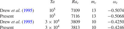
 $m$. The linearized fully compressible equations were spatially discretized using the Chebyshev collocation method (Trefethen Reference Trefethen2000) in the radial direction and spherical harmonic expansion in the angular directions. With a normal mode expansion, a shift-invert preconditioner and the Arnoldi algorithm were employed to solve the resulting eigenvalue problem (Sánchez, Garcia & Net Reference Sánchez, Garcia and Net2016a; Sánchez et al. Reference Sánchez, García and Net2016b). The detailed numerical procedures have been elaborated and validated in our previous work (Liu et al. Reference Liu, Wan, Yan, Sun and Sun2019). To validate our numerical computations, the instability of nearly adiabatic flows (
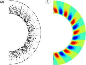
 $n=1.499$) is considered, and we compare the critical parameters based on our fully compressible equations and the result reported by Drew et al. (Reference Drew, Jones and Zhang1995) which is based on the anelastic equations. The comparison of the critical parameters and the critical eigenmodes are shown in table 1 and figure 1, respectively. Our result is in good agreement with Drew et al. (Reference Drew, Jones and Zhang1995), indicating the reliability of our computations.
The comparison of critical parameters based on fully compressible equations for nearly adiabatic flows ( $n=1.499$) and anelastic equations (Drew et al. Reference Drew, Jones and Zhang1995) for
 $(\eta , N_{\rho },Pr)=(0.6,5,1)$. The critical parameters are converted to our dimensionless form with the transformations:
 $Ra = Ra^{D}N_{\rho }(1-\eta )^{2}/(\lambda _{b}n_{a}),m = m^{D}, \omega = \omega ^{D} \sqrt {Pr/Ra}$ (the superscript
 $D$ indicates dimensionless variables employed in Drew et al. Reference Drew, Jones and Zhang1995).

Distribution of  $u_{r}$ of the critical eigenmodes in the equatorial plane for the case with
 $(\eta ,Pr, N_{\rho },Ta)=(0.6,1,5,10^{5})$. (a) Critical eigenmode based on the anelastic equations, (b) critical eigenmode based on the fully compressible equations.

3. Results and discussions
The linear stability analysis for compressible convection in rapidly rotating spherical shells is presented. For an ideal gas, when the specific heat ratio  $\gamma =5/3$, the adiabatic polytropic index is
 $n_{a}=1.5$. The nearly adiabatic base state under thermal and static equilibrium with polytropic index
 $n=1.499$ is considered. The maximum value of density scale height
 $N_{\rho }=\ln (\bar {\rho }_{i}/\bar {\rho }_{o} )$ is
 $5$, which means the density ratio between the inner and outer boundaries is up to 148. In this paper, the radius ratio
 $\eta$ varies from
 $0.2$ to
 $0.6$ in order to explore the influence of the radius ratio on the onset of convection in detail. Moreover, the physical mechanisms for each instability mode will be presented and compared in a quantitative way.
3.1. The influence of the radius ratio on instability processes
The onset of rapidly rotating spherical convection has been wildly studied. The columnar mode was predicted by Roberts (Reference Roberts1968) and Busse (Reference Busse1970), and convective instability in the form of prograde spiralling drifting columnar rolls was found for fluids of moderately small  $Pr$ (Zhang Reference Zhang1992). For small
 $Pr$, the most unstable mode is the inertial mode (Zhang & Busse Reference Zhang and Busse1987; Zhang Reference Zhang1993, Reference Zhang1994). In fully compressible convection with small
 $Pr$ and large
 $N_\rho$, a new instability mode, named the quasi-geostrophic compressible mode, was found in a rapidly rotating spherical shell with
 $\eta =0.4$ (Liu et al. Reference Liu, Wan, Yan, Sun and Sun2019). In a rapidly rotating system, the instability modes have the characteristics of geostrophic balance due to the Taylor–Proudman effect. And the third mode intrinsically depends upon the presence of the time derivative of the density perturbation in the mass conservation equation. So it is called the quasi-geostrophic compressible mode. Thus, in this section, we will study the influence of
 $\eta$ on instability processes, particularly the new instability mode, using the linear stability analysis based on the fully compressible equations in rapidly rotating spherical shells with different
 $\eta$.
We first study the onset of convection for different  $\eta$,
 $Pr$ and
 $N_\rho$. For a fixed
 $\eta$, the instability processes are found to be sensitive to the variations of
 $Pr$ and
 $N_\rho$. However, the leading instability mode still is one of the three types of mode, i.e. the columnar mode, the inertial mode and the quasi-geostrophic compressible mode. Although the radius ratio significantly affects the stability characteristics of the base state for some parameter combinations (
 $N_\rho , Pr$), it should be noted that the quasi-geostrophic compressible mode can be identified at all
 $\eta$.
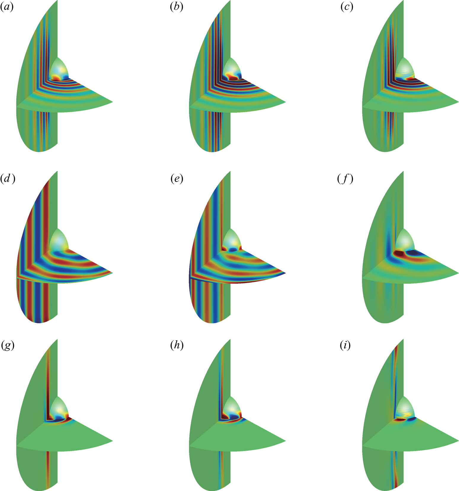
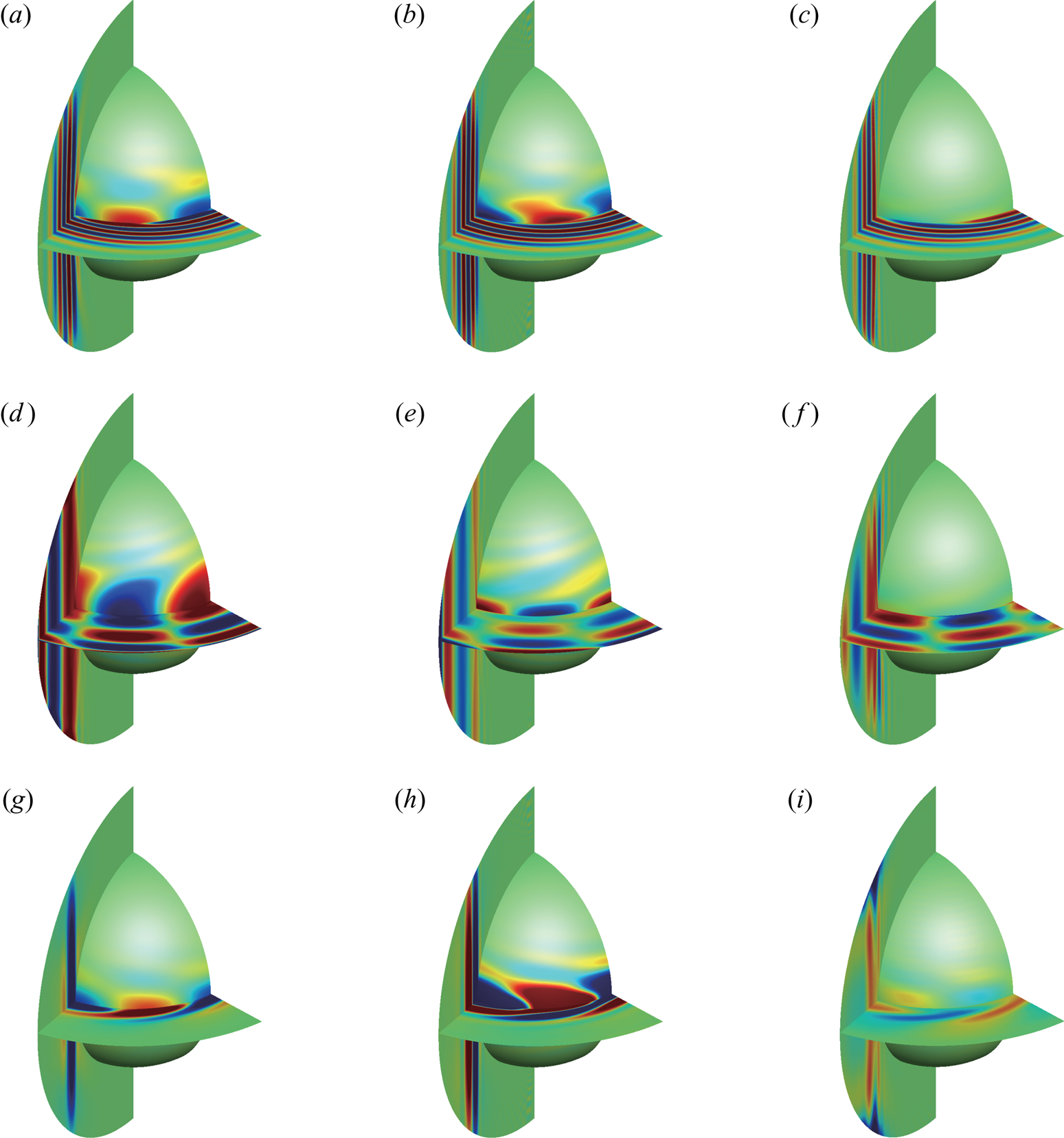
Figures 2 and 3 show the spatial structures of different instability modes for the parameter combination of  $(Ta,m)=(10^{10},5)$ for
 $\eta =0.2$ and
 $\eta =0.6$, respectively. The inertial mode is easy to distinguish because its disturbance occurs near the outer shell, unlike the other two modes. Although the disturbances concentrate in the neighbourhood of the tangent cylinder of the inner core for both the columnar mode and the quasi-geostrophic compressible mode, these two modes can be distinguished according to the critical
 $Ra$. In general, the critical
 $Ra$ is larger than
 $10^{4}$ for columnar modes and it is less than
 $10^{3}$ for the quasi-geostrophic compressible modes. Usually, at a large
 $Pr$, the base state loses stability by the columnar mode with a relatively high critical Rayleigh number
 $Ra_c$.
The spatial structures of different instability modes at  $\eta =0.2$,
 $Ta=10^{10}, m=5$. (a–c) The columnar mode,
 $Pr=0.4$,
 $N_{\rho }=3.0$, the critical Rayleigh number
 $Ra_{c}=8.816\times 10^{5}$, critical frequency
 $\omega _{c}=-1.361$; (d–f) the inertial mode,
 $Pr=0.2$,
 $N_{\rho }=1.0$,
 $Ra_{c}=1.308\times 10^{5}$,
 $\omega _{c}=-4.295$; (g–i) the quasi-geostrophic compressible mode,
 $Pr=0.1$,
 $N_{\rho }=3.0$,
 $Ra_{c}=1.396\times 10^{2}$,
 $\omega _{c}=-42.34$. (a,d,g) The perturbed density
 $\rho '$. (b,e,h) Perturbed azimuthal velocity
 $u_{\phi }^{\prime }$. (c,f,i) The divergence of perturbed velocities
 $\boldsymbol {\nabla } \boldsymbol {\cdot } \boldsymbol {u^{\prime }}$.

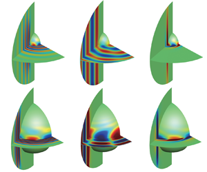
The spatial structures of different instability modes at  $\eta =0.6, Ta=10^{10}, m=5$. (a–c) The columnar mode,
 $Pr=0.4$,
 $N_{\rho }=3.0$, critical Rayleigh number
 $Ra_{c}=2.187\times 10^{7}$, critical frequency
 $\omega _{c}=-0.123$; (d–f) the inertial mode,
 $Pr=0.1$,
 $N_{\rho }=1. 0$,
 $Ra_{c}=1. 543\times 10^{3}$,
 $\omega _{c}=-7.70$; (g–i) the quasi-geostrophic compressible mode,
 $Pr=0.1$,
 $N_{\rho }=3. 0$,
 $Ra_{c}=5. 029\times 10^{2}$,
 $\omega _{c}=-4. 65$. (a,d,g) The perturbed density
 $\rho '$. (b,e,h) Perturbed azimuthal velocity
 $u_{\phi }^{\prime }$. (c,f,i) The divergence of perturbed velocities
 $\boldsymbol {\nabla } \boldsymbol {\cdot } \boldsymbol {u^{\prime }}$.

With  $\eta =0.2$ and
 $(Pr,N_{\rho }) = (0.4,3.0)$, the disturbance is in the form of spiralling drifting columnar rolls, which are aligned with the axis of rotation due to a strong Taylor–Proudman effect, as shown in figure 2(a). The
 $Ra_c$ is approximately
 $8.816\times 10^{5}$. For small
 $Pr$ and a certain intensity of density stratification, the inertial mode becomes unstable first. Figure 2(b) shows the spatial structures of the inertial mode with
 $(Pr,N_{\rho }) = (0.1,1.0)$ with strong disturbances located in the equatorial region. With small
 $Pr$ and large
 $N_{\rho }$, the quasi-geostrophic compressible mode occurs, and its spatial structures are shown in figure 2(c). We find that the disturbances concentrate in the neighbourhood of the tangent cylinder of the inner core, and evident quasi-geostrophic characteristics can also be found. However, although both the columnar mode and the quasi-geostrophic compressible mode exhibit quasi-geostrophic characteristics, their critical Rayleigh numbers are different by several orders of magnitude. For the columnar mode, the divergence of velocities almost does not change along with the columnar rolls except near the boundary. In contrast, the divergence of velocities changes sign where the convection rolls intersect the outer sphere for the quasi-geostrophic compressible mode. The typical instability modes in a spherical shell with
 $\eta =0.6$ are also shown in figure 3 for
 $Ta=10^{10}$ and
 $m=5$. By comparing figures 2 and 3, it is easy to find that the structures of the same mode for different
 $\eta$ are quite similar. However, the parameter space in which these modes dominate the instability is substantially affected by
 $\eta$.
Here, we present the influence of  $\eta$ on the instability processes in the parameter space of (
 $N_{\rho }, Pr$). The Prandtl number varies from 0.1 to 0.8, and both weak and strong density stratification cases are considered with
 $0.01 \leqslant N_{\rho } \leqslant 5$. Since the instability processes are rather complicated, including different mode switchings in a broad range of (
 $N_{\rho }, Pr$), for clarity, Liu et al. (Reference Liu, Wan, Yan, Sun and Sun2019) approximately classified the instability processes into five categories, according to the variation of the maximal growth rate
 $\sigma$ with
 $Ra$ and the dominant instability mode. In the following, we briefly introduce the five categories:
(i) With small
 $N_{\rho }$ and large $Pr$, the columnar mode loses stability first as $Ra$ increases, and the $Ra_c$ is relatively high.
(ii) With increasing
$N_\rho$, the quasi-geostrophic compressible mode appears first at a relatively large $Pr$, and the $Ra_c$ is relatively low. With increasing $Ra$, this mode gains stability again, while the columnar mode occurs at a relatively high $Ra$. This means the base state undergoes the ‘stable $\to$ unstable $\to$ stable $\to$ unstable’ process.(iii) With small
$Pr$ and a certain $N_\rho$, the inertial mode loses stability as $Ra$ increases. The base state undergoes the ‘stable $\to$ unstable’ process.(iv) At small
$Pr$ and moderate $N_\rho$, the base state becomes unstable by the quasi-geostrophic compressible mode first, which becomes stable with increasing $Ra$. As $Ra$ increases further, the inertial mode finally loses stability and dominates the flow. This also means the base state undergoes the ‘stable $\to$ unstable $\to$ stable $\to$ unstable’ process.(v) With small
$Pr$ and large $N_\rho$, the base state loses stability at a relatively low $Ra$ due to the quasi-geostrophic compressible mode and keeps being unstable at higher $Ra$.


It should be noted that there are other more complex instability processes indicated by the black crosses in the phase diagrams in addition to the above five instability processes, in which the base state undergoes the process of ‘stable  $\to$ unstable
 $\to$ stable’ many times due to mode switching and eventually becomes unstable.
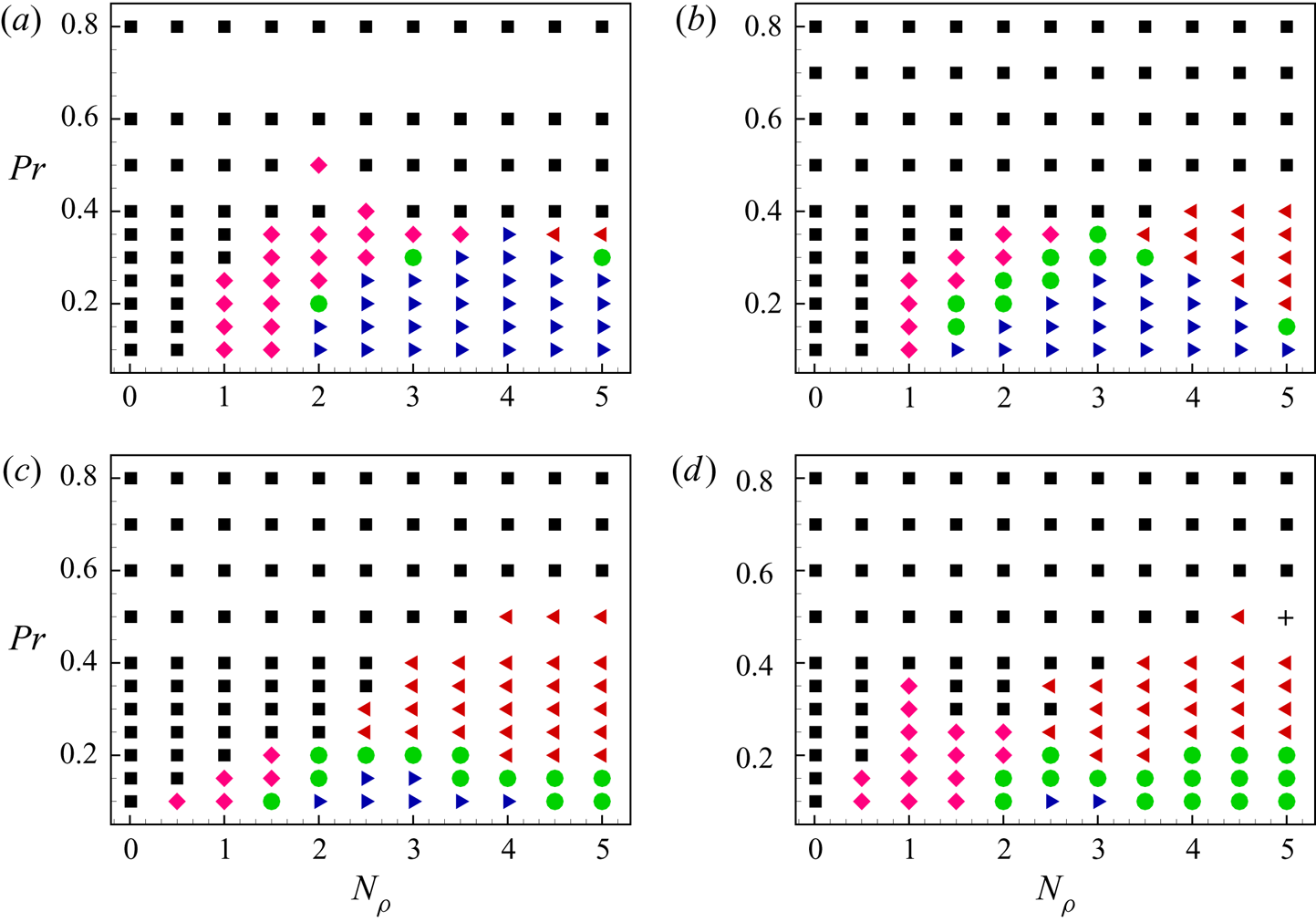
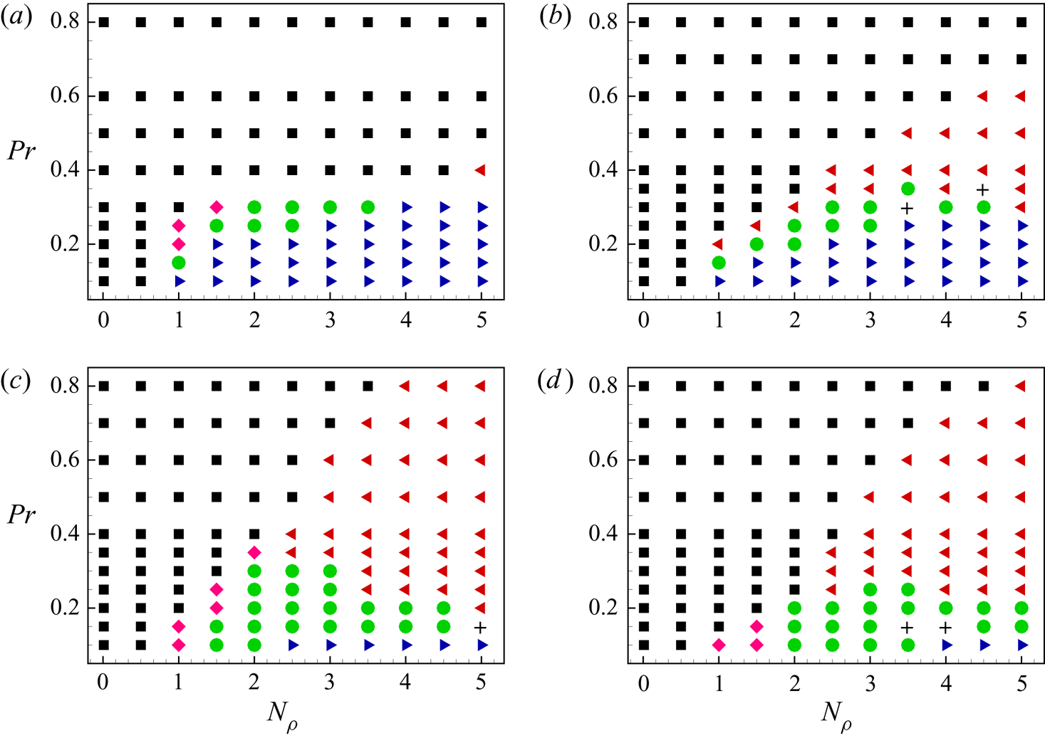
In order to compare with the results in Liu et al. (Reference Liu, Wan, Yan, Sun and Sun2019), four more different radius ratios  $\eta =0.2,0.3,0.5,0.6$ are considered. The phase diagrams of instability processes that are represented by the above five categories in the parameter space of (
 $N_{\rho }, Pr$) are given in figure 4 for
 $(Ta,m)=(10^{8},5)$ and in figure 5 for
 $(Ta,m)=(10^{10},10)$, respectively. For both parameter combinations of
 $(Ta,m)$, the phase diagrams at different
 $\eta$ have certain similarities in terms of the appearance of different types of instability processes. However, in the phase diagram,
 $\eta$ has a great influence quantitatively on the parameter space of various modes.
The phase diagrams at different radius ratios of instability processes in the parameter space of  $(N_{\rho }, Pr)$ for specified wavenumber
 $m=5$ and specified Taylor number
 $Ta=10^{8}$ at (a)
 $\eta =0.2$, (b)
 $\eta =0.3$, (c)
 $\eta =0.5$, (d)
 $\eta =0.6$. Five instability processes are represented by the symbols black squares
 $\blacksquare$ (I), red left-pointing triangles
 $\blacktriangleleft$ (II), purple rhombi
 $\blacklozenge$ (III), green circles
 $\bullet$ (IV) and blue right-pointing triangles
 $\blacktriangleright$ (V), respectively. The symbols black crosses
 ${\pmb {+}}$ in (d) represent the more complex instability processes in the present parameter space.

The phase diagrams at different radius ratios of instability processes in the parameter space of  $(N_{\rho }, Pr)$ for specified wavenumber
 $m=10$ and specified Taylor number
 $Ta=10^{10}$ at (a)
 $\eta =0.2$, (b)
 $\eta =0.3$, (c)
 $\eta =0.5$, (d)
 $\eta =0.6$. Five instability processes are represented by the symbols black squares
 $\blacksquare$ (I), red left-pointing triangles
 $\blacktriangleleft$ (II), purple rhombi
 $\blacklozenge$ (III), green circles
 $\bullet$ (IV) and blue right-pointing triangles
 $\blacktriangleright$ (V), respectively. The symbols black crosses
 ${\pmb {+}}$ represent the more complex instability processes in the present parameter space.

In figure 4 for  $Ta=10^{8}$, category I occurs in the top and bottom left of the phase diagram for all
 $\eta$, suggesting that, at large
 $Pr$, the columnar mode is still the most important even with strong compressibility, and this kind of onset behaviour seems to be insensitive to
 $\eta$. However, with
 $Pr$ declining or
 $N_{\rho }$ increasing, instability processes for convection onset become more complex, and are sensitive to
 $\eta$ change. Category II occurs in the middle right of the phase diagram and the extent of the parameter space increases obviously with the increase of
 $\eta$. Category III occurs at small
 $Pr$ and certain
 $N_{\rho }$ and the influence of
 $\eta$ on this category is rather complicated. For small
 $\eta$, category IV occurs at medium
 $N_{\rho }$ and
 $Pr$. However, as
 $\eta$ increases, the parameter space of (
 $N_{\rho }, Pr$) for category IV expands slightly and moves to small
 $Pr$ and large
 $N_{\rho }$. With small
 $Pr$ and large
 $N_{\rho }$, the base state loses stability by category V, and this kind of behaviour is strongly influenced by
 $\eta$. As
 $\eta$ increases, the parameter space of (
 $N_{\rho }, Pr$) for category V is reduced and this instability process only occurs at very small
 $Pr$ for large
 $\eta$.
In the phase diagrams in figure 5, there are some details that are different from those for  $Ta=10^{8}$ in figure 4. For large
 $\eta$, category II occurs at the parameter space of large
 $N_{\rho }$ and large
 $Pr$, where the instability process belongs to the category I for
 $Ta=10^{8}$ in figure 4. Besides, it can be found that the parameter space for category III is reduced for all
 $\eta$ compared with figure 4. It should be also noted that the phase diagrams have certain similarities for all
 $\eta$. As
 $\eta$ increases, the parameter space for category II expands and parameter space for category V shrinks, which is the same as figure 4.
3.2. The influence of $\eta$ on critical parameters

In this section, the instability of the base state to general disturbances is studied. As previously mentioned, the instability process of the base state is complex at some parameter combinations for a specific  $m$. Here, we first define the critical parameter
 $Ra_{c,m}$ as the lowest
 $Ra$ of convection onset for a specified
 $m$, leaving out possible ‘stable
 $\to$ unstable’ and ‘unstable
 $\to$ stable’ processes at higher
 $Ra$. Then, the critical Rayleigh number
 $Ra_{c}$ for general disturbances is defined as the smallest
 $Ra_{c,m}$ with respect to different wavenumbers
 $m$, i.e.
 $Ra_c= \min _m Ra_{c,m}$. The critical wavenumber
 $m_{c}$ is obtained corresponding to the specific
 $Ra_c$.
For large Taylor numbers,  $Ta \geqslant 10^{7}$, the scaling behaviour of
 $Ra_{c}$ with
 $Ta$ was found by Calkins et al. (Reference Calkins, Julien and Marti2015b). Liu et al. (Reference Liu, Wan, Yan, Sun and Sun2019) also found that the
 $Ra_{c}$ and
 $m_{c}$ follow very similar scaling laws with
 $Ta$ for two different modes, i.e. the quasi-geostrophic compressible mode and columnar mode, at
 $\eta = 0.4$. Here, the influence of
 $\eta$ on the scaling behaviour of
 $Ra_c$ is further investigated. As shown in figures 4 and 5, for all
 $\eta$, a general trend is that the columnar mode becomes unstable first at large
 $Pr$ and the quasi-geostrophic compressible mode becomes unstable first at very small
 $Pr$. Therefore, for clarity, we only consider the smallest and largest radius ratios, i.e.
 $\eta =0.2$,
 $0.6$ and the largest and smallest Prandtl numbers,
 $Pr=1$,
 $0.1$, and then the relationship between critical parameters (
 $Ra_{c},m_{c}$) and
 $Ta$ is presented.
Firstly, the critical parameters at  $Pr=1$ are studied for
 $\eta =0.2$,
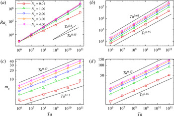
 $0.6$. Figure 6 shows
 $Ra_c$ and
 $m_{c}$ as functions of
 $Ta$ for different
 $N_{\rho }$. In these cases, the instability is dominated by the columnar mode. By comparing the critical parameters of different
 $\eta$, we find that the change trends of
 $Ra_{c}$ and
 $m_{c}$ with
 $Ta$ at two different
 $\eta$ are quite similar. It is seen that
 $Ra_{c}$ and
 $m_{c}$ increase as
 $N_{\rho }$ increases. The
 $Ra_c$ increases as
 $Ta$ increases, implying that the stronger Taylor–Proudman effect suppresses the occurrence of convection. Besides, the
 $Ra_c$ satisfies certain scaling laws with
 $Ta$, and the scaling exponents are approximately 0.6 for most
 $N_\rho$. Similarly,
 $m_{c}$ also increases as
 $Ta$ increases, and satisfies certain scaling laws with
 $Ta$. However, some differences between the two different
 $\eta$ can also be identified. For
 $\eta =0.2$, the density stratification has little effect on
 $Ra_c$, while for
 $\eta =0.6$, the
 $Ra_c$ increases with increasing
 $N_\rho$. For
 $\eta =0.6$, the scaling exponents for
 $Ra_{c}$ and
 $m_{c}$ vary little with
 $N_{\rho }$, which is consistent with the results of
 $\eta =0.4$ (Liu et al. Reference Liu, Wan, Yan, Sun and Sun2019). The scaling exponent of
 $Ra_c$ for
 $N_{\rho }=0.01$ decreases to
 $0.45$ at
 $\eta =0.2$. Furthermore, it is noted that
 $Ra_c$ and
 $m_c$ at
 $\eta =0.6$ are much larger than those at
 $\eta =0.2$.
(a,b) The critical Rayleigh numbers  $Ra_{c}$ (a,b) and the critical wavenumbers
 $m_{c}$ (c,d) as functions of
 $Ta$ at
 $Pr=1.0$ for different
 $N_{\rho }$ at (a,c)
 $\eta =0.2$ and (b,d)
 $\eta =0.6$.

Next, we study the critical parameters at  $Pr=0.1$ for
 $\eta =0.2$ and
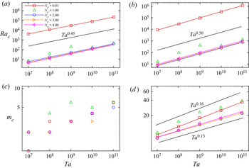
 $0.6$. Figure 7 shows
 $Ra_c$ and
 $m_c$ as functions of
 $Ta$ for different
 $N_{\rho }$. For this small
 $Pr$, the dominant mode is the columnar mode only for small density stratification (
 $N_{\rho }=0.01$). For large
 $N_{\rho }$ (
 $N_{\rho } \geqslant 2.0$), the instability is dominated by the quasi-geostrophic compressible mode. However, for
 $N_{\rho }=1$, the inertial mode sometimes becomes the dominant mode. There are two dominated modes for
 $N_{\rho }=1.0$, so the
 $m_{c}$ does not increase monotonically with increasing
 $Ta$ in figure 7(c). Besides, the scaling laws of critical
 $Ra_{c}$ and
 $Ta$ are failed when
 $N_{\rho }=1.0$ as figure 7(a,b) show. Except this special case,
 $Ra_{c}$ increases as
 $Ta$ increases and satisfies certain scaling laws with
 $Ta$ for the same instability mode. Besides, it is seen that the scaling exponents of the columnar mode and quasi-geostrophic compressible mode are very close, even though the corresponding
 $Ra_c$ are quite different. For the quasi-geostrophic compressible mode, the density stratification parameter
 $N_\rho$ has little effect on
 $Ra_c$. For
 $\eta =0.6$,
 $m_{c}$ satisfies certain scaling laws with
 $Ta$ for the same mode, but these scaling laws have not been found for
 $\eta =0.2$, which might be attributed to the very small values of
 $m_{c}$. Moreover, it is also seen that the critical parameters
 $Ra_c$ and
 $m_c$ at
 $\eta =0.6$ are much larger than those at
 $\eta =0.2$, similar to the results at
 $Pr=1$.
(a,b) The critical Rayleigh numbers  $Ra_{c}$ (a,b) and the critical wavenumbers
 $m_{c}$ (c,d) as functions of
 $Ta$ at
 $Pr=0.1$ for different
 $N_{\rho }$ at (a,c)
 $\eta =0.2$ and (b,d)
 $\eta =0.6$.

Finally, as mentioned above, there is a considerable difference between the critical parameters for  $\eta =0.2$,
 $0.6$. Therefore, the influence of
 $\eta$ on the critical parameters is investigated in detail. We calculate the
 $Ra_{c}$ and
 $m_{c}$ for different radius ratios (
 $0.2 \leqslant \eta \leqslant 0.6$) at fixed
 $Ta$ and
 $Pr$. Figures 8 and figure 9 show the influence of
 $\eta$ on the critical parameters at four parameter combinations
 $(Ta, Pr)=(10^{8}, 1.0)$,
 $(10^{8}, 0.1)$,
 $(10^{10},1.0)$,
 $(10^{10},0.1)$. At
 $Pr=1.0$, as shown in figure 8(a,c), the
 $Ra_{c}$ increases as
 $\eta$ increases. In this case, the base state loses stability by the columnar mode. We can also find that the
 $Ra_c$ becomes larger at a larger
 $N_\rho$. At
 $Pr=0.1$, the quasi-geostrophic compressible mode is usually the most unstable mode for large
 $N_\rho$. As shown in figure 8(b,d), the change trend of
 $Ra_{c}$ with
 $\eta$ is similar to that at
 $Pr=1.0$, i.e. the
 $Ra_c$ increases with
 $\eta$. However, different from the columnar mode, the effect of
 $N_\rho$ on
 $Ra_{c}$ becomes much smaller for the quasi-geostrophic compressible mode. In figure 9(a,c), it is further found that the
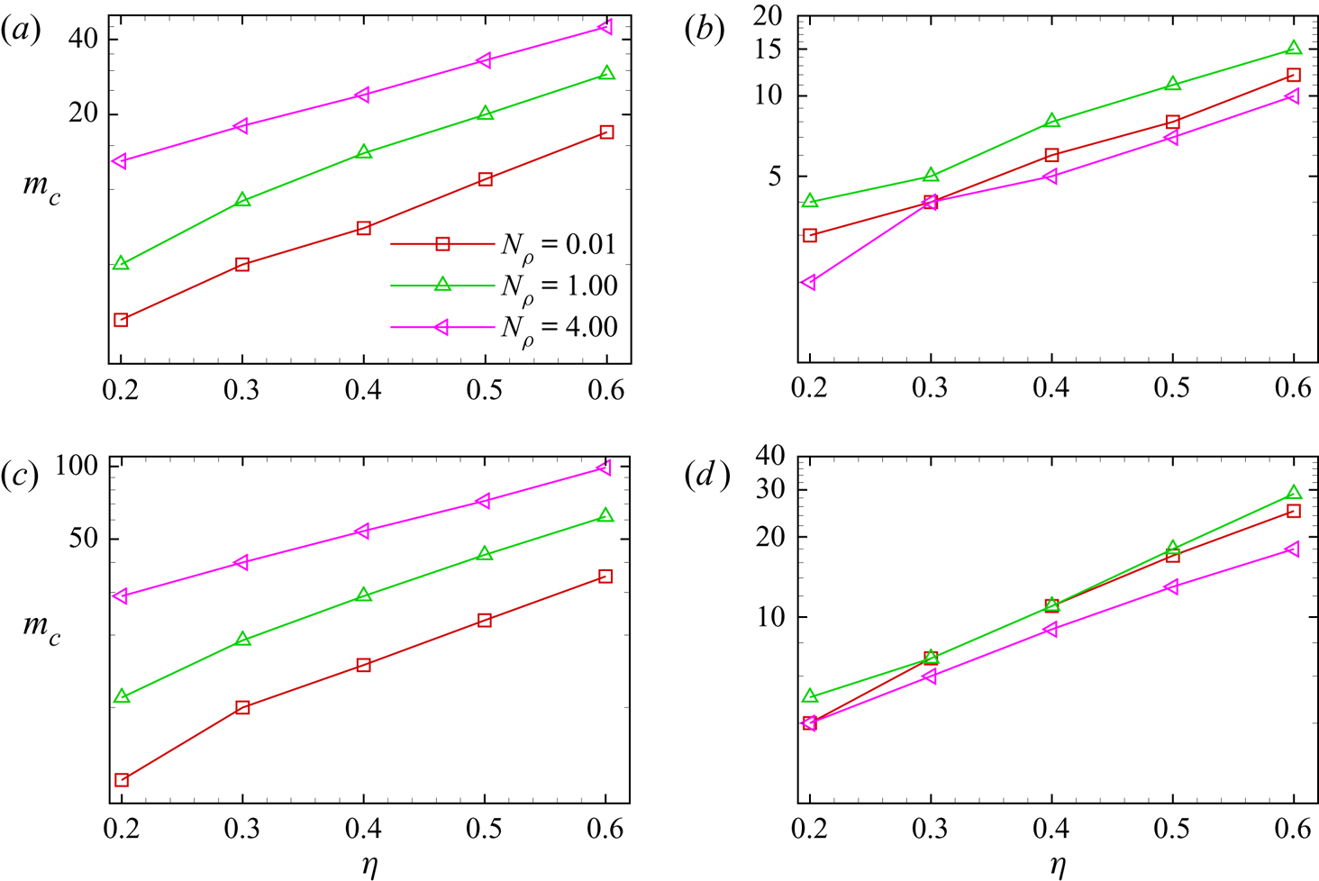
 $m_c$ increases with
 $\eta$ for
 $Pr=1.0$. The larger
 $N_\rho$ is, the larger
 $m_c$ is. In figure 9(b,d),
 $m_c$ also increases with
 $\eta$ for
 $Pr=0.1$, but the differences in
 $m_c$ for different
 $N_\rho$ become much smaller.
Critical Rayleigh numbers  $Ra_{c}$ as functions of
 $\eta$ for different
 $N_{\rho }$ at (a)
 $Ta=10^{8},Pr=1.0$; (b)
 $Ta=10^{8}, Pr=0.1$; (c)
 $Ta=10^{10},Pr=1.0$; (d)
 $Ta=10^{10},Pr=0.1$.

Critical wavenumbers  $m_{c}$ as functions of
 $\eta$ for different
 $N_{\rho }$ at (a)
 $Ta=10^{8},Pr=1.0$; (b)
 $Ta=10^{8}, Pr=0.1$; (c)
 $Ta=10^{10},Pr=1.0$; (d)
 $Ta=10^{10},Pr=0.1$.

In short, we illustrate that  $\eta$ has a significant influence on
 $Ra_c$ and
 $m_c$, which increase with
 $\eta$ for both the columnar mode and the quasi-geostrophic compressible mode. The increase of
 $\eta$ always tends to stabilize the flow to some extent.
3.3. Analysis based on linearized perturbation equations
As previously mentioned, there are very similar characteristics between the columnar mode and the quasi-geostrophic compressible mode, as illustrated in figure 2. However, their critical Rayleigh numbers are different by several orders of magnitude, and the two modes occur in different parameter spaces (see figure 4), implying that two modes are driven by different physical mechanisms. To gain more physical insights into the two instability modes, the balance of the linearized perturbation equations, as well as the influence of  $\eta$, are considered in this section. It is well known that, in a rapidly rotating system, the physical quantity usually varies weakly with the axis of rotation due to the strong Taylor–Proudman effect. For the sake of analysis, a cylindrical coordinate system
 $(R,\phi ,z)$ with the centre of the sphere as the origin is established, where
 $R$ is the distance to the axis of rotation,
 $\phi$ is the azimuthal angle and
 $z$ is the axial location along the axis of rotation.
Here, we mainly concern with the statistics of each term in the linearized perturbation equations. For convenience, we use a set of variables  $\mathcal {F}_{1\sim 3}$ to represent the terms in the continuity equation (2.8a)
 \begin{equation} \mathcal{F}_{1}=\frac{\partial \rho^{\prime} }{\partial t}, \qquad \mathcal{F}_{2}=\boldsymbol{\nabla} \bar{\rho} \boldsymbol{\cdot} \boldsymbol{u}^{\prime}, \quad \mathcal{F}_{3}=\bar{\rho} \boldsymbol{\nabla} \boldsymbol{\cdot} \boldsymbol{u}^{\prime}.\quad \end{equation}
The terms in the radial component of the momentum equation (2.8b) are represented by  $\mathcal {F}_{4\sim 9}$
 \begin{equation} \left.\begin{gathered}
\mathcal{F}_{4}=\bar{\rho} \frac{\partial
\boldsymbol{u}^{\prime}}{\partial t} \boldsymbol{\cdot} \hat{r}, \quad
\mathcal{F}_{5}=\sqrt{\frac{P r T a}{R a}} \bar{\rho}\!\left(\hat{z} \times \boldsymbol{u}^{\prime}\right) \boldsymbol{\cdot} \hat{r}, \quad
\mathcal{F}_{6}=\frac{\nabla p^{\prime} \boldsymbol{\cdot} \hat{r}}{\epsilon}, \\
\mathcal{F}_{7}=\sqrt{\frac{P r}{R a}}
\left(\nabla^{2}\boldsymbol{u}^{\prime}\right) \boldsymbol{\cdot} \hat{r},\quad
\mathcal{F}_{8}=\frac{\rho^{\prime} }{\epsilon(1-\eta)^{2} r^{2}}, \quad
\mathcal{F}_{9}=\frac{1}{3}\sqrt{\frac{P r}{R a}}
\left(\nabla\!\left(\boldsymbol{\nabla} \boldsymbol{\cdot}
\boldsymbol{u}^{\prime}\right)\right)\boldsymbol{\cdot} \hat{r},
\end{gathered}\right\}
\end{equation}
and the terms in the energy equation (2.8c) are represented by  $\mathcal {F}_{10\sim 13}$
 \begin{align} \mathcal{F}_{10}=\bar{\rho} \frac{\partial T^{\prime}}{\partial t}, \quad \mathcal{F}_{11}=\bar{\rho}\boldsymbol{u}^{\prime} \boldsymbol{\cdot} \boldsymbol{\nabla} \bar{T}, \quad \mathcal{F}_{12}= (\gamma-1) \bar{p} \boldsymbol{\nabla} \boldsymbol{\cdot} \boldsymbol{u}^{\prime}, \quad \mathcal{F}_{13}=\frac{\gamma}{\sqrt{Pr Ra}} \nabla ^{2} T^{\prime}. \end{align}
For the three dominant instability modes, we studied the relative magnitudes of all variables  $\mathcal {F}_{i=1\sim 13}$ as functions of
 $R$. By taking the average of
 $\mathcal {F}_{i}^{2}$ in the
 $\phi$ and
 $z$ directions and calculating the square root, we can get the radial profiles of the surface averaged value
 $\left \langle \mathcal {F}_{i}\right \rangle ^{S}_{R}$
 \begin{equation} \left\langle\mathcal{F}_{i} \right\rangle_R^{S} =\left(\int_{0}^{2{\rm \pi}}\int_{z}\mathcal{F}_{i}^{2}R \,\textrm{d}z\,\textrm{d}\phi \right)^{1/2}\left(\int_{0}^{2{\rm \pi}}\int_{z}R \,\textrm{d}z \,\textrm{d}\phi\right)^{{-}1/2}. \end{equation}
Then,  $\left \langle \mathcal {F}_{i}\right \rangle ^{S}_{R}$ is further normalized by the maximum value of
 $\left \langle \mathcal {F}_{i}^{S}\right \rangle _{R}$ for all values of
 $R$ in the same equation
 $$\begin{gather} \left\langle F_{i}\right\rangle_R = \frac{\left\langle \mathcal{F}_{i}\right\rangle _{R}^{S}}{\max\left\{ \left\langle \mathcal{F}_{1}\right\rangle _{R}^{S}, \left\langle \mathcal{F}_{2}\right\rangle _{R}^{S}, \left\langle \mathcal{F}_{3}\right\rangle _{R}^{S} \right\}} , \quad i=1\sim 3; \end{gather}$$
 $$\begin{gather}\left\langle F_{i}\right\rangle _R = \frac{\left\langle \mathcal{F}_{i}\right\rangle _{R}^{S}}{\max\left\{ \left\langle \mathcal{F}_{4}\right\rangle _{R}^{S}, \left\langle \mathcal{F}_{5}\right\rangle _{R}^{S}, \ldots \left\langle \mathcal{F}_{9}\right\rangle _{R}^{S} \right\}} ,\quad i=4 \sim 9; \end{gather}$$
 $$\begin{gather}\left\langle F_{i}\right\rangle _R = \frac{\left\langle \mathcal{F}_{i}\right\rangle _{R}^{S}}{\max\left\{ \left\langle \mathcal{F}_{10}\right\rangle _{R}^{S}, \ldots \left\langle \mathcal{F}_{13}\right\rangle _{R}^{S} \right\}} , \quad i=10\sim 13. \end{gather}$$
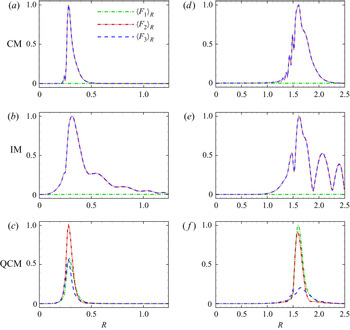
Figure 10 shows  $\left \langle F_{1\sim 3}\right \rangle _{R}$ in the perturbed continuity equation for the three instability modes with
 $\eta =0.2$ and
 $0.6$. By comparing the relative magnitude of each term for different modes, we find that the term
 $\left \langle F_1 \right \rangle _{R}$ plays a very important role in the quasi-geostrophic compressible mode which is negligibly small for all positions in the columnar mode and inertial mode. For the quasi-geostrophic compressible mode, the time derivative term of disturbance density is as important as the other two terms. The magnitude of
 $\left \langle F_1\right \rangle _{R}$ is comparable to that of
 $\left \langle F_3 \right \rangle _{R}$ in the case with
 $\eta =0.2$. Similarly, with
 $\eta =0.6$, its magnitude is in general comparable to that of the term
 $\left \langle F_2 \right \rangle _{R}$. This clearly implies that the classical anelastic model is unable to capture the quasi-geostrophic compressible mode.
The radial profiles of  $\left \langle F_{i}\right \rangle _{R}$ in the continuity equation for different instability modes at
 $Ta=10^{10},m=5$ for
 $\eta =0.2$ and
 $\eta =0.6$: (a,d)
 $Pr=0.8, N_{\rho }=3. 0$, the columnar mode (CM); (b)
 $Pr=0.2, N_{\rho }=1. 0$; (e)
 $Pr=0.1, N_{\rho }=1. 0$, the inertial mode (IM); (c,f)
 $Pr=0.1, N_{\rho }=3. 0$, the quasi-geostrophic compressible mode (QCM). Panels (a–c)
 $\eta =0.2$, (d–f)
 $\eta =0.6$. The value of
 $Ra_{c}$ for each case: (a)
 $1.300\times 10^{6}$; (b)
 $1.308\times 10^{5}$; (c)
 $1.397\times 10^{2}$; (d)
 $3.243\times 10^{7}$; (e)
 $1.451\times 10^{6}$; (f)
 $5.023\times 10^{2}$.

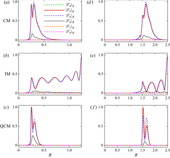
Figure 11 shows  $\left \langle F_{4\sim 9}\right \rangle _{R}$ corresponding to the terms in the perturbed radial momentum equation for the three instability eigenmodes as functions of
 $R$ at
 $Ta=10^{10}$. For all the instability modes, the three leading terms are the Coriolis force term
 $\left \langle F_{5}\right \rangle _{R}$, pressure gradient term
 $\left \langle F_{6}\right \rangle _{R}$ and buoyancy term
 $\left \langle F_{8}\right \rangle _{R}$, while the other terms are very small. In terms of amplitude, the buoyancy term
 $\left \langle F_{8}\right \rangle _{R}$ is much smaller than the terms
 $\left \langle F_{5}\right \rangle _{R}$ and
 $\left \langle F_{6}\right \rangle _{R}$, although it seems to be a little bit more important in the quasi-geostrophic compressible mode, as illustrated in figure 11(c). In general, the radial momentum equation is mainly governed by the actions of the Coriolis force and pressure gradient for all modes due to rapid rotations.
The  $\left \langle F_{i}\right \rangle _{R}$ in the radial momentum equation for different instability eigenmodes as functions of the distance to the axis of rotation
 $R$ at
 $Ta=10^{10},m=5$: (a,d)
 $Pr=0.8, N_{\rho }=3. 0$, the columnar mode; (b)
 $Pr=0.2, N_{\rho }=1. 0$, (e)
 $Pr=0.1, N_{\rho }=1. 0$, the inertial mode; (c,f)
 $Pr=0.1, N_{\rho }=3. 0$, the quasi-geostrophic compressible mode. Panels (a–c)
 $\eta =0.2$, (d–f)
 $\eta =0.6$. Value of
 $Ra_{c}$ for each case: (a)
 $1.300\times 10^{6}$; (b)
 $1.308\times 10^{5}$; (c)
 $1.397\times 10^{2}$; (d)
 $3.243\times 10^{7}$; (e)
 $1.451\times 10^{6}$; (f)
 $5.023\times 10^{2}$.

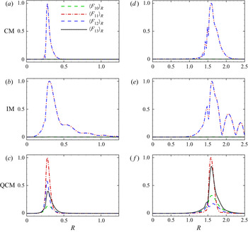
Figure 12 shows  $\left \langle F_{10\sim 13}\right \rangle _{R}$ corresponding to the terms in the perturbed energy equation for three instability eigenmodes as functions of
 $R$ at
 $Ta=10^{10}$. In the columnar mode and inertial mode, the two dominant terms are
 $\left \langle F_{11}\right \rangle _{R}$ and
 $\left \langle F_{12}\right \rangle _{R}$ in terms of magnitude, and the time-derivative term of disturbance temperature
 $\left \langle F_{10}\right \rangle _{R}$ and the disturbance temperature diffusion term
 $\left \langle F_{13}\right \rangle _{R}$ are small enough to be ignored, as illustrated in figure 12(a,b). However, in the quasi-geostrophic compressible mode, the
 $\left \langle F_{13}\right \rangle _{R}$ plays a significant role. As shown in figure 12(c,f), the magnitude of
 $\left \langle F_{13}\right \rangle _{R}$ is comparable to that of
 $\left \langle F_{12}\right \rangle _{R}$ at
 $\eta =0.2$, while it is even close to the leading term
 $\left \langle F_{11}\right \rangle _{R}$ at
 $\eta =0.6$.
The  $\left \langle F_{i}\right \rangle _{R}$ in the energy equation for different instability eigenmodes as functions of the distance to the axis of rotation
 $R$ at
 $Ta=10^{10}$,
 $m=5$: (a,d)
 $Pr=0.8, N_{\rho }=3. 0$, the columnar mode; (b)
 $Pr=0.2, N_{\rho }=1. 0$; (e)
 $Pr=0.1, N_{\rho }=1. 0$, the inertial mode; (c,f)
 $Pr=0.1, N_{\rho }=3. 0$, the quasi-geostrophic compressible mode. Panels (a–c)
 $\eta =0.2$, (d–f)
 $\eta =0.6$. CM: columnar mode; IM: inertial mode; QCM: quasi-geostrophic compressible mode. Value of
 $Ra_{c}$ for each case: (a)
 $1.300\times 10^{6}$; (b)
 $1.308\times 10^{5}$; (c)
 $1.397\times 10^{2}$; (d)
 $3.243\times 10^{7}$; (e)
 $1.451\times 10^{6}$; (f)
 $5.023\times 10^{2}$.

In summary, we find two important terms that should be responsible for the occurrence of the quasi-geostrophic compressible mode, i.e. the time-derivative term of disturbance density  $\mathcal {F}_1$ in the perturbed continuity equation and the disturbance temperature diffusion term
 $\mathcal {F}_{13}$ in the perturbed energy equation. Figure 13 shows the spatial distributions of normalized
 $\mathcal {F}_1$ and
 $\mathcal {F}_{13}$ for different modes at
 $\eta =0.6$ and
 $Ta=10^{10}$. In the columnar mode and inertial mode, their magnitudes in the whole domain are quite small. However, in the quasi-geostrophic compressible mode, they have comparable magnitudes to the leading term of the perturbed equation and exhibit the quasi-geostrophic features. Similar to the spatial distribution of disturbance in figure 2, they are also mainly concentrated in the neighbourhood of the tangent cylinder of the inner core.
The distribution of  ${\partial \rho ^{\prime }}/{\partial t}$ (
 $\mathcal {F}_1$) and
 $({\gamma }/{\sqrt {RaPr}})\nabla ^{2}T^{\prime }$ (
 $\mathcal {F}_{13}$) normalized by the maximum values of
 $\boldsymbol {\nabla } \bar {\rho } \boldsymbol {\cdot } \boldsymbol {u}^{\prime }$ and
 $\bar {\rho }\boldsymbol {u}^{\prime } \boldsymbol {\cdot } \boldsymbol {\nabla } \bar {T}$ for the critical eigenmodes at
 $Ta=10^{10}, \eta =0.6,m=5$: (a,d)
 $Pr=0.8, N_{\rho }=3. 0$, the columnar mode; (b,e)
 $Pr=0.1, N_{\rho }=1. 0$, the inertial mode; (c,f)
 $Pr=0.1, N_{\rho }=3.0$, the quasi-geostrophic compressible mode.

Next, to quantify the influence of  $\eta$ on the instability modes to a certain degree, the relative magnitude of each term
 $\mathcal {F}_{i}$ in the perturbed equations (2.8) for different modes is studied. Here, we calculated the root mean square (rms) of each term
 $\mathcal {F}_{i}$ over the whole space
 $V$
 \begin{equation} {\left\langle {{{\mathcal{F}}_i}} \right\rangle _{rms}^{V}} = \sqrt {\frac{1}{V }\int_V {{\mathcal{F}}_i^{2}} \,\textrm{d}V }. \end{equation}
The relative magnitudes of  $\left \langle \mathcal {F}_{i}\right \rangle _{rms}$ are mainly concerned, so
 $\left \langle \mathcal {F}_{i}\right \rangle _{rms}$ in the continuity and energy equations are normalized as follows:
 $$\begin{gather} \left\langle F_{i}\right\rangle _{rms} = \left\langle \mathcal{F}_{i}\right\rangle _{rms}^{V}/\left\langle \mathcal{F}_{2}\right\rangle _{rms}^{V} , \quad i=1\sim 3; \end{gather}$$
 $$\begin{gather}\left\langle F_{i}\right\rangle _{rms} = \left\langle \mathcal{F}_{i}\right\rangle _{rms}^{V}/\left\langle \mathcal{F}_{11}\right\rangle _{rms}^{V} ,\quad i=10\sim 13. \end{gather}$$
Figure 14 shows  $\left \langle F_{i}\right \rangle _{rms}$ in the continuity and energy equations for
 $Ta=10^{10}, m=5$ and different instability modes. For the columnar mode and inertial mode, the relative magnitudes of terms
 $\left \langle F_{1\sim 3}\right \rangle _{rms}$ and
 $\left \langle F_{10\sim 13}\right \rangle _{rms}$ vary little with
 $\eta$. However, in the quasi-geostrophic compressible mode, we find the relative magnitudes show a strong radius ratio dependency. In the perturbed continuity equation,
 $\left \langle F_{1}\right \rangle _{rms}$ is increased with
 $\eta$. Similarly,
 $\left \langle F_{13}\right \rangle _{rms}$ is also increased with
 $\eta$ in the perturbed energy equation. This implies that, in the system with a larger radius ratio, it may be harder to find the unstable quasi-geostrophic compressible mode over a wide range of
 $Ra$ since it requires higher intensities of
 $\mathcal {F}_{1}$ and
 $\mathcal {F}_{13}$, as shown in the phase diagrams (see figure 4).
The root-mean-square of terms  $\left \langle F_{i}\right \rangle _{rms}$ in the continuity equation normalized by
 $\left \langle \mathcal {F}_{2}\right \rangle _{rms}^{V}$ and in the perturbed energy equation normalized by
 $\left \langle \mathcal {F}_{11}\right \rangle _{rms}^{V}$ for
 $Ta=10^{10}, m=5$. CM: columnar mode (
 $Pr=0.8,N_{\rho }=3.0$); IM: inertial mode (
 $Pr=0.1,N_{\rho }=1.0$); QCM: quasi-geostrophic compressible mode (
 $Pr=0.1,N_{\rho }=3.0$).

3.4. The budget of kinetic energy and flow instability mechanism
To better understand the physical mechanism of the instability mode, the analysis of kinetic energy transport is usually performed (Wanschura, Kuhlmann & Rath Reference Wanschura, Kuhlmann and Rath1996; Wang et al. Reference Wang, Wan, Guo, Ma and Sun2014; Liu et al. Reference Liu, Xia, Yan, Wan and Sun2018). Here, we particularly study the differences of the flow instability mechanisms governing the columnar mode and quasi-geostrophic compressible mode. We attempt to understand why the former mode is often observed, whereas the latter mode is not.
For the present fully compressible equations, the total disturbance kinetic energy  $K$ over the entire space is defined as follows:
 \begin{equation} K = \int_{V} \tfrac{1}{2} \bar{\rho} \boldsymbol{u^{\prime}}\boldsymbol{\cdot}\boldsymbol{u^{\prime}}\,\textrm{d}V. \end{equation}
Multiplying the linear momentum equation (2.8) by  $\boldsymbol {u}^{\boldsymbol {\prime }}$ and integrating over the volume
 $V$ occupied by the fluid, then the compressible Reynolds–Orr equation is obtained. The details of the derivations can be found in Appendix A. The resulting energy-budget equation for
 $K$ is
 \begin{equation} K_{t}=\int_{V} \bar{\rho} \frac{\partial \boldsymbol{u}^{\prime}}{\partial t} \boldsymbol{\cdot} \boldsymbol{u}^{\prime} \,\textrm{d}V=W_{p}+\omega_{1}+\omega_{2}+B, \end{equation}
and
 \begin{equation} \left.\begin{gathered} W_{p}=\int_{V} \frac{p^{\prime} \nabla \cdot \boldsymbol{u}^{\prime}}{\epsilon} \textrm{d}V,\quad B={-}\int_{V} \frac{\rho^{\prime} \hat{r} \boldsymbol{\cdot} \boldsymbol{u}^{\prime} }{\epsilon(1-\eta)^{2}r^{2}} \textrm{d}V,\\ \omega_{1}={-}\sqrt{\frac{Pr}{Ra}}\int_{V} |\boldsymbol{\nabla} \boldsymbol{u}^{\prime}|^{2}\,\textrm{d}V,\quad \omega_{2}={-}\frac{1}{3} \sqrt{\frac{Pr}{Ra}}\int_{V} (\boldsymbol{\nabla} \boldsymbol{\cdot} \boldsymbol{u}^{\prime})^{2} \,\textrm{d}V, \end{gathered}\right\} \end{equation}
where  $K_{t}$ is the time rate of change of kinetic energy,
 $W_{p}$ is the work done by the action of disturbance pressure,
 $B$ denotes the work done by the action of buoyancy force and
 $\omega _{1}$ and
 $\omega _{2}$ are generally related to the viscous dissipation caused by shear and compressibility, respectively.
Figure 15 shows the influence of  $\eta$ on the different terms in the Reynolds–Orr equation (3.9) for the columnar mode and quasi-geostrophic compressible mode. It is found that the term
 $B$ always does a net positive work for the two modes and thus it is an important source of instability since it converts gravitational potential energy into kinetic energy. With this in mind, we use the term
 $B$ to normalize the contributions of other terms. For the term
 $W_P$, it is found that the disturbance pressure does a net positive amount of work in the columnar mode, while it does a net negative work in the quasi-geostrophic compressible mode. This suggests that the influence of disturbance pressure on instability is fundamentally different for the two modes. The work done by the disturbance pressure is positive, which tends to destabilize the flow in the columnar mode. On the contrary, the work done by the disturbance pressure is negative, which tends to stabilize the flow in the quasi-geostrophic compressible mode. In other words, in the columnar mode, there are two sources of instability, i.e. the action of the buoyancy force and the work done by disturbance pressure. However, in the quasi-geostrophic compressible mode, the action of the buoyancy force is the only source of instability. We guess this point might be an important reason why the columnar mode is more frequently observed in rotating compressible flows. Moreover, with increasing
 $\eta$, the term
 $W_p$ becomes more important in the quasi-geostrophic compressible mode, while its influence is decreased in the columnar mode. In terms of magnitude, the dissipation effect of the major dissipation term
 $\omega _1$ is decreased with increasing
 $\eta$ in the two modes. However, the influence of the second dissipation term
 $\omega _2$ seems to be quite small and insensitive to an increase of
 $\eta$.
Budget of the kinetic energy at different radius ratios for  $Ta=10^{10}$ and
 $m=5$ for two critical eigenmodes: (a) the quasi-geostrophic compressible mode,
 $N_{\rho }=3$,
 $Pr=0.1$, (b) the columnar mode,
 $N_{\rho }=3, Pr=0.8$. Here,
 $W_{p}$,
 $\omega _{1}$,
 $\omega _{2}$ and
 $B$ are all normalized by the buoyancy contribution
 $B$.

Figure 16 shows the spatial distribution of  ${p^{\prime } \boldsymbol {\nabla } \boldsymbol {\cdot } \boldsymbol {u}^{\prime }}/{\epsilon }$ normalized by the maximum value of
 ${\rho ^{\prime } \hat {r} \boldsymbol {\cdot } \boldsymbol {u}^{\prime } }/{\epsilon (1-\eta )^{2}r^{2}}$ at
 $\eta =0.2$ and
 $0.6$ for the columnar mode and quasi-geostrophic compressible mode. It is clear that
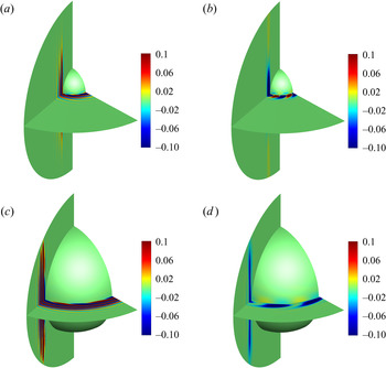
 ${p^{\prime } \boldsymbol {\nabla } \boldsymbol {\cdot } \boldsymbol {u}^{\prime }}/{\epsilon }$ is mainly distributed in the region of drifting columnar rolls aligned with the axis of rotation in both modes, and thus it is more widely distributed in the columnar mode. The change of radius ratio has no qualitative effect. Figure 17 further shows the spatial distributions of
 $p^{\prime }$ and
 $\boldsymbol {\nabla }\boldsymbol {\cdot } \boldsymbol {u}^{\prime }$ at
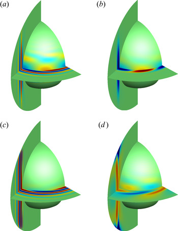
 $\eta =0.6$. For the two modes, it is found the difference in phase leads to the difference in sign of the term
 $W_p$. In the columnar mode,
 $p^{\prime }$ and
 $\boldsymbol {\nabla } \boldsymbol {\cdot } \boldsymbol {u}^{\prime }$ have the same phase in most areas, leading to a positive
 $W_p$. However, in the quasi-geostrophic compressible mode, the phases of
 $p^{\prime }$ and
 $\boldsymbol {\nabla }\boldsymbol {\cdot } \boldsymbol {u}^{\prime }$ are almost opposite in a large portion of the domain, hence the term
 $W_p$ does a net negative work, which tends to stabilize the flow.
Distribution of  ${p^{\prime } \boldsymbol {\nabla } \boldsymbol {\cdot } \boldsymbol {u}^{\prime }}/{\epsilon }$ normalized by the maximum value of
 ${\rho ^{\prime } \hat {r} \boldsymbol {\cdot } \boldsymbol {u}^{\prime } }/{\epsilon (1-\eta )^{2}r^{2}}$ for
 $Ta=10^{10}$,
 $m=5$ at
 $\eta =0.2$ (a,b) and
 $\eta =0.6$ (c,d) for two different modes: (a,c)
 $Pr=0.8, N_{\rho }=3. 0$, the columnar mode (CM); (b,d)
 $Pr=0.1, N_{\rho }=3. 0$, the quasi-geostrophic compressible mode (QCM).

Distributions of  $p^{\prime }$ (a,b) and
 $\boldsymbol {\nabla }\boldsymbol {\cdot } \boldsymbol {u}^{\prime }$ (c,d) at
 $Ta=10^{10}, \eta =0.6, m=5$: (a,c)
 $Pr=0.8, N_{\rho }=3.0$, the columnar mode (CM); (b,d)
 $Pr=0.1, N_{\rho }=3. 0$, the quasi-geostrophic compressible mode (QCM).

4. Summary and conclusions
This study systematically investigates the influence of  $\eta$ on the instability processes of fully compressible convection in rapidly rotating spherical shells. In particular, we reveal the inherent mechanical mechanisms and flow instability mechanisms of various modes quantitatively, as well as the detailed influence of
 $\eta$, by detailed analysis based on the linearized perturbation equations and the Reynolds–Orr equation.
Firstly, by investigating the instability processes of the base state for a specified  $m$ and different
 $\eta$, it is found that the instability processes have a certain similarity for different
 $\eta$. The most significant finding is that the range of parameters (
 $N_\rho , Pr$) where the base state loses stability by the quasi-geostrophic compressible mode and keeps unstable is reduced as
 $\eta$ increases. In general, at large
 $N_{\rho }$, the base state loses stability by the quasi-geostrophic compressible mode and gets stable again and finally becomes unstable by the columnar mode or the inertial mode, and the range of parameters for this kind of instability process is enlarged as
 $\eta$ increases.
Secondly, we find that the critical parameters are significantly influenced by  $\eta$. As
 $\eta$ increases, the
 $Ra_c$ and
 $m_c$ increase with
 $\eta$, which means the increase of
 $\eta$ tends to enhance the flow stability. For the same instability mode, the asymptotic scaling behaviours of
 $Ra_c$ and
 $m_c$ with
 $Ta$ can be observed, and the scaling exponents of the columnar mode and the quasi-geostrophic compressible mode are quite close for different
 $\eta$.
Finally, the linearized perturbation equations and the Reynolds–Orr equation are employed to reveal the mechanical mechanisms and flow instability mechanisms. In the quasi-geostrophic compressible mode, the time-derivative term of disturbance density in the continuity equation and the diffusion term of disturbance temperature in the energy equation are found to be very crucial, which can be ignored in the columnar mode and inertial mode, suggesting that the anelastic approximation would fail to capture the quasi-geostrophic compressible mode due to the elimination of the time-derivative term of disturbance density. In addition, the contributions of these terms become more significant as  $\eta$ increases. The disturbance momentum equation is primarily governed by the Coriolis force and pressure gradient irrespective of
 $\eta$ for all instability modes for the parameters considered. Based on the Reynolds–Orr equation, we find that, in the quasi-geostrophic compressible mode, the disturbance pressure does a net negative work instead of a net positive amount of work in the columnar mode. This finding indicates that in the quasi-geostrophic compressible mode, the disturbance pressure tends to stabilize the flow while it tends to destabilize the flow in the columnar mode. As
 $\eta$ increases, in the columnar mode, the relative work performed by disturbance pressure decreases and in the quasi-geostrophic compressible mode increases. This may explain why in a system with a larger
 $\eta$, the unstable quasi-geostrophic compressible mode is more difficult to find over a wide range of
 $Ra$. In short, in the quasi-geostrophic compressible mode, the action of the buoyancy force is the only source of instability, while there are two sources of instability in the columnar mode, i.e. the action of the buoyancy force and the work performed by the disturbance pressure. This may also explain why the columnar mode can frequently be found.
Funding
This work is supported by the National Natural Science Foundation of China under Grants 11772323, 91952103 and 11621202, the Fundamental Research Funds for the Central Universities, and the USTC Research Funds of the Double First-Class Initiative. The numerical calculations in this paper have been done on the supercomputing system in the Supercomputing Center of USTC.
Declaration of interests
The authors report no conflict of interest.
Appendix A
Here, we present the derivation of the transport equation of perturbed kinetic energy of fluid. For the fully compressible convection, the kinetic energy of fluid  $K$ can be written as
 \begin{equation} K=\tfrac{1}{2}\rho\boldsymbol{u}^{\prime} \boldsymbol{\cdot} \boldsymbol{u}^{\prime} =\tfrac{1}{2}(\bar{\rho}+\rho^{\prime})\boldsymbol{u}^{\prime} \boldsymbol{\cdot} \boldsymbol{u}^{\prime} \approx \tfrac{1}{2} \bar{\rho} \boldsymbol{u}^{\prime} \boldsymbol{\cdot} \boldsymbol{u}^{\prime}. \end{equation}
Here, we only care about the flow in the linear instability stage, so the higher-order term is ignored. The material derivative of kinetic energy is
 \begin{equation} \frac{\textrm{D} K}{\textrm{D} t} = \frac{\partial K}{\partial t} + \boldsymbol{u}^{\prime} \boldsymbol{\cdot} \boldsymbol{\nabla} K \approx \frac{\partial K}{\partial t} = \bar{\rho}\boldsymbol{u}^{\prime} \boldsymbol{\cdot} \frac{\partial \boldsymbol{u}^{\prime} }{\partial t}. \end{equation}
Then, multiplying the momentum equation by  $\boldsymbol {u}^{\prime }$, we can get
 \begin{align}
\bar{\rho} \frac{\partial \boldsymbol{u}^{\prime}}{\partial
t} \boldsymbol{\cdot} \boldsymbol{u}^{\prime}
&={-}\sqrt{\frac{P r T a}{R a}} \bar{\rho} (\hat{z} \times
\boldsymbol{u}^{\prime}) \boldsymbol{\cdot}
\boldsymbol{u}^{\prime} - \frac{\boldsymbol{\nabla}
p^{\prime}}{\epsilon} \boldsymbol{\cdot}
\boldsymbol{u}^{\prime} -\frac{\rho^{\prime}
\boldsymbol{r}}{\epsilon(1-\eta)^{2} r^{3}}
\boldsymbol{\cdot} \boldsymbol{u}^{\prime}\nonumber\\
&\quad +\sqrt{\frac{P r}{R a}}\left[\nabla^{2}
\boldsymbol{u}^{\prime}+\frac{1}{3}
\boldsymbol{\nabla}\left(\boldsymbol{\nabla}\boldsymbol{\cdot}
\boldsymbol{u}^{\prime}\right)\right] \boldsymbol{\cdot}
\boldsymbol{u}^{\prime}\nonumber\\ &=\frac{p^{\prime}
\boldsymbol{\nabla} \boldsymbol{\cdot}
\boldsymbol{u}^{\prime}}{\epsilon} - \sqrt{\frac{Pr}{Ra}}
|\boldsymbol{\nabla} \boldsymbol{u}^{\prime}|^{2}
-\frac{1}{3} \sqrt{\frac{Pr}{Ra}} (\boldsymbol{\nabla}
\boldsymbol{\cdot} \boldsymbol{u}^{\prime})^{2} -
\frac{\rho^{\prime} \boldsymbol{r} \boldsymbol{\cdot}
\boldsymbol{u}^{\prime}
}{\epsilon(1-\eta)^{2}r^{3}}\nonumber\\ &\quad
+\boldsymbol{\nabla} \boldsymbol{\cdot}
\left[-\frac{p^{\prime} \boldsymbol{u}^{\prime}}{\epsilon}
+\sqrt{\frac{Pr}{Ra}} \boldsymbol{\nabla}
\boldsymbol{u}^{\prime} \boldsymbol{\cdot}
\boldsymbol{u}^{\prime}+\frac{1}{3}\sqrt{\frac{Pr}{Ra}}\boldsymbol{u}^{\prime}
(\boldsymbol{\nabla} \boldsymbol{\cdot}
\boldsymbol{u}^{\prime})\right].
\end{align}
Furthermore, to integrate the equation (A3) over the entire sphere shell  $V$, one can obtain
 \begin{align} \int_{V} \bar{\rho}
\frac{\partial \boldsymbol{u}^{\prime}}{\partial t}
\boldsymbol{\cdot} \boldsymbol{u}^{\prime} \,\textrm{d}V &=
\int_{V} \boldsymbol{\nabla} \boldsymbol{\cdot}
\left[{-}p^{\prime} \boldsymbol{u}^{\prime}
+\sqrt{\frac{Pr}{Ra}} \nabla \boldsymbol{u}^{\prime}
\boldsymbol{\cdot}
\boldsymbol{u}^{\prime}+\frac{1}{3}\sqrt{\frac{Pr}{Ra}}\boldsymbol{u}^{\prime}
(\boldsymbol{\nabla} \boldsymbol{\cdot}
\boldsymbol{u}^{\prime})\right] \textrm{d}V +\int_{V}
\frac{p^{\prime} \boldsymbol{\nabla}\boldsymbol{\cdot}
\boldsymbol{u}^{\prime}}{\epsilon} \textrm{d}V\nonumber\\
&\quad -\int_{V} \sqrt{\frac{Pr}{Ra}} |\boldsymbol{\nabla}
\boldsymbol{u}^{\prime}|^{2} \,\textrm{d}V -\int_{V}
\frac{1}{3} \sqrt{\frac{Pr}{Ra}}
(\boldsymbol{\nabla}\boldsymbol{\cdot}
\boldsymbol{u}^{\prime})^{2} \,\textrm{d}V-\int_{V}
\frac{\rho^{\prime} \hat{r} \boldsymbol{\cdot}
\boldsymbol{u}^{\prime}}{\epsilon(1-\eta)^{2}r^{2}}
\textrm{d}V. \end{align}
Then, we can get the fully compressible Reynolds–Orr equation
 \begin{equation} K_{t}=\int_{V} \bar{\rho} \frac{\partial \boldsymbol{u}^{\prime}}{\partial t} \boldsymbol{\cdot} \boldsymbol{u}^{\prime} \,\textrm{d}V=W_{p}+\omega_{1}+\omega_{2}+B, \end{equation}
where
 \begin{equation} \left.\begin{gathered} W_{p}=\int_{V} \frac{p^{\prime} \boldsymbol{\nabla} \boldsymbol{\cdot} \boldsymbol{u}^{\prime}}{\epsilon} \textrm{d}V;\\ B={-}\int_{V} \frac{\rho^{\prime} \hat{r} \boldsymbol{\cdot} \boldsymbol{u}^{\prime} }{\epsilon(1-\eta)^{2}r^{2}} \textrm{d}V;\\ \omega_{1}={-}\sqrt{\frac{Pr}{Ra}}\int_{V} |\boldsymbol{\nabla} \boldsymbol{u}^{\prime}|^{2} \,\textrm{d}V;\\ \omega_{2}={-}\frac{1}{3} \sqrt{\frac{Pr}{Ra}}\int_{V} (\boldsymbol{\nabla}\boldsymbol{\cdot} \boldsymbol{u}^{\prime})^{2}\,\textrm{d}V. \end{gathered}\right\} \end{equation}