Observables

We begin by defining two quantities: t _h is the total duration of a planet's habitable era, and t _e is the time it would take for observers to emerge on a habitable planet given an indefinite amount of time to do so. Our planet has been capable of supporting life for approximately 4 Gyr, but it is unclear when it will become inhospitable. Climate models typically project catastrophic temperature rises in approximately 1 billion years time (excluding any anthropogenic influence). Throughout this work we shall simply assume that our two observed values are given by t _e ≃ 4 Gyr and t _h ≃ 5 Gyr. As we are less concerned with absolute values, this data can be more concisely expressed as the fractional emergence time τ ≡ t _e / t _h. Our observed value is therefore ${\rm \tau} _ \oplus \simeq 0.8$ .

The biased observation of habitable and evolutionary timescales

The ensemble of habitable and evolutionary timescales, t _h and t _e, form probability distributions denoted by $p(t_{\rm h})$ and $p(t_{\rm e})$ . The potential for correlations to exist between t _h and t _e has been discussed previously by Livio (Reference Livio1999), but here we shall treat them as independent variables. For simplicity we also assume that the mean number of observers does not strongly depend on these variables.

The observed duration of a host planet's habitable era, ${p}^{\prime}(t_{\rm h})$ , is related to the true distribution as follows

(1) $${\,p}^{\prime}(t_{\rm h}) \propto p(t_{\rm h})\int_0^{t_{\rm h}} p(t_{\rm e})\,{\rm d}t_{\rm e}.$$

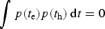
Unsurprisingly, longer habitable eras are more likely to be observed than short ones. One could never observe a habitable period that was briefer than the fastest evolutionary timescale. The habitable era of an observer's host planet is therefore a biased estimator for the typical duration of other habitable eras (unless the functions are orthogonal, $\int p(t_{\rm e})p(t_{\rm h})\,{\rm d}t = 0$ ). Similarly the probability distribution for the observed emergence time ${p}^{\prime}(t_{\rm e})$ is

(2) $${\,p}^{\prime}(t_{\rm e}) \propto p(t_{\rm e})\int_{t_{\rm e}}^\infty p(t_{\rm h})\,{\rm d}t_{\rm h},$$

illustrating that fast evolutionary paths are more likely to succeed, and thus be observed, than slow ones.

Since the observed values of t _h and t _e are similar, t _e = 0.8t _h, this implies that ${p}^{\prime}(t_{\rm h})$ and ${p}^{\prime}(t_{\rm e})$ are likely to be strongly localized functions, in that they possess similar means and small variances. This would ensure that a typical population of observers will appear after a significant fraction of the planet's habitable era.

The true probability distributions $p(t_{\rm h})$ and $p(t_{\rm e})$ could involve timescales, which differ by many orders of magnitude. We shall therefore refer to the means and variances of their logarithmic distributions, denoted by μ_h and ${\rm \sigma} _{\rm h}^2 $ respectively. In general there are three scenarios, which generate narrow distributions in ${p}^{\prime}(t_{\rm h})$ and ${p}^{\prime}(t_{\rm e})$ :

1. (a) There exists a broad range of evolutionary timescales, whose probability distribution $p(\log t_{\rm e})$ rises rapidly prior to the timescale of the typical habitable period.

2. (b) There exists a broad range of habitable periods, whose probability distribution $p(\log t_{\rm h})$ falls rapidly beyond the typical evolutionary timescale.

3. (c) The two distributions are, by coincidence, both narrow ( ${\rm \sigma} _{\rm h}^2 \lesssim 1$ ; ${\rm \sigma} _{\rm e}^2 \lesssim 1$ ) and possess similar characteristic timescales (μ_h ≃ μ_e).

Hypothesis (c) demands a high degree of fine-tuning, so we shall not consider it further. The remaining two possibilities suggest that at least one of the following statements is true: either mankind emerged unusually quickly (μ_e ≫ 4 Gyr and ${\rm \sigma} _{\rm e}^2 \gg 1$ ), or the Earth has an unusually long habitable period compared with most other habitable planets (μ_h ≪ 5 Gyr and ${\rm \sigma} _{\rm h}^2 \gg 1$ ).

The degree of overlap between $p(t_{\rm h})$ and $p(t_{\rm e})$ determines the fraction of habitable planets, which at some point harbour observers, f _o,

(3) $$\eqalign{\,f_{\rm o} & = p(t_{\rm e} \lt t_{\rm h}) \cr & = \int_0^\infty p(t_{\rm h})\int_0^{t_{\rm h}} p(t_{\rm e})\,{\rm d}t_{\rm e}\,{\rm d}t_{\rm h}.} $$

Given that μ_h ≪ μ_e, this ensures f _o ≪ 1, meaning that the emergence of observers is a rare event among habitable planets. This conclusion holds for both hypotheses (a) and (b). However they differ radically in their predictions for planets which are habitable at the present time. Now we exclude planets, which are either no longer habitable, such as Mars, or are yet to become habitable. The fraction of currently habitable planets, which produce intelligent life, f _t , is given by

(4) $$\eqalign{\,f_t & = p(t_{\rm e} \lt t_{\rm h} \vert h) \cr & = p(t_{\rm e} \lt t_{\rm h})p(h \vert t_{\rm e} \lt t_{\rm h}) \cr & = \displaystyle{{\int_0^\infty t_{\rm h}p(t_{\rm h})\int_0^{t_{\rm h}} p(t_{\rm e})\,{\rm d}t_{\rm e}\,{\rm d}t_{\rm h}} \over {\int_0^\infty t_{\rm h}p(t_{\rm h})\,{\rm d}t_{\rm h}}}.} $$

Now the long evolutionary timescale μ_h ≪ μ_e no longer implies a sparse habitation of habitable planets f _t  ≪ 1. In fact, provided the variance of habitable periods ${\rm \sigma} _{\rm h}^2 $ is sufficiently large, the habitation fraction f _t approaches unity. This result considerably boosts the prospects for search for extra-terrestrial intelligence (SETI) experiments, which would otherwise appear bleak if all habitable periods were identical ( ${\rm \sigma} _{\rm h}^2 = 0$ ). Note that ${\rm \sigma} _{\rm h}^2 = 0$ had been implicitly assumed in previous studies. By relaxing this assumption, we are no longer drawn to the conclusion that the vast majority of habitable exoplanets are devoid of intelligent life. The alternative interpretation is that there were many other planets, such as Mars, which remained habitable for relatively brief periods.

Late emergence

We now briefly demonstrate how variability in the duration of habitable periods can lead to the first observers appearing in the latter half of their planet's habitable period. For our toy model we adopt $p(t_{\rm e}) = {\rm \delta} _K(t_{\rm e} - T_E)$ , where T _E  = 4 Gyr. In other words, advanced life always requires 4 billion years to emerge. If the distribution of habitable periods can be described as a power law when t _h > T _E then

(5) $$p(t_{\rm h}) \propto t_{\rm h}^{ - \alpha} \;(t_{\rm h} \gt T_E),$$

while its behaviour for t _h < T _E has no bearing on the observed distribution. For α > 2, the expected habitable time can then be derived from (1)

(6) $$E(t_{\rm h}) = \displaystyle{{{\rm \alpha} - 1} \over {{\rm \alpha} - 2}}T_E.$$

Provided the power law is sufficiently steep $({\rm \alpha} \gt 3)$ then $E(t_{\rm h}) \lt 2T_E$ , so the first observers are not expected to appear until the latter stages of the habitable era.

Hard step model revisited

In this section we explore the consequences of scenario (a), as defined above in the section ‘The biased observation of habitable and evolutionary timescales’. In particular, we focus on the hard step model originally proposed by Carter & McCrea (Reference Carter and McCrea1983). How many unlikely hurdles must be overcome before an intelligent species can emerge? This number has important implications for the abundance of life in the Universe. If there is just a single hard step prohibiting the formation of intelligent life, then there are grounds to believe that primitive life arises frequently. The relatively rapidFootnote ¹ emergence of life on Earth has been interpreted as evidence that abiogenesis is a relatively straightforward process (Lineweaver & Davis Reference Lineweaver and Davis2002). However, if abiogenesis was the first of several hard steps, then even primitive life is a rare occurrence (Hanson Reference Hanson1998). The stark contrast between the predictions of the single-step and multiple-step models motivates us to utilize model selection. The purpose of model selection is to identify which model offers the best fit to the data, while accounting for the complexity or predictiveness of the model.

For N hard steps, the probability that success occurs at a fractional time τ is given by (Carter Reference Carter2008)

(7) $$p({\rm \tau} \vert N) = \displaystyle{{N!{\rm \tau} ^{r - 1}{({\rm \tau} - 1)}^{N - r}} \over {(r - 1)!(N - r)!}}.$$

If N = 1 this is constant, implying that observers are equally likely to emerge at any given time, while for N > 1 the function peaks at τ = 1. To compare the single step model $(N = 1)$ with the multi-step case, where N is a free parameter, we evaluate the Akaike Information Criterion (AIC), defined as

(8) $${\rm AIC} = 2k - 2\log ({\rm {\cal L}}),$$

where ${\rm {\cal L}}$ is the maximum likelihood and k is the number of free parameters (Akaike Reference Akaike1974). For the single step model we find AIC_s = 5.66, while the multi-step model yields AIC_m = 6.23, with the maximum likelihood achieved with N = 5. The relative likelihood is given by ${\rm exp}(({\rm AI}{\rm C}_{\rm s} - {\rm AI}{\rm C}_{\rm m})/2) = 0.75$ . The multi-step model is therefore weakly disfavoured relative to the simpler single-step case. If we were to adopt the Bayesian Information Criterion (BIC, Schwarz Reference Schwarz1978), the multi-step model would be more heavily penalised. Therefore, even within the context of the hard step model, there is no evidence to suggest that abiogenesis is a slow process, or a rare event.

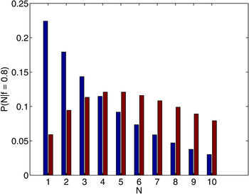
Figure 1 provides an illustration of why there was insufficient evidence to invoke a new parameter in the model to fit the data. The two sets of bars displays the posterior probability $p(N\vert {\rm \tau} = 0.8)$ for two different choices of prior $p(N)$ . The posterior is given by Bayes’ theorem

(9) $$p(N \vert {\rm \tau} ) = \displaystyle{{\,p({\rm \tau} \vert N)p(N)} \over {\,p({\rm \tau} )}}.$$

Fig. 1.

In the context of the hard step model, the posterior probability of N hard steps based on the observation of a single success arising at $80\% $ of the maximum time available. The left-hand set of bars are derived from an uninformative prior $p(N) \propto 1/N$ , while adopting a flat prior yields the second set of bars.

The left set of bars represent the case $p(N) \propto 1/N$ , the conventional choice for an uninformative prior, while the second set of bars corresponds to a uniform prior. In each case, it is evident that N = 1 is not significantly disfavoured.

Easy stroll model

The formation of the Earth did not require billions of years because it was an improbable event – many other planets formed on a similar timescale – it required billions of years because it involved fundamentally slow processes. These include the collapse of cosmic structure, the lifespan of the first stars, and the growth of planetesimals. Similarly, the development time for mankind may have been limited by a slow process rather than a difficult one. This corresponds to scenario (b) (see the section ‘The biased observation of habitable and evolutionary timescales’) where habitable periods vary by several orders of magnitude, while evolutionary timescales are more consistent.

The evolutionary trajectory from a primordial microbe to our macroscopic form demanded a change in organism size of over 16 orders of magnitude. How rapidly could we realistically expect this transformation to take place? One of the fastest cases of gigantification to be well documented is the trajectory followed by cetacea. Over the past 50 million years the blue whale has maintained a remarkable growth rate, increasing in body mass by three orders of magnitude (Montgomery et al. Reference Montgomery2013). Even if we use this extraordinary individual example as a benchmark, at this rate we would still require over 250 million years to rise 16 orders of magnitude in body mass. The mean enlargement rate of the largest organism is likely to be substantially slower than it was for this particular mammal over this relatively brief timespan. It therefore appears feasible that the evolution of sufficiently large human precursors invariably takes several billion years, thereby acting as our rate-limiting step, as opposed to other obstacles such as encephalisation.

The size requirement is not a unique problem for our species, but presents a more general problem for all observers. To be classified as an observer, an organism must exceed some minimum degree of complexity, and with that requirement comes a minimum brain size. Even if we conservatively set a minimum observer body mass of 1 kg – less than the mass of the human brain – this still leaves a formidable 15 orders of magnitude to climb. Further justification for this mass limit comes from an independent calculation, which exploits the relationship between body size and population density. Simpson (Reference Simpson2016) estimated the minimum mass of a given species of observer to be m > 25 kg (95% confidence limit).

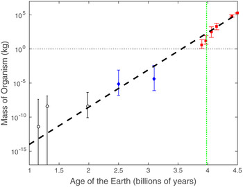
Figure 2 maps the enlargement of some of the Earth's largest organisms across a logarithmic mass scale. The plotted points reflect the largest known species of their time, which can be well determined at late times but our confidence prior to the onset of the Cambrian explosion (vertical dashed line) is considerably weaker. The earliest evidence for living organisms comes from Wacey et al. (Reference Wacey2011), Javaux et al. (Reference Javaux2010), and Czaja (Reference Czaja2016). The earliest recorded macroscopic species is Grypania (Runnegar Reference Runnegar1991; Han & Runnegar Reference Han and Runnegar1992), but again we cannot be certain either that we have truly found the largest organism of its time, or if it consists of a colony of smaller organisms. The tail of the mass distribution is highly extended, meaning that even a small degree of incompleteness can lead us to significantly underestimate the size of the largest species.

Fig. 2.

The exponential enlargement of species over the past 4 billion years. The three hollow black circles relate to the organic-walled microfossils presented in Javaux et al. (Reference Javaux2010); Wacey et al. (Reference Wacey2011), and Czaja (Reference Czaja2016), respectively. The upper error bars represent our highly incomplete state of knowledge for organisms at that time, while the lower error bars reflect the possibility that the microfossils comprise colonies of smaller organisms. The two blue diamonds correspond to specimens of Grypania, thought to be a eukaryotic alga, dated at 1.4 and 2.1 Gyr (Runnegar Reference Runnegar1991; Han & Runnegar Reference Han and Runnegar1992). The six red squares correspond to the largest animal species of their time, from left to right: Anomalocaris; Dickinsonia Rex; Cameroceras; Rhizodus; Argentinasaurus; and the blue whale. The diagonal dashed line ilustrates the trajectory expected from the simplest diffusion model, as specified by equation (10). The vertical dashed line marks the onset of the Cambrian explosion, associated with the emergence of numerous macroscopic species.Footnote ²

At late times we focus on the largest species within the animal kingdom, where fossil records show a progressive enlargement, from Anomalocaris, Dickinsonia Rex, Cameroceras, Rhizodus and Argentinasaurus, while the present day is represented by the blue whale. Note that the plant kingdom followed a very similar growth pattern, as illustrated in Fig. 1 of Payne et al. (Reference Payne2009).

The spread of the biosphere's mass function (which we define as the abundance of biomass as a function of the organism's body mass) appears to have been broadly consistent with an exponential growth law. This behaviour is to be expected from a multiplicative diffusion process, a model which has been substantiated by the diversification of mammalian species (Clauset & Redner Reference Clauset and Redner2009) and the observed distributions of inter-species and intra-species body masses (Clauset & Erwin Reference Clauset and Erwin2008).

Payne et al. (Reference Payne2009) concluded that the fossil records are highly inconsistent with a simple diffusion model. This was partially based on the assertion that a random walk progresses in proportion to the square root of time. However in a random walk it is the median path, not the maximum path, which propagates as the square root of the number of steps taken. The maximum path evolves approximately linearly with time, as illustrated by the solid line in Fig. 2. If the maximum organism mass is denoted by m then its evolution with time may be parameterized asFootnote ²

(10) $$m = m_0\,{\rm e}^{t/{\rm \tau}}. $$

where m ₀ is the initial organism size at time t = 0, ${\rm \tau} = \ln (2)t_2$ is the growth constant, and t ₂ is the timescale for the maximum organism size to double. For Fig. 2 we adopt a doubling time of t ₂ = 55 million years, as shown by the dashed line.

Now we consider the error bars attributed to the data points. For larger and more recent species the detection efficiency is expected to be high. However it seems extremely unlikely that the detection efficiency remains as high for the older microscopic organisms. For example, the fossils of the largest known dinosaur species were found not by paleontologists but a local farm worker. Such serendipitous finds clearly cannot occur with microfossils. Furthermore it can be difficult to distinguish a single large microorganism from a colony of smaller microorganisms. We therefore limit ourselves to a few early cases prokayotes and eukarotes, and attribute large uncertainties to the upper bound of their masses. Note that unlike Payne et al. (Reference Payne2009), we do not include the 3.5 Gyr Primaevifilum (Schopf & Packer Reference Schopf and Packer1987), since recent studies have found these morphologies to be consistent with mineral artefacts (Brasier et al. Reference Brasier2015; Wacey et al. Reference Wacey2015). Instead we consider the 3.2 – 3.4 Gyr cases documented by Javaux et al. (Reference Javaux2010), Wacey et al. (Reference Wacey2011), Sugitani et al. (Reference Sugitani2015), and the 2.5 Gyr samples from Czaja (Reference Czaja2016). These studies were all published in the last few years, indicating the rapid development of the field.

Of the macroscopic species shown, only Cameroceras has a poorly determined mass. The size of this mollusc is extremely challenging to estimate. For the largest candidates, only small shell fragments have been found, leading to conflicting extrapolations of its full size. A further complication is that around 90% of its volume consists of a hollow shell, rather than biological tissue.

There were undoubtedly a number of key events along this trajectory such as the first cell nucleus, the Great Oxygenation Event and various mass extinctions (Szathmáry & Smith Reference Szathmáry and Smith1997; Szathmary & Smith Reference Szathmary and Smith2000). However it is often the case that simple scaling behaviours emerge from highly complex systems. For example, over the past 50 years the development of semiconductor technologies has adhered to the smooth progression of Moore's Law, despite relying upon a series of individual breakthroughs such as the invention of photolithography.