INTRODUCTION
Disturbances are common to most, if not all, mature forest communities and they represent a crucial component in the maintenance of its pattern and processes (van der Maarel Reference VAN DER MAAREL1993). In tropical forests, disturbance activities are mainly represented by the death of part of a tree, of a whole tree or of several trees. Due to internal (e.g. diseases) and/or external causes (e.g. wind), trees mostly fall by uprooting or stem breakage (Arriaga Reference ARRIAGA2000, Runkle Reference RUNKLE1982, van der Meer & Bongers Reference VAN DER MEER and BONGERS1996a). Yet, trees can still die standing and gradually decompose its crown. Branch-falls and inclined trees can also occur, though they are not related to the death of an individual. Each one of these modes of disturbance has its own consequences on light transmission, understorey vegetation and soil disturbance (Clark Reference CLARK, Bawa and Hadley1990). Openings in the canopy may be formed as a consequence of tree death and their influence on forest structure and regeneration are broadly known (Busing Reference BUSING2005, Denslow Reference DENSLOW1980, Hubbell & Foster Reference HUBBELL, FOSTER and Crawley1986). However, not all events of tree mortality result in canopy gaps (Poore Reference POORE1968, van der Meer & Bongers Reference VAN DER MEER and BONGERS1996a). Lieberman et al. (Reference LIEBERMAN, LIEBERMAN, PERALTA and HARTSHORN1985) estimated that at least half of the dead trees bigger than 10 cm diameter at breast height (dbh) were not associated with canopy gaps.
The community pattern of tree mortality, known as forest disturbance regime, is regarded as a good descriptor of forest structure and regeneration (Clark Reference CLARK, Bawa and Hadley1990). Its description is usually done in two different ways. One is based on tree individual mortality and its consequences (Busing Reference BUSING2005, Lieberman et al. Reference LIEBERMAN, LIEBERMAN, PERALTA and HARTSHORN1985) and the other comprises the description of the number, average size, frequency and spatial distribution of canopy gaps (Brokaw Reference BROKAW, Leigh, Rand and Windsor1982b, Grau Reference GRAU2002, Kapos et al. Reference KAPOS, PALLANT, BIEN and FRESKOS1990). More complete studies involve the association of both approaches (van der Meer & Bongers Reference VAN DER MEER and BONGERS1996a) and the recording of gap expansion processes (Runkle Reference RUNKLE1990, Tanaka & Nakashizuka Reference TANAKA and NAKASHIZUKA1994). An alternative approach in describing the disturbance regime is estimating the forest turnover rate, defined as the mean time between the formation of successive gaps on the same forest spot (Poore Reference POORE1968). The calculation is normally based either on the rate of gap formation (Hartshorn Reference HARTSHORN, Tomlinson and Zimmermann1978) or on the rate of tree mortality (Lieberman et al. Reference LIEBERMAN, LIEBERMAN, PERALTA and HARTSHORN1985).
Although considered a good index in assessing forest dynamics (Denslow Reference DENSLOW1980), authors point out practical limitations of turnover estimation related to gap delimitation and measurement methods (Lima Reference LIMA2005, van der Meer et al. Reference VAN DER MEER, BONGERS, CHATROU and RIERA1994), to the exception of repeated disturbances events (Riera & Alexandre Reference RIERA and ALEXANDRE1988) and to the fact that many treefalls do not create canopy gaps (Lieberman et al. Reference LIEBERMAN, LIEBERMAN, PERALTA and HARTSHORN1985, Martini et al. Reference MARTINI, LIMA, FRANCO and RODRIGUES2007). In tropical semi-deciduous forests, where seasonal fluctuations in canopy cover are inherent to forest functioning, the influence of gap processes on forest dynamics may be of less importance (Denslow & Hartshorn Reference DENSLOW, HARTSHORN, McDade, Bawa, Hespenheide and Hartshorn1994). Although seasonal fluctuations in canopy cover overshadow the influence of gap processes on forest dynamics, studies emphasizing the subject are very scarce for this forest formation. In this paper we assess the canopy disturbance regime in a tropical semi-deciduous forest in south-eastern Brazil. By means of an exhaustive recording of canopy gaps, we attempt to evaluate size, age and size-class frequencies of such openings and the gap makers related to them. More specifically, we addressed the following questions: How do gap delimitation methods and repeated disturbances influence the estimation of canopy turnover rate and other disturbance regime descriptors? And what are the main factors controlling gap size?
SITE DESCRIPTION
This study was carried out in the Estação Ecológica de Caetetus (EEC), a state forest reserve which belongs to Gália county (22°41′S and 49°10′W). It has a total area of 2178 ha covered by an old-growth semi-deciduous seasonal forest, with a canopy height ranging from 20 to 35 m. The terrain is flat, with elevation ranging from 550 to 650 m asl. The soil is red-yellow Acrisols (Ultisols) and red-yellow Ferrasols (Oxisols) but haplic Gleysols (Entisols) can be found on the lowest points of the landscape. Average annual precipitation is around 1400 mm and characterized by the occurrence of a marked dry season. The average annual temperature is 21 °C. Near the centre of the reserve, a permanent plot of 10.24 ha was established in 2002 to study forest composition and dynamics. In the 2005 plot census, 12 039 individuals > 5 cm dbh were sampled, belonging to 148 species, 110 genera and 44 families. Plot basal area was 36.8 m2 ha−1. The richest families were Myrtaceae, Euphorbiaceae, Fabaceae, Mimosaceae and Rutaceae, and the five most abundant species were Metrodorea nigra, Ocotea indecora, Trichilia clausenii, Aspidosperma polyneuron and Trichilia catigua.
METHODS
In 2005, 8.96 ha (280 × 320 m) of the permanent plot was completely surveyed for canopy gaps during the dry season. The canopy gap definition used followed Runkle (Reference RUNKLE1992) who defines a gap as formed by the death (absence from the canopy) of at least one-half of a tree. Additionally, we marked and measured canopy openings, defined here as openings in the canopy without past or present evidence of the death of gap makers. Large gaps that exceeded the plot limits were not completely measured and only the area inside the plot was used to estimate the total plot gap area. In contrast, smaller gaps with some portions outside gap limits were measured completely and used in the gap area analyses, as explained below.
Once the canopy gap or opening were located, we used two different methods to set its limits: Brokaw (Reference BROKAW, Leigh, Rand and Windsor1982a: the vertical projection of the ‘hole in the forest extending through all levels down to an average height of two meters above ground’) and Runkle (Reference RUNKLE1982: ‘the ground area under a canopy opening extending to the bases of canopy trees surrounding the canopy opening’), referred from now on simply as Brokaw and Runkle methods, respectively. Thus, for each gap, we obtained the area directly above the canopy gap and the expanded gap area. Each method was applied by the same observer to avoid bias. We set 10 m2 as a minimum gap size and a minimum size of 20 cm dbh to define the surrounding canopy trees. The size of each canopy gap was measured using the method proposed by Lima (Reference LIMA2005). Exceptions were made for three large gaps that had part of their area outside the study plot. In these cases, we noted the tag number of all bordering canopy trees and size measurement by Runkle's method was made a posteriori based on their coordinates. Gap size inside the plot was then obtained by the area of the polygon, linking all bordering canopy trees sketched using a graphic editor program (Arc View GIS 3.3). Hence, Brokaw gap size was estimated based on the regression equation obtained comparing both delimitation methods.
For each gap, we set an arbitrary centre inside Brokaw's limits, from which all measures were taken using a DME 201 (Haglöf Sweden AB). Next, we made a complete survey for gap makers (i.e. all dead trees or branch falls > 20 cm dbh) that were identified (whenever possible) and measured for dbh and mode of disturbance (uprooting, snapping, standing dead, fall of a stem from multi-stemmed trees, branch fall, inclined tree and the association of two or more modes of disturbance, hereafter called ‘complex trees’). To define gap makers in this study, the distinction between initiator and domino trees were not made due to difficulty of differentiating between them in the field, especially inside multiple-event gaps. We then made estimates of gap age, based on the presence/absence of tree identification tags on gap maker(s). Since tags were placed in 2002, we created two broad age classes: recent gaps (gaps newer than 3 y old) when the gap maker was tagged; and old gaps, when the gap maker not tagged and presented more advanced stages of wood decay. Although a 3-y-old gap may not be accurately defined as recent, the presence of tags assured an excellent time parameter because of the information it gave us for the period 2002–2005, aiding in the calculation of the disturbance and turnover rates.
Complex gaps, formed by distinct episodes of tree mortality, received a special approach as suggested by Runkle (Reference RUNKLE1992). When the spatial distinction between tree- and/or branch-fall episodes was structurally unclear, total superposition of the two fall episodes was assumed. Accordingly, the gap was regarded as a single gap with two different age classes, one relative to the first fall episode and one from the second. During analysis, when the age class was required these gaps were excluded, except for estimations of turnover rate. Complex gaps with clear spatial differentiation between fall episodes were then subdivided into two contiguous fractions (partial overlapping), each one with its own age class and area. During the estimation of turnover rate, each fraction of these gaps was used separately. The limit between these contiguous gaps was determined by considering the area of influence of each episode (with one or more gap makers), sapling height and relative decay of surrounding debris.
Data analysis
Since gap size data did not follow a normal distribution, comparisons among delimitation methods, types of gaps (single and complex gaps) and age classes (old and recent) were made by the inspection of median confidence intervals in notched box-plots. Non-overlapping confidence intervals were considered as an indication of dissimilar distributions (McGill et al. Reference McGILL, TUKEY and LARSEN1978). A regression analysis was carried out to investigate the relationship between Brokaw and Runkle methods; a non-linear model was adopted because the inclusion of the quadratic term significantly improved the model fit (df = 91, F = 6.99, P = 0.009). A standard multiple regression was also applied to evaluate the strength of number and size of gap makers on the prediction of canopy gap size. In both regression analyses, the three large canopy gaps not completely measured were not included. The evidence of different size distribution of the gap makers among the different modes of disturbance was evaluated using Analysis of Variance (ANOVA). During some of the analysis, such as regression and average comparison, a number of gaps were excluded due to partial measurement of area and contours. Canopy openings were not included in the gap size versus gap maker analysis either. Therefore, the number of gaps used varied between analyses.
We also made estimates on the gap disturbance rate (i.e. new gaps per hectare per year) to calculate the stand turnover rate, defined according to Poore (Reference POORE1968, p. 178). The mean disturbance rate was obtained by dividing the total gap area of recent gaps by the number of years since tree mortality started being recorded in 2002. The turnover rate was expressed indirectly as the number of years necessary to cover the entire plot area with gaps and calculated following Hartshorn (Reference HARTSHORN, Tomlinson and Zimmermann1978). To assess the effect of including repeated disturbances events on turnover rate, we calculated the turnover rate by adding the area of recent gaps that partly or entirely covered older gaps (complex gaps, as explained above). To compare average gap size and turnover rate to other studies, values were corrected in respect to the method of size measurement adopted, following the linear equations provided in Lima (Reference LIMA2005).
RESULTS
Disturbance regime and turnover rate
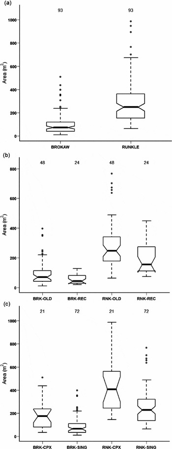
We found a total of 100 canopy gaps totally or partially inside the studied area (11.2 gaps ha−1). Among these, canopy openings were uncommon (0.8 gaps ha−1), presented smaller values than single canopy gaps (inspection of notched box-plots, data not presented) and contributed only 3.0% and 4.3% of Brokaw and Runkle total gap area, respectively. As expected, Brokaw gap areas were significantly lower than Runkle's (Figure 1a) and the quadratic regression applied revealed significant relation between methods (Runkle size = 0.00046 (Brokaw size2) + 1.94 Brokaw size + 100; r2 = 0.809; N = 93; P < 0.001). But, there was considerable deviation on individual gap sizes. For example, for a Brokaw gap size of 78 m2, a Runkle gap size of 249 m2 is expected. However, observed values varied from 158 to 448 m2.
Size distribution of canopy gaps found in a tropical semi-deciduous forest, south-eastern Brazil. Size values measured according to two different delimitation methods and separated as follows: all gaps (a), old and recent gaps (b) and single and complex gaps (i.e. gaps formed by distinct episodes of tree mortality) (c). For all figures, the centre vertical line marks the sample median. Box edges represent the first and third quartiles. Boxes are narrowed at the median and return to full width at the lower and upper confidence interval. Whiskers show the range of values that fall within 1.5 times the length of the box. Outliers are plotted as empty circles. BROKAW (or BRK) = Brokaw gap size; RUNKLE (or RNK) = Runkle gap size; SING = Single gaps; CPX = Complex gaps; OLD = Single gaps formed before 2002; REC = Single gaps formed between 2002 and 2005.

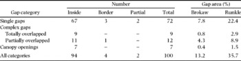
Among all gaps, we encountered 21 complex gaps (2.4 gaps ha−1) with distinct episodes of complete or partial gap overlap (Table 1). These gaps varied greatly in size from 32 and 145 m2 to 507 and 1109 m2 (Brokaw and Runkle sizes, respectively). The biggest of all gaps also corresponded to a complex gap (1004 and 1619 m2, respectively) but since we did not measure its complete area (gap largely exceeded plot limits), it and two other partially measured gaps were not used during analysis. There was strong evidence of complex gaps being bigger than single gaps for both delimitation methods (Figure 1b). Complex gaps corresponded to 21.0% of all canopy gaps found in our study plot and contributed for 4400 and 10 587 m2 (37.1 and 33.2%) of total Brokaw and Runkle gap area.
Number and categories of canopy gaps found inside 8.96-ha of tropical semi-deciduous forest in south-eastern Brazil. Inside = gaps completely measured and inside plot limits; Border = gaps completely measured but partially inside gap limits; Partial = large gaps measured only inside plot limits. Brokaw and Runkle refer to the two methods of gap delimitation employed. Complex gaps = canopy gaps formed by distinct episodes of tree mortality. Canopy openings = canopy gaps without evidence of gap makers. Values of area for all categories are corrected by subtracting gap portions outside plot limits.

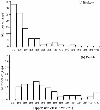
The size class frequencies (Figure 2) revealed that 77% of canopy gaps measured using the Brokaw method were smaller than 150 m2 and gaps bigger than 400 m2 were rare (3%). As expected, gaps smaller than 150 m2 had a disproportionate contribution of only 42% of total gap area. Correspondingly, 71% of all the gaps were smaller than 350 m2 but they accounted for no more than 45% of the total Runkle gap area. Moreover, there was evidence of difference in Runkle gap area between age classes but the same was not true for Brokaw method (Figure 1c). Thus, for Runkle method, older gaps were bigger than recent ones (complex gaps and canopy openings excluded from this analysis). The number and the proportionate contribution of gaps in the old age class were respectively about two and three times bigger than recent gaps, a result practically independent of the delimitation method.
Size class frequencies of canopy gaps measured applying Brokaw (a) and Runkle (b) gap delimitation methods (N = 93), in a tropical semi-deciduous forest, south-eastern Brazil. Gaps exceeding the limits of the plot (i.e. not completely measured) are not included.

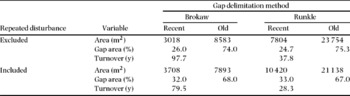
We further compared the number of gaps and the contribution to total gap area as if we had not considered repeated disturbance events. Both variables had considerable discrepancies related to the exclusion of repeated disturbances events. As a consequence of differences in total area related to the inclusion of overlapping gap areas, the turnover rates were quite different between the two situations (Table 2). The results between gap delimitation methods were different as well. The mean annual rate of newly formed gaps (i.e. disturbance rate) calculated for the three years of records was 1.1 gaps ha−1.
Total gap area and forest turnover rate calculated for both delimitation methods and for two different estimations of recent gap area: including and excluding repeated disturbance events. Brokaw and Runkle refer to the gap delimitation methods employed. Recent gap area represented by the mean gap area opened per year, calculated for a 3 years interval. Recent and old age classes are gaps newer and older than 3 y old, respectively.

Canopy gap makers
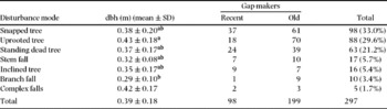
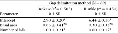
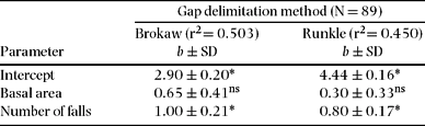
Related to 93 canopy gaps, we encountered 297 gap makers representing a median and average (± SD) of 2.0 and 3.2 ± 2.6, respectively. On account of some difficulty in measuring the dbh of some of the old fallen trees, we measured 289 gap makers (Table 3) that ranged from 0.2 (lower limit previously defined) to 1.7 m. The basal area of gap makers per gap was 0.45 ± 0.50 m2 (average ± SD, N = 93) and their total basal area was roughly 4.6 m2 ha−1. Snapping, uprooting and standing dead were the most common mode of disturbance and together accounted for 83.8% (Table 3). Uprooted trees were significantly larger in dbh than branch falls (ANOVA: N = 292, F = 3.20, P = 0.014). The multiple regression indicated that the number of gap makers and the total basal area were good predictors of gap size, for both methods (Table 4). The analysis showed a significant increase of gap area in respect to total basal area (F(1, 86) = 64.3 and 48.3 for Brokaw and Runkle sizes, respectively) but the inclusion of the number of gap makers significantly increases the variance explained by the regression (F = 22.5 and 22.1, respectively). The specific identity of the gap maker was difficult to determine due to decay of the fallen log and especially because most of them were related to old tree- or branch-fall events (67.0%). Therefore, a large number of gap makers remained with undetermined identification (N = 124). Still, the five most common species among the identified gap makers were Aspidosperma polyneuron (38), Ocotea indecora (29), Syagrus spp. (19), Metrodorea nigra and Centrolobium tomentosum (16).
Diameter at breast height (dbh) and age-class distribution of gap makers in respect to the disturbance mode considered. Different superscript letters designate significant differences between means (Tukey test: α = 0.05). The data on dbh were 1/square-root-transformed prior to ANOVA. Branch fall values correspond to the fallen branch and not to the supporting tree. Complex falls (i.e. association of different modes of disturbance) were excluded from the ANOVA.

Summary of the standard multiple regression results applied to predict gap size based on number and size of gap makers. Canopy openings (i.e. canopy gaps without evidence of gap makers) not included in the analysis. Statistics: Brokaw F (2, 86) = 43.6, P < 0.001, SE of estimate: 0.617; Runkle F (2, 86) = 35.2, P < 0.001, SE: 0.497. *P < 0.001, ns = not significant. Data log(x + 1)-transformed.
DISCUSSION
Disturbance regime
The average gap size found in this study (93 m2; value corrected to Brokaw (Reference BROKAW1982a) gap size measuring method) was comparatively larger than several rain-forest sites. This was true for forests at Nouragues (54 m2: van der Meer et al. Reference VAN DER MEER, BONGERS, CHATROU and RIERA1994), Taï (55 m2: Jans et al. Reference JANS, POORTER, VAN ROMPAEY and BONGERS1993), Carlos Botelho (56 m2: Lima Reference LIMA2005), Christmas Island (around 83 m2, Green Reference GREEN1996) and Barro Colorado (86 m2: Brokaw Reference BROKAW, Leigh, Rand and Windsor1982b). However, this difference is probably due to the presence of large gaps in the EEC, reinforcing the use of the median to compare asymmetric values such as canopy gap size. Canopy openings were not numerous and predominately small. In our study area, these areas naturally free of trees are probably very old gaps in its final stages of canopy closure. Only three of seven canopy openings had no evidence of gap makers at all and the other four presented gap makers smaller than 20 cm dbh (usually branch falls). However, the distinction of canopy openings is still important because they may resemble canopy gaps in composition and function but not in their dynamics (Runkle Reference RUNKLE1992).
As already discussed elsewhere (Popma et al. Reference POPMA, BONGERS, MARTINEZ-RAMOS and VENEKLAAS1988), different gap delimitation methods generate differences of 2.8 times on average in gap size. This result is very alike to the one obtained by van der Meer et al. (Reference VAN DER MEER, BONGERS, CHATROU and RIERA1994) comparing the same methods. Even though the regression obtained was significant, conversions of individual gap size should be made carefully due to substantial variation between the observed size values of the two delimitation methods. Among the factors that may have contributed to the production of such variation, we can cite understorey vegetation damage (e.g. number and height of surviving individuals), the presence of inclined canopy trees bordering the gap and lateral extension of tree branches (creating asymmetrical crowns around gaps).
Information on number and area of gaps formed by distinct episodes of tree mortality are still scarce in gap literature, particularly for semi-deciduous forests. Nonetheless, several authors stated that trees around gaps are more susceptible to falling for different reasons (Grau Reference GRAU2002, Hubbell & Foster Reference HUBBELL, FOSTER and Crawley1986, Young & Hubbell Reference YOUNG and HUBBELL1991, but see Runkle Reference RUNKLE1990). Runkle (Reference RUNKLE1990) found that more than 60% of gaps suffered from repeated disturbances and Riera & Alexandre (Reference RIERA and ALEXANDRE1988) found that 14% of total gap area suffered from new treefalls. In our study site such gaps represented approximately 25% of all gaps found and they contributed up to one third of total gap area.
Although repeated gap disturbances are supposed to be common (Lieberman et al. Reference LIEBERMAN, LIEBERMAN, PERALTA and HARTSHORN1985, Poore Reference POORE1968, van der Meer & Bongers Reference VAN DER MEER and BONGERS1996b, Yavitt et al. Reference YAVITT, BATTLES, LANG and KNIGHT1995), we do not know to what extent researchers have not considered complex gaps or if they simply did not notice their existence. As stated by Runkle (Reference RUNKLE1992), most researchers probably combined the sections of such gaps together into a single entity. Other researchers have consciously excluded complex gaps from their analysis according to their needs (Hartshorn Reference HARTSHORN, Tomlinson and Zimmermann1978, Runkle Reference RUNKLE1982, van der Meer et al. Reference VAN DER MEER, BONGERS, CHATROU and RIERA1994). However, this sort of treefall gap certainly influences gap regeneration in a different way (Tanaka & Nakashizuka Reference TANAKA and NAKASHIZUKA1994), especially in the time required for gap closure. Therefore, the exclusion of such gaps or the merger of their sectors into one bigger gap, will probably generate limitations of interpretation on gap disturbance regime (Runkle Reference RUNKLE1992). Despite the practical difficulties in the recognition of complex gap sectors, we strongly recommend their inclusion in future studies aiming to describe the canopy disturbance regime.
The size class distribution was quite similar to many other tropical and non-tropical forest sites (Abe et al. Reference ABE, MASAKI and NAKASHIZUKA1995, Brokaw Reference BROKAW, Leigh, Rand and Windsor1982b, Runkle Reference RUNKLE1990, van der Meer & Bongers Reference VAN DER MEER and BONGERS1996b), corroborating the pattern of canopy gap formation mainly with sizes smaller than 100 m2, median gap size commonly within 50–80 m2 size class (but see Jans et al. Reference JANS, POORTER, VAN ROMPAEY and BONGERS1993, Lertzman & Krebs Reference LERTZMAN and KREBS1991) and maximum gap size rarely more than 400 m2 (but see Sanford et al. Reference SANFORD, BRAKER and HARTSHORN1986). For instance, Green (Reference GREEN1996) and Yavitt et al. (Reference YAVITT, BATTLES, LANG and KNIGHT1995) found that 90% and 87% of all canopy gaps were smaller than 120 and 125 m2, respectively. These results are quite similar to ours if we consider the differences associated to the method of size measurement applied (Lima Reference LIMA2005). In addition, our and Lertzman & Krebs (Reference LERTZMAN and KREBS1991) results for median gap size (both around 78 m2) were comparatively greater due to differences on gap size measurement as well.
Although the decrease of gap size over time was expected due to lateral and vertical growth of trees, our data showed that older gaps tended to be larger than more recent ones for Runkle but not for Brokaw gap limits. One possible explanation would be the rate of repeated disturbances found in our study area that gradually increases gap area (Hubbell & Foster Reference HUBBELL, FOSTER and Crawley1986, Lawton & Putz Reference LAWTON and PUTZ1988, Runkle Reference RUNKLE1990, Tanaka & Nakashizuka Reference TANAKA and NAKASHIZUKA1994). Another may be related to the past activity of a catastrophic disturbance agent that generated bigger gaps during a specific period of time (Abe et al. Reference ABE, MASAKI and NAKASHIZUKA1995). The difference among methods occurred probably because Brokaw limits are more unstable over short periods of time than the Runkle method, which requires a tree to reach a certain dbh (generally 20 cm) to have any change on its limits. Still with respect to gap age, it is difficult to state if the proportion of gaps in the older age class is simply a result of natural accumulation of events or if gaps are somehow failing to regenerate. Many old canopy gaps in the study area were related to small height of internal vegetation and/or to a marked abundance of lianas and woody bamboos (probably Merostachys sp.).
Turnover rate
Values of turnover rate for different forest sites varied (average 129 y: Bongers et al. Reference BONGERS, POPMA, CASTILLO and CARABIAS1988, Chandrashekara & Ramakrishnan Reference CHANDRASHEKARA and RAMAKRISHNAN1994, Jans et al. Reference JANS, POORTER, VAN ROMPAEY and BONGERS1993, van der Meer et al. Reference VAN DER MEER, BONGERS, CHATROU and RIERA1994). The only result found for another seasonal forest (88 y: Brokaw Reference BROKAW, Leigh, Rand and Windsor1982b) was quite close to the one observed here (98 y) suggesting that seasonal forests may be more dynamic than rain forests. No results were found for nearby forests and as far as we know this is the first record of turnover rate for Brazilian forests. However, gap density and the total per cent of gap area were markedly high than all studies reviewed. These and other results discussed above suggest that a catastrophic disturbance event probably occurred in the EEC more than 5 y ago. As we do not have meteorological data previous to the plot establishment in 2002, we can only suppose what possibly happened. Rocha (Reference ROCHA2003) cited an episode of strong winds that occurred in 2002 at the EEC that could have promoted such intense disturbance episode. In addition, a massive invasion of lianas and bamboo species that probably occurred after this major event may have held back gap regeneration and kept old gaps open for longer periods of time.
Our results reinforced the limitations related to the calculation and interpretation of the turnover rate (sensu Hartshorn Reference HARTSHORN, Tomlinson and Zimmermann1978). The rate varied greatly between delimitation methods, stressing the importance of clearly expressing the gap methods employed (Clark Reference CLARK, Bawa and Hadley1990, Lima Reference LIMA2005). The same is valid for the inclusion of repeated disturbance events. Hartshorn (Reference HARTSHORN, Tomlinson and Zimmermann1978), for instance, decided not to include such events in his study. However, we found that turnover estimates were highly influenced by the inclusion of repeated disturbance events. Other important issues on the interpretation of the rate are the spatial heterogeneity of the disturbance regime (Arriaga Reference ARRIAGA2000, Kapos et al. Reference KAPOS, PALLANT, BIEN and FRESKOS1990, Lima & Moura Reference LIMA and MOURA2007, Poorter et al. Reference POORTER, JANS, BONGERS and VAN ROMPAEY1994) and the limitation of rates based on one-time gap surveys (van der Meer et al. Reference VAN DER MEER, BONGERS, CHATROU and RIERA1994). Moreover, increases of about 14% in canopy openness related to deciduous canopy trees are expected during the dry season (R.A.F. Lima & A.M.Z. Martini, unpubl. data), a phenomenon that may greatly influence species regeneration in our study site, as well as the biological meaning of the estimated rate.
Canopy gap makers
The proportion of gap makers in each mode of disturbance was quite similar to lowland and montane tropical forests (Arriaga Reference ARRIAGA2000, Brokaw Reference BROKAW, Leigh, Rand and Windsor1982b, Green Reference GREEN1996, Lima & Moura Reference LIMA and MOURA2007, Martínez-Ramos et al. Reference MARTINEZ-RAMOS, ALVAREZ-BUYLLA, SARUKHÁN and PINERO1988, Putz et al. Reference PUTZ, COLEY, MONTALVO and AIELLO1983, van der Meer & Bongers Reference VAN DER MEER and BONGERS1996a), where snapped and uprooted trees are more common than branch-falls and standing dead trees (but see Carey et al. Reference CAREY, BROWN, GILLESPIE and LUGO1994, Lieberman et al. Reference LIEBERMAN, LIEBERMAN, PERALTA and HARTSHORN1985). This pattern is quite different from the observed for some temperate forest sites where standing dead trees seem to be more frequent (Lertzman & Krebs Reference LERTZMAN and KREBS1991, Runkle Reference RUNKLE1982). We also found that uprooted trees were significantly larger than those subject to other modes of disturbance, as did Arriaga (Reference ARRIAGA2000), Martínez-Ramos et al. (Reference POPMA, BONGERS, MARTINEZ-RAMOS and VENEKLAAS1988) and Putz et al. (Reference PUTZ, COLEY, MONTALVO and AIELLO1983), though there are authors that found the contrary to be true (Carey et al. Reference CAREY, BROWN, GILLESPIE and LUGO1994). For a more detailed assessment of diameter distribution among the modes of disturbance in the EEC, see Martini et al. (Reference MARTINI, LIMA, FRANCO and RODRIGUES2007).
We found no evidence that gap maker dbh was a better predictor of gap size in contrast to the suggestion found in the gap literature (Brokaw Reference BROKAW, Leigh, Rand and Windsor1982b, Denslow & Hartshorn Reference DENSLOW, HARTSHORN, McDade, Bawa, Hespenheide and Hartshorn1994, Hubbell & Foster Reference HUBBELL, FOSTER and Crawley1986). As observed by van der Meer & Bongers (Reference VAN DER MEER and BONGERS1996a), our results indicate that the number of gap makers has more to do with gap size. In addition, the mode of disturbance can also have an important effect on gap size, as suggested by Lima & Moura (Reference LIMA and MOURA2007). For instance, Lertzman & Krebs (Reference LERTZMAN and KREBS1991) found small average gap size (41 m2) and a big mean number of gap makers (mean ± SD: 5.7 ± 3.8 m2) in a sub-alpine forest, probably as a result of the high proportion of standing dead trees (55%). Similarly, the mean gap area of 55 m2 in the Ivory Coast (Jans et al. Reference JANS, POORTER, VAN ROMPAEY and BONGERS1993) was probably due to the proportion of gaps formed by branch-falls that generally produce smaller gaps.
ACKNOWLEDGEMENTS
We thank FAPESP and the project ‘Diversidade, dinâmica e conservação em Florestas do Estado de São Paulo: 40,96 ha de parcelas permanentes’ (Process no. 99/09635-0) within the BIOTA/FAPESP (www.biota.org.br). RAFL and AMZM were supported by CNPq (no. 132.938/2005-7) and FAPESP (no. 04/09554-0). We also thank P.I.K.L. Prado for his help with analysis, the EEC staff (Instituto Florestal - SP), F. Vitti and T. Amorim for their field support and two anonymous reviewers for valuable comments.