During the Industrial Revolution, economic growth and structural transformation in England were dominated by changes in the agricultural sector. This statement may appear paradoxical but, in fact, it is easy to justify. First, we should note that agriculture was the largest sector until 1840 (measured as a percentage of total output or total employment) and wheat was the largest single component of national income.1
Crafts, “Industrial Revolution,” pp. 144–59.
Second, the pre-eminence of the agricultural sector meant that the growth rate in agriculture was the primary determinant of the
national growth rate (of both output and productivity). Moreover, the recent downward revision of agricultural growth by Nick Crafts and Knick Harley merely accentuates this effect because it implies that the agricultural sector was proportionately larger in 1700 than we had hitherto believed.
2 Crafts and Harley, “Output Growth,” pp. 703–30.
Third, the defining feature of the Industrial Revolution was the transfer of labor resources from agriculture to industry. But Britain had to remain more or less self-sufficient in foodstuffs because there were relatively few exportable surpluses being produced by other European countries, at least in the eighteenth century.
3 That is to say that Britain was a large country (in terms of international trade) and that the world elasticity of supply of agricultural products was low. So transferring labor from agriculture to industry in Britain would have resulted in a sharp rise in British agricultural prices and no off-setting inflow of foreign foodstuffs.
So in order to release labor from agriculture and remain self-sufficient, Britain required a high level of output per worker in agriculture. In that sense, an improvement in agricultural productivity was a pre-requisite for industrialization to occur.
4 Crafts, British Economic Growth, pp. 116–22.
Fourth, in international terms England was conspicuous for its high level of agricultural output and productivity throughout this period.
5 Wrigley, People, pp. 157–93.
In the light of these facts, it is scarcely surprising that economic historians have been extremely interested in the timing and causes of output and productivity growth in English agriculture. Moreover, there is ample qualitative evidence (from both domestic and foreign sources) that important changes were occurring in the English agricultural sector.6
Rochefoucauld, Frenchman.
This included the adoption of many new techniques and the reorganization of production and rural institutions. Together these changes were deemed by Arnold Toynbee to constitute nothing less than an “Agricultural Revolution” that immediately preceded the Industrial Revolution.
7 Toynbee, Lectures; Prothero, English Farming; Deane and Cole, British Economic Growth, p. 78.
But great uncertainty remains as to which of the new technologies coming on stream in the eighteenth century contributed to England's growth and international productivity advantage: was it fertilizers, or machinery, or crop rotation, or any one of a score of other possible factors? Despite the extensive literature on English agriculture, there has been no attempt to model econometrically the determination of output and productivity.8
Other authors have formulated stylized models of some aspects of agricultural production, but none of them have been empirically estimated. Timmer, “Turnip,” considers the effect of the Norfolk four-course on smoothing the demand for labor services through the year. He highlights the fact that cultivating turnips (rather than more grains) shifted some of the demand for labor from the grain harvesting period (late summer) to the turnip hoeing period (early summer). He calculates the labor demand for each month under two alternative (very stylized) rotations. Chorley, “Nitrogen,” considers a theoretical model of nitrogen use and the possible impact of new legume crops on grain yields.
Only a model of agricultural production can enable us to estimate accurately the effect of each innovation coming into use during the eighteenth century. Wheat was the most important product in the English economy and in this article I explain the variation of wheat yields across England, as a function of environmental factors (climate and soil) and technological factors (fertilizer, crop rotation, and so on). The detailed quantitative results in this article increase the accuracy and reliability of our efforts to establish the effect of each new technology on output and provide a ranking of their importance. Moreover, the quantitative microeconomic evidence presented here offers a valuable alternative viewpoint on the Agricultural Revolution debate. The timing of technological change in English agriculture is very much a live issue.
9 Overton, “Re-establishing”; and Allen, “Tracking.”
The quantitative debate between the main protagonists has been carried on at an aggregate level, using productivity indices for the whole agricultural sector. Quantifying which technologies had a marked effect on output can help us to gauge the plausibility of the competing macroeconomic productivity estimates because the macroeconomic story must mesh with the microeconomic changes that we find to be important. A model also allows us (in fact, forces us) to assess the relative importance of natural and acquired advantages in wheat production. This bears heavily on the thesis of Patrick O'Brien and Caglar Keyder that the productivity differential between Britain and France was primarily a function of Britain's natural resource endowments.
10 O'Brien and Keyder, Economic Growth, p. 137.
I find that O'Brien and Keyder over-state the importance of natural resource endowments. Soil quality had only a limited role in explaining the level of English wheat yields. Climate was much more important, but it turns out that France (rather than Britain) enjoyed the climatic advantage. With regard to man-made factors, I find that some of the older technologies were very effective in raising yields, notably liming and marling. The new technologies that were most effective in raising yields were those that have generally been dismissed in the literature—turnips and seed drilling. By contrast, the new technologies that have been stressed in the literature—such as clover and increased manuring from mixed husbandry—had very little impact.
AN ECONOMETRIC MODEL OF ENGLISH WHEAT YIELDS
Modeling wheat yields has been a popular occupation for plant scientists since the 1960s, owing mainly to its commercial application. In particular, the CERES model has been successfully adapted to predict yields in most wheat-growing areas around the world.11
Otter and Ritchie, “Validation,” p. 293.
The standard technique is to take periodic data on a range of environmental variables (rainfall, temperature, day length, sunlight, soil type) and the most important artificial variables (fertilizer, seed variety, cultivation techniques) and estimate wheat yields as a function of all these inputs. This is precisely the approach used in this article.
It is particularly important to include climate and soil conditions when estimating the relationship between technology and yields, otherwise the estimated technology coefficients can be seriously biased. A classic example is soil fertility. The soil possesses natural fertility and an artificial fertility from crop rotation. High quality soil is more resistant to nutrient loss and farmers therefore use it more intensively by growing a higher proportion of grain crops. High quality land also tends to produce higher yields. So a simple correlation would reveal a positive relationship between wheat yields and the proportion of grain crops in a rotation, which we might erroneously interpret as a causal relationship. We know from scientific evidence that growing more grain crops actually exhausts the soil and drives down wheat yields. So regression estimates of crop rotation would be biased owing to an important omitted variable (natural fertility). Hence we need to estimate the effects of environment and technology in the same model.
A model of wheat yields is a type of production function. It differs from a standard production function in that the inputs in a wheat model are described much more precisely and hence measured much more accurately. For example, land inputs represent bundles of soil and climate that are normally assumed to be homogeneous in a production function analysis. But in agriculture the variations in climate and soil quality are fundamentally important in determining output, so we need to describe the land inputs much more carefully. Also, in a wheat model the inputs are not necessarily broken down into units of capital and units of labor; instead they are represented as units of services that combine both factors (such as ploughing or draining). This is useful because we are interested in exactly how the bundles of labor and capital change in response to variations in the type of land inputs and access to different technologies. When considering a cross-section of farms, variations in the capital-labor bundles across the sample prove to be more important in raising yields than variations in the total quantity of labor and capital employed.12
We are effectively treating labor as a complementary input with capital (that is, as one part of a bundle of ploughing services, or a bundle of hoeing services, or whatever). The question then arises as to whether it is reasonable and accurate to measure labor inputs in this way. It is generally accepted in the agricultural history literature that each particular task on the farm required a certain and known amount of labor (at least in England). Therefore, it is safe to estimate the labor input based on the tasks undertaken (such as one ploughing, or one hoeing, or whatever). There are many contemporary books that give detailed accounts of the accepted quantities of labor input for each task (such as The Handbook of Farm Labour by Morton and The Farmer's Kalendar by Young). Hence this technique has been used by numerous researchers to estimate the quantity of labor inputs into English agriculture (such as Allen, Enclosure, pp. 153–59; and Clark, “Yields,” pp. 448–52). In fact, we would argue that this technique gives a better guide to the quantity of labor inputs than a mere head-count of workers. With a head-count we do not know how many hours each worker would have worked in different localities; there may be variations in the nutritional status of workers; and it is difficult to control for the level of experience of each worker.
The biological and historical literature has highlighted a large number of potentially important explanatory variables. In line with the CERES model of wheat yields, climate variables might be expected to impact as follows:
C1: Rainfall is a crucial determinant of wheat yields from spring onwards.
C2: Temperature has an important effect on yield (mainly through water availability).
C3: Climatic factors become more critical around harvest time (the crop then has less time to recover from any adverse shock).
C4: Higher altitude tends to increase exposure to severe weather and so reduces yields, and soil fertility has a positive effect:
S1: Higher natural soil fertility pushes up wheat yields.
Having controlled for environmental factors, we can test the historical hypotheses regarding the role of capital and technology:
T1: Crop rotation was an important determinant of wheat yields (more frequent grain cropping reduced yields by depleting the stock of soil nitrogen, whereas more frequent break cropping raised yields by increasing the stock of soil nitrogen).13
The importance of ensuring adequate nitrogen resources for proper plant growth is well known. A discussion focused on wheat production in the Agricultural Revolution can be found in Chorley, “Nitrogen”; and Shiel, “Soil.”
T2: Turnips added humus to the soil and helped to suppress weeds.14
Riches, Agricultural Revolution, pp. 84–88.
T3: Clover fixes atmospheric nitrogen directly into the soil and so created higher yields.15
Shiel, “Soil,” especially pp. 75–77.
T4: Hollow drainage substantially raised yields in areas with poor natural drainage.16
Overton, Agricultural Revolution, p. 109.
T5: Mixed arable-pastoral farms produced more manure and hence had higher grain yields.17
O'Brien and Keyder, Economic Growth, pp. 116–19.
T6: The quantity of manure produced was more strongly influenced by the production techniques employed than by the gross amount of fodder available.
T7: Liming and marling substantially raised yields by correcting soil acidity.18
Prothero, English Farming, chapter 7.
T8: Higher volumes of seed resulted in higher yields.
T9: More cultivations (i.e., ploughing more often) raised yields through weed suppression.19
T10: The use of drill husbandry and horse-hoeing raised yields through weed suppression.20
T11: Large farms had lower yields.21
Allen, Enclosure, p. 202.
We can now formulate an econometric model of village wheat yields based on the local climate and soil conditions, and the technological inputs employed in the village. That is
where yv is the village wheat yield and uv is a random error with mean zero.
Unfortunately, estimating this model econometrically is not straightforward. Some of the difficulties arise from the nature of the data (that is, the data are not exactly what we need for the job in hand); and some of the difficulties arise from the nature of the problem itself (that is, even if the data were perfect there would still be a problem in estimating the model). We need to use particular estimation techniques in order to overcome these problems. Let us consider the various issues.
Data Problems
The model is estimated using a data set of English farms and villages compiled in the late 1760s. A gentleman farmer called Arthur Young traveled the length and breadth of the country visiting approximately 400 farms in 200 villages. He recorded data on 400 agricultural variables, mostly at the village level. This unique data set is discussed in exhaustive detail elsewhere.22
Brunt, “Sample Survey” and “Rehabilitating.”
The quality of the data is exceptionally high for the eighteenth century and, in fact, approaches modern standards of survey design and recording. But four points deserve particular mention here.
First, Young did not set out to take a census of production in the particular year in which he visited the village. Rather, he reported the typical values of each variable in a normal year. So for example, the data on the yield of wheat refers to a normal harvest rather than any particular harvest. This is extremely useful because the whole survey was conducted over several years and the yields across the sample would not be comparable if they were referring to different harvest years (given the large year-on-year variation).23
Using the qualitative description in Jones, Seasons, we graded each harvest from 1728 to 1914 on a scale of 1 to 5. Grade 3 represents an average harvest; a grade 2 harvest is somewhat below average, and grade 1 is much below average. By contrast, a grade 4 harvest is somewhat above average, and grade 5 is excellent or “bumper.” The years 1767, 1769, and 1770 (in which Young undertook his Tours) were graded 4, 3, and 4 respectively.
Second, I have been able to supplement the data on environmental variables with data from modern sources. Climate data are likely to be particularly important.24
We need to draw a distinction here between climate and weather. We can think of climate as the average outcome of weather. Hence we use the term weather in a time-specific way and climate in a time-invariant way.
Because Young reported the yield in an average year, we do not need to use weather data specific to the year in which he visited each village. This is extremely useful because year-specific regional weather data do not exist for the late eighteenth century. So instead, climate data recorded at 55 weather stations in the years 1930–1960 are used: this has the advantage that all the data are comparable, accurate, and reliable.
25 Meteorological Office, Tables. One might ask if the climate has changed between 1760 and 1960. If we take the time series weather data for England and construct climate data for sub-periods (that is, we average over blocks of ten or 20 years) then we find no significant climatic change over the period. Moreover, climate change would only affect the results in the unlikely event that the climate has changed differently in different regions of the United Kingdom (the effect of any uniform climate change will simply drop out in the constant term of a regression).
Third, in the 1950s all farm land in England was graded by soil scientists on the basis of its inherent suitability for agriculture.26
Ministry of Agriculture, Land Classification.
The introduction to these reports explains that:
The agricultural land has been classified on a national basis into five grades according to the degree to which its physical characteristics impose long-term limitations on agricultural use. Such limitations may affect the level of yield, the consistency of yield, the cost of obtaining it, and the range of crops which can be grown…. The main physical factors that have been taken into account are climate (particularly rainfall, transpiration, temperature, and exposure), relief (particularly slope), and soil (particularly wetness, depth, texture, structure, stoniness, and available water capacity). The grading of agricultural land is on the basis of physical quality alone. Other less permanent factors such as the standard and adequacy of fixed equipment, the level of management, farm structure, and accessibility have not been taken into account.27
Ministry of Agriculture, Report, p. 1.
Within the grading system, Grade 1 land is the best and Grade 5 the worst: there is virtually no agricultural exploitation of Grade 5 land, and most Grade 4 land is rough hill pasture. Hence, most of the sample occupies Grade 3 land or better. We might question the extent to which the surveyors managed to differentiate between the inherent suitability of the land for agriculture and man-made improvements (“fixed equipment”). In particular, suppose that the land had been drained sometime in the nineteenth century (i.e., between the date of Young's survey and the Ministry survey). Would the surveyors be able to detect this fact and exclude its influence, or would they mistake old drainage systems for good natural drainage?28
This suggestion is not necessarily far-fetched. Before the invention of cheap clay piping in the mid-nineteenth century, most drains were based on trenches that were dug across the field, lined with stones, and then covered over. So they were not necessarily evident to the untrained eye.
Government drainage grants made in the postwar period required a survey of all existing drainage. The surveyors who compiled these reports apparently had no trouble in identifying earlier drainage systems, and in fact this has been used to measure the rate of drainage installation in the nineteenth century.
29 Green, “Field Under-drainage,” pp. 120–23; and Robinson, “Farm Underdrainage,” p. 83.
Estimates of drainage installation made on this basis are very similar to alternative estimates founded on completely different sources.
30 Philips, Underdraining, p. 80. Philips uses information on the location of government drainage loans made during the nineteenth century.
Overall, we can draw two conclusions from this evidence. The objective of the land-classification survey of the 1950s was to grade all farm land on the basis of its
inherent suitability for agriculture; and the surveyors who undertook the survey were perfectly capable of meeting this objective. In fact, we shall see that the land grade proves to be an important control variable in the analysis.
Fourth, a drawback of the Young data is that they are not based on a complete enumeration of output and acreage in each village. Rather, the observations for each village are an estimate based on Young's survey of a sample of farms within the village. This can create measurement error in the data. For example, we do not know the true value of the average yield in each village; instead we have an estimate of the average yield in the village based on the yields reaped on the farms that Young happened to visit. Therefore the average yield in the village as recorded by Young may deviate randomly from the true yield. This can generate two problems. If the errors occur in the yield data, then the regression may suffer from heteroscedasticity. If the errors occur in the other variables, then the coefficients estimated will be biased downwards. These issues are discussed in some detail in the Appendix. Suffice it to say here that the problem of heteroskedasticity is dealt with by using Weighted Least Squares (WLS) estimation; and the potential problem of measurement error is dealt with by using Instrumental Variables (IV) estimation.
Inherent Problems
There are also several additional econometric problems that are inherent in the task.
First, we must ask whether some of the “exogenous” variables are in fact endogenous. It is fortunate that a large number of the variables must be truly exogenous, such as climate and natural soil fertility. But the technological inputs could be endogenous. In particular, one might expect that the wheat yield would affect the optimal amount of wheat to be grown in the rotation. If the farmer operates in a locality where wheat yields are low then one would expect the farmer to grow less wheat in his rotation, ceteris paribus. In this case causality is running in both directions in the model. It is genuinely the case that crop rotation is affecting the wheat yield; and it is also the case that the wheat yield is affecting the crop rotation. Classical regression analysis is valid only if causality runs from the exogenous variables (climate and technology) to the endogenous variables (wheat yield). Otherwise, the coefficients estimated on the exogenous variables are biased downwards. The proper procedure to test and correct for endogeneity is instrumental variables (as with the problem of measurement error), and that procedure is implemented.
Second, a complicating factor is that some of the technologies could be interdependent. For example, turnips grow better when the soil is not too acidic, so the effect of turnips (T2) could be increased when the farmer is also liming (T7). This interdependence could generate three econometric problems. First, it could bias the estimates of the effect of turnips. A bias would occur if only one of the two variables were included in the model; then the positive effect of the omitted variable (say, liming) would be attributed erroneously to the turnips.31
In what sense will the estimated coefficient be biased? If we compare those farmers who are using turnips with those farmers who are not, then we will observe that the farmers who use turnips will have higher yields by a certain amount (say, Y). This coefficient is unbiased in the sense that the increase in yield that we have isolated, Y, is truly associated with using turnips. However, the coefficient is biased in the sense that Y is not the marginal productivity of using turnips. That is, if a farmer changed his crop mix and started growing turnips then he would not increase his yield by Y (unless he also happened to be using lime). We usually think of regression coefficients in the latter sense (i.e., as marginal productivities), and in that sense omitting an interdependent variable will lead to an upward bias in the estimated coefficients.
Second, the use of the interdependent technologies might be correlated. If the effects of two variables reinforce one another, then one might expect farmers to be more likely to adopt both technologies together. Such a positive correlation would increase any bias that occurred from omitting one of the variables. Third, suppose that
both of the interdependent variables are entered into the model. This would overcome the problem of bias (the regression will correctly estimate the coefficient on each variable), but it would raise the problem of collinearity. That is, the significance levels of the two variables will be biased downwards because their adoption is correlated, and one might erroneously conclude that neither variable is having any effect. This is particularly likely if an interactive term is also introduced into the regression. That is, there is a turnip variable, a liming variable, and a turnip-liming variable. Introducing the interactive term is the correct procedure if we believe that the effects of turnips and lime are greater when the farmer uses both of them together. But as we introduce more and more variables that are highly correlated with one another, the downward bias of the significance tests becomes more severe and we are more likely to erroneously reject a variable that is truly significant. This is likely to be a particular problem with
T10. Here there are two technologies—drilling and horse-hoeing—which are very highly correlated because horse-hoeing cannot be undertaken without first drilling the seed. That is, the horse-hoeing population is a sub-set of the seed drilling population. Hence it is very difficult to tell which of the two techniques is significantly raising output.
I was able to overcome the potential problem by using a general-to-specific estimation procedure. I started from a general specification that included all of the variables that might reasonably be thought to have been important in explaining wheat yields. I then progressively eliminated variables that had no explanatory power. At each stage, I checked the eigenvalues to ensure that the variable to be eliminated did not appear to be insignificant simply because it was collinear with another variable. In some cases, there was a collinearity problem and (following an F-test for joint significance) I retained both variables in the analysis, even though both of them had low t-statistics. This strategy ensures that I have not accidentally eliminated a variable simply because it appears to be statistically insignificant due to the influence in the regression of some other variable with which it is correlated. In order to be sure that I did not fall into this trap, I did not rely only on inspecting the eigenvalues. I also tried interacting many of the variables in order to check more precisely for interdependence; I was guided in this by the extensive contemporary and modern literature, which suggests that various combinations of technologies were particularly important.
Third, a potential criticism of Young's data is that each observation might represent a unique (efficient) equilibrium. If the only group of farmers to adopt a technology are those for whom it is most useful, then it would be wrong to infer the impact of that technology by comparing the group of adopters with the nonadopters, because they are systematically different in some respect. Then it would not be valid to interpret the coefficients estimated in this article as marginal productivities, because if the nonadopters decided to adopt they would not raise yields by as much as those who had already adopted. We can contrast this scenario with the possibility that Young's farmers might be exhibiting variations in efficiency—that is, the farmers are not systematically different but some have randomly adopted a particular technology whilst others have not. Then it would be valid to interpret the difference in yields between these two groups as the effect of that particular technology. The first part of this critique (that there may be biased adoption) is correct and does represent a potential problem. However, the apparent dichotomy between unique efficient equilibria and variations in efficiency is false. In practice, the observations represent both unique economically efficient equilibria and variations in productive efficiency owing to the variation in prices across the sample. This generates the heterogeneity that we need in order to overcome the problem of biased adoption. The reasoning runs as follows.
We would normally expect the early adopters of a technology to be those for whom the technology is particularly useful. This can make it difficult to estimate econometrically the effect of that technology using cross-sectional data. If the adoption of the technology is perfectly collinear with some other aspect of farming (such as soil type) then it will be econometrically impossible to separate out the effect of the technology and the effect of the other factor.32
Of course, this is a criticism that can be leveled at many micro-economic attempts to estimate the effect of a new technology and is not particular to this article.
An example of this might be seed drills and sandy soil. If we observe seed drills in operation only on sandy soils, and all farms on sandy soils use seed drills, then it will be difficult to separate out the effects of seed drills and the effects of sandy soil. Notice, however, that even in this situation we can still say that the technology, or the nature of the soil, or both combined are responsible for any differential in output per acre. We can say that seed drills and sandy soil together increase yields by a certain amount. We just cannot be more precise about the extent to which the technology or the nature of the soil is generating the effect that we observe.
Whether or not this issue proves to be a problem in the Young data set is an empirical question, and we have a number of reasons to suppose that it is not a problem. The issue would manifest itself in the form of collinearity between explanatory variables. As mentioned, I was very careful to test for, and take account of, any collinearity. The most extreme example of this in the analysis is seed drilling and horse-hoeing; the t-statistics are biased downwards because the variables are strongly collinear, but an F-test shows that they are jointly significant. Hence I retained them both in the analysis. (Notice that the collinearity is not perfect, so we can still get an unbiased estimate of the coefficient. It is merely the case that the coefficient is observed with a lower degree of certainty). From a strictly econometric point of view, this addresses the potential problem of biased adoption and shows that it is not a problem empirically; it was simply not the case that particular technologies were adopted only by those farmers for whom it was unusually effective. However, this result may seem surprising and it behooves us to explain it.
Farmers make different choices to one another because they face different prices. Suppose that two farms and their farmers are identical in every respect (intelligence, education, soil quality, and so on) except that they face different input and output prices. This could occur because one farm is located near a town whilst the other is remote from any town. Then each farmer will make input and output decisions that are different to the other. Amongst other things, this will be reflected in differences in their choices of wheat output per acre. Remember that output per acre is a choice variable —it is not always optimal for all farmers to maximize their output per acre by using the technology that is most “productive” in the sense of giving the highest yield. Therefore it will be the case that Young's observations are points on a continuum from worst to best practice (where “worst” means “does not adopt all technologies that maximize yield,” and “best” means “does adopt all technologies that maximize yield”). But it will also be the case that each observation is an efficient equilibrium. That is, given the relative input and output prices that the farmers face, some of them will have optimally adopted a particular technology and some will optimally not have done so. It is for this reason that the apparent dichotomy between a data set containing efficient farmers, and a data set containing inefficient farmers, is false. It is often economically efficient to use a technology that is less productively efficient. Most importantly, notice that this fact does not undermine the empirical specification. We observe farmer A who uses technology X and farmer B who does not. The physical output per acre of farmer A is then Y bushels higher than the physical output per acre of farmer B—and we can measure this differential and (correctly) state that this is due to the use of technology X on farm A. We can say that Y is the marginal productivity of technology X.
Now, the question arises as to whether the variation that we see in the Young sample is due to the variation in relative prices just described. There are three reasons to suppose that it is. First, it is clearly the case the local market prices of commodities varied substantially across England in this period and this is reflected in the Young data set. This is true of both input prices (wages, carts, scythes, and so on) and output prices (beef, wheat, wool, and so on). Second, and more importantly, some inputs were simply not available in some areas (we can think of them as having an infinite price). A good example of this is fertilizer. Fertilizers were either a form of urban waste products (such as night soil, ashes, bones) or they were some kind of enriching soil that was mined in particular localities (marl, chalk, lime). Owing to prohibitively high transport costs, these goods were not traded outside the locality in which they occurred. So when we estimate the effect of marl, we observe some farms in an area where there was marl available and we are comparing them to farms in areas where no marl was available. In all other respects, these farms may be identical—there is no reason to suppose that farms in the marl area would gain systematically greater benefit from using marl than the farms outside that area. For this reason, we can accurately estimate the effect of adding marl (we are effectively observing a controlled experiment). Third, many of the technologies that we are investigating were diffusing at the time when Young made his observations. This is no accident—the reason that Young took his survey, and that we are analyzing it, is that new technologies were coming on stream; we want to know their effects. This again creates a controlled experiment because we observe some farmers who know about technology X (and are therefore using it because it is very productive) and we are comparing them to other farmers who have not yet learnt about technology X (and are therefore not using it). Again, we can think of the nonadopting farmers as facing an infinite price for the technology. Comparing these two types of farmers enables us to correctly estimate the effect of the technology on physical output per acre.
As a result of these three factors we can say that the variation of relative prices within the Young data set is enormous. Not only is there the “normal” form of price variation, due to the effect of localized markets, but for a number of items (such as fertilizer and new technology) the price rises to infinity in numerous randomly selected places. For this reason, we should regard Young's observations as both points on a continuum (worst to best practice), and unique equilibria (given the prices that the farmers faced). The empirical estimates of each technology will then be accurate and unbiased.
Three problems that are inherent to estimating a model of wheat production have now been considered: endogeneity of the technology variables, interdependence of the technologies, and biased adoption. I have described how I control for these problems in the econometric estimation procedure. I have also shown that, although they could have been very damaging, in practice the effect of these factors is minor.
Two final points are worth noting with regard to the estimation procedures. First, the biological mechanisms underlying some of the technology hypotheses are quite vague. For example, manure can increase yields by increasing the nitrogen stock or by improving the soil structure. This means that we have only limited guidance as to the correct formulation of the exogenous variable. For example, how should manure inputs be measured—by gross weight (which most affects the soil structure), or by the weight of nitrogen that the manure contains (which most affects the nitrogen balance)? The general-to-specific approach informs us that this problem is overcome by trying a range of formulations for the variables and examining their interaction with other variables.
Second, I should emphasize that I was cautious in rejecting hypotheses and I removed variables only if they were insignificant at the 10 percent level. This is partly because I am trying to estimate a complex production process on the basis of a fairly small number of observations. So, for example, interaction terms are less likely to be significant. It is also partly because I am reluctant to dismiss too easily technologies that may have been historically very important. I prefer to keep more horses in the race in order to gather more evidence and examine them more comprehensively in the future. In statistical terms, I am more concerned about making a Type 1 error (rejecting a true hypothesis) than a Type 2 error (accepting a false hypothesis). The final model proves to be robust to a wide range of tests and the estimated coefficients are not sensitive either to changes in specification or to the use of instrumental variables. All of these factors increase confidence in the accuracy and reliability of the results.
EMPIRICAL RESULTS
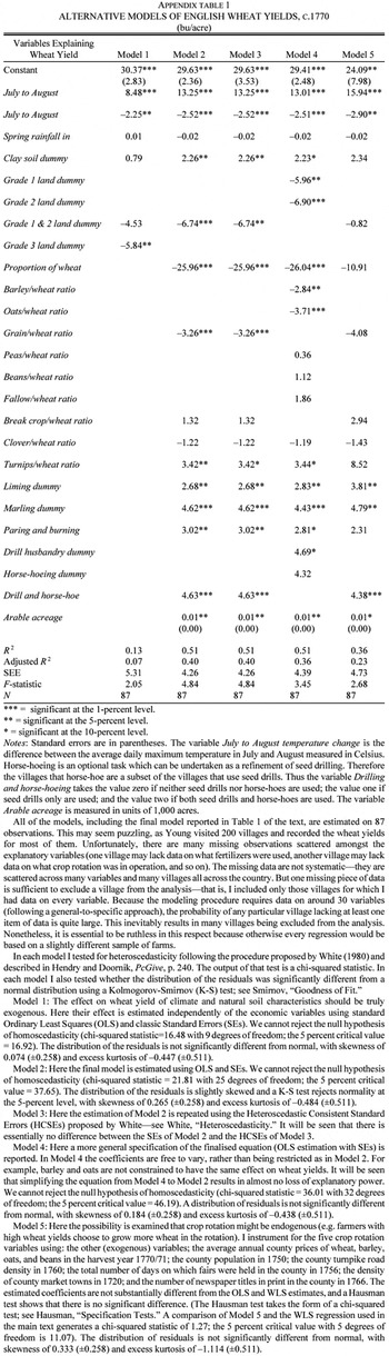
For the sake of clarity I report only the final model in Table 1. This is based on Weighted Least Squares (WLS) estimation because there is some evidence of heteroscedasticity. There was no evidence of measurement error or endogeneity, so I did not persist with Instrumental Variables (IV) estimation, because it is unnecessary and less efficient. A more detailed discussion of these issues and other versions of the model are reported in full in the Appendix. Let us now consider in detail the magnitudes and importance of the coefficients estimated, starting with the role of climate (C1–C4).
The Role of Climate
By far the most important climatic factor determining the wheat yield in Western Europe is rainfall because the grain yield is susceptible to rainfall fluctuations throughout the growth cycle. But the relationship between rainfall and yield is complicated. We are not concerned only with the total quantity of rainfall but also how it is distributed over short periods.33
This article differs in this respect from previous studies of weather and output, such as Solomou, “Climatic Variations,” pp. 53–67. To capture annual weather shocks Solomou uses a variable called Mean Soil Moisture Deficit, which is a complex amalgam of monthly rainfall and temperature based on various assumptions about cropping patterns and other factors. This may be a useful approach to estimating total agricultural output (which comprises a broad range of crops maturing in different months of the year). But we found that it had little explanatory power for wheat yields alone. This is not surprising because aggregation throws away information that might have explanatory power.
The model suggests that three phases of the growth cycle are particularly sensitive to rainfall. The first period is spring (April to June) when the wheat plants are developing; the second period is early summer (July) when the grains are “filling” (that is, becoming mature and plump); and the third period is late summer (August) when the grain is harvested.
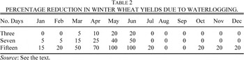
Excessive spring rainfall can reduce yields by water logging the soil and thus interrupting the flow of oxygen to the roots. It can also promote the spread of fungal plant diseases such as “rust,” for which there was no cure in the eighteenth century. The estimated model shows that this was a particular problem in areas with poor drainage. In a normal year the mean Spring Rainfall in Poor Drainage Areas was 135 millimeters, which reduced the local wheat yield by 2.7 bushels (11 percent). This result fits closely with modern experimental data, as Table 2 demonstrates.34
These data are taken from Trafford, “Field Drainage,” pp. 148–49.
Winter wheat is particularly susceptible to water logging in April, May and June (which corresponds to our definition of “spring”), when a three-day period of water logging reduces yields by 10 to 20 percent.
This also enables us to test directly the historical hypothesis that hollow drainage was an important method of raising yields (T4), and shows that the effects were indeed quite large. Hollow draining involved digging trenches across a field and filling the bottom of the trench with a material which permitted the free flow of water (such as stones or clay pipes), before refilling the trenches with earth. This was an expensive technique for removing excess water but the drains normally lasted a long time and the benefits could be felt for 50 years or more. Young noted whether or not a village needed hollow draining and whether or not draining had been undertaken. Spring Rainfall led to a mean yield reduction of 11 percent in Poor Drainage Areas (where drainage was required but not installed). But there was no significant reduction in areas that had been hollow drained.
As the growing season advances into July it is important to have sufficient moisture to allow proper grain filling. This does not mean that heavy rainfall is beneficial; rather, it is useful to have light rain on a large number of days. By contrast, as we move towards the harvest time in August the climate should be as dry as possible because any rainfall is likely to damage the mature crop. Hence the harvest of 1811 (estimated at 40 percent below normal) was very wet and “… one half of the corn was exposed for three weeks to rains and storms, much of which was badly sprouted.”35
Taken from the Farmer's Magazine, quoted in Jones, Seasons, p. 159.
However, in the United Kingdom there is a strong correlation between July and August precipitation (i.e., places which are wet in July also tend to be wet in August), so in effect there is a trade-off between July and August climate. Ideally there would be (light) rainy days in July but none in August, so
July to August Rainy Days Change would be large and negative. In fact, the mean
July-August Rainy Days Change in the sample of villages is −0.34 and the range is 2.00. So the mean wheat yield is 1.0 bushels higher than if July and August had an equal number of rainy days (–0.34 * −2.82=0.96); and the place where July and August rainfall is most conducive to wheat production has an advantage of 5.6 bushels over the place where July and August rainfall is least conducive to wheat production (2.00 * −2.82=−5.64).
The role of July and August temperature in determining wheat yields is more straightforward. For most of the life cycle of the wheat plant there is no relationship between temperature and the future grain yield of the plant: temperature affects only the date at which the wheat plant reaches maturity. (This is leaving aside periods of extreme temperature that are atypical of Britain). But once the wheat plant has matured and started to produce grain then the temperature becomes important. Vos has shown that reducing the temperature from 22 degrees Celsius to 16 degrees Celsius would prolong the period of grain filling by 20 days (50 percent) and lead to an increase in yield of 25 percent.36
Vos, “Modelling,” p. 144.
In Britain most of the grain filling occurs in July, so lower July temperatures are highly desirable (because everywhere in Britain has average July temperatures above 16 degrees Celsius). By contrast, when the period of grain filling has ended high temperatures are extremely useful in drying out the crop to avoid sprouting and other damage. Hence a hot August is very beneficial. Unfortunately, July and August temperatures are highly correlated across Britain and we again see a trade-off between July and August climate–we would like a cool July to improve grain filling but a hot August to improve the harvest. Hence we are really interested in the
July to August Temperature Change and the mean change in the sample of villages is −0.24 and the range is 1.10. So the mean wheat yield is 3.4 bushels lower than if the temperature were the same in July and August (−0.24 * 14.00=3.36); and the place where July and August temperatures are most conducive to wheat production has an advantage of 15.4 bushels over the place where July and August temperatures are least conducive to wheat production (1.10 * 14.00=15.40). The poor harvest of 1808 had all the ingredients of a poor summer suggested by the model. A contemporary noted: “The crops more deficient than last year. The hot days in the early part of July did great injury to the wheat, and they were followed by a great deal of wet and stormy weather, from that time until the getting in of the harvest.”
37 Quoted in Jones, Seasons, p. 158.
The model is therefore consistent with the CERES model with regard to the impact of climate (C1–C4). Rainfall is indeed a crucial determinant of wheat yields from spring onwards; temperature has an important effect on yields (mainly through water availability); and climatic factors become more critical around harvest time. The effect of altitude (C4) also had the expected sign but had little explanatory power.
The Role of Natural Soil Fertility
The model also enables us to quantify the effects of natural soil fertility (S1) and crop rotation. Using Model 4 in the Appendix, I replaced the crop rotation variables with a dummy for Grade 3 land. This enabled me to quantify the differences in yields on all the grades of land. The coefficients on the dummies on Grades 1, 2, and 3 land were −5.7, −7.1, and −8.2 respectively.38
The control group is comprised of farms on Grade 4 land. We would typically expect yields on these farms to be lower than the other grades (rather than higher, as is the case here) because Grade 4 land was generally of low quality and not suitable for arable production. However, in this period there were some attempts by experimental farmers to bring Grade 4 land into arable cultivation, using immense (and probably uneconomic) amounts of capital inputs such as manuring and draining. As a result, in the sample there are a small number of arable farms on Grade 4 land and the yields on these farms were fairly high.
Of course, this is a function of both natural fertility and systematic variation in crop rotation—and it understates the effect of natural fertility because the more fertile soils were farmed more intensively. If the rotation on Grade 3 land were adjusted to be the same as on Grade 2 land then the difference between the dummies would increase from 1.1 to 1.4 bushels per acre. If the Grade 3 rotation were adjusted to be the same as the Grade 1 rotation, then the difference would rise from 2.5 to 4.4 bushels per acre. It is encouraging that soils of different quality are ranked as expected (Grade 1 is best, etc.) and the coefficients are plausible. The historical implications of this result are discussed in the next section.
I also found that wheat yields were 2.5 bushels higher on clay soils. Clay soils have a number of benefits. In particular, they are capable of retaining moisture, humus, and chemical compounds in a kind of “nutrient sink” that is difficult to destroy. Hence it is no surprise to find that they have higher yields.
The Role of Technology
T1, Crop rotation: Controlling for natural soil fertility allows us to test for the effect of crop rotation. Growing more break crops and fewer grain crops improves the fertility of the soil by increasing the stock of nitrogen. Of course, the effect on wheat yields will be larger when the proportion of wheat in the crop rotation is smaller because the stock of nitrogen per wheat plant is higher when there are fewer wheat plants. Hence the explanatory variables are turnip-wheat ratio, clover-wheat ratio, etc. I found that the effect of crop rotation only became apparent when the crop ratios were interacted with dummies to control for the grade of the land. That is, I estimated the effect of variations in crop rotation on Grade 1 land; and then on Grade 2 land independently; etc. This is the correct method of modeling if crop rotation has a different effect on different grades of land, which seems to be borne out by the data. I found that crop rotation was important only on Grade 3 land, probably because manipulating the nitrogen cycle is more critical on land that is less naturally fertile.39
However, we cannot rule out the possibility that crop rotation was also important on other grades of land. We may have failed to get a significant result due to the small sample size. Whereas we have 54 villages on Grade 3 land we have only 29 villages on Grade 1 and 2 land. Remember that estimating the effect of crop rotation involves the estimation of five additional variables.
As the vast majority of agricultural land is Grade 3, the impact of crop rotation is in any case widespread and the results are of considerable empirical importance. The following points are worth highlighting.
As expected, cultivating grain crops (wheat, barley, and oats) reduces the wheat yield. By contrast, break crops (such as beans, peas, and bare fallow) all have a modest positive impact on wheat yields. The role of turnips and clover is particularly interesting because they were only just coming into general use in the eighteenth century and it has been widely argued that they significantly boosted productivity.
T2, Turnips: I find that turnips have a much more positive impact than the other break crops. There are two likely explanations for the strong showing of turnips. First, turnips added a lot of humus to the soil and recycled nitrogen in a more efficient manner than the traditional break crops. So the nitrogen contained in the turnip was made available for subsequent grain production rather than being lost back into the atmosphere. Second, turnip cultivation both required and permitted very strict weed control. Weeds compete with cultivated crops for scarce soil nutrients, so eradicating or suppressing weeds could have a large effect on subsequent grain yields. This argument seems particularly persuasive in the light of the results on seed drilling, which are discussed below.
T3, Clover: The impact of clover in the rotation is more surprising. Theoretical calculations suggest that clover should substantially increase the output of a mixed farm.40
Shiel, “Soil,” pp. 74–75.
The standard argument in the literature is that clover fixes atmospheric nitrogen directly into the soil, in addition to creating animal fodder and (hence) manure. This process should substantially increase wheat yields. The effect should be particularly marked because it was normal for wheat to follow clover immediately in the crop rotation, so there should be few nitrogen losses due to extraneous factors. The quantity of nitrogen available should also have been boosted by the fact that it was normal to grow clover in a field for several years before returning it to wheat production.
In fact, clover has a negative impact on wheat yields. This surprising result is supported by three further pieces of evidence. First, we have analyzed the Young data set using a completely different approach and we still get a negative estimate of the effect of clover.41
Second, we can consider the crop rotation experiments carried out at the Rothamsted experimental farm in the nineteenth century. They show that the effect of clover on subsequent wheat yields is
negative when there are low levels of fertilizer inputs and low yields of clover.
42 Hall, Rothamsted, p. 200.
This is because the clover plants require a substantial amount of nitrogen to get themselves established before they can start putting nitrogen back into the soil, so if they do not manage to get well-established then their overall effect on the nitrogen balance can be negative. A clover yield of 15.2 cwt at Rothamsted was associated with a
decline in wheat yields of 16.7 percent, whereas a clover yield of 44.4 cwt was associated with a wheat yield
increase of 7 percent. If we interpolate linearly between these points, then the mean clover yield of 33.3 cwt observed in the Young sample would be associated with a wheat yield reduction of 2 percent (0.5 bushels per acre). This compares to an estimated negative effect of 1.5 bushels in the model. Third, clover was typically harvested and used as hay for winter fodder. The dung thus created during the winter was stored until spring, when it was returned the field during spring muck-spreading. Most of the nitrogen in the manure was probably lost back into the atmosphere during the winter. We know that even under ideal conditions it is normal to lose 50 percent of the nitrogen content of stored manure.
43 Voelker, “Manures,” pp. 610–18.
So making clover hay could easily lead to a net
reduction in the amount of nitrogen available for grain crops (and hence lower yields).
Ideally, we need to assess the magnitude of the coefficients in the model (not just whether or not they have the right sign). One test of the model is to simulate different crop rotations and compare the predictions to data from experimental farms. Table 3 shows the estimates of the effect of continuous wheat cultivation, a “medieval” rotation of wheat-fallow, and a “modern” four-course rotation. The yield levels and the differences between the rotations are similar in the simulations and the experiments. Note that the estimate for continuous wheat is less accurate than the other estimates because the predictions are much further out-of-sample (no one in the data set grows anything like 100 percent wheat, so the regression coefficient is less appropriate for that simulation).
T5, Mixed farming: The eighteenth century is said to have seen a move towards more mixed farms (i.e., farms containing both arable and livestock in substantial proportions); the new root crops that replaced bare fallow were used to feed animals and the resulting dung was used to fertilize the arable crops.44
Shiel, “Soil,” pp. 67–70.
Some researchers have even suggested that in England: “…the availability of organic fertilizer [dung] exercised a decisive influence on the level of physical yields achieved in the cultivation of cereal, potatoes and other crops.”
45 O'Brien and Keyder, Economic Growth, p. 137.
I tested for this effect directly by estimating the amount of dung produced in the village (as a function of the horses, oxen, cattle, and sheep available) and then entering this variable into the model of wheat yields. I also tested indirectly for the effect of mixed farming by just entering the arable-pastoral ratio as an explanatory variable. In neither case could I find any effect on wheat yields from mixed farming. Interacting each of the variables with the grade of land made no difference to the results.
T6, Manuring techniques: In general, it is not surprising that there is no simple relationship between mixed farming and higher yields: as noted previously, the quantity of manure produced from a given quantity of fodder depends strongly on the techniques employed. One might ask why mixed farming became more popular if it offered few benefits for arable yields. But it should be noted that mixed farming could have been very important in raising total agricultural output, even if arable yields were depressed, because it may have substantially increased meat output. I am simply arguing here that mixed farming had no detectable effect on wheat yields.
T7, Liming and Marling: Let us turn to the question of liming and marling. Most soil is naturally acidic and it becomes more acidic when crops are cultivated. This is because many alkaline compounds are broken down when chemicals are removed from the soil to furnish nitrogen, phosphorus, and potassium for healthy plant growth. Although most crops prefer a slightly acidic soil, their tolerance of acidity is quite low and in the face of continued cultivation the soil naturally becomes too acidic for them.46
Donahue et al., Soils, p. 246.
Turnips are particularly averse to acidic soils, so the issue of acidity became even more important with the diffusion of turnips during the eighteenth century. The most common way to correct soil acidity was to add either lime or marl to the soil. These are both forms of calcium carbonate (which is alkaline) that occur naturally in different regions of England; after simple preparation they can be spread on the acidic farm land and mixed in with a plough. Marling was particularly popular after 1750 because the cost of labor was relatively low and marling is very labor-intensive.
47 Dodgshon, “Land Improvement,” p. 2.
The positive effect of marling and liming is generally thought to have been large, and indeed Young called marl “the Prince of Manures.”
48 In the eighteenth century the word “manure” had the same meaning as “fertilizer.” See Young, Farmer's Kalender; or “Manure” in the Oxford English Dictionary.
The model suggests that liming increased output by 2.7 bushels (11 percent) and marling increased yields by 5.4 bushels (22 percent). I tried testing for the effect of other types of manure, such as ashes and pigeon dung, but the number of adopters of each type was too small to give any reliable results. By contrast, 48 percent of the sample used lime and 17 percent used marl.
49 For a detailed analysis of fertilizer use, see Brunt, “Where there's Muck.”
T8, Seed: It seems reasonable to expect higher volumes of seed sown to result in higher yields. But in fact the sign on seed volume was negative and statistically insignificant. There are three possible explanations for this. First, it may be the case that there were variations in the variety or quality of seed employed, so that farmers using low-quality seed may have used more seed and still obtained lower yields. If this hypothesis were true then we might expect to see a marked regional pattern because all farmers buying their seed from the same source would face the same problem. However, regional dummies did not improve the fit and therefore this seems to be an unlikely explanation (although it is the subject of on-going research). Second, some areas may have been more prone to weeds than others. One (partial) solution to the weed problem was to sow more seed and try to choke out some of the weeds. This could cause the apparent correlation of plentiful seed and low yields. Third, there is some evidence that it was possible to use too much seed. The growth of wheat plants was constrained by the quantity of nutrients available (especially nitrogen). If seed were sown intensively and a high proportion germinated then the wheat plants would effectively be competing with each other for nutrients; all of the plants might continue to grow until the nutrients were exhausted and then all the plants would give a very poor yield. A later farmer noted that: “… I find it imperative to sow thin, say 3 to 4 pecks per acre, or the crop would be mostly straw.”50
Mechi, “Thin Sowing,” pp. 537–39.
Hence we might not expect to find the positive relationship between seed rates and yields that we observe today.
T9, Ploughing: We would normally expect more ploughings to raise the yield of any crop. This would explain why more valuable crops received more ploughings: four for wheat; three for barley; two for turnips; and one for oats, peas, and beans.51
All data taken from Young's Tours, using only those places for which we have all the data (so that it is based on a constant and uniform sample).
In fact, the sign on the number of wheat ploughings was perverse and insignificant. There are two possible explanations for this result. First, plough design varied enormously across the country and it may be the case that less effective ploughs induced more cultivations but lower yields. I tested for this in several ways, such as using a dummy variable to reflect whether or not wheel ploughs were being used. Although the evidence cannot be conclusive (because we do not have a perfect measure of plough effectiveness) I think that it is unlikely that variations in plough-type are driving this result. Second, it is certainly true that some soils require more ploughing than others but still give lower yields. I tried interacting plough type and soil type without success, but it is possible that this aspect of soil type has been captured only imperfectly in the soil variables.
T10, Drilling and horse-hoeing: An important hypothesis to be tested was whether drill husbandry and horse-hoeing raised yields. Drilling seed into the ground instead of sowing it broadcast allowed farmers to control weeds much more effectively. Before the invention of herbicides in the twentieth century weeds were very problematic because they were impossible to eradicate on a permanent basis (they reproduced rapidly and often ran deep into the soil). The detrimental effect on yields arose from the fact that weeds competed very effectively for the limited amounts of nitrogen that were available for plant growth. The traditional method was to sow seeds broadcast and wait until the spring (when the wheat plants were just shooting) and then harrow out any weeds which had started to grow.52
A harrow is like a large rake: it has a framework of spikes that dig vertically into the ground. When the harrow is dragged over the crop the wheat shoots (which grow vertically) are left largely unscathed but the weeds (which are larger and often grow horizontally) are ripped out.
But harrowing was not very effective because many weeds survived and many others had yet to start growing.
53 Brenchley, “Weeds,” pp. 14–37.
By contrast, drilled seed was planted in straight rows and it was then possible to weed between the rows with a hoe and attack the weeds much more effectively and much later in the season. Hoeing could either be done by hand or with a horse-hoe.
54 The celebrated proponent of horse-hoeing is, of course, Jethro Tull. See Tull, Husbandry.
The model shows that both seed-drilling and horse-hoeing were important innovations, each raising yields by 5.2 bushels.
T11, Farm size: The issue of wheat yields and farm size has featured prominently in the literature on enclosure. The agricultural improvers of the eighteenth century were adamant that the creation of large farms through enclosure led to greater efficiency. But they also maintained that large farms employed relatively more labor than small farms (so the efficiency gains cannot have been due to cost-cutting). In order for these claims to be compatible it would have to be the case that yields were higher on large farms. On the basis of a casual examination of the Young data set, Allen has argued that yields were not higher on large farms, so the benefits of enclosure must have been felt through labor-cutting.55
Allen, Enclosure, p. 202.
I tested whether or not yields were higher on large farms taking into account the impact of all the other factors (soil, etc.). The model shows that wheat yields were definitely higher on large farms but the effect was small. An increase in farm size from 100 to 200 acres was associated with wheat yields that were higher by 0.5 bushels per acre (2 percent).
Whilst this finding on farm size has some interesting implications for the enclosure debate, we should be wary of drawing any conclusions about economies of scale more generally because it is not obvious why there should be any economies of scale in eighteenth century wheat production. It is likely that large farms found it more economic to make capital investments that covered large geographical areas. For example, drainage projects suffered from a free-rider problem that inhibited installation and maintenance in areas where the ownership of land was divided. But the effect of this on yields should already be captured directly by the drainage variable. Moreover, there could be other explanations for the correlation between farm size and wheat yields. In particular, it could be the case that good farmers have higher yields and over time they migrate towards larger farms. This would not be a true economy of scale, merely an unmeasured input (the superior skill of the farmer). Further work needs to be done on this in order to reach a definitive answer.
DISCUSSION
Overall the model suggests that traditional characterizations of the Agricultural Revolution have focused on the wrong techniques when trying to explain increases in productivity. Contrary to popular belief, the move to mixed farming contributed little to arable production; the introduction of clover was not associated with higher wheat yields; and there is no evidence that more frequent ploughing had a positive impact.
There were only two eighteenth-century innovations that had a substantial impact on yields. First, there is the turnip, which improved soil quality by adding humus and reducing the competition from weeds. Second, the model shows that the other really important technological innovation in the eighteenth century was seed-drilling—a technique that has generally been dismissed in the literature as unworkable and uneconomic. In fact, evidence presented in the next section suggests that the diffusion of drilling was a primary factor pushing up yields between 1750 and 1850.
The two other techniques that had an important impact on wheat yields in the Agricultural Revolution were not at all novel. First, adding alkali by liming or marling had been known for many years.56
Mathew, “Marling,” p. 104.
The striking effect of liming and marling would come as no surprise to a modern arable farmer, for whom the first task is correcting soil acidity. Even other forms of fertilization (for example, adding nitrogen) are a secondary concern. Second, hollow drainage was not a new technique, it was just very expensive. The massive increase in drainage schemes in the nineteenth century (particularly after cheap tile piping had been invented) was undoubtedly another cause of higher yields. Draining, liming, and marling are distinguished by being very capital and labor intensive. Their increasing popularity in the late eighteenth century was probably due to a combination of a rising wheat price, a falling real wage, and a falling interest rate.
Having established the role of climate, soil, and technology in raising English wheat yields we can now explore more fully the implications of this new information. In the next section we undertake some counterfactual simulations to test the sensitivity of wheat yields to changes in environment and technology.
THE AGRICULTURAL REVOLUTION IN DIFFERENT STATES OF NATURE
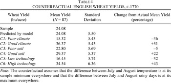
This section begins by testing the sensitivity of the model to changes in the values of different variables. In particular the power of environmental factors (climate and soil quality) are compared to technological factors (crop rotation, seed drills, and so on). In Table 4 presents six counterfactual scenarios.
We would expect the climate to be the single most important factor determining wheat yields in the eighteenth century—even in England, which had the most advanced agricultural system in the world. The climate counterfactuals (C1 and C2) do indeed demonstrate the dominant role of climate in determining yields, and show that average yields in England would have been 51 percent higher if everywhere in England had enjoyed the climate of the place most suited to wheat production. This also gives some idea of the potential benefits to be gained from increased regional specialization in agriculture in the nineteenth century.
The soil-quality counterfactuals show that variations in the natural fertility of the soil had only a modest impact on wheat yields (C3 and C4). Reducing soil quality to Grade 3 would have reduced the average yield by only 5 percent, whereas leveling soil quality up to Grade 1 would have raised average yields by 22 percent. This is simply because the vast majority of villages (62 percent) had Grade 3 land; 24 percent had Grade 2 land and only 9 percent had Grade 1 land.
As noted previously, English agricultural productivity was exceptionally high by international standards. O'Brien and Keyder argue that England's natural endowment was largely responsible for her superior productivity, stating that: “Furthermore, the quality of land available to British farmers was hectare for hectare definitely superior to the quality of French farmland…. [So] differences in the quantity and quality of land account for most of the gap in the productivity of labour employed in British and French agriculture …”57
O'Brien and Keyder, Economic Growth, pp. 112–13.
The results here cast serious doubt on the O'Brien and Keyder thesis. If we gave everyone in England low quality land then the England-France yield gap could not have fallen by more than 1.3 bushels. Moreover, this is an upper bound on the size of the land-quality effect because it implicitly assumes that everyone in France had low quality land. For a fair comparison we ought to revise downwards French yields as if everyone in France were also using low quality land. Because French yields were around 13.3 bushels in 1789, the yield gap was 10.7 bushels per acre—so differences in land quality cannot explain much (if any) of England's advantage.
58 Allen and O'Grada, “On the Road Again,” pp. 108–15 and table 4.
The influence of man-made factors (which we have loosely termed “technology”) was far greater than soil quality (C5 and C6). It is the take-up of technology that explains England's productivity advantage over France. The French grew a much higher proportion of grains in their crop rotation and no turnips. This had the effect of driving their wheat yields 5.7 bushels below the level of English yields, explaining much of the productivity difference in 1770.59
The percentage distribution of crops c.1770 in England/France was: wheat 19/10; barley 18/8; oats 17/23; rye 0/19; (total grains 54/60); peas 9/3; beans 3/2; turnips 12/0; clover 10/0; fallow 12/34. English data are taken from Young, Tours (the detailed minutes for each farm), and French data from Toutain, “Produit,” pp. 48–76, 91–92.
The high-technology counterfactual also shows that if everyone had adopted the most productive technologies available in 1770, then English yields could have been 43 percent higher than those actually observed by Arthur Young. This casts doubt on the argument that England would have developed along similar lines to Ireland, in the absence of an Industrial Revolution. The argument runs that the lack of industrial exports would have removed England's ability to import grain in the late eighteenth century and led to a redistribution of land and labor resources in favor of more nutritious (but labor-intensive) food products—namely, potatoes. Hence England would have followed the Irish route and become ever more specialized in agriculture. In fact, the model suggests instead that rising wheat prices in England would probably have led to faster adoption of new technology (such as seed drills) and increased wheat production. If there had been no increase in wheat land but all farmers had used the most productive technology available in 1770, then English agriculture could have fed the English population of 1810.
We can decompose the postulated yield increase (C6) to find the potential for each technique to raise output after 1770. Such a decomposition shows that seed drilling and horse-hoeing were the most important by far (78 percent of the postulated increase). Adopting the Norfolk four-course crop rotation was second in importance (20 percent of the postulated increase). Other innovations were small by comparison, such as under-drainage (2 percent of the postulated increase). These estimates of the returns to various technologies may seem surprising. In particular, the prominence of seed-drills in the model runs contrary to the received wisdom of technological change in the Agricultural Revolution. But seed drills and horse-hoeing together had a massive potential to raise average yields because they had a large impact on yields (10.4 bushels per acre) and enormous scope for further adoption (from 8 percent to 100 percent). There was a sustained growth in the adoption of seed drills after 1810, and by 1880, 60 percent of farms were using a seed drill.60
Walton, “Mechanisation,” pp. 23–42.
By contrast, the potential for under-draining to raise yields was quite small because only a limited number of villages could benefit from better drainage.
CONCLUSIONS
The model presented in this article substantially improves our understanding of wheat production in the eighteenth century. For the first time it draws together all the environmental and technological factors that determine the output of wheat and estimates their impact simultaneously. The model offers important new insights into both the level and growth of English wheat yields during the Industrial Revolution.
English yields were substantially higher than those achieved in other European countries during the Industrial Revolution. The counterfactuals show that climate had the largest influence on yields and English farmers would have benefited greatly from a more benign climate. The endowment of soil quality in England was also mediocre for the most part and cannot explain much (if any) of England's yield advantage. In fact, the English productivity advantage over France in 1770 was due largely to superior technology, such as turnips and seed drills. This is scarcely surprising, given the widespread interest in agriculture amongst Englishmen of all classes and the higher levels of capital investment.61
Hickey, “Innovation,” pp. 208–30.
Technological improvement and increased investment also explain the growth in English yields over time. The model shows that turnips, drilling, and marling were most effective in raising yields. Turnips diffused rapidly after 1700 and were already fully diffused by 1770 (there was virtually no increase in the proportion of turnips in the crop rotation between 1770 and 1870).62
Ministry of Agriculture, Agricultural Statistics.
By contrast, drilling became important only after 1810 and thereafter became steadily more important until 1880.
63 Walton, “Mechanisation,” pp. 23–42.
There is much less information available on the extent of marling. Marling was a very old technology known in medieval times and there was no diffusion as such occurring during the Agricultural Revolution. But changes in relative prices (the high price of wheat and the low price of labor) made marling increasingly popular after 1700. Thus turnips, drilling, and marling were probably the primary causes of increasing wheat yields between 1700 and 1850.
I began the analysis by outlining the important role of agriculture in facilitating the English Industrial Revolution. In the eighteenth century, high agricultural labor productivity was a prerequisite for workers to be released to the new factories and cities. In this article I have shown that the new technologies coming into use after 1700 were important in raising agricultural productivity. Hence it was not an accident that England had exceptionally high productivity by international standards—and it was not by chance that the Industrial Revolution occurred in England.
Appendix: Alternative Models of English Wheat Yields
This appendix includes alternative specifications of the model. This is important because it demonstrates that the results are robust to potential data and estimation problems. Notice, in particular, that the observed values for each village are actually estimates made by Young on the basis of his survey of a sample of farms within the village. This can create measurement error in the data. For example, we do not know the true value of the average yield in each village; instead we have an estimate of the average yield in the village based on the yields reaped on the farms that Young happened to visit. Therefore the average yield in the village as recorded by Young may deviate randomly from the true yield. This can generate two problems. If the errors occur in the yield data, then the regression may suffer from heteroscedasticity. If the errors occur in the other variables, then the coefficients that we estimate will be biased downwards. Let me make these points in the context of the econometric model.
I denote Young's estimate of the village yield as yvf. What we observe in the data is therefore
where ef is a random error with mean zero. Young visited many more farms in some villages than in others (a minimum of one and a maximum of nine) and one might well expect this to affect the variance of ef—thus creating heteroscedasticity in the errors that affects the efficiency of the estimating procedure. I test and control for this possibility in the empirical analysis using the various procedures proposed by White and also Weighted Least Squares (WLS).
64 White, “Heteroscedasticity.”
The heteroscedasticity problem proves to be mild. I estimated the model by OLS (Model 2 in Appendix Table 1) and tested the residuals using the techniques proposed by White and Glejser.
65 White, “Heteroscedasticity”; and Glejser, “Heteroscedasticity.”
There is a positive relationship between the variance of the residuals and the number of farms visited in the village, although it is only significant at the 7-percent level.
where Rv is the absolute value of the residual for each village v; Fv is the number of farms in the village; and standard errors (SEs) are in brackets.
I investigated the issue further and in Model 3 I report White's Heteroscedastic-Consistent Standard Errors (HCSEs). It will be seen that there is essentially no difference between the HCSEs of Model 3 and the classic SEs of Model 2. Using WLS to control for potential heteroscedasticity reinforces this conclusion. A comparison of Model 2 (OLS) with Table 1 (WLS) shows that neither the estimated coefficients nor the standard errors are sensitive to alternative estimation procedures. Nonetheless, if there is any evidence of heteroscedasticity then it makes sense to persist with the WLS estimates. WLS will give somewhat more precise results because it uses all of the available information. Hence I frame the discussion in terms of the WLS equation reported in Table 1.
A more serious problem arises from the possibility that measurement error could be present in the exogenous variables, which would bias downwards the estimated coefficients. There is unlikely to be any problem with the climate and soil variables because they are measured very precisely using modern scientific instruments and trained technicians (although I also tested for this type of measurement error). But the technology variables, such as crop rotation, are again estimates by Young based on his sample of farms. That is
where vkf is a random error with mean zero. Then we have
If the term Σkτkvkf>0 then the estimated coefficients will be biased downwards. I obviously need to test and control for this possibility, and I do so by employing Instrumental Variables (IV) techniques and a Hausman test.
66 Hausman, “Specification Tests.”
In fact, one can firmly reject the hypotheses of measurement error and endogeneity in the crop rotation variables. I instrumented for crop rotation using the (other) exogenous variables, product prices, and several additional demand-side variables such as local population and road density. These variables are correlated with the crop rotation variables but are unlikely to be correlated with the errors. We can see from Model 5 that instrumenting for crop rotation has very little effect on the model and a Hausman test overwhelmingly rejects the hypothesis of mis-specification.
I do not find the IV results to be particularly surprising. Farmers optimize their rotation on the basis of local growing conditions and local prices. This minimizes the problems of both measurement error and endogeneity. First, because growing conditions and prices do not vary much within the village, it tends to be the case that all the farmers in the village grow the same crop rotation. So the measurement error vkf that arises from sampling a sub-set of farms is likely to be small. Second, local prices vary considerably across villages. So it may be the case that the level of wheat yields will (partially) determine the percentage of land devoted to wheat. But when we look at a cross-section of villages this effect is likely to be swamped by the influence of variations in local prices.67
Notice also that the crop rotation is determined by relative prices and yields. Suppose that there is a positive shock to wheat yields in the village. This will only result in a change in the crop rotation (that is, more wheat being grown) if the yields of other crops are left unchanged by the shock. In reality it seems likely that a shock which impacts positively on wheat yields will also impact positively on the yields of the other crops. Hence there is unlikely to be much effect on crop rotation.
This research was funded by the Economic and Social Research Council and the Fulbright Commission. I am grateful to the Harvard economics department for hosting me whilst I was working on this article. I would like to thank Edmund Cannon, James Foreman-Peck, Oliver Grant, Felix Ng, Avner Offer, Adrian Pagan, and especially Lucy White for helpful comments. Any remaining errors are my own responsibility.