1. Introduction
Turbulent flows in rotating reference frames are of great importance in astrophysical, geophysical and engineering applications. Flow in a turbomachine rotor is a typical example, where both the mean flow and the turbulent structures will be greatly affected by the system rotation (Johnston Reference Johnston1998). A great deal of effort has been devoted to investigating the effect of system rotation on turbulence. In this paper, we focus our attention on turbulent channel flows with spanwise rotation, where the channel rotates around an axis pointing in the spanwise direction with a constant angular velocity.
Investigation of the effect of spanwise rotation on fully developed turbulent channel flows has a long history. Johnston, Halleen & Lezius (Reference Johnston, Halleen and Lezius1972) conducted an experimental study of the problem, and three stability-related phenomena were observed, including reduction (increase) of the rate of wall-layer streak bursting in locally stabilized (destabilized) wall layers, total suppression of transition to turbulence in a stabilized layer and the development of large-scale roll cells on the destabilized side of the channel. Besides exposing the change of some underlying structures caused by rotation, they provided plenty of quantitative data, including the
 $2{\it\Omega}^{\ast }$
-slope of the mean velocity profile near the pressure (unstable) side (
 ${\it\Omega}^{\ast }$
is the angular velocity). Experimental studies have also been performed by, e.g., Nakabayashi & Kitoh (Reference Nakabayashi and Kitoh1996), Maciel et al. (Reference Maciel, Picard, Yan and Dumas2003) and Nakabayashi & Kitoh (Reference Nakabayashi and Kitoh2005). Nakabayashi & Kitoh (Reference Nakabayashi and Kitoh2005) investigated the turbulence characteristics, including turbulence intensities, Reynolds shear stress, correlation coefficient, skewness and flatness factors, four-quadrant analysis, autocorrelation coefficient and power spectra, by using their experimental data.
Thanks to the rapid development of computer science and numerical technology, numerical approaches have become prevalent tools to investigate turbulence. Tafti & Vanka (Reference Tafti and Vanka1990) investigated the effects of spanwise rotation on the large-scale structures in turbulent channel flow using large eddy simulation (LES) with the Smagorinsky model at a friction Reynolds number of
 $Re_{{\it\tau}}=u_{{\it\tau}}^{\ast }h^{\ast }/{\it\nu}^{\ast }=180$
(
 $u_{{\it\tau}}^{\ast }$
is the friction velocity,
 $h^{\ast }$
is the channel half-width and
 ${\it\nu}^{\ast }$
is the kinematic viscosity). Their simulation results were shown to be consistent with previous flow visualization data and measurements, and they found that the roll cells made a significant contribution to the total turbulent quantities. Kristoffersen & Andersson (Reference Kristoffersen and Andersson1993) performed the first direct numerical simulation (DNS) on a spanwise-rotation channel at
 $Re_{b}=U_{b}^{\ast }h^{\ast }/{\it\nu}^{\ast }\approx 2900$
(
 $U_{b}^{\ast }$
is the mean bulk velocity). The rotation number
 $Ro=2{\it\Omega}^{\ast }h^{\ast }/U_{b}^{\ast }$
varied from 0 to 0.5. Their results showed that the augmentation and suppression of turbulence along the pressure (unstable) and suction (stable) sides respectively become more significant with increasing rotation for
 $0\leqslant Ro\leqslant 0.5$
, resulting in highly asymmetric profiles of mean velocity and turbulent Reynolds stresses. The
 $2{\it\Omega}^{\ast }$
-slope of the mean velocity profile was also reported, together with the vanishing Reynolds shear stress in the vicinity of the stabilized side at
 $Ro=0.5$
. Lamballais, Lesieur & Métais (Reference Lamballais, Lesieur and Métais1996) studied the structure of the instantaneous vorticity field in both transitional and turbulent channel flow with spanwise rotation by means of DNS. They found that the vortex topology is strongly affected by rotation. Alvelius (Reference Alvelius1999) conducted DNS of spanwise-rotation channel flows at
 $Re_{{\it\tau}}=180$
and 360 using different computational domains. It was concluded that the box-length requirement is stricter for low rotation numbers than for higher rotation numbers due to the very elongated structures occurring at lower rotation numbers. Grundestam, Wallin & Johansson (Reference Grundestam, Wallin and Johansson2008a
) investigated the spanwise-rotation channel flow at different rotation numbers through DNS. They focused on higher-rotation-number cases and found that the flow will become completely laminar at
 $Ro\leqslant 3.0$
. Recently, Yang & Wu (Reference Yang and Wu2012) studied the channel turbulence with spanwise rotation for
 $0.00639\leqslant Ro\leqslant 1.318$
by using DNS and helical wave decomposition. They reported that the fluctuation energy is concentrated into large-scale modes for slow rotation, while the concentration shifts towards smaller scales as the rotation rate increases. An inverse energy cascade was also reported in the strong-rotation case.
Since the profiles of mean velocity and Reynolds shear stress are highly asymmetric, channel flow with spanwise rotation represents a challenge for both Reynolds-averaged Navier–Stokes (RANS) and LES models (Jakirlić, Hanjalić & Tropea Reference Jakirlić, Hanjalić and Tropea2000), which makes it a popular test case for both the RANS and LES communities. Piomelli & Liu (Reference Piomelli and Liu1994), Lamballais, Métais & Lesieur (Reference Lamballais, Métais and Lesieur1998), Liu, Lu & Zhuang (Reference Liu, Lu and Zhuang2004), Marstorp et al. (Reference Marstorp, Brethouwer, Grundestam and Johansson2009) and Yang et al. (Reference Yang, Cui, Zhang and Xu2012) used this problem to test the capability of their subgrid-scale (SGS) stress models, while Launder, Tselepidakis & Younis (Reference Launder, Tselepidakis and Younis1987), Jakirlić et al. (Reference Jakirlić, Hanjalić and Tropea2000), Hamba (Reference Hamba2006), Grundestam, Wallin & Johansson (Reference Grundestam, Wallin and Johansson2008b ) and Huang, Ma & Xu (Reference Huang, Ma and Xu2008) employed it to assess their RANS models.
In this paper, DNS of pressure-driven channel flow with spanwise rotation at
 $Re_{{\it\tau}}=180$
are carried out. Differently from previous studies, the global-friction-velocity-based rotation number
 $Ro_{{\it\tau}}=2{\it\Omega}^{\ast }h^{\ast }/u_{{\it\tau}}^{\ast }$
(
 $u_{{\it\tau}}^{\ast }$
is the global friction velocity) here covers a wider range, from 0 to 130. Our focus is on the characteristics of the mean statistics, including the mean velocity, the root-mean-square (r.m.s.) value of the streamwise velocity fluctuations, the Reynolds shear stress, the production term of
 $\langle u^{\prime }u^{\prime }\rangle$
and the turbulent kinetic energy, which were partially studied in the past by Johnston et al. (Reference Johnston, Halleen and Lezius1972), Kristoffersen & Andersson (Reference Kristoffersen and Andersson1993), Grundestam et al. (Reference Grundestam, Wallin and Johansson2008a
) and Yang & Wu (Reference Yang and Wu2012). Our results are consistent with the observations by Grundestam et al. (Reference Grundestam, Wallin and Johansson2008a
) and Yang & Wu (Reference Yang and Wu2012) on the variation of the mean bulk velocity and the local friction velocity at both walls as
 $Ro_{{\it\tau}}$
increases. Specifically, we show several new quantitative results for the r.m.s. value of the streamwise velocity fluctuations, the Reynolds shear stress, the production term of
 $\langle u^{\prime }u^{\prime }\rangle$
and the mean velocity profiles for the first time. These quantitative results will provide new information for researchers who intend to develop or assess RANS and/or LES models for problems subjected to system rotation.
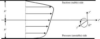
Sketch of the geometry and mean flow of the channel with spanwise rotation.

2. Governing equations and numerical description
Figure 1 is a sketch of the geometry and mean flow of the channel with spanwise rotation. The governing equations for this problem are
 $$\begin{eqnarray}\displaystyle & \displaystyle \frac{\partial u_{i}}{\partial x_{i}}=0, & \displaystyle\end{eqnarray}$$
 $$\begin{eqnarray}\displaystyle & \displaystyle \frac{\partial u_{i}}{\partial t}+u_{j}\frac{\partial u_{i}}{\partial x_{j}}=-\frac{\partial p}{\partial x_{i}}+\frac{1}{Re_{{\it\tau}}}\frac{\partial ^{2}u_{i}}{\partial x_{j}\partial x_{j}}+{\it\varepsilon}_{ij3}Ro_{{\it\tau}}u_{j}. & \displaystyle\end{eqnarray}$$
Here, the Navier–Stokes equations (NS) are non-dimensionalized by the reference velocity
 $u_{{\it\tau}}^{\ast }$
and length scale
 $h^{\ast }$
, where
 $h^{\ast }$
is the channel half-width, and
 $Ro_{{\it\tau}}=2{\it\Omega}^{\ast }h^{\ast }/u_{{\it\tau}}^{\ast }$
is the dimensionless rotation number, with
 ${\it\Omega}^{\ast }$
the dimensional angular velocity. In the following, asterisks denote dimensional quantities unless otherwise stated,
 $(x,y,z)$
or
 $(x_{1},x_{2},x_{3})$
denote coordinates in the streamwise, wall-normal and spanwise directions respectively and
 $(u,v,w)$
or
 $(u_{1},u_{2},u_{3})$
are the corresponding velocity components. The region near
 $y=y^{\ast }/h^{\ast }=-1$
is referred to as the pressure (unstable) side since the background vorticity and the mean shear vorticity have opposite signs, whereas the region at
 $y=1$
is referred to as the suction (stable) side. In (2.2), the centrifugal force has been absorbed in the effective pressure
 $p=P/{\it\rho}+p^{\prime }/{\it\rho}-Ro_{{\it\tau}}^{2}r^{2}/8$
, where
 $p^{\prime }$
is the pressure fluctuation,
 ${\it\rho}$
is the constant density and
 $r$
is the dimensionless distance from the axis of rotation. Here,
 $P$
is the mean pressure and in this study we impose a constant streamwise gradient
 $\text{d}P/\text{d}x=-1$
to drive the flow. The reference velocity
 $u_{{\it\tau}}^{\ast }$
can then be defined as
 $$\begin{eqnarray}\displaystyle u_{{\it\tau}}^{\ast }=\sqrt{-\frac{h^{\ast }}{{\it\rho}^{\ast }}\frac{\text{d}P^{\ast }}{\text{d}x^{\ast }}}. & & \displaystyle\end{eqnarray}$$
The flow can be treated as homogeneous in the
 $x$
and
 $z$
directions, and the mean streamwise velocity component
 $U=U(y)=\langle u\rangle$
(
 $V=W=0$
,
 $V$
and
 $W$
are the mean velocity components in the wall-normal and spanwise directions) is governed by the spatially and temporally averaged Navier–Stokes equations as
 $$\begin{eqnarray}\displaystyle \frac{\text{d}\langle uv\rangle }{\text{d}y}=-\frac{\text{d}P}{\text{d}x}+\frac{1}{Re_{{\it\tau}}}\frac{\text{d}^{2}U}{\text{d}y^{2}}=1+\frac{1}{Re_{{\it\tau}}}\frac{\text{d}^{2}U}{\text{d}y^{2}}, & & \displaystyle\end{eqnarray}$$
where
 $\langle \cdot \rangle$
denotes quantities that are averaged in the
 $x$
and
 $z$
directions as well as in time. In the following, we use a prime to denote the fluctuation components, for example
 $u^{\prime }=u-\langle u\rangle =u-U$
. The three diagonal components of the Reynolds stress tensor and the Reynolds shear stress are
 $\langle u^{\prime }u^{\prime }\rangle$
,
 $\langle v^{\prime }v^{\prime }\rangle$
,
 $\langle w^{\prime }w^{\prime }\rangle$
and
 $\langle u^{\prime }v^{\prime }\rangle$
respectively. Since
 $V=0$
, we can easily obtain that
 $\langle u^{\prime }v^{\prime }\rangle =\langle uv\rangle$
. The turbulent kinetic energy
 $k$
is
 $$\begin{eqnarray}\displaystyle k(y)={\textstyle \frac{1}{2}}(\langle u^{\prime }u^{\prime }\rangle +\langle v^{\prime }v^{\prime }\rangle +\langle w^{\prime }w^{\prime }\rangle ). & & \displaystyle\end{eqnarray}$$
The normalized bulk mean velocity
 $U_{b}$
and volume-averaged turbulent kinetic energy
 $k_{m}$
are defined as
 $$\begin{eqnarray}\displaystyle U_{b}=\frac{1}{2}\int _{-1}^{1}U(y)\,\text{d}y & & \displaystyle\end{eqnarray}$$
and
 $$\begin{eqnarray}\displaystyle k_{m}=\frac{1}{2}\int _{-1}^{1}k(y)\,\text{d}y & & \displaystyle\end{eqnarray}$$
respectively.
Following Kristoffersen & Andersson (Reference Kristoffersen and Andersson1993), we define
 $$\begin{eqnarray}\displaystyle & \displaystyle (u_{{\it\tau}p}^{\ast })^{2}=(u_{{\it\tau}}^{\ast })^{2}\left.\frac{1}{Re_{{\it\tau}}}\frac{\text{d}U}{\text{d}y}\right|_{y=-1}, & \displaystyle\end{eqnarray}$$
 $$\begin{eqnarray}\displaystyle & \displaystyle (u_{{\it\tau}s}^{\ast })^{2}=-(u_{{\it\tau}}^{\ast })^{2}\left.\frac{1}{Re_{{\it\tau}}}\frac{\text{d}U}{\text{d}y}\right|_{y=1}, & \displaystyle\end{eqnarray}$$
and define the normalized local friction velocities at the pressure and suction walls as
 $u_{{\it\tau}p}=u_{{\it\tau}p}^{\ast }/u_{{\it\tau}}^{\ast }$
and
 $u_{{\it\tau}s}=u_{{\it\tau}s}^{\ast }/u_{{\it\tau}}^{\ast }$
respectively. Then, (2.4) can be integrated to yield an expression for the total shear,
 $$\begin{eqnarray}\displaystyle -\langle u^{\prime }v^{\prime }\rangle +\frac{1}{Re_{{\it\tau}}}\frac{\text{d}U}{\text{d}y}=-y-\left[1-\left(\frac{u_{{\it\tau}p}^{\ast }}{u_{{\it\tau}}^{\ast }}\right)^{2}\right]=-y-(1-u_{{\it\tau}p}^{2}), & & \displaystyle\end{eqnarray}$$
which leads to
 $$\begin{eqnarray}\displaystyle (u_{{\it\tau}}^{\ast })^{2}=((u_{{\it\tau}s}^{\ast })^{2}+(u_{{\it\tau}p}^{\ast })^{2})/2\quad \text{or}\quad 1=(u_{{\it\tau}s}^{2}+u_{{\it\tau}p}^{2})/2, & & \displaystyle\end{eqnarray}$$
if we set
 $y=1$
, which suggests that the reference velocity
 $u_{{\it\tau}}^{\ast }$
can be interpreted as a global wall friction velocity, and the dimensionless rotation number
 $Ro_{{\it\tau}}$
can be interpreted as the global-friction-velocity-based rotation number. If the system is non-rotated (
 ${\it\Omega}^{\ast }=0$
), then
 $u_{{\it\tau}}^{\ast }=u_{{\it\tau}s}^{\ast }=u_{{\it\tau}p}^{\ast }$
(Kristoffersen & Andersson Reference Kristoffersen and Andersson1993). In the present study which employs a constant pressure gradient, we prefer to adopt
 $Ro_{{\it\tau}}$
to distinguish among different cases, since it is directly proportional to the system rotation rate.
In our study, the computational domain is chosen as
 $4{\rm\pi}h\times 2h\times 2{\rm\pi}h$
, which is the same as in Grundestam et al. (Reference Grundestam, Wallin and Johansson2008a
) and Yang & Wu (Reference Yang and Wu2012), and the grid resolution is
 $192\times 193\times 192$
. Two more cases at
 $Ro_{{\it\tau}}=22$
and
 $80$
were simulated with a computation domain of
 $8{\rm\pi}h\times 2h\times 4{\rm\pi}h$
and a grid resolution of
 $384\times 193\times 384$
, and no obvious difference was observed for the mean velocity and Reynolds shear stress profiles. The grid spacings estimated using the global wall friction velocity are
 ${\rm\Delta}x^{+}=11.78$
and
 ${\rm\Delta}z^{+}=5.89$
in the streamwise and spanwise directions respectively, and the minimum and maximum spacings in the wall-normal direction are 0.024 and 2.95 respectively. These spacings in all three directions are comparable with those used by Grundestam et al. (Reference Grundestam, Wallin and Johansson2008a
). Periodic boundary conditions are used in the
 $x$
and
 $z$
directions, and non-slip boundary conditions are assigned at both walls (
 $y^{\ast }=\pm h$
).
The above NS equations are solved by the algorithm developed by Kim, Moin & Moser (Reference Kim, Moin and Moser1987) using the Fourier–Chebyshev pseudospectral method. Aliasing errors are removed using the two-thirds truncation method, and the low-storage third-order semi-implicit Runge–Kutta method (Spalart, Moser & Rogers Reference Spalart, Moser and Rogers1991) is applied for the time marching. All of our simulations have been performed over a sufficiently long duration such that each flow achieves a statistically stationary state. The flow statistics are then collected across 201 snapshots and averaged over a time duration of
 $50h/u_{{\it\tau}}$
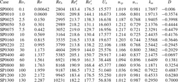
time units. The parameters and several statistics are listed in table 1.
Rotation number based on the global wall friction velocity (
 $Ro_{{\it\tau}}$
), rotation and Reynolds numbers based on the mean bulk velocity (
 $Ro$
and
 $Re_{b}$
), friction Reynolds number at the pressure and suction walls (
 $Re_{{\it\tau}}^{p}=u_{{\it\tau}p}^{\ast }h^{\ast }/{\it\nu}^{\ast }$
and
 $Re_{{\it\tau}}^{s}=u_{{\it\tau}s}^{\ast }h^{\ast }/{\it\nu}^{\ast }$
), normalized mean bulk velocity (
 $U_{b}$
), normalized local friction velocities at the pressure and suction walls (
 $u_{{\it\tau}p}=u_{{\it\tau}p}^{\ast }/u_{{\it\tau}}^{\ast }$
and
 $u_{{\it\tau}s}=u_{{\it\tau}s}^{\ast }/u_{{\it\tau}}^{\ast }$
), volume-averaged turbulent kinetic energy (
 $k_{m}$
) and the intercept
 $D$
of the Reynolds shear stress with the
 $y$
-axis defined by (3.2).

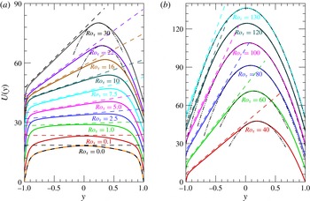
Mean velocity profiles of
 $U(y)$
versus
 $y$
: (a) for
 $0\leqslant Ro_{{\it\tau}}\leqslant 30$
(
 $0\leqslant Ro\leqslant 1.173$
); (b) for
 $40\leqslant Ro_{{\it\tau}}\leqslant 130$
(
 $1.337\leqslant Ro\leqslant 2.287$
). The dashed lines are the
 $2{\it\Omega}$
-slope lines and the dash-double-dotted lines are parabolas with
 $U(y)=-Re_{{\it\tau}}(y-M)^{2}/2+N$
, see (3.6) below. The lines are shifted upward for clarity.

3. Results
In figure 2, the mean velocity profiles for all of our cases are depicted. It is clearly seen that there is a region near the pressure side where the slope of the mean velocity is approximately twice the system rotation rate, that is,
 $\text{d}(U^{\ast })/\text{d}(y^{\ast })\approx 2{\it\Omega}^{\ast }$
, and this leads to
 $\text{d}U/\text{d}y=\text{d}(U^{\ast }/u_{{\it\tau}}^{\ast })/\text{d}(y^{\ast }/h^{\ast })\approx 2{\it\Omega}^{\ast }h^{\ast }/u_{{\it\tau}}^{\ast }=Ro_{{\it\tau}}$
. The location and extent of this region vary with the rotation number. The start location shifts to the pressure-side wall monotonically as the rotation number increases. However, this is not the case for the extent of the linear mean velocity region. At lower rotation number, the
 $2{\it\Omega}^{\ast }$
-slope extent increases with the rotation number, but it decreases for increasing rotation number at high rotation number (
 $Ro_{{\it\tau}}\gtrsim 40$
, or
 $Ro\gtrsim 1.337$
).
In wall-bounded turbulent flows without separation and rotation, a universal logarithmic behaviour has been reported for the normalized streamwise velocity fluctuations, in addition to the logarithmic behaviour of the mean streamwise velocity (Perry, Henbest & Chong Reference Perry, Henbest and Chong1986; Marusic et al.
Reference Marusic, Monty, Hultmark and Smits2013; Meneveau & Marusic Reference Meneveau and Marusic2013; Stevens, Wilczek & Meneveau Reference Stevens, Wilczek and Meneveau2014). However, in spanwise-rotating turbulent channel flow, a clear
 $2{\it\Omega}^{\ast }$
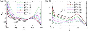
-slope region can be identified instead of the logarithmic behaviour. Whether there is any quantitative relationship between the r.m.s. value of the streamwise velocity fluctuations and the wall distance is unknown. In figure 3, we show the r.m.s. value of the streamwise velocity fluctuations
 $u_{rms}^{\prime }$
for
 $1.0\leqslant Ro_{{\it\tau}}\leqslant 130$
(
 $0.06\leqslant Ro\leqslant 2.287$
), where a linear behaviour can be clearly observed near the pressure (unstable) side when
 $Ro_{{\it\tau}}\gtrsim 2.5$
(
 $Ro\gtrsim 0.15$
). This linear region appears to coincide with the extent of the
 $2{\it\Omega}^{\ast }$
-slope region of the mean velocity profile shown in figure 2. The slope, which is approximately
 $-0.43$
, seems to be independent of the rotation number.
Root mean square value of the streamwise velocity fluctuations
 $u_{rms}^{\prime }$
: (a) for
 $1.0\leqslant Ro_{{\it\tau}}\leqslant 30$
(
 $0.06\leqslant Ro\leqslant 1.173$
); (b) for
 $30\leqslant Ro_{{\it\tau}}\leqslant 130$
(
 $1.173\leqslant Ro\leqslant 2.287$
).

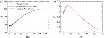
(a) Bulk mean velocity
 $U_{b}$
and (b) volume-averaged turbulent kinetic energy
 $k_{m}$
as a function of
 $Ro_{{\it\tau}}$
. The bulk velocity data from Grundestam et al. (Reference Grundestam, Wallin and Johansson2008a
) and Yang & Wu (Reference Yang and Wu2012) are also given for comparison.

In addition to the
 $2{\it\Omega}^{\ast }$
-slope of the mean velocity profile, the system rotation also results in changes of the mean bulk velocity and turbulent kinetic energy, and the normalized bulk mean velocity
 $U_{b}$
and volume-averaged turbulent kinetic energy
 $k_{m}$
are shown in figure 4. The bulk mean velocity data from Grundestam et al. (Reference Grundestam, Wallin and Johansson2008a
) and Yang & Wu (Reference Yang and Wu2012) are also shown in figure 4(a) for comparison. The results show that our data are in good agreement with those previously reported results, which confirms the accuracy of the present simulations. It is apparent from figure 4(a) that
 $U_{b}$
increases with
 $Ro_{{\it\tau}}$
, and this trend is more obvious for
 $Ro_{{\it\tau}}\gtrsim 16$
(
 $Ro\gtrsim 0.815$
). Differently from the bulk mean velocity, the change of the volume-averaged turbulent kinetic energy is non-monotonic, as shown in figure 4(b). It increases with the rotation number when
 $Ro_{{\it\tau}}\lesssim 16$
(
 $Ro\lesssim 0.815$
) and decreases at larger
 $Ro_{{\it\tau}}$
. These results demonstrate that the rotation of the system will not always damp the turbulence, but it will first augment the turbulence at lower rotation number. Furthermore, the rapid increase of
 $U_{b}$
and the decay of
 $k_{m}$
occur in almost the same rotation number region, which may imply that the energy input (due to the system rotation) mostly enters into the turbulent fluctuations at lower rotation number, and the energy flows back to the mean velocity for strong rotation due to the presence of inverse energy cascades (Grundestam et al.
Reference Grundestam, Wallin and Johansson2008a
; Yang & Wu Reference Yang and Wu2012). In fact, by analysing the balance of the Reynolds stress transport equations, Grundestam et al. (Reference Grundestam, Wallin and Johansson2008a
) reported a negative production term of turbulent kinetic energy in a layer adjacent to the location with the maximal mean streamwise velocity at the stable side at
 $Ro=1.50$
(which corresponds to
 $Ro_{{\it\tau}}=55.0$
), documenting that the energy is taken from the turbulence and fed back into the mean flow. Furthermore, by using the helical wave decomposition, Yang & Wu (Reference Yang and Wu2012) found that the region where the energy flux function
 ${\it\Pi}(K)$
is negative appears at small
 $K$
, and the extent and right boundary of the region extend rightwards as
 $Ro$
increases, illustrating that pure fluctuating energy is transferred from small scales to larger ones due to the nonlinear interaction among the fluctuating modes. (Here,
 ${\it\Pi}(K)$
represents the energy flux through wavenumber
 $K$
to all of the modes with wavenumber larger than
 $K$
by the nonlinear interaction of the fluctuating modes. See Yang & Wu (Reference Yang and Wu2012) for more details.)
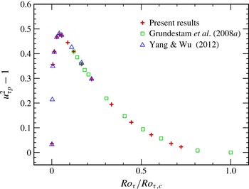
The change of
 $(u_{{\it\tau}p}^{2}-1)$
as a function of
 $(Ro_{{\it\tau}}/Ro_{{\it\tau},c})$
. The data from Grundestam et al. (Reference Grundestam, Wallin and Johansson2008a
) and Yang & Wu (Reference Yang and Wu2012) are also given for comparison.

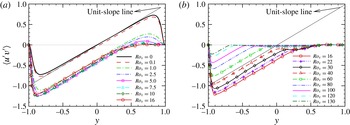
Reynolds shear stresses profiles: (a) for
 $0\leqslant Ro_{{\it\tau}}\leqslant 16$
(
 $0\leqslant Ro\leqslant 0.815$
); (b) for
 $16\leqslant Ro_{{\it\tau}}\leqslant 130$
(
 $0.815\leqslant Ro\leqslant 2.287$
). The solid line that starts at
 $(-1,-1)$
is the unit-slope straight line.

The system rotation also affects the local wall-shear velocities on both the pressure and suction sides. The change of
 $(u_{{\it\tau}p}^{2}-1)$
as a function of
 $(Ro_{{\it\tau}}/Ro_{{\it\tau},c})$
is shown in figure 5. Here,
 $Ro_{{\it\tau},c}\approx 180$
(
 $Ro_{c}\approx 3.0$
) is the critical rotation number at
 $Re_{{\it\tau}}=180$
, which corresponds to the laminar limit (Grundestam et al.
Reference Grundestam, Wallin and Johansson2008a
). As reported by Grundestam et al. (Reference Grundestam, Wallin and Johansson2008a
), the local friction velocity at the pressure side first increases with the rotation number for
 $Ro\lesssim 0.5$
and then decreases. In our study, the peak of
 $(u_{{\it\tau}p}^{2}-1)$
is located between
 $Ro_{{\it\tau}}=7.5$
(
 $Ro=0.442$
) and
 $Ro_{{\it\tau}}=10$
(
 $Ro=0.569$
), and the interpolated value is approximately
 $Ro_{{\it\tau}}=8.5$
. From figure 5, our data appear to be well matched to the data by Grundestam et al. (Reference Grundestam, Wallin and Johansson2008a
) and Yang & Wu (Reference Yang and Wu2012), which supports the choice of resolution and sampling duration for the present study, as described in § 2. It should be noted that this turning point
 $Ro_{{\it\tau}}\approx 8.5$
is smaller than the one for the turbulent kinetic energy (approximately half of it). However,
 $u_{{\it\tau}s}^{2}-1=-(u_{{\it\tau}p}^{2}-1)$
shows the opposite trend. (Interestingly, the change of
 $(u_{{\it\tau}p}^{2}-1)$
as a function of
 $(x\equiv Ro_{{\it\tau}}/Ro_{{\it\tau},c})$
can be approximated by a function
 $y=a\ast \sin ^{b}(x^{p}{\rm\pi})$
, with
 $a=0.48$
,
 $b=2$
and
 $p=0.225$
, very well. Furthermore, considering
 $Ro_{{\it\tau},c}=Re_{{\it\tau}}$
, then
 $Ro_{{\it\tau}}/Ro_{{\it\tau},c}=Ro_{{\it\tau}}/Re_{{\it\tau}}=2{\it\Omega}^{\ast }{\it\nu}^{\ast }/(u_{{\it\tau}}^{\ast })^{2}$
, which is twice the Coriolis parameter used by Nakabayashi & Kitoh (Reference Nakabayashi and Kitoh1996).)
The Reynolds shear stress is of great importance in spanwise-rotating channel flow since it enters the spatially and temporally averaged governing equation (2.4) explicitly. The behaviour of the Reynolds shear stress has been extensively studied, see, e.g., Kristoffersen & Andersson (Reference Kristoffersen and Andersson1993) and Grundestam et al. (Reference Grundestam, Wallin and Johansson2008a
). Here, we would like to first present some general observations about the Reynolds shear stresses
 $\langle u^{\prime }v^{\prime }\rangle$
based on our data over a wider range of rotation number, see figure 6. At very small rotation rate,
 $Ro_{{\it\tau}}=0.1$
, the action of the Coriolis force can be considered as a perturbation to the non-rotating case (Kristoffersen & Andersson Reference Kristoffersen and Andersson1993), and the profile of
 $\langle u^{\prime }v^{\prime }\rangle$
shifts down a little from that of the non-rotating case. As the system rotates faster with
 $Ro_{{\it\tau}}\geqslant 1.0$
(
 $Ro\geqslant 0.06$
), the profile shifts downwards considerably and strong asymmetry is observed. At
 $Ro_{{\it\tau}}\approx 5.0$
(
 $Ro\approx 0.301$
), the Reynolds shear stress reaches its extreme value at the pressure side, and the profiles from
 $Ro_{{\it\tau}}=5.0,~7.5$
and 10 (
 $Ro=0.301,~0.442$
and 0.569) almost collapse onto each other in the region
 $-1\leqslant y\lesssim 0$
. For
 $Ro_{{\it\tau}}\geqslant 10$
(
 $Ro\geqslant 0.569$
), the absolute peak value of
 $\langle u^{\prime }v^{\prime }\rangle$
decreases as
 $Ro_{{\it\tau}}$
increases.
As discussed above, there is a
 $2{\it\Omega}^{\ast }$
-slope region near the pressure-side wall where
 $\text{d}U/\text{d}y\approx Ro_{{\it\tau}}$
. According to (2.10), we have
 $$\begin{eqnarray}\displaystyle \langle u^{\prime }v^{\prime }\rangle =y+(1-u_{{\it\tau}p}^{2})+\frac{1}{Re_{{\it\tau}}}\frac{\text{d}U}{\text{d}y}\approx y+(1-u_{{\it\tau}p}^{2})+\frac{Ro_{{\it\tau}}}{Re_{{\it\tau}}}=y+D, & & \displaystyle\end{eqnarray}$$
where the intercept
 $D$
at
 $y=0$
is
 $$\begin{eqnarray}\displaystyle D=1-u_{{\it\tau}p}^{2}+Ro_{{\it\tau}}/Re_{{\it\tau}}. & & \displaystyle\end{eqnarray}$$
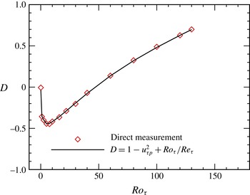
The intercept
 $D$
as a function of
 $Ro_{{\it\tau}}$
.

We display in figure 6(a,b) a linear line with unit slope, and it turns out that a distinct unit-slope region can be detected near the pressure side for
 $Ro_{{\it\tau}}\gtrsim 1.0$
(
 $Ro\gtrsim 0.06$
). At
 $Ro_{{\it\tau}}=0.1$
(
 $Ro=0.00642$
), the unit-slope region is not so obvious, and neither is the
 $2{\it\Omega}^{\ast }$
-slope of the mean velocity profile. The direct measurements of
 $D$
from figure 6 and the definition (3.2) are plotted versus
 $Ro_{{\it\tau}}$
in figure 7, and they match very well with each other, confirming the above conclusion that the Reynolds shear stress is linear with unit slope in the
 $2{\it\Omega}^{\ast }$
-slope region of the mean velocity, that is (3.1).
From figures 6 and 7, we can also see that the intercept
 $D$
at
 $y=0$
increases with
 $Ro_{{\it\tau}}$
when
 $Ro_{{\it\tau}}\gtrsim 8.5$
, and a limit value of 1.0 can be conjectured when
 $Ro_{{\it\tau}}$
reaches the critical laminar limit rotation number
 $Ro_{{\it\tau},c}$
. Therefore, we predict
 $Ro_{{\it\tau},c}=Re_{{\it\tau}}$
, since
 $1-u_{{\it\tau}p}^{2}=0$
when
 $Ro_{{\it\tau}}=Ro_{{\it\tau},c}$
. This is verified for
 $Re_{{\it\tau}}=180$
, where
 $Ro_{{\it\tau},c}\approx 180$
(Grundestam et al.
Reference Grundestam, Wallin and Johansson2008a
).
In fact, in the
 $2{\it\Omega}^{\ast }$
-slope region of the mean velocity, linear behaviour can also be identified for the production terms of
 $\langle u^{\prime }u^{\prime }\rangle$
and the turbulent kinetic energy. According to the governing equations for Reynolds stresses (Johnston et al.
Reference Johnston, Halleen and Lezius1972; Kristoffersen & Andersson Reference Kristoffersen and Andersson1993; Grundestam et al.
Reference Grundestam, Wallin and Johansson2008a
), the production term of
 $\langle u^{\prime }u^{\prime }\rangle$
is
 $$\begin{eqnarray}\displaystyle P_{11}=-2\langle u^{\prime }u_{j}^{\prime }\rangle \frac{\partial U}{\partial x_{j}}=-2\langle u^{\prime }v^{\prime }\rangle \frac{\text{d}U}{\text{d}y}=-2Ro_{{\it\tau}}(y+D). & & \displaystyle\end{eqnarray}$$
Then, the production term of the turbulent kinetic energy
 $k$
is
 $$\begin{eqnarray}\displaystyle P_{k}=P_{11}/2=-Ro_{{\it\tau}}(y+D). & & \displaystyle\end{eqnarray}$$
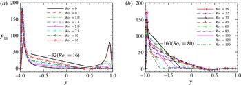
Figure 8 shows the production term of
 $\langle u^{\prime }u^{\prime }\rangle$
at different rotation numbers. Linear sections can be clearly identified from the figure. Two rotation numbers,
 $Ro_{{\it\tau}}=16$
(
 $Ro=0.815$
) and
 $Ro_{{\it\tau}}=80$
(
 $Ro=1.763$
), are used to identify the slopes of the linear sections, and clearly the slope of
 $P_{11}$
equals
 $-2Ro_{{\it\tau}}$
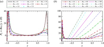
, as predicted. In order to further verify this linear behaviour of the production term, we depict in figure 9 the compensated form of the production term of
 $k$
, which is
 $P_{k}+Ro_{{\it\tau}}(y+D)$
, at different rotation numbers. Apparent plateaus can be observed around the
 $P_{k}+Ro_{{\it\tau}}(y+D)=0$
line for
 $Ro_{{\it\tau}}\gtrsim 1.0$
(
 $Ro\gtrsim 0.06$
), which confirms the linear profiles of
 $P_{k}$
and
 $P_{11}$
, as predicted by (3.4) and (3.3) respectively.
Production term of
 $\langle u^{\prime }u^{\prime }\rangle$
: (a) for
 $0\leqslant Ro_{{\it\tau}}\leqslant 16$
(
 $0\leqslant Ro\leqslant 0.815$
); (b) for
 $16\leqslant Ro_{{\it\tau}}\leqslant 130$
(
 $0.815\leqslant Ro\leqslant 2.287$
).

Compensated form of the production term of
 $k$
(
 $P_{k}+Ro_{{\it\tau}}$
(
 $y+D$
)): (a) for
 $0\leqslant Ro_{{\it\tau}}\leqslant 16$
(
 $0\leqslant Ro\leqslant 0.815$
); (b) for
 $16\leqslant Ro_{{\it\tau}}\leqslant 130$
(
 $0.815\leqslant Ro\leqslant 2.287$
).

It was reported by Grundestam et al. (Reference Grundestam, Wallin and Johansson2008a
) that there is a ‘second plateau’ of the Reynolds shear stress, and this is confirmed by our simulations, as depicted in figure 6 for
 $Ro_{{\it\tau}}\geqslant 22$
(
 $Ro\geqslant 0.995$
). At this plateau, the Reynolds shear stress is constant, which results in
 $$\begin{eqnarray}\displaystyle \frac{1}{Re_{{\it\tau}}}\frac{\text{d}U}{\text{d}y}=-y-(1-u_{{\it\tau}p}^{2})+\langle u^{\prime }v^{\prime }\rangle =-y+M, & & \displaystyle\end{eqnarray}$$
where
 $M=\langle u^{\prime }v^{\prime }\rangle -1+u_{{\it\tau}p}^{2}$
is also a constant at given
 $Ro$
. This leads to
 $$\begin{eqnarray}\displaystyle U(y)=-\frac{Re_{{\it\tau}}}{2}(y-M)^{2}+N, & & \displaystyle\end{eqnarray}$$
demonstrating the parabolic feature of the mean velocity. Here,
 $N$
is the maximum mean velocity across the channel and
 $M$
is the symmetric axis of the parabola which indicates the location of the maximum mean velocity. We have plotted several parabolas in figure 2, and they match with the mean velocity profiles very well for
 $Ro_{{\it\tau}}\geqslant 22$
(
 $Ro\geqslant 0.995$
). Specifically, all parabolas have the same shape, that is, they open in the negative direction and have the same radius of curvature at the vertex (
 $1/Re_{{\it\tau}}$
). The matched region enlarges as the rotation number increases, and so does the plateau region. Furthermore, as
 $Ro_{{\it\tau}}$
increases, the value of
 $\langle uv\rangle$
at the ‘second plateau’ approaches zero, and so does the value of
 $M$
. At
 $Ro_{{\it\tau}}=130$
(
 $Ro=2.287$
), the parabola matches with the mean velocity profile very well for
 $y/h\gtrsim -0.65$
and its axis of symmetry is located at
 $y=M\approx 0.016$
. At the laminar limit
 $Ro_{{\it\tau},c}\approx 180$
, the mean velocity profile becomes fully parabolic with an axis of symmetry located at the channel centre.
It was shown in figure 4(b) that the volume-averaged turbulent kinetic energy first increases with the rotation number for
 $Ro_{{\it\tau}}\leqslant 16$
(
 $Ro\leqslant 0.815$
) and then decreases when
 $Ro_{{\it\tau}}\geqslant 16$
(
 $Ro\geqslant 0.815$
). However, the distribution of turbulent kinetic energy across the channel width at each rotation number is not obvious, although its three shares
 $\langle u^{\prime }u^{\prime }\rangle$
,
 $\langle v^{\prime }v^{\prime }\rangle$
and
 $\langle w^{\prime }w^{\prime }\rangle$
were shown before by Kristoffersen & Andersson (Reference Kristoffersen and Andersson1993) and Grundestam et al. (Reference Grundestam, Wallin and Johansson2008a
). This is due to the fact that the distributions of these shares never follow the same trend as the rotation number increases. Although they all decrease at the suction side as the rotation becomes stronger, their behaviours near the pressure side are not the same. For
 $\langle u^{\prime }u^{\prime }\rangle$
, its peak value first increases with the rotation number when
 $Ro\leqslant 1.0$
(
 $Ro\leqslant 0.06$
), and then decreases with it. The peak is larger than that of the non-rotating case when
 $0<Ro_{{\it\tau}}<5.0$
(
 $0<Ro<0.301$
). For
 $\langle v^{\prime }v^{\prime }\rangle$
and
 $\langle w^{\prime }w^{\prime }\rangle$
, however, their peak values first increase with rotation number when
 $Ro\lesssim 40$
(
 $Ro\lesssim 1.337$
), and then decreases with it. Furthermore, the peak of
 $\langle w^{\prime }w^{\prime }\rangle$
is located closer to the pressure-side wall than that of
 $\langle v^{\prime }v^{\prime }\rangle$
, and a second peak emerges for
 $\langle w^{\prime }w^{\prime }\rangle$
when
 $22\lesssim Ro_{{\it\tau}}\leqslant 130$
(
 $0.995\lesssim Ro\leqslant 2.287$
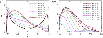
) (not shown here). Figure 10 shows the mean profiles of the turbulent kinetic energy
 $k$
at different rotation numbers. It is clearly seen that the turbulence is suppressed near the suction side at all rotation numbers considered, while the change near the pressure side is not monotonic. At small rotation number
 $Ro\leqslant 1.0$
(
 $Ro\leqslant 0.06$
), it is augmented near the pressure side due to the increases of its three shares (in this rotation number region, the turbulent kinetic energy increases). As the system rotates faster, the local peak value decreases while its location moves closer to the wall. At the same time, the turbulent kinetic energy increases near the
 $2{\it\Omega}^{\ast }$
-slope region of the mean velocity and a second peak emerges around
 $y^{\ast }=-0.6h$
when
 $Ro_{{\it\tau}}\geqslant 7.5$
(
 $Ro\geqslant 0.442$
), and this is due to the higher values of
 $\langle w^{\prime }w^{\prime }\rangle$
and
 $\langle v^{\prime }v^{\prime }\rangle$
in this region. At
 $Ro_{{\it\tau}}=10$
, the second peak value is very close to (although smaller than) the first one, but it is much larger than the first one at
 $Ro_{{\it\tau}}=16$
(
 $Ro=0.815$
). At approximately
 $Ro_{{\it\tau}}=30$
(
 $Ro=1.173$
), the first peak disappears, leaving the second one as the only peak. After that, the turbulent kinetic energy decays across the channel as the rotation number increases.
Mean profiles of the turbulent kinetic energy: (a) for
 $0\leqslant Ro_{{\it\tau}}\leqslant 16$
(
 $0\leqslant Ro\leqslant 0.815$
); (b) for
 $16\leqslant Ro_{{\it\tau}}\leqslant 130$
(
 $0.815\leqslant Ro\leqslant 2.287$
).

4. Conclusion and discussion
In this paper, a series of DNS on pressure-driven channel flow with spanwise rotation is performed. The global friction Reynolds number is fixed at
 $Re_{{\it\tau}}=180$
, while the global-friction-velocity-based rotation number
 $Ro_{{\it\tau}}$
varies from 0 to 130. Our work focuses on the new quantitative behaviour of the mean velocity profile, the r.m.s. value of the streamwise velocity fluctuations, the Reynolds shear stress profile, the production terms of
 $\langle u^{\prime }u^{\prime }\rangle$
and the turbulent kinetic energy, and the changes of the turbulent kinetic energy due to the system rotation.
It has been reported before, and verified in the present simulations, that there is a
 $2{\it\Omega}^{\ast }$
-slope region near the pressure side for the mean velocity profile. In this linear region, the r.m.s. value of the streamwise velocity fluctuations, the Reynolds shear stress and the production terms of
 $\langle u^{\prime }u^{\prime }\rangle$
and the turbulent kinetic energy are found to exhibit linear behaviour too. The slopes of the r.m.s. value of the streamwise velocity fluctuations and the Reynolds shear stress are
 $-0.43$
and
 $1$
respectively, while those of the production terms of
 $\langle u^{\prime }u^{\prime }\rangle$
and the turbulent kinetic energy are
 $-2Ro_{{\it\tau}}$
and
 $-Ro_{{\it\tau}}$
. From the limiting behaviour of the linear profile of the Reynolds shear stress, we infer that the critical laminar limit rotation number
 $Ro_{{\it\tau},c}$
should be equal to the friction Reynolds number
 $Re_{{\it\tau}}$
. Furthermore, a ‘second plateau’ of the Reynolds shear stress is confirmed in our simulation for
 $Ro_{{\it\tau}}\geqslant 22$
(
 $Ro\geqslant 0.995$
), and this leads to a parabolic profile of the mean velocity in this region. The parabolas at different rotation numbers have the same shape of
 $1/Re_{{\it\tau}}$
, the radius of curvature at the vertex. As the system rotates faster, this parabolic region enlarges and finally covers the whole channel when the rotation number reaches its laminar limit
 $Ro_{{\it\tau},c}$
. These quantitative results provide new information for researchers who intend to develop or assess RANS and/or LES models for problems subjected to system rotation.
Although the rotation in the spanwise direction stabilizes the flow at the suction side and destabilizes it at the pressure side, the overall effect on the turbulence is non-monotonic based on the studies of the volume-averaged turbulent kinetic energy and the turbulent kinetic energy profiles along the wall-normal direction. At smaller rotation number, the turbulent augmentation on the pressure side is much stronger than the suppression on the suction side, resulting in an increase of the volume-averaged turbulent kinetic energy. As the rotation becomes stronger, the first peak value of the turbulent kinetic energy profile decreases and a second peak emerges in the
 $2{\it\Omega}^{\ast }$
-slope region of the mean velocity. At approximately
 $Ro_{{\it\tau}}\approx 16$
(
 $Ro\approx 0.815$
), the volume-averaged turbulent kinetic energy reaches its maximum. At higher rotation number, the second peak becomes the only peak of the kinetic energy profile, and it decays all over the channel as the system rotates faster.
The linear behaviour of the Reynolds shear stress and the production terms of
 $\langle u^{\prime }u^{\prime }\rangle$
and the turbulent kinetic energy can be easily verified through a simple derivation from the mean momentum equation and the definition of the production term. However, we cannot provide any theoretical derivation for the linear behaviour of the r.m.s. value of the streamwise velocity fluctuations. In the future, we intend to study this linear behaviour through both numerical and theoretical approaches, as well as the behaviour of high-order moments of the streamwise velocity fluctuations.
Acknowledgements
The numerical simulations were finished at the National Supercomputer Centers in Tianjin (Tianhe-1A), China. We acknowledge the financial support provided by the National Natural Science Foundation of China (grant nos 91130001, 11221061 and 11302006). The authors would like to thank Professor J. Wu for many useful discussions and suggestions.