1 Introduction
Consider the family of quadratic polynomials
 $$ \begin{align*}f_{c}(z)=z^{2}+c,\quad c\in{\mathbb{C}}. \end{align*} $$
We say that a parameter
 $c_{0}\in {\mathbb {C}}$
is a critical point of a period n multiplier if the map
 $f_{c_{0}}$
has a periodic orbit of period n, whose multiplier, viewed as a locally analytic function of c, has a vanishing derivative at
 $c=c_{0}$
. The study of critical points of the multipliers is motivated by the problem of understanding the geometry of hyperbolic components of the Mandelbrot set.
As it was observed by Sullivan and Douady and Hubbard [Reference Douady and Hubbard4], the argument of quasiconformal surgery implies that the multipliers of periodic orbits, viewed as analytic functions of the parameter c, are Riemann mappings of the corresponding hyperbolic components of the Mandelbrot set. Existence of analytic extensions of the inverse branches of these Riemann mappings to larger domains can be helpful in estimating the geometry of the hyperbolic components as well as the sizes of some limbs of the Mandelbrot set [Reference Levin8–Reference Levin10] (see also [Reference Dezotti3]). Critical values of the multipliers are the only obstructions to the existence of these analytic extensions.
It is of special interest to obtain uniform bounds on the shapes of hyperbolic components within renormalization cascades. In particular, this motivates the study of the asymptotic behavior of the critical points of period n multipliers as
 $n\to \infty $
. In [Reference Firsova and Gorbovickis5], the current authors approached this question from the statistical point of view and proved that the critical points of the period n multipliers equidistribute on the boundary of the Mandelbrot set as
 $n\to \infty $
.
More specifically, for each
 $n\in {\mathbb {N}}$
, let
 $X_{n}$
be the set of all parameters
 $c\in {\mathbb {C}}$
that are critical points of a period n multiplier (counted with multiplicities). Let
 ${\mathbb M}\subset {\mathbb {C}}$
denote the Mandelbrot set and let
 ${\mu _{\mathrm {bif}}}$
be its equilibrium measure (or the bifurcation measure of the quadratic family
 $\{f_{c}\}$
). Let
 $\delta _{x}$
denote the
 $\delta $
-measure at
 $x\in {\mathbb {C}}$
. Then the following theorem is obtained.
Theorem 1.1. [Reference Firsova and Gorbovickis5]
The sequence of probability measures
 $$ \begin{align*}\frac{1}{\# X_{n}}\sum_{x\in X_{n}}\delta_{x} \end{align*} $$
converges to the equilibrium measure
 ${\mu _{\mathrm {bif}}}$
in the weak sense of measures on
 ${\mathbb {C}}$
as
 $n\to \infty $
.
At the same time, it was shown in [Reference Belova and Gorbovickis1] that
 $0$
is a critical point of infinitely many multipliers of different periodic orbits, and hence, since
 $0\not \in \partial {\mathbb M}=\mathrm {supp}({\mu _{\mathrm {bif}}})$
, this implies that as the period n grows to infinity, the critical points of period n multipliers accumulate on some set
 $\mathcal X\subset {\mathbb {C}}$
that is strictly greater than the support of the bifurcation measure
 ${\mu _{\mathrm {bif}}}$
.
The purpose of the current paper is to study this accumulation set
 $\mathcal X$
which can formally be defined as
 $$ \begin{align*} \mathcal X:= \bigcap_{k=1}^{\infty} \bigg(\,\overline{\bigcup_{n=k}^{\infty} X_{n}} \,\bigg). \end{align*} $$
We note that the study of the accumulation set
 $\mathcal X$
complements the statistical approach of Theorem 1.1 in the attempt to understand asymptotic behavior of the critical points of the multipliers.
The first result of this paper is the following.
Theorem A. The accumulation set
 $\mathcal X$
is bounded, connected, and contains the Mandelbrot set
 ${\mathbb M}$
. Furthermore, the set
 $\mathcal X\setminus {\mathbb M}$
is nonempty and has a nonempty interior.
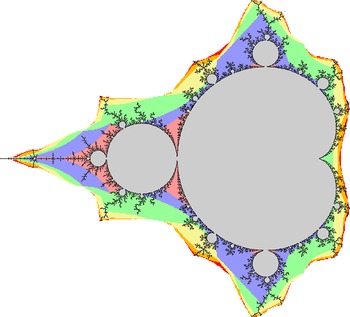
Figure 1 provides a numerical approximation of the accumulation set
 $\mathcal X$
. We also note that the last part of Theorem A complements the following result, previously obtained by the authors in [Reference Firsova and Gorbovickis5].
The set
 $\mathcal X$
is numerically approximated by the union of the Mandelbrot set and the colored regions. The algorithm for the construction of this picture, as well as the meaning of the colors, are explained in Appendix A.

Theorem 1.2. [Reference Firsova and Gorbovickis5]
If
 $c\in {\mathbb {C}}\setminus {\mathbb M}$
is a critical point of some multiplier, then
 $c\in \mathcal X$
. Equivalently, the following identity holds:
 $$ \begin{align*} \overline{\bigcup_{n=1}^{\infty} (X_{n}\setminus{\mathbb M})} =\mathcal X\setminus{\mathbb M}. \end{align*} $$
We need a few more definitions to state our next result. For a periodic orbit
 $\mathcal O$
of some map
 $f_{c}$
, let
 $\lvert {\mathcal O}\rvert $
stand for its period (that is, the number of distinct points in it).
We recall that a periodic orbit is called primitive parabolic if its multiplier is equal to
 $1$
. As discussed in [Reference Firsova and Gorbovickis5], for every
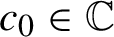 $c_{0}\in {\mathbb {C}}$
and every periodic orbit
 $\mathcal O$
of
 $f_{c_{0}}$
that is not primitive parabolic, the multiplier of this periodic orbit can be viewed as a locally analytic function of the parameter c in the neighborhood of
 $c_{0}$
. We denote this function by
 $\rho _{\mathcal O}$
. If in addition to that,
 $\rho _{\mathcal O}(c_{0})\neq 0$
, one can consider a locally analytic function
 $\nu _{\mathcal O}$
, defined in a neighborhood of
 $c_{0}$
by the formula
 $$ \begin{align} \nu_{\mathcal O}(c):= \frac{\rho^{\prime}_{\mathcal O}(c)}{\lvert{\mathcal O}\rvert\,\rho_{\mathcal O}(c)}. \end{align} $$
For each
 $c\in {\mathbb {C}}$
, let
 $\Omega _{c}$
denote the set of all repelling periodic orbits of the map
 $f_{c}$
. In particular, the locally analytic maps
 $\nu _{\mathcal O}$
are defined for all
 $\mathcal O\in \Omega _{c}$
in corresponding neighborhoods of the parameter c.
For each
 $c\in {\mathbb {C}}$
, we consider the set
 $\mathcal Y_{c}\subset {\mathbb {C}}$
, defined by
 $$ \begin{align*}\mathcal Y_{c}:= \overline{\{\nu_{\mathcal O}(c) \mid \mathcal O\in\Omega_{c}\}}. \end{align*} $$
Our second result is the following.
Theorem B. The following two properties hold.
-
(i) For every parameter
 $c\in {\mathbb {C}}\setminus \{-2\}$
, the set
$\mathcal Y_{c}$
is convex; for
$c=-2$
, the set
$\mathcal Y_{-2}$
is the union of a convex set and the point
$-\tfrac 16$
.
-
(ii) For every parameter
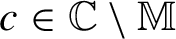
$c\in {\mathbb {C}}\setminus {\mathbb M}$
, the set
$\mathcal Y_{c}$
is bounded. A parameter
$c\in {\mathbb {C}}\setminus {\mathbb M}$
belongs to
$\mathcal X$
if and only if
$0\in \mathcal Y_{c}$
.




We note that the relation between the sets
 $\mathcal Y_{c}$
and
 $\mathcal X$
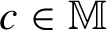
, described in part (ii) of Theorem B, resembles the relation between the filled Julia and the Mandelbrot sets, namely that
 $c\in {\mathbb M}$
if and only if
 $0$
belongs to the filled Julia set
 $K_{c}$
of
 $f_{c}$
.
As an application of our results and the results of [Reference He and Nie6], we deduce that the Hausdorff dimension function cannot have critical points outside of the accumulation set
 $\mathcal X$
. More specifically, let
 $\delta \colon {\mathbb {C}}\to {\mathbb {R}}$
be the function that assigns to each parameter
 $c\in {\mathbb {C}}$
the Hausdorff dimension of the Julia set of
 $f_{c}$
. It is known that the function
 $\delta $
is real-analytic in each hyperbolic component [Reference Bowen2] (including the complement of the Mandelbrot set). In [Reference He and Nie6, Theorem 1.3], He and Nie give a necessary condition for a hyperbolic parameter
 $c\in {\mathbb {C}}$
to be a critical point of the Hausdorff dimension function
 $\delta $
. Their result is stated for rational maps of degree d, rather than just quadratic polynomials, and the proof is based on ideas from thermodynamical formalism. In the special case of the quadratic family, we can restate their theorem in a concise form as follows.
Theorem 1.3. [Reference He and Nie6]
If
 $c\in {\mathbb {C}}$
is such that
 $f_{c}$
is a hyperbolic map and
 $c$
is a critical point for the map
 $\delta$
, then
 $0\in \mathcal Y_{c}$
.
Combining Theorem 1.3 with the main results of this paper, we obtain the following corollary.
Corollary 1.4. The Hausdorff dimension function
 $\delta $
has no critical points in
 ${\mathbb {C}}\setminus \mathcal X$
.
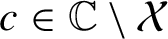
Proof. According to Theorem A, any parameter
 $c\in {\mathbb {C}}\setminus \mathcal X$
lies outside of the Mandelbrot set
 ${\mathbb M}$
, and hence the function
 $\delta $
is real-analytic at c. Furthermore, part (ii) of Theorem B implies that
 $0\not \in \mathcal Y_{c}$
, and hence, it follows from Theorem 1.3 that
 $c$
is not a critical point of the map
 $\delta$
.
1.1 Open questions
Finally, we list some further questions that can be addressed in the study of the geometry of the accumulation set
 $\mathcal X$
and the sets
 $\mathcal Y_{c}$
.
-
(1) Is the set
$\mathcal X$
path connected (see Remark 4.9)? Is it simply connected? -
(2) Does the boundary of the set
$\mathcal X$
possess any kind of self-similarity? Is the Hausdorff dimension of
$\partial \mathcal X$
equal to
$1$
or is it strictly greater than
$1$
? -
(3) For which
$c\in {\mathbb {C}}$
are the sets
$\mathcal Y_{c}$
polygonal? How are the points of the finite sets
$Y_{c,n}=\{\nu _{\mathcal O}(c)\mid \mathcal O\in \Omega _{c}, \lvert {\mathcal O}\rvert = n\}$
distributed inside
$\mathcal Y_{c}$
as
$n\to \infty $
? -
(4) What can we say about the geometry of the sets
$\mathcal Y_{c}$
when
$c\in \partial {\mathbb M}$
? Are these sets always unbounded?


2 On averaging several periodic orbits
In this section, we state and prove the so called averaging lemma which is the key component of the proofs of Theorems A and B.
Lemma 2.1. (Averaging lemma)
For any real
 $\alpha \in [0,1]$
, a complex parameter
 $c_{0}\in {\mathbb {C}}$
and any two distinct repelling periodic orbits
 $\mathcal O_{1}$
and
 $\mathcal O_{2}$
of
 $f_{c_{0}}$
, such that if
 $c_{0}=-2$
, then neither of the orbits
 $\mathcal O_{1}, \mathcal O_{2}$
is the fixed point
 $z=2$
, the following holds: there exist a neighborhood U of
 $c_{0}$
and a sequence of distinct repelling periodic orbits
 $\{\mathcal O_{j}\}_{j=3}^{\infty }$
of
 $f_{c_{0}}$
, such that the maps
 $\nu _{\mathcal O_{j}}$
are defined and analytic in U, for all
 $j\in {\mathbb {N}}$
, and the sequence of maps
 $\{\nu _{\mathcal O_{j}}\}_{j=3}^{\infty }$
converges to
 $\alpha \nu _{\mathcal O_{1}}+(1-\alpha )\nu _{\mathcal O_{2}}$
uniformly in U.
We need a few preliminary propositions before we can pass to the proof of Lemma 2.1.
For any
 $c_{0}\in {\mathbb {C}}$
and a periodic orbit
 $\mathcal O$
of
 $f_{c_{0}}$
that is non-critical and not primitively parabolic, let
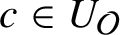
 $U_{\mathcal O}\subset {\mathbb {C}}$
be a simply connected neighborhood of
 $c_{0}$
, such that
 $\rho _{\mathcal O}(c)\neq 0$
for any
 $c\in U_{\mathcal O}$
and let
 $g_{\mathcal O}\colon U_{\mathcal O}\to {\mathbb {C}}$
be the analytic map defined by the relation
 $$ \begin{align} g_{\mathcal O}(c):= (\rho_{\mathcal O}(c))^{1/\lvert {\mathcal O}\rvert}, \end{align} $$
where the branch of the root is chosen so that
 $$ \begin{align*}\arg(g_{\mathcal O}(c_{0}))\in (-\pi/\lvert {\mathcal O}\rvert, \pi/\lvert{\mathcal O}\rvert]. \end{align*} $$
(A particular choice of the branch of the root is not important, but we prefer to make a definite choice.)
For further reference, let us make the following basic observation.
Proposition 2.2. For any
 $c_{0}\in {\mathbb {C}}$
, a non-critical periodic orbit
 $\mathcal O$
of
 $f_{c_{0}}$
and a neighborhood
 $U_{\mathcal O}\subset {\mathbb {C}}$
, satisfying the above conditions, we have
 $$ \begin{align*}\frac{d}{dc}[\log (g_{\mathcal O}(c))] = \nu_{\mathcal O}(c), \end{align*} $$
for all
 $c\in U_{\mathcal O}$
.
Proof. This follows from a basic computation.
Proposition 2.3. Assume
 $z_{0}\in {\mathbb {C}}$
is a periodic point that belongs to a repelling periodic orbit
 $\mathcal O$
of period n for a map
 $f_{c_{0}}$
, where
 $c_{0}\in {\mathbb {C}}$
is an arbitrary fixed parameter. Let
 $V\subset {\mathbb {C}}$
be a simply connected neighborhood of
 $z_{0}$
, such that
 $f_{c_{0}}^{\circ n}$
is univalent on V and the inclusion
 $V\Subset f_{c_{0}}^{\circ n}(V)$
holds. Then there exists a neighborhood
 $U\subset {\mathbb {C}}$
of
 $c_{0}$
, such that for all
 $c\in U$
, an appropriate branch
 $\phi _{c}$
of the inverse
 $f_{c}^{\circ (- n)}$
is defined on V, the inclusion
 $\phi _{c}(V)\Subset V$
holds, and for any
 $z\in V$
, the analytic functions
 $$ \begin{align*}h_{k,z}(c):= [(f_{c}^{\circ (nk)})^{\prime}(\phi_{c}^{\circ k}(z))]^{1/(nk)} \end{align*} $$
converge to
 $g_{\mathcal O}$
uniformly in
 $z\in V$
and
 $c\in U$
, for appropriate branches of the roots as
 $k\to \infty $
.
Proof. Since the inverse branch of
 $f_{c_{0}}^{\circ (- n)}$
, taking V compactly inside itself, is defined on a domain that compactly contains V, it follows that the same holds for
 $f_{c}^{\circ (- n)}$
, where c is any parameter from a sufficiently small neighborhood U of
 $c_{0}$
. For each
 $c\in U$
, let
 $\phi _{c}$
be such an inverse branch of
 $f_{c}^{\circ (- n)}$
.
According to Denjoy–Wolff theorem applied to the map
 $\phi _{c}$
, we conclude that for any
 $c\in U$
, the map
 $f_{c}^{\circ n}$
has a unique repelling fixed point
 $z_{c}$
that depends analytically on c and coincides with
 $z_{0}$
, when
 $c=c_{0}$
. This implies that the map
 $g_{\mathcal O}$
is defined for all
 $c\in U$
.
For any
 $c\in U$
and
 $z\in V$
, consider the sequence of points
 $z_{j} = \phi _{c}^{\circ j}(z)$
. Then the chain rule yields
 $$ \begin{align*}h_{k,z}(c) = \bigg(\prod_{j=1}^{k}(f_{c}^{\circ n})^{\prime}(z_{j})\bigg)^{1/(nk)}. \end{align*} $$
At the same time, we observe that according to the Koebe distortion theorem, after possibly shrinking the neighborhood U, there exists a constant
 $K>0$
, such that
 $$ \begin{align*}\frac{\lvert (f_{c}^{\circ n})^{\prime}(z_{c})\rvert}{K}<\lvert (f_{c}^{\circ n})^{\prime}(w)\rvert < K \lvert(f_{c}^{\circ n})^{\prime}(z_{c})\rvert\quad \text{for } c\in U, w\in \phi_{c}(V). \end{align*} $$
Finally, Denjoy–Wolff theorem implies that for any
 $c\in U$
and
 $z\in V$
, the sequence of points
 $z_{j}$
converges to
 $z_{c}$
uniformly in
 $z\in V$
as
 $k\to \infty $
. Hence, the geometric averages of
 $(f_{c}^{\circ n})^{\prime }(z_{1}),\ldots , (f_{c}^{\circ n})^{\prime }(z_{k})$
converge uniformly in
 $z\in V$
,
 $c\in U$
to
 $(f_{c}^{\circ n})^{\prime }(z_{c})$
. The latter implies
 $$ \begin{align*}\lim_{k\to\infty}h_{k,z}(c) = ((f_{c}^{\circ n})^{\prime}(z_{c}))^{1/n} = g_{\mathcal O}(c), \end{align*} $$
assuming that appropriate branches of the roots are chosen in the definition of
 $h_{k,z}(c)$
.
Proposition 2.4. Let
 $c,z_{0}\in {\mathbb {C}}$
be such that
 $z_{0}$
is a repelling periodic point of
 $f_{c}$
. Assume that
 $(c, z_{0})\neq (-2,2)$
. Then there exists a sequence
 $z_{-1}, z_{-2},z_{-3},\ldots \in {\mathbb {C}}$
, such that the following hold simultaneously:
-
(i) the sequence
$z_{-1}, z_{-2},z_{-3},\ldots $
is dense in the Julia set
$J_{c}$
; -
(ii)
$f(z_{-j})=z_{1-j}$
, for any
$j\in {\mathbb {N}}$
; -
(iii)
$z_{-j}\neq 0$
, for any
$j\in {\mathbb {N}}$
.


Proof. Existence of a sequence that satisfies properties (i) and (ii) follows immediately from the fact that the set of preimages of any point in the Julia set
 $J_{c}$
is dense in
 $J_{c}$
. Indeed, from any point
 $z_{-k}$
, one can land in any arbitrarily small region of
 $J_{c}$
by taking an appropriate sequence of preimages of
 $z_{-k}$
. We can continue this process, making sure that any arbitrarily small region of
 $J_{c}$
is eventually visited by our sequence. Furthermore, property (ii) implies that if
 $z_{-k}$
does not belong to the periodic orbit of
 $z_{0}$
, then for every
 $j\ge k$
, the element
 $z_{-j}$
is different from any other element of the entire sequence
 $z_{0},z_{-1},z_{-2},\ldots $
, no matter how the sequence of preimages of
 $z_{-k}$
was chosen.
Property (iii) is equivalent to the property that
 $z_{-j}\neq c$
for any
 $j\in {\mathbb {N}}\cup \{0\}$
, since c is the unique point that has only one preimage under the map
 $f_{c}$
, and that preimage is
 $0$
.
Let
 $\mathcal O$
be the periodic orbit of
 $f_{c}$
that contains
 $z_{0}$
. First of all, we note that
 $c\not \in \mathcal O$
. Otherwise, if
 $c\in \mathcal O$
, then
 $0\in \mathcal O$
, since
 $0$
is the unique preimage of c, and the orbit
 $\mathcal O$
is super-attracting, which contradicts the assumption of the proposition.
Assume that the sequence, constructed in the first paragraph of the proof, violates property (iii). Let
 $j\in {\mathbb {N}}$
be such that
 $z_{-j}=c$
. This number j is unique, since
 $c\not \in \mathcal O$
, so all further preimages of c must differ from c. If
 $z_{1-j}\not \in \mathcal O$
, then we can modify
 $z_{-j}$
by taking it to be equal to another preimage of
 $z_{1-j}$
. After that, we can construct the remaining ‘tail’ of the sequence by the same process, as described in the first paragraph. Since
 $z_{1-j}\not \in \mathcal O$
, no further element of the sequence will ever return to
 $z_{1-j}$
, and hence, the sequence is guaranteed to avoid the critical value c.
It follows from the construction described in the previous paragraph that the sequence
 $z_{-1},z_{-2},\ldots $
satisfying properties (i)–(iii) can be constructed, if at least one point of the periodic orbit
 $\mathcal O$
has a preimage under
 $f_{c}$
that does not belong to
 $\mathcal O$
and is not simultaneously equal to c. This condition is always satisfied, unless
 $z_{0}$
is a fixed point whose two preimages are
 $z_{0}$
and c. The latter happens only when
 $c=-2$
and
 $z_{0}=2$
.
Proof of Lemma 2.1
Let
 $n_{1}$
and
 $n_{2}$
be the periods of the periodic orbits
 $\mathcal O_{1}$
and
 $\mathcal O_{2}$
respectively. Let
 $z_{1}$
and
 $z_{2}$
be some periodic points from each of the orbits
 $\mathcal O_{1}$
and
 $\mathcal O_{2}$
. Since the orbits
 $\mathcal O_{1}$
and
 $\mathcal O_{2}$
are repelling, there exist a simply connected neighborhood U of
 $c_{0}$
and two neighborhoods
 $U_{1}$
and
 $U_{2}$
of
 $z_{1}$
and
 $z_{2}$
respectively, such that for all
 $c\in U$
, the maps
 $f_{c}^{\circ n_{1}}$
and
 $f_{c}^{\circ n_{2}}$
are univalent on
 $U_{1}$
and
 $U_{2}$
respectively, and
 $f_{c}^{\circ n_{1}}(U_{1})\setminus U_{1}$
and
 $f_{c}^{\circ n_{2}}(U_{2})\setminus U_{2}$
are two annuli.
According to Proposition 2.4, there exist
 $k_{1},k_{2}\in {\mathbb {N}}$
,
 $w_{1}\in U_{2}$
and
 $w_{2}\in U_{1}$
, such that
 $$ \begin{align*} f_{c_{0}}^{\circ k_{1}}(w_{1})&=z_{1}, \quad f_{c_{0}}^{\circ k_{2}}(w_{2})=z_{2},\\ (f_{c_{0}}^{\circ k_{1}})^{\prime}(w_{1})&\neq 0,\quad\text{and}\quad (f_{c_{0}}^{\circ k_{2}})^{\prime}(w_{2})\neq 0. \end{align*} $$
Possibly, after shrinking the neighborhood U of
 $c_{0}$
, there exist a constant
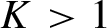 $K>1$
and the neighborhoods
 $V_{1}\Subset U_{2}$
and
 $V_{2}\Subset U_{1}$
of
 $w_{1}$
and
 $w_{2}$
respectively, such that for any
 $c\in U$
and
 $j\in \{1,2\}$
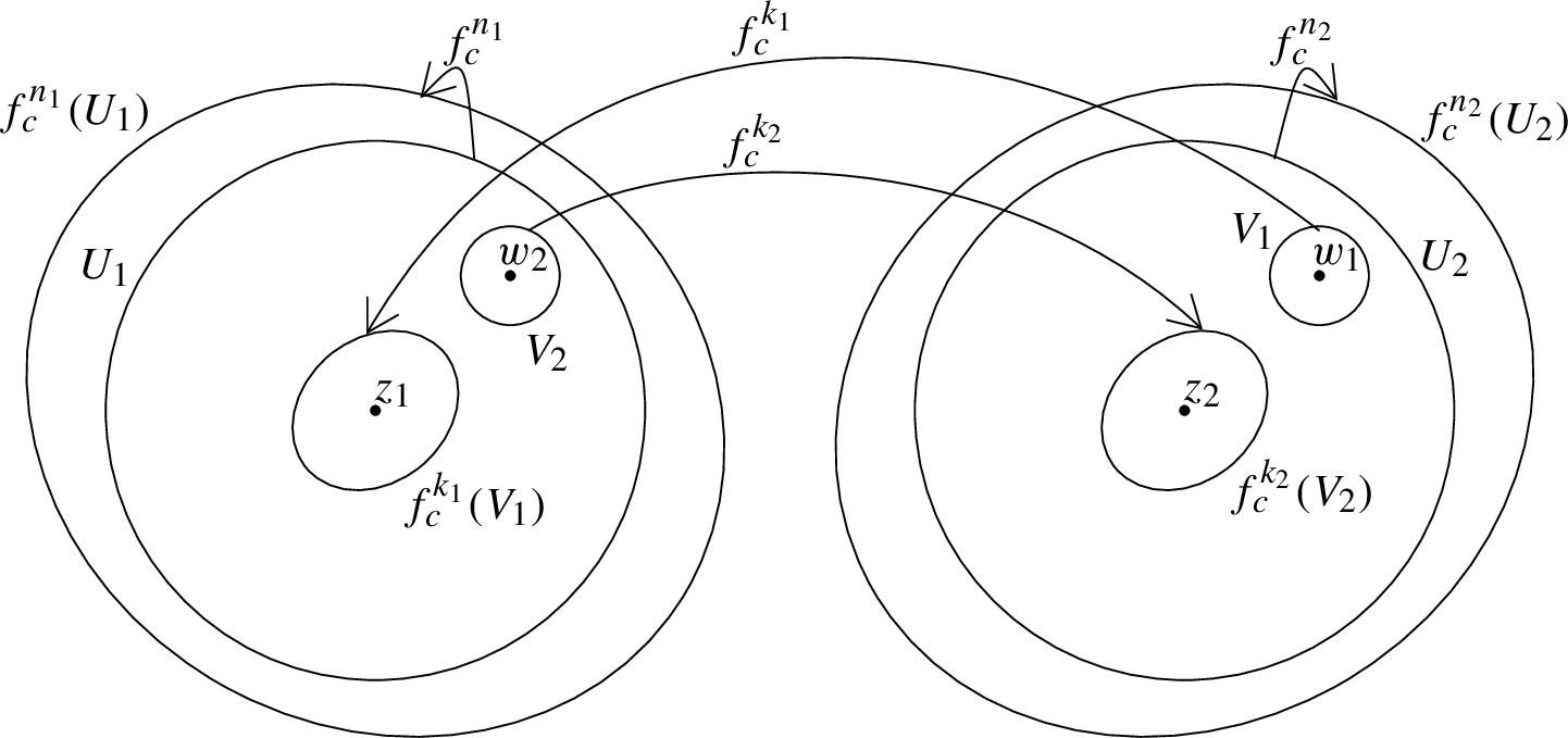
, the following hold (see Figure 2).
-
(a)
$f_{c}^{\circ k_{j}}$
is univalent on
$V_{j}$
and maps it inside
$U_{j}$
. -
(b) The neighborhood
$f_{c}^{\circ k_{j}}(V_{j})$
contains a repelling periodic point of period
$n_{j}$
for the map
$f_{c}$
. (For
$c=c_{0}$
, this periodic point is
$z_{j}$
, while for other
$c\in U$
, it is its perturbation.) -
(c) For any
$z\in V_{j}$
, we have (3)
$$ \begin{align} K^{-1}<\lvert (f_{c}^{\circ k_{j}})^{\prime}(z)\rvert <K. \end{align} $$


Maps and domains from the proof of Lemma 2.1.

For any
 $c\in U$
, let
 $\phi _{1,c}$
and
 $\phi _{2,c}$
be the inverse branches of
 $f_{c}^{n_{1}}$
and
 $f_{c}^{n_{2}}$
respectively, such that
 $\phi _{j,c}$
takes
 $U_{j}$
into itself for
 $j=1,2$
. Let
 $N\in {\mathbb {N}}$
be a sufficiently large number, such that for any
 $N_{1}, N_{2}\ge N$
and any
 $c\in U$
, we have
 $$ \begin{align} \phi_{1,c}^{\circ N_{1}} (V_{2}) \Subset f_{c}^{\circ k_{1}}(V_{1})\quad\text{and}\quad \phi_{2,c}^{\circ N_{2}} (V_{1}) \Subset f_{c}^{\circ k_{2}}(V_{2}). \end{align} $$
The existence of such a number N follows from property (b).
Assume
 $N_{1},N_{2}\in {\mathbb {N}}$
satisfy the condition
 $N_{1},N_{2}\ge N$
. Then for every
 $c\in U$
, one may consider the following composition of inverse branches of
 $f_{c}$
:
 $$ \begin{align*}V_{1}\xrightarrow{\enspace \phi_{2,c}^{\circ N_{2}} \enspace} f_{c}^{\circ k_{2}}(V_{2}) \xrightarrow{\enspace f_{c}^{\circ (-k_{2})} \enspace} V_{2} \xrightarrow{\enspace \phi_{1,c}^{\circ N_{1}} \enspace} f_{c}^{\circ k_{1}}(V_{1}) \xrightarrow{\enspace f_{c}^{\circ (-k_{1})} \enspace} V_{1}. \end{align*} $$
Let us denote this composition by
 $h_{c}\colon V_{1}\to V_{1}$
. By construction, this is a univalent map, and the inclusions (4) imply that
 $h_{c}(V_{1})\Subset V_{1}$
. Then, according to the Denjoy–Wolff theorem, the map
 $h_{c}$
has a unique fixed point
 $z_{c}$
in
 $V_{1}$
, which is a repelling periodic point of period
 $$ \begin{align*}M=n_{1}N_{1}+n_{2}N_{2}+k_{1}+k_{2} \end{align*} $$
for the map
 $f_{c}$
. Let
 $\mathcal O_{N_{1},N_{2}}$
denote the periodic orbit of this point when
 $c=c_{0}$
. Then the map
 $g_{\mathcal O_{N_{1},N_{2}}}$
is defined in U.
Consider the points
 $$ \begin{align*} z^{\prime}_{c} &= \phi_{2,c}^{\circ N_{2}}(z_{c})\,{\in}\, f_{c}^{\circ k_{2}}(V_{2}), \\ z^{\prime\prime}_{c} &= f_{c}^{\circ(-k_{2})}(z^{\prime}_{c})\,{\in}\, V_{2}, \\ z^{\prime\prime\prime}_{c} &= \phi_{1,c}^{\circ N_{1}}(z^{\prime\prime}_{c}) \,{\in}\, f_{c}^{\circ k_{1}}(V_{1}). \end{align*} $$
Then, using the chain rule, we get
 $$ \begin{align*} g_{\mathcal O_{N_{1},N_{2}}}(c) &= [(f_{c}^{\circ M})^{\prime}(z_{c})]^{1/M} \\[3pt] & = [(f_{c}^{\circ k_{1}})^{\prime}(z_{c})\cdot (f_{c}^{\circ (n_{1}N_{1})})^{\prime}(z^{\prime\prime\prime}_{c}) \cdot (f_{c}^{\circ k_{2}})^{\prime}(z^{\prime\prime}_{c}) \cdot (f_{c}^{\circ (n_{2}N_{2})})^{\prime}(z^{\prime}_{c})]^{1/M}. \end{align*} $$
After possibly shrinking the neighborhood U of
 $c_{0}$
, we may apply Proposition 2.3 for
 $V=U_{1}$
and
 $V=U_{2}$
. Then, the previous identity can be rewritten in the notation of Proposition 2.3 as
 $$ \begin{align} g_{\mathcal O_{N_{1},N_{2}}}(c)\! =\! [(f_{c}^{\circ k_{1}})^{\prime}(z_{c})]^{{1}/{M}}\!\cdot [h_{N_{1},z^{\prime\prime}_{c}}(c)]^{{n_{1}N_{1}}/{M}}\!\cdot [(f_{c}^{\circ k_{2}})^{\prime}(z^{\prime\prime}_{c})]^{{1}/{M}} \cdot [h_{N_{2}, z_{c}}(c)]^{{n_{2}N_{2}}/{M}}{.} \end{align} $$
Note that
 $z_{c}\in V_{1}$
,
 $z^{\prime \prime }_{c}\in V_{2}$
. Hence, applying inequality (3) and Proposition 2.3 to the identity (5), we conclude that if
 $N_{1},N_{2}\to \infty $
so that
 $$ \begin{align*}\frac{n_{1}N_{1}}{n_{1}N_{1}+n_{2}N_{2}}\to\alpha, \end{align*} $$
then
 $$ \begin{align} g_{\mathcal O_{N_{1},N_{2}}}(c) \to s\cdot (g_{\mathcal O_{1}}(c))^{\alpha} (g_{\mathcal O_{2}}(c))^{1-\alpha}, \end{align} $$
uniformly in
 $c\in U$
, for appropriate fixed branches of the degree maps
 $z\mapsto z^{\alpha }$
and
 $z\mapsto z^{1-\alpha }$
, and some constant
 $s\in {\mathbb {C}}$
, such that
 $\lvert s\rvert = 1$
.
Finally, the proof of Lemma 2.1 can be completed by taking logarithmic derivatives of both sides in equation (6) and applying Proposition 2.2.
3 The sets
$\mathcal Y_{c}$

We start this section by giving a proof of Theorem B. We note that our proof of part (ii) of Theorem B, providing the necessary and sufficient condition for
 $c\in {\mathbb {C}}\setminus {\mathbb M}$
to be contained in
 $\mathcal X$
, seriously depends on the assumption that
 $c\not \in {\mathbb M}$
. Furthermore, the condition itself seems to be wrong for some
 $c\in \partial {\mathbb M}$
, (cf. Remark 3.2). Indeed, the case
 $c\in {\mathbb M}$
appears to be more delicate. In the second part of this section, we provide a sufficient condition for
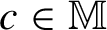 $c\in {\mathbb M}$
to be contained in
 $\mathcal X$
. Later, in §4.3, we show that this condition is satisfied for any
 $c\in {\mathbb M}$
.
3.1 Proof of Theorem B
To prove property (ii) of Theorem B, we need the following lemma.
Lemma 3.1. For any
 $c\in {\mathbb {C}}\setminus \partial {\mathbb M}$
, the family of maps
 $\{\nu _{\mathcal O}\mid \mathcal O\in \Omega _{c}\}$
is defined and is normal on any simply connected neighborhood
 $U\subset {\mathbb {C}}$
, such that
 $c\in U$
and
 ${U\cap \partial {\mathbb M}=\varnothing }$
. Furthermore, if
 $c\in {\mathbb {C}}\setminus {\mathbb M}$
, then the identical zero is not a limiting map of the normal family
 $\{\nu _{\mathcal O}\mid \mathcal O\in \Omega _{c}\}$
.
Proof. Fix
 $c\in {\mathbb {C}}\setminus \partial {\mathbb M}$
and a neighborhood U as in the statement of the lemma. Since
 $U\cap \partial {\mathbb M}=\varnothing $
, all repelling periodic orbits of
 $f_{c}$
remain to be repelling after analytic continuation in
 $c\in U$
. This implies that all maps from the family
 $$ \begin{align*} \mathcal G_{c}:=\{g_{\mathcal O}\mid \mathcal O\in\Omega_{c}\} \end{align*} $$
are defined in the neighborhood U and are analytic in it. (We recall that the maps
 $g_{\mathcal O}$
were defined in equation (2) and are appropriate branches of the roots of the multipliers.) Furthermore, for any
 $\tilde c\in U$
and
 $\mathcal O\in \Omega _{c}$
, we have
 $\lvert g_{\mathcal O}(\tilde c)\rvert \le 2\max _{z\in J_{\tilde c}}\lvert z\rvert = \mathrm {diam}(J_{\tilde c})$
, where
 $J_{\tilde c}$
is the Julia set of
 $f_{\tilde c}$
. Thus, the family
 $\mathcal G_{c}$
is locally uniformly bounded and hence normal in U. Since all maps from the family
 $\mathcal G_{c}$
are uniformly bounded away from zero, Proposition 2.2 implies normality of the family
 $\{\nu _{\mathcal O}\mid \mathcal O\in \Omega _{c}\}$
.
If
 $c\in {\mathbb {C}}\setminus {\mathbb M}$
, then without loss of generality we may assume that the domain U is simply connected and unbounded. Since for all
 $\tilde c\in {\mathbb {C}}$
sufficiently close to
 $\infty $
, the Julia set
 $J_{\tilde c}$
is contained in the annulus centered at zero with inner and outer radii being equal to
 $\sqrt {\lvert {\tilde c}\rvert }\pm 1$
, it follows that for every
 $\tilde c\in U$
sufficiently close to
 $\infty $
and for any
 $\mathcal O\in \Omega _{c}$
, we have
 $$ \begin{align} 2\sqrt{\lvert {\tilde c}\rvert}-2<\lvert g_{\mathcal O}(\tilde c)\rvert < 2\sqrt{\lvert {\tilde c}\rvert}+2, \end{align} $$
which implies that none of the limiting maps of the family
 $\mathcal G_{c}$
is a constant map. Then it follows that the identical zero is not a limiting map of the normal family
 $\{\nu _{\mathcal O}\mid \mathcal O\in \Omega _{c}\}$
.
Proof of Theorem B
First, we observe that property (i) of Theorem B is an immediate corollary from the averaging lemma (Lemma 2.1). Indeed, if
 $c\neq -2$
, then convexity of
 $\mathcal Y_{c}$
is obvious from Lemma 2.1. However, if
 $c=-2$
, then according to the same lemma, the set
 $\mathcal Y_{-2}$
is the union of a convex set and a single point
 $\nu _{\{2\}}(-2)$
, corresponding to the periodic orbit
 $\mathcal O=\{2\}$
. A direct computation shows that
 $$ \begin{align*}\rho_{\{2\}}(-2)= 4,\quad \rho_{\{2\}}^{\prime}(-2)= -2/3, \end{align*} $$
and hence
 $\nu _{\{2\}}(-2)=-1/6$
.
We proceed with the proof of part (ii) as follows: for
 $c\in {\mathbb {C}}\setminus {\mathbb M}$
, let U be a neighborhood of c that satisfies the conditions of Lemma 3.1. First, we observe that according to Lemma 3.1, the family
 $\{\nu _{\mathcal O}\mid \mathcal O\in \Omega _{c}\}$
, defined on U, is locally uniformly bounded, and hence the set
 $\mathcal Y_{c}$
is bounded.
Necessary condition for
 $c\in \mathcal X$
: If
 $c\in \mathcal X$
, then there exists a sequence of points
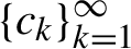 $\{c_{k}\}_{k=1}^{\infty }$
and a sequence of periodic orbits
 $\{\mathcal O_{k}\}_{k=1}^{\infty }\subset \Omega _{c}$
, such that
 $$ \begin{align*}\lim_{k\to\infty} c_{k} =c\quad\text{and}\quad \rho_{\mathcal O_{k}}^{\prime}(c_{k})=0\quad\text{for any } k\in{\mathbb{N}}. \end{align*} $$
According to Lemma 3.1, after extracting a subsequence, we may assume that the sequence of maps
 $\nu _{\mathcal O_{k}}$
converges to some holomorphic map
 $\nu \colon U\to {\mathbb {C}}$
uniformly on compact subsets of U. Since for any
 $k\in {\mathbb {N}}$
we have
 $\nu _{\mathcal O_{k}}(c_{k})=0$
, it follows by continuity that
 $\nu (c)=0$
. Finally, convergence of the maps
 $\nu _{\mathcal O_{k}}$
to
 $\nu $
implies that
 $$ \begin{align*}\lim_{k\to\infty}\nu_{\mathcal O_{k}}(c)=\nu(c)=0, \end{align*} $$
and hence
 $0\in \mathcal Y_{c}$
.
Sufficient condition for
 $c\in \mathcal X$
: However, if
 $0\in \mathcal Y_{c}$
, then either there exists a periodic orbit
 $\mathcal O\in \Omega _{c}$
, such that
 $\nu _{\mathcal O}(c)=0$
, or there exists a sequence of periodic orbits
 $\{\mathcal O_{k}\}_{k=1}^{\infty }\subset \Omega _{c}$
, such that
 $$ \begin{align*}\lim_{k\to\infty} \nu_{\mathcal O_{k}}(c)=0. \end{align*} $$
In the first case,
 $\rho _{\mathcal O}^{\prime }(c)=0$
, so
 $c\in \mathcal X$
according to Theorem 1.2.
In the second case, according to Lemma 3.1, after extracting a subsequence, we may assume that the sequence of maps
 $\nu _{\mathcal O_{k}}$
converges to some holomorphic map
 $\nu \colon U\to {\mathbb {C}}$
uniformly on compact subsets of U. By continuity, we have
 $\nu (c)=0$
, and, according to Lemma 3.1,
 $\nu \not \equiv 0$
. Then it follows from Rouché’s theorem that for any sufficiently large
 $k\in {\mathbb {N}}$
, there exists
 $c_{k}\in U$
, such that
 $\nu _{\mathcal O_{k}}(c_{k})=0$
and
 $\lim _{k\to \infty }c_{k}=c$
. The latter implies that
 $c\in \mathcal X$
, and completes the proof of Theorem B.
Remark 3.2. The above proof of part (ii) of Theorem B fails without the assumption
 $c\not \in {\mathbb M}$
. Indeed, if
 $c\in \partial {\mathbb M}$
, then the neighborhood U from Lemma 3.1 does not exist. Furthermore, even though
 $\partial {\mathbb M}\subset \mathcal X$
(since
 $\partial {\mathbb M}$
is the support of the bifurcation measure
 ${\mu _{\mathrm {bif}}}$
) and
 $-2\in \partial {\mathbb M}$
, the preliminary computations indicate that the set
 $\mathcal Y_{-2}$
seems to be disjoint from
 $0$
. In the case
 $c\in {\mathbb M}\setminus \partial {\mathbb M}$
, the above proof of the sufficient condition for
 $c\in \mathcal X$
fails since the limiting map
 $\nu $
might turn out to be the identical zero.
3.2 A sufficient condition for
$c\in {\mathbb M}$
to be contained in
$\mathcal X$


In this subsection, we prove the following sufficient condition for
 $c\in {\mathbb {C}}\setminus \{-2\}$
to be contained in
 $\mathcal X$
.
Lemma 3.3. Let
 $c\in {\mathbb {C}}\setminus \{-2\}$
be an arbitrary parameter. If there exist finitely many repelling periodic orbits
 $\mathcal O_{1},\mathcal O_{2},\ldots ,\mathcal O_{k}\in \Omega _{c}$
, such that
 $0$
is contained in the convex hull of the points
 $\nu _{\mathcal O_{1}}(c),\ldots , \nu _{\mathcal O_{k}}(c)$
, then
 $c\in \mathcal X$
.
When
 $c\in {\mathbb {C}}\setminus {\mathbb M}$
, the sufficient condition, given by Lemma 3.3, is an immediate corollary of Theorem B, but we will use Lemma 3.3 for
 $c\in {\mathbb M}\setminus \partial {\mathbb M}$
.
First, to prove Lemma 3.3, we need the following proposition.
Proposition 3.4. Let
 $c\in {\mathbb {C}}$
be an arbitrary parameter and let
 $\mathcal O_{1},\mathcal O_{2},\ldots ,\mathcal O_{k}\in \Omega _{c}$
be a finite collection of repelling periodic orbits. If
 $\alpha _{1},\ldots ,\alpha _{k}\in {\mathbb {R}}$
are such that
 ${\sum _{j=1}^{k}\alpha _{j}\neq 0}$
, then the map
 $$ \begin{align*}\nu:= \sum_{j=1}^{k}\alpha_{j}\nu_{\mathcal O_{j}}, \end{align*} $$
defined in a neighborhood of the point c, is not a constant map.
Proof. Since for every
 $j=1,\ldots ,k$
, the multipliers
 $\rho _{\mathcal O_{j}}$
are algebraic (multiple-valued) maps, it follows from equation (1) that the map
 $\nu $
has a single-valued meromorphic extension to any simply connected domain
 $U\subset {\mathbb {C}}$
that avoids finitely many branching points of the maps
 $\rho _{\mathcal O_{j}}$
. Note that none of the branching points lie on the real ray
 $(-\infty ,-3)$
, since
 $(-\infty ,-3)\cap {\mathbb M}=\varnothing $
. Furthermore, since for any parameter
 $\tilde c\in (-\infty ,-3)$
the corresponding Julia set
 $J_{\tilde c}$
lies on the real line, it follows that all maps
 $\rho _{\mathcal O_{j}}$
take real values when restricted to the ray
 $(-\infty ,-3)$
. Choose the domain U so that it is unbounded and
 $(-\infty ,-3)\subset U$
. Then for any
 $j=1,\ldots ,k$
, we have the same asymptotic relation
 $$ \begin{align*}\rho_{\mathcal O_{j}}(\tilde c)\sim \pm(-4\tilde c)^{\lvert {\mathcal O}_{j}\rvert/2}, \end{align*} $$
as
 $\tilde c\to -\infty $
within the domain U. A direct computation yields that
 $\nu _{\mathcal O_{j}}(\tilde c)\sim 1/(2\tilde c)$
, and hence
 $$ \begin{align*}\nu(\tilde c)\sim \frac{\sum_{j=1}^{k}\alpha_{j}}{2\tilde c}, \end{align*} $$
as
 $\tilde c\to -\infty $
within the domain U. Since
 $\sum _{j=1}^{k}\alpha _{j}\neq 0$
, the latter implies that
 $\nu $
is not a constant map.
Proof of Lemma 3.3
Since the convex hull of the points
 $\nu _{\mathcal O_{1}}(c),\ldots , \nu _{\mathcal O_{k}}(c)$
contains zero, it follows that there exist real non-negative constants
 $\alpha _{1},\ldots ,\alpha _{k}$
, such that
 $\sum _{j=1}^{k}\alpha _{j}=1$
and the analytic map
 $$ \begin{align*}\nu:= \sum_{j=1}^{k}\alpha_{j}\nu_{\mathcal O_{j}}, \end{align*} $$
defined in some neighborhood of the point c, satisfies
 $\nu (c)=0$
.
Since
 $c\neq -2$
, it follows from the averaging lemma (Lemma 2.1) that there exists a sequence of periodic orbits
 $\{\mathcal O_{m}^{\prime }\}_{m=1}^{\infty }\subset \Omega _{c}$
and a neighborhood
 $U\subset {\mathbb {C}}$
of the point c, such that all maps
 $\nu _{\mathcal O_{m}^{\prime }}$
are defined and analytic in U and
 $$ \begin{align*}\nu_{\mathcal O_{m}^{\prime}}\to\nu\quad\text{as }m\to\infty,\quad\text{uniformly on } U. \end{align*} $$
According to Proposition 3.4, the map
 $\nu $
is not the identical zero map. Now, since
 $\nu (c)=0$
, it follows from Rouché’s theorem that for any sufficiently large
 $m\in {\mathbb {N}}$
, the map
 $\nu _{\mathcal O_{m}^{\prime }}$
has a zero at some point
 $c_{m}\in U$
, and the points
 $c_{m}$
can be chosen so that
 $\lim _{m\to \infty }c_{m}=c$
. The latter implies that
 $c\in \mathcal X$
.
4 Proof of Theorem A
In this section, we complete the proof of Theorem A.
4.1 The set
$\mathcal X$
is bounded

First, we prove the following.
Lemma 4.1. The set
 $\mathcal X$
is bounded.
Proof. For a fixed parameter
 $c_{0}\in {\mathbb {C}}\setminus {\mathbb M}$
, the Julia set
 $J_{c_{0}}$
of the map
 $f_{c_{0}}$
is a Cantor set, and all periodic orbits of
 $f_{c_{0}}$
are repelling. For any periodic orbit
 $\mathcal O$
of
 $f_{c_{0}}$
, the locally defined map
 $g_{\mathcal O}$
can be extended by analytic continuation to an analytic map of a double cover of the complement of the Mandelbrot set
 ${\mathbb M}$
(see [Reference Firsova and Gorbovickis5, §4.1] for details). This means that if
 $$ \begin{align*}\phi_{\mathbb M}\colon{\mathbb{C}}\setminus{\mathbb M}\to{\mathbb{C}}\setminus\overline{{\mathbb{D}}} \end{align*} $$
is a fixed conformal diffeomorphism of
 ${\mathbb {C}}\setminus {\mathbb M}$
onto
 ${\mathbb {C}}\setminus \overline {{\mathbb {D}}}$
and
 $\unicode{x3bb} _{0}\in {\mathbb {C}}\setminus \overline {{\mathbb {D}}}$
is a fixed point, such that
 $\phi _{\mathbb M}^{-1}(\unicode{x3bb} _{0}^{2})=c_{0}$
, then the map
 $$ \begin{align*}\unicode{x3bb}\mapsto g_{\mathcal O}(\phi_{\mathbb M}^{-1}(\unicode{x3bb}^{2})), \end{align*} $$
defined for all
 $\unicode{x3bb} $
in a neighborhood of
 $\unicode{x3bb} _{0}$
, extends to a global holomorphic map
 $$ \begin{align*}\gamma_{\mathcal O}\colon {\mathbb{C}}\setminus\overline{{\mathbb{D}}}\to {\mathbb{C}}\setminus\overline{{\mathbb{D}}}. \end{align*} $$
Now assume that the statement of Lemma 4.1 does not hold. Then there exists a sequence of parameters
 $\{\unicode{x3bb} _{n}\}_{n\in {\mathbb {N}}}$
and a corresponding sequence of periodic orbits
 $\{\mathcal O_{n}\}_{n\in {\mathbb {N}}}$
, such that

Since the family of maps
 $\{\gamma _{\mathcal O}\}$
omits more than three points, which is normal by Montel’s theorem (cf. [Reference Firsova and Gorbovickis5, Lemma 4.7]), it follows that after extracting a subsequence, we may assume that the sequence of maps
 $\gamma _{\mathcal O_{n}}$
converges to a holomorphic map
 $\gamma \colon {\mathbb {C}}\setminus \overline {{\mathbb {D}}}\to {\mathbb {C}}\setminus \overline {{\mathbb {D}}}$
uniformly on compact subsets. Since for any
 $\tilde c\in {\mathbb {C}}$
sufficiently close to
 $\infty $
and any
 $\mathcal O\in \Omega _{c_{0}}$
inequality (7) holds, we conclude that
 $\gamma $
, as well as each
 $\gamma _{\mathcal O_{n}}$
, are non-constant maps that have a simple pole at infinity. However, equation (8) implies that
 $\gamma $
has at least a double pole at infinity, which provides a contradiction.
Next, we proceed with proving the remaining statements of Theorem A.
4.2 The set
$\mathcal X\setminus {\mathbb M}$

First we study the set
 $\mathcal X\setminus {\mathbb M}$
, that is, the portion of the set
 $\mathcal X$
that is contained in the complement of the Mandelbrot set. We note that even though numerical computations from [Reference Belova and Gorbovickis1], together with Theorem 1.2, suggest that this set is non-empty, a rigorous computer-free proof of this fact has not been provided so far. We fill this gap by proving the following lemma.
Lemma 4.2. The set
 $\mathcal X\setminus {\mathbb M}$
has non-empty interior.
The idea of the proof of Lemma 4.2 is to show that the sufficient condition from Lemma 3.3 is satisfied for all c in a neighborhood of the parabolic parameter
 $c_{0}=-3/4$
. The rest of the proof is technical. We will need explicit formulas for the maps
 $\nu _{\mathcal O}$
, corresponding to periodic orbits
 $\mathcal O$
of periods
 $1$
,
 $2$
, and
 $3$
.
Proposition 4.3. Let
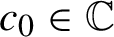 $c_{0}\in {\mathbb {C}}$
and a corresponding periodic orbit
 $\mathcal O$
of
 $f_{c_{0}}$
be such that the map
 $\nu := \nu _{\mathcal O}$
is defined in a neighborhood of the point
 $c=c_{0}$
. Then the following holds.
-
(i) If
$\lvert {\mathcal O}\rvert = 1$
, then where the two branches of the root correspond to the two different periodic orbits of period
$$ \begin{align*}\nu(c) = \frac{2}{4c-1-\sqrt{1-4c}}, \end{align*} $$
$1$
.
-
(ii) If
$\lvert {\mathcal O}\rvert = 2$
, then
$$ \begin{align*}\nu(c) = \frac{1}{2c+2}. \end{align*} $$
-
(iii) If
$\lvert {\mathcal O}\rvert = 3$
, then where the two branches of the root correspond to the two different periodic orbits of period
$$ \begin{align*}\nu(c) = \frac{12c^{3}+37c^{2}+32c+7 -(c^{2}+6c+7)\sqrt{-4c-7}}{6(4c+7)(c^{3}+2c^{2}+c+1)}, \end{align*} $$
$3$
.


Proof. When
 $\lvert {\mathcal O}\rvert = 1$
, that is,
 ${\mathcal O}$
is a fixed point z, solving the equation
 $f_{c}(z)=z$
yields
 $$ \begin{align*}\rho_{c_{0},\mathcal O}(c) = 2z=1+\sqrt{1-4c}. \end{align*} $$
Then after a direct computation, we get
 $$ \begin{align*}\nu(c) = \frac{\rho_{c_{0},\mathcal O}^{\prime}(c)}{\rho_{c_{0},\mathcal O}(c)} = \frac{2}{4c-1-\sqrt{1-4c}}. \end{align*} $$
When
 $\lvert {\mathcal O}\rvert = 2$
, there is only one periodic orbit of period
 $2$
. Its multiplier is the free term of the polynomial
 $$ \begin{align*}p(z)=\frac{4(f_{c}^{\circ 2}(z)-z)}{f_{c}(z)-z}=4z^{2}+4z+4(c+1). \end{align*} $$
Now, a direct computation yields the formula for
 $\nu (c)$
in part (ii) of the proposition.
Finally, in the case
 $\lvert {\mathcal O}\rvert = 3$
, there are two periodic orbits of period
 $3$
and according to [Reference Stephenson11], the multiplier
 $\rho =\rho (c)$
of each of these orbits satisfies the equation
 $$ \begin{align*}c^{3}+2c^{2}+(1-\rho/8)c+(1-\rho/8)^{2}=0. \end{align*} $$
After solving this equation for
 $\rho $
, we obtain
 $$ \begin{align*}\rho(c) = 8+4c-4c\sqrt{-4c-7}. \end{align*} $$
Then a direct computation yields the formula for
 $\nu (c)$
in part (iii) of the proposition.
Proof of Lemma 4.2
We consider the maps
 $\nu _{\mathcal O}$
in a neighborhood of the point
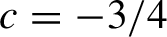 $c=-3/4$
for periodic orbits
 $\mathcal O$
of periods
 $1$
,
 $2$
, and
 $3$
. The parameter
 $c=-3/4$
is the point at which the hyperbolic component of period
 $2$
touches the main cardioid of the Mandelbrot set. In particular, all considered functions are defined and analytic in a neighborhood U of that point.
For each
 $c\in U$
, let
 $H_{c}$
denote the convex hull of the finite set
 $\{\nu _{\mathcal O}(c)\mid \lvert {\mathcal O}\rvert = 1, 2, 3\}$
. It follows from Proposition 4.3 that
 $\nu _{\mathcal O}(-3/4)$
is equal to:
-
•
$-1$
or
$-1/3$
, when
$\lvert {\mathcal O}\rvert =1$
; -
•
$2$
, when
$\lvert {\mathcal O}\rvert =2$
; -
•
$- {10}/{183} \pm ({49}/{183})i$
, when
$\lvert {\mathcal O}\rvert =3$
;


and hence
 $H_{-3/4}$
contains
 $0$
in its interior. By continuity, it follows that the convex hull
 $H_{c}$
contains
 $0$
for all c in some open complex neighborhood V of the point
 $-3/4$
. Since
 $c=-3/4$
is a parabolic parameter, it follows that
 $V\setminus {\mathbb M}$
is a nonempty open set. According to Lemma 3.3, we observe that
 $V\setminus {\mathbb M}\subset \mathcal X$
, which completes the proof of Lemma 4.2.
Next, we prove the following lemma.
Lemma 4.4. For any point
 $c_{0}\in \mathcal X\setminus {\mathbb M}$
, there exists a continuous path
 $\gamma \colon [0,1]\to {\mathbb {C}}$
, such that
 $\gamma (0)=c_{0}$
,
 $\gamma ([0,1))\subset \mathcal X\setminus {\mathbb M}$
, and
 $\gamma (1)\in \partial {\mathbb M}$
.
Proof.
Step 1: First, we prove this lemma under the assumption that
 $c_{0}\in \mathcal X\setminus {\mathbb M}$
is such that there exists a periodic orbit
 $\mathcal O$
of the map
 $f_{c_{0}}$
, for which
 $\nu _{\mathcal O}(c_{0})=0$
. We fix this periodic orbit
 $\mathcal O$
and let
 $\mathcal O_{2}$
be the unique periodic orbit of period
 $2$
for the map
 $f_{c_{0}}$
. Note that according to Proposition 4.3, we have
 $\nu _{\mathcal O_{2}}\neq 0$
, and hence
 $\mathcal O\neq \mathcal O_{2}$
. Then for each
 $t\in {\mathbb {R}}$
, we consider the map
 $$ \begin{align} \nu_{t}:=(1-t)\nu_{\mathcal O}+ t\nu_{\mathcal O_{2}}, \end{align} $$
defined in a neighborhood of the point
 $c_{0}$
.
Observe that for each
 $t\in {\mathbb {R}}$
, the map
 $\nu _{t}$
extends to a multiple valued algebraic map. The set of all poles and branching points of
 $\nu _{t}$
is contained in a finite set
 $Q\subset {\mathbb {C}}$
, which is the union of all poles and branching points of the two (global) multiple valued algebraic maps
 $\nu _{\mathcal O}$
and
 $\nu _{\mathcal O_{2}}$
. Since these points are some parabolic parameters and centers of appropriate hyperbolic components, it follows that the set Q is contained in
 ${\mathbb M}$
. Moreover, the set Q is independent of t.
According to Proposition 3.4, for any
 $t\in {\mathbb {R}}$
, the map
 $\nu _{t}$
is not identically zero, and hence for any
 $c\in {\mathbb {C}}\setminus Q$
,
 $t_{0}\in {\mathbb {R}}$
and a branch
 $\tilde \nu _{t_{0}}$
of
 $\nu _{t_{0}}$
, such that
 $\tilde \nu _{t_{0}}(c)=0$
, there exists a continuous (not necessarily unique) local curve
 $t\mapsto c(t)$
, defined for t in a neighborhood of
 $t_{0}$
and satisfying
 $\tilde \nu _{t}(c(t))=0$
and
 $c(t_{0})= c$
, where
 $\tilde \nu _{t}$
is a branch of
 $\nu _{t}$
that is a local perturbation of
 $\tilde \nu _{t_{0}}$
. (If
 $\tilde \nu _{t_{0}}^{\prime }(c)=0$
, then there can be finitely many such local curves.) We observe that any such curve (that is, the image of the map c) that lies outside of
 ${\mathbb M}$
is contained in
 $\mathcal X$
. Indeed, for each t, the branch
 $\tilde \nu _{t}$
, satisfying
 $\tilde \nu _{t}(c(t))=0$
, can be represented locally as
 $\tilde \nu _{t} = (1-t)\nu _{\tilde {\mathcal O}}+t\nu _{\mathcal O_{2}}$
, where
 $\tilde {\mathcal O}$
is a periodic orbit of
 $f_{c(t)}$
, obtained as analytic continuation of the orbit
 $\mathcal O$
. Hence, it follows from part (i) of Theorem B that
 $0\in \mathcal Y_{c(t)}$
and then part (ii) of Theorem B implies that
 $c(t)\in \mathcal X$
.
We apply the above observation in the case of
 $c = c_{0}$
and
 $t_{0}=0$
and let
 $\tilde c\colon [0,s)\to {\mathbb {C}}\setminus {\mathbb M}$
be a maximal continuous curve satisfying the following conditions:
-
(i)
$s\in (0,+\infty ]$
; -
(ii)
$\tilde c(0)=c_{0}$
, and for any
$t\in [0,s)$
we have
$\nu _{t}(\tilde c(t))=0$
, where
$\nu _{t}$
is viewed as the analytic continuation of the local map of equation (9) along the curve
$\tilde c$
from
$\tilde c(0)$
to a neighborhood of
$\tilde c(t)$
.


(Here, ‘maximal’ means that there is no other curve
 $\hat c$
in
 ${\mathbb {C}}\setminus {\mathbb M}$
, satisfying the same two properties, and defined on a longer interval
 $[0,\hat s)\supsetneq [0,s)$
, so that
 $\hat c(t)=\tilde c(t)$
for any
 $t\in [0,s)$
.)
First, it follows from Proposition 4.3 that the map
 $\nu _{1}=\nu _{\mathcal O_{2}}$
does not vanish on
 ${\mathbb {C}}$
, and hence
 $s\le 1$
. We want to show that the limit
 $$ \begin{align*}\lim_{t\to s^{-}}\,\tilde c(t) \end{align*} $$
exists and is finite. The above discussion implies that
 $\tilde c([0,s))\subset \mathcal X$
, and hence according to Lemma 4.1, the set
 $\tilde c([0,s))$
is bounded, thus,
 $\tilde c(t)$
accumulates on some bounded set A as
 $t\to s^{-}$
. Let
 $c_{1}\in A$
be an arbitrary limit point of
 $\tilde c(t)$
as
 $t\to s^{-}$
. Then since the branches of
 $\nu _{t}$
converge to the corresponding branches of
 $\nu _{s}$
uniformly on compact subsets of
 ${\mathbb {C}}\setminus Q$
, it follows that either
 $c_{1}\in Q$
or
 $\tilde \nu _{s}(c_{1})=0$
for some branch
 $\tilde \nu _{s}$
of
 $\nu _{s}$
. Since both the set Q and the set of zeros of a (global) algebraic map
 $\nu _{s}$
are finite sets, it follows that A is a discrete set. Finally, since
 $\tilde c$
is a continuous function, the set A must be connected, and hence consists of a single point. This implies that the limit
 $\lim _{t\to s^{-}}\tilde c(t)$
exists, and the curve
 $\tilde c$
extends continuously to the closed interval
 $[0,s_{0}]$
.
Now the proof of Step 1 can be completed by observing that
 $\tilde c(s)\in \partial {\mathbb M}$
, because otherwise, if
 $\tilde c(s)\in {\mathbb {C}}\setminus {\mathbb M}$
, then
 $\tilde c(s)\not \in Q$
and the curve
 $\tilde c$
can be continued beyond the parameter s; hence,
 $\tilde c$
is not maximal. The required curve
 $\gamma $
is obtained from the curve
 $\tilde c|_{[0,s]}$
by an appropriate reparameterization.
Step 2: Now we assume that the point
 $c_{0}\in \mathcal X\setminus {\mathbb M}$
is not a critical point of the multiplier of any periodic orbit. Our goal is to show that there is a path that lies in
 $\mathcal X\setminus {\mathbb M}$
and joins
 $c_{0}$
with a critical point of the multiplier of some periodic orbit. Together with Step 1, this will complete the proof of the lemma.
Note that since
 $c_{0}\in \mathcal X\setminus {\mathbb M}$
, there exists a sequence of periodic orbits
 $\{\mathcal O_{j}\}_{j\in {\mathbb {N}}}$
of
 $f_{c_{0}}$
and a sequence of parameters
 $\{c_{j}\}_{j\in {\mathbb {N}}}\subset {\mathbb {C}}\setminus {\mathbb M}$
, such that
 $\lim _{j\to \infty }c_{j}=c_{0}$
, and for each
 $j\in {\mathbb {N}}$
, we have
 $\nu _{\mathcal O_{j}}(c_{j})=0$
.
Fix an arbitrary simply connected open domain
 $V\Subset {\mathbb {C}}\setminus {\mathbb M}$
, such that
 $c_{0}\in V$
. Since algebraic extensions of the local maps
 $\nu _{\mathcal O_{j}}$
do not have branching points outside
 ${\mathbb M}$
, it follows that each of the maps
 $\nu _{\mathcal O_{j}}$
has an analytic extension to the domain V. For the rest of the proof, we will identify the maps
 $\nu _{\mathcal O_{j}}$
with these analytic extensions. According to Lemma 3.1, the family of maps
 $\{\nu _{\mathcal O_{j}}\}_{j\in {\mathbb {N}}}$
is normal in V, so after extracting a subsequence, we may assume that the sequence of maps
 $\{\nu _{\mathcal O_{j}}\}_{j\in {\mathbb {N}}}$
converges to some analytic map
 $\nu \colon V\to {\mathbb {C}}$
uniformly on compact subsets of V. By continuity, it follows that
 $\nu (c_{0})=0$
. However, Lemma 3.1 implies that the map
 $\nu $
is not an identical zero, and hence
 $c_{0}$
is an isolated zero of the map
 $\nu $
.
Consider a neighborhood
 $U\Subset V$
, such that
 $c_{0}\in U$
and
 $\nu $
does not vanish on the boundary
 $\partial U$
. Let
 $r\in {\mathbb {R}}$
be defined as
 $$ \begin{align} r:= \min_{z\in\partial U} \lvert \nu(z)\rvert>0. \end{align} $$
Then there exists
 $N\in {\mathbb {N}}$
, such that for any
 $j\ge N$
, we have
 $$ \begin{align} \max_{z\in\overline U} \lvert \nu(z)-\nu_{j}(z)\rvert < r/2. \end{align} $$
For each
 $t\in [0,1]$
, consider the map
 $$ \begin{align*}\nu_{t}:= (1-t)\nu+t\nu_{\mathcal O_{N}}, \end{align*} $$
which, by construction, is defined and analytic in V. Similarly to the proof of Step 1, there exist
 $s\in (0,1]$
and a maximal continuous curve
 $\tilde c\colon [0,s)\to V$
, such that
 $\tilde c(0)=c_{0}$
and
 $\nu _{t}(\tilde c(t))=0$
for any
 $t\in [0,s)$
. Conditions (10) and (11) imply that for each
 $t\in [0,1]$
, the map
 $\nu _{t}$
does not vanish at any point of
 $\partial U$
, and hence
 $\tilde c([0,s))\subset U$
. In particular, the image
 $\tilde c([0,s))$
is bounded, and the same argument as in Step 1 implies that the map
 $\tilde c$
extends continuously to the parameter
 $t=s$
. Since
 $\nu _{t}\to \nu _{s}$
uniformly in U as
 $t\to s$
and
 $\nu _{s}$
does not vanish on
 $\partial U$
, it follows that
 $\nu _{s}(\tilde c(s))=0$
and
 $\tilde c(s)\in U$
. Finally, since
 $U\subset {\mathbb {C}}\setminus {\mathbb M}$
, maximality of the curve
 $\tilde c$
implies that
 $s=1$
, and thus the curve
 $\tilde c$
connects the point
 $c_{0}=\tilde c(0)$
with a point
 $\tilde c(1)$
, which is a zero of the function
 $\nu _{\mathcal O_{N}}$
.
To complete the proof of the lemma, we will show that the curve
 $\tilde c([0,1])$
lies in
 $\mathcal X\setminus {\mathbb M}$
. Observe that for each
 $t\in [0,1]$
, the sequence of maps
 $\nu _{t,j} = (1-t)\nu _{\mathcal O_{j}}+t\nu _{\mathcal O_{N}}$
converges to
 $\nu _{t}$
uniformly in
 $\overline U$
as
 $j\to \infty $
. Therefore, for all sufficiently large
 $j\in {\mathbb {N}}$
, there exists a point
 $c_{t,j}\in U$
, such that
 $$ \begin{align*}\nu_{t,j}(c_{t,j})=0\quad\text{and}\quad c_{t,j}\to\tilde c(t)\quad\text{as }j\to\infty. \end{align*} $$
The first condition together with both parts of Theorem B implies that
 $c_{t,j}\in \mathcal X\setminus {\mathbb M}$
for all sufficiently large j. Finally, since the set
 $\mathcal X$
is closed, it follows from the second condition that
 $\tilde c(t)\in \mathcal X\setminus {\mathbb M}$
, which completes the proof of the lemma.
4.3 The set
$\mathcal X\cap {\mathbb M}$

Here we turn to the study of the portion of the set
 $\mathcal X$
that is contained in the Mandelbrot set. We show that the whole Mandelbrot set is contained in
 $\mathcal X$
.
Lemma 4.5. The inclusion
 ${\mathbb M}\subset \mathcal X$
holds.
Before proving Lemma 4.5, we need several additional results.
For any
 $c\in {\mathbb {C}}$
and any
 $k\in {\mathbb {N}}$
, let
 $\Omega _{c}^{k}$
be the set of all periodic orbits of period k for the map
 $f_{c}$
. (In particular,
 $\Omega _{c}^{k}$
may contain a non-repelling orbit, if it exists.)
Lemma 4.6. Let
 $c_{0}\in {\mathbb {C}}$
be an arbitrary parameter that is neither parabolic nor critically periodic. Then for any
 $k\in {\mathbb {N}}$
, and the corresponding function
 $F_{k}(c):= f_{c}^{\circ (k-1)}(c)$
, the following holds:
 $$ \begin{align} \frac{F_{k}^{\prime}(c_{0})}{kF_{k}(c_{0})} = \sum_{m\in{\mathbb{N}}, m|k}\,\,\sum_{\mathcal O\in\Omega_{c_{0}}^{m}}\frac{m}{k}\nu_{\mathcal O}(c_{0}), \end{align} $$
where the summation goes over all
 $m\in {\mathbb {N}}$
, such that m divides k, and over all periodic orbits
 $\mathcal O\in \Omega _{c_{0}}^{m}$
.
Proof. For every
 $k\in {\mathbb {N}}$
, it follows from Vieta’s formulas that
 $F_{k}(c_{0})$
is the product of all fixed points of the map
 $f_{c_{0}}^{\circ k}$
, counted with multiplicities. Since
 $c_{0}$
is a non-parabolic parameter, all of these fixed points have multiplicity one, and hence we have
 $$ \begin{align} F_{k}(c_{0}) = 2^{-2^{k}}\prod_{m\in{\mathbb{N}}, m|k}\,\,\prod_{\mathcal O\in\Omega_{c_{0}}^{m}}\rho_{\mathcal O}(c_{0}). \end{align} $$
Since the parameter
 $c_{0}$
is not critically periodic, we have
 $F_{k}(c_{0})\neq 0$
, and for any periodic orbit
 $\mathcal O$
of
 $f_{c_{0}}$
, the map
 $\nu _{\mathcal O}$
is defined and analytic in some fixed neighborhood of the point
 $c_{0}$
. This implies that both the left hand side and the right hand side of equation (12) are defined. Finally, the identity (12) can be obtained from equation (13) by a direct computation.
Next, we prove a slightly refined version of the averaging lemma.
Proposition 4.7. Under the conditions of Lemma 2.1, if the periods of the periodic orbits
 $\mathcal O_{1}$
and
 $\mathcal O_{2}$
are relatively prime, then the sequence of repelling periodic orbits
 $\{\mathcal O_{j}\}_{j=3}^{\infty }$
from Lemma 2.1 can be chosen so that
 $\lvert {\mathcal O}_{j}\rvert = j$
for any
 $j\ge 3$
.
Proof. Here we refer to the proof of the averaging lemma (Lemma 2.1). Define
 $n_{1}:= \lvert {\mathcal O}_{1}\rvert $
and
 $n_{2}:= \lvert {\mathcal O}_{2}\rvert $
. It was shown that there exist constants
 $k_{1}, k_{2}\in {\mathbb {N}}$
(that depend on
 $c_{0}$
,
 $\mathcal O_{1}$
, and
 $\mathcal O_{2}$
), such that the sequence of orbits
 $\{\mathcal O_{j}\}_{j=3}^{\infty }$
can be chosen to satisfy the following:
 $$ \begin{align*} \lvert {\mathcal O}_{j}\rvert = n_{1}N_{1,j}+n_{2}N_{2,j}+k_{1}+k_{2}, \end{align*} $$
for some
 $N_{1,j},N_{2,j}\in {\mathbb {N}}$
, where
 $$ \begin{align} N_{1,j},N_{2,j}\to\infty\quad\text{and}\quad\frac{n_{1}N_{1,j}}{n_{1}N_{1,j}+n_{2}N_{2,j}}\to\alpha\quad\text{as }j\to\infty. \end{align} $$
To prove the proposition, it is sufficient to show that for every
 $\alpha \in [0,1]$
, there exist two sequences
 $\{N_{1,j}\}_{j=3}^{\infty }$
,
 $\{N_{2,j}\}_{j=3}^{\infty }$
of positive integers that satisfy condition (14) and such that
 $$ \begin{align*}j=n_{1}N_{1,j}+n_{2}N_{2,j}+k_{1}+k_{2} \end{align*} $$
for all sufficiently large
 $j\in {\mathbb {N}}$
.
It follows from elementary number theory that for every sufficiently large
 $j\in {\mathbb {N}}$
, the Diophantine equation
 $$ \begin{align} j=n_{1}N_{1}+n_{2}N_{2}+k_{1}+k_{2} \end{align} $$
has a solution
 $(N_{1}, N_{2})=(K_{1}, K_{2})\in {\mathbb {N}}^{2}$
in positive integers. Furthermore, the set of all pairs
 $(N_{1},N_{2})\in {\mathbb {N}}^{2}$
, satisfying condition (15), can be described as
 $$ \begin{align*}\mathcal N_{j} = \{(K_{1}-sn_{2}, K_{2}+sn_{1})\mid s\in{\mathbb{Z}},\quad\text{and}\quad K_{1}-sn_{2}, K_{2}+sn_{1}>0\}, \end{align*} $$
so the set of all fractions
 $$ \begin{align*}\frac{n_{1}N_{1}}{n_{1}N_{1}+n_{2}N_{2}}=\frac{n_{1}N_{1}}{j-k_{1}-k_{2}}, \end{align*} $$
such that
 $(N_{1},N_{2})\in \mathcal N_{j}$
, will consist of the real number
 $n_{1}N_{1}/(j-k_{1}-k_{2})$
and all other rational numbers from
 $(0,1)$
that differ from the first number by an integer multiple of
 $\theta _{j}=n_{1}n_{2}/(j-k_{1}-k_{2})$
. Now, since
 $\theta _{j}\to 0$
as
 $j\to \infty $
, it follows that for every sufficiently large
 $j\in {\mathbb {N}}$
, one can choose a pair
 $(N_{1,j},N_{2,j})\in \mathcal N_{j}$
so that condition (14) holds.
Proof of Lemma 4.5
First, observe that Theorem 1.1 and the fact that
 $\sup ({\mu _{\mathrm {bif}}})=\partial {\mathbb M}$
imply the inclusion
 $\partial {\mathbb M}\subset \mathcal X$
. Thus, we only need to show that the interior of
 ${\mathbb M}$
is contained in
 $\mathcal X$
. Let
 $c_{0}\in {\mathbb M}$
be a non-critically periodic interior point of the Mandelbrot set. We note that
 $c_{0}$
belongs to either a hyperbolic or a queer component, in case if the latter ones exist. For each
 $k\in {\mathbb {N}}$
, consider the map
 $F_{k}\colon {\mathbb {C}}\to {\mathbb {C}}$
defined by the formula
 $$ \begin{align*}F_{k}(c):= f_{c}^{\circ(k-1)}(c). \end{align*} $$
Since
 $c_{0}\in {\mathbb M}$
, the sequence
 $\{F_{k}(c_{0})\}_{k=1}^{\infty }$
is bounded, and hence there exists a subsequence
 $\{k_{m}\}_{m\in {\mathbb {N}}}\subset {\mathbb {N}}$
, such that the limit
 $\lim _{m\to \infty } F_{k_{m}}(c_{0})$
exists and is equal to some number
 $w\in {\mathbb {C}}$
. We may assume that
 $w\neq 0$
. Otherwise, if
 $w=0$
, then take the subsequence
 $\{k_{m}+1\}_{m\in {\mathbb {N}}}$
instead of the subsequence
 $\{k_{m}\}_{m\in {\mathbb {N}}}$
. Since
 $c_{0}$
is an interior point of
 ${\mathbb M}$
, the family of maps
 $\{F_{k_{m}}\}_{m\in {\mathbb {N}}}$
is normal, when restricted to some open neighborhood U of
 $c_{0}$
, so after further extracting a subsequence, we may assume that the sequence of functions
 $\{F_{k_{m}}\}_{m\in {\mathbb {N}}}$
converges to some holomorphic function
 $F\colon U\to {\mathbb {C}}$
on compact subsets of U.
Let us assume that
 $c_{0}\not \in \mathcal X$
. Then, according to Lemma 3.3, there exists a closed half-plane
 $H\subset {\mathbb {C}}$
such that
 $0\in \partial H$
and for any repelling periodic orbit
 $\mathcal O\in \Omega _{c_{0}}$
, we have
 $\nu _{\mathcal O}(c_{0})\in H$
. For any
 $z\in H$
, let
 ${\operatorname {dist}}(z,\partial H)$
denote the Euclidean distance from z to the boundary line
 $\partial H$
of H. Then, under the above assumption, the following holds.
Proposition 4.8. Assume the set
 ${\mathbb M}\setminus \mathcal X$
is nonempty and
 $c_{0}\in {\mathbb M}\setminus \mathcal X$
. Let the half-plane H and the sequence
 $\{k_{m}\}_{m\in {\mathbb {N}}}$
be the same as above. Then for any
 $\varepsilon>0$
, there exists
 $M=M(\varepsilon )\in {\mathbb {N}}$
such that for any
 $m\ge M$
and any periodic orbit
 $\mathcal O\in \Omega _{c_{0}}$
of period
 $\lvert {\mathcal O}\rvert =k_{m}$
, the inequality
 $$ \begin{align*}{\operatorname{dist}}(\nu_{\mathcal O}(c_{0}),\partial H)<\varepsilon \end{align*} $$
holds.
Proof. According to Lemma 4.6,
 $$ \begin{align*} \lim_{m\to\infty} \sum_{j\in{\mathbb{N}}, j|k_{m}}\,\,\sum_{\mathcal O\in\Omega_{c_{0}}^{j}}\frac{j}{k_{m}}\nu_{\mathcal O}(c_{0}) = \lim_{m\to\infty} \frac{F_{k_{m}}^{\prime}(c_{0})}{k_{m}F_{k_{m}}(c_{0})} = \lim_{m\to\infty} \frac{F^{\prime}(c_{0})}{k_{m}w}=0, \end{align*} $$
where F is the limiting map of the sequence of maps
 $\{F_{k_{m}}\}_{m\in {\mathbb {N}}}$
, and
 $w=F(c_{0})\neq 0$
. Note that for all but possibly one non-repelling orbit
 $\hat {\mathcal O}$
of fixed period
 $\hat j$
, the terms in the above summation belong to H. As
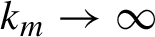 $k_{m}\to \infty $
, the contribution
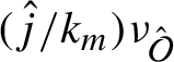 $({\hat j}/{k_{m}})\nu _{\hat {\mathcal O}}$
of this non-repelling orbit in the summation goes to zero. Then it follows that
 $$ \begin{align*} \lim_{m\to\infty} {\operatorname{dist}}\bigg(\sum_{\mathcal O\in\Omega_{c_{0}}^{k_{m}}}\nu_{\mathcal O}(c_{0}),\,\, \partial H\bigg) =0, \end{align*} $$
which implies Proposition 4.8.
Finally, we complete the proof of Lemma 4.5 by observing that under the above assumption where
 $c_{0}\not \in \mathcal X$
, according to Lemma 3.3, the half-plane H can be chosen so that for at least one repelling periodic orbit
 $\mathcal O_{1}\in \Omega _{c_{0}}$
, the value
 $\nu _{\mathcal O_{1}}(c_{0})$
lies in the interior of H. Let
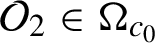 $\mathcal O_{2}\in \Omega _{c_{0}}$
be any other repelling periodic orbit whose period is relatively prime to the period of
 $\mathcal O_{1}$
. Then, according to Lemma 2.1 and Proposition 4.7 with the parameter
 $\alpha $
fixed at
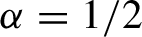 $\alpha =1/2$
, it follows that for each sufficiently large
 $m\in {\mathbb {N}}$
, there exists a periodic orbit
 $\mathcal O\in \Omega _{c_{0}}$
of period
 $k_{m}$
, such that
 $$ \begin{align*}{\operatorname{dist}}(\nu_{\mathcal O}(c_{0}),\partial H)> \tfrac{1}{3}{\operatorname{dist}}(\nu_{\mathcal O_{1}}(c_{0}),\partial H). \end{align*} $$
The latter contradicts Proposition 4.8, and hence the assumption
 $c_{0}\not \in \mathcal X$
was false. Since
 $c_{0}$
was an arbitrary non-critically periodic parameter from the interior of
 ${\mathbb M}$
, and critically periodic parameters form a nowhere dense subset of
 ${\mathbb M}$
, this completes the proof of Lemma 4.5.
Proof of Theorem A
The proof is a combination of several lemmas. We have
 ${\mathbb M}\subset \mathcal X$
due to Lemma 4.5. The set
 $\mathcal X$
is bounded according to Lemma 4.1. From Lemmas 4.4 and 4.5, it follows that the set
 $\mathcal X$
is connected. Finally, Lemma 4.2 implies that the set
 $\mathcal X\setminus {\mathbb M}$
has nonempty interior.
Remark 4.9. We note that Lemmas 4.4 and 4.5 would imply path connectedness (instead of just connectedness) of the set
 $\mathcal X$
if the MLC conjecture holds. At the same time, it seems that the MLC conjecture is much stronger than the conjecture that the set
 $\mathcal X$
is path connected. For example, the latter conjecture could be established without the MLC, if one can improve Lemma 4.5 by showing that there is a Jordan domain
 $U\subset {\mathbb {C}}$
such that
 ${\mathbb M}\subset \overline U\subset \mathcal X$
. Figure 1 and the discussion in Appendix A suggest that computer-assisted methods can be used in the attempt to construct such a domain U.
Acknowledgements
Research of T.F. was supported in part by NSF grant DMS-1505342, and by Laboratory of Dynamical Systems and Applications NRU HSE, Grant Agreement No. 075-15-2019-1931. Research of I.G. was partially supported by the Deutsche Forschungsgemeinschaft (DFG, German Research Foundation)—project number 455038303. We also thank the anonymous referee for valuable comments and suggestions.
A Appendix. Pictures
Theorems A and B provide efficient algorithms for constructing numerical approximations of the accumulation set
 $\mathcal X$
and the sets
 $\mathcal Y_{c}$
. For example, to approximate numerically the set
 $\mathcal X$
, we first observe that according to Theorem A, the inclusion
 ${\mathbb M}\subset \mathcal X$
holds, so one only has to decide for each point
 $c\in {\mathbb {C}}\setminus {\mathbb M}$
whether it belongs to
 $\mathcal X$
or not. The latter can be done by means of Theorem B, which provides an easy to check sufficient condition for
 $c\in \mathcal X$
. More specifically, for each
 $c\in {\mathbb {C}}\setminus {\mathbb M}$
, one should compute the points
 $\nu _{\mathcal O}(c)$
, where
 $\mathcal O$
runs over different periodic orbits of the map
 $f_{c}$
. If at some point
 $0$
falls into the convex hull of the computed points, then
 $c\in \mathcal X$
. The periodic orbits of
 $f_{c}$
can in turn be computed by Newton’s method (see [Reference Hubbard, Schleicher and Sutherland7] for a precise algorithm).
Figure 1 is obtained by checking all periodic orbits of periods up to and including eight. The color of a point corresponds to the smallest period, up to which the periodic orbits need to be checked to confirm that
 $c\in \mathcal X$
. The dark red strip in Figure 1, corresponding to period 8, is quite thin, so we hope that the picture gives a reasonably good approximation of the accumulation set
 $\mathcal X$
in Hausdorff metric; however, we do not know how to estimate the discrepancy. In particular, it is not clear whether the described algorithm can be used to numerically understand the fine structure of the boundary
 $\partial \mathcal X$
.
Part (i) of Theorem B also allows to estimate numerically the sets
 $\mathcal Y_{c}$
. Indeed, for any
 $c\in {\mathbb {C}}\setminus \{-2\}$
, an approximation of
 $\mathcal Y_{c}$
can be constructed by taking the convex hull of the points
 $\nu _{\mathcal O}(c)$
, where
 $\mathcal O$
runs over different periodic orbits of the map
 $f_{c}$
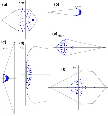
. Figure 3 provides several pictures of the sets
 $\mathcal Y_{c}$
, where the parameter c takes different values on the real line. In particular, Figures 3(a) and 3(f) correspond to the centers of the main cardioid and the hyperbolic component of period 2 respectively, and Figures 3(b) and 3(c) correspond to the parameter c lying slightly to the left and respectively slightly to the right of the cusp of the main cardioid. The blue dots are the values of
 $\nu _{\mathcal O}(c)$
, for all repelling periodic orbits
 $\mathcal O$
of periods up to and including eight. We do not know how accurate these pictures are, since inclusion of periodic orbits of higher periods can potentially change the convex hulls significantly.
Approximations of the sets
 $\mathcal Y_{c}$
as c changes along the real axis: (a)
 $c=0$
; (b)
 $c=0.24$
; (c)
 $c=0.26$
; (d)
 $c=0.42$
; (e)
 $c=-0.71$
; (f)
 $c=-1$
.