1 Introduction
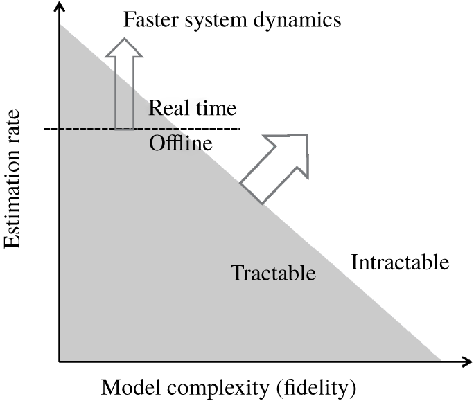
Reliably forecasting the state of a fluid system is crucial to diverse fields from meteorology to active flow control. Regardless of the application, flow estimation is constrained by available computational resources and the required estimation rate, i.e. the number of forecasts required per unit time. Figure 1 schematically explores the resulting trade off between model complexity ( $x$-axis) and estimation rate (
 $y$-axis). The grey area represents the set of problems for which the model complexity and estimation rate are achievable with available computational power. The horizontal dashed line represents the minimum estimation rate that would allow real-time prediction, as required for control. Many standard estimation techniques scale super-linearly with the number of degrees of freedom, which further limits model complexity for a fixed availability of computational power. Control engineers therefore favour low-rank models that preserve limited, but dynamically important, features of the system. Turbulence theorists, on the other hand, use all available computational power to simulate flows that are more complex (or accurate) than their predecessors, even if these simulations take months, there being no constraint beyond human endurance on the estimation rate.
In maximizing the estimation rate, a common approach is to use model reduction techniques such as balanced truncation (Ahuja & Rowley Reference Ahuja and Rowley2010) or eigenvalue realization algorithm (Flinois & Morgans Reference Flinois and Morgans2016) and retain only a few dynamically important modes. The resulting reduced-order models can be made small enough to allow the use of the standard algorithms, but their well-known fragility to the specification of initial conditions and flow parameters (e.g. Reynolds number) constitutes a major limitation in applications. It would therefore be desirable to seek more robust solutions that combine efficiency with a better representation of the physics. In figure 1, such solutions would lie close to the intersection of the real-time barrier (horizontal line) with the computational power barrier (boundary of grey region). As computational power increases (i.e. as the grey area expands), more complex models can be embedded in controllers, but in order to maximize the model complexity, estimation techniques that scale linearly (or as close to linearly as possible) with the number of degrees of freedom should be pursued.
Schematics of the current development of estimation techniques in the fluid mechanics context.

Researchers in meteorology and geophysics also sought estimation algorithms capable of handling high-dimensional models and large volumes of data, even if the estimation rate need not be particularly fast (Rabier Reference Rabier2005). Extending these techniques to engineering-scale flows is challenging due to the typically much faster time scale (and faster required estimation rate for control) over which they evolve. Colburn, Cessna & Bewley (Reference Colburn, Cessna and Bewley2011) applied an ensemble Kalman filter (EnKF) to the problem of estimating the statistics of the three-dimensional (3-D) turbulent channel flow. Kikuchi, Misaka & Obayashi (Reference Kikuchi, Misaka and Obayashi2015) compared the performance of a EnKF and a particle filter applied to a proper orthogonal decomposition (POD)-Galerkin model of the problem of the flow past a cylinder. Kato et al. (Reference Kato, Yoshizawa, Ueno and Obayashi2015) used a variation of the EnKF to achieve synchronization between a RANS-SA (Reynolds-averaged Navier–Stokes equations with Spalart–Allmaras turbulence model) numerical simulation of a steady transonic flow past airfoils and pressure experimental data. Mons et al. (Reference Mons, Chassaing, Gomez and Sagaut2016) used a Kalman smoother and other variational methods to reconstruct free-stream perturbation history based on measurements taken on and around a circular cylinder subjected to it. da Silva & Colonius (Reference da Silva and Colonius2018) used an EnKF-based estimator to estimate free-stream perturbations from pressure measurements taken on the surface of a NACA 0009 airfoil at high angle of attack. Darakananda et al. (Reference Darakananda, da Silva, Colonius and Eldredge2018) used the EnKF in conjunction with an aggregated vortex model to estimate the lift of an inclined flat plate subjected to gusts.
These efforts notwithstanding, the success of the estimator is contingent on the accuracy of the model chosen to represent the dynamics, and essentially any aspect of the chosen model that falls short of reality is a potential source of bias. Particular model errors include resolution (truncation error), turbulence models and uncertain initial and boundary conditions. Some of these involve a compromise between accuracy and cost to achieve a certain estimation rate with available computational power. Recently developed multi-fidelity (Houtekamer & Zhang Reference Houtekamer and Zhang2016) and multi-level (Hoel, Law & Tempone Reference Hoel, Law and Tempone2016) Monte Carlo approaches would allow for a more efficient use of the available resources, as they leverage information from a hierarchy of models with different fidelities (and costs) in order to minimize the overall cost of achieving a given estimation accuracy. Although promising, the integration of these techniques to the Kalman filtering framework is still work in progress with associated limitations. Hoel et al. (Reference Hoel, Law and Tempone2016), for instance, assumes that the ensemble size is the same for all resolution levels. Since we almost always use the minimum ensemble size that allows us to capture the most important degrees of freedom of the system, this approach will necessarily lead to a more expensive estimator than its single-level counterparts.
Friedland (Reference Friedland1969) was one of the first to propose a direct treatment of the model error. He proposed a two-stage sequential estimator, termed the separate-bias Kalman filter, in which model state and bias vector were treated independently. Dee & Da Silva (Reference Dee and Da Silva1998) provided a rigorous method to independently estimate and sequentially correct for forecast bias. Drecourt, Madsen & Rosbjerg (Reference Drecourt, Madsen and Rosbjerg2006) compared this method to the coloured-noise Kalman filter, in which the state vector is augmented to account for noise processes modelled by autoregressive models. Trémolet (Reference Trémolet2006) studied the introduction of bias models to a 3-D/4-D-Var framework, but assumed a full-rank time-invariant representation of the bias.
These works, however, all assume that the observation model, the function applied to the estimated system state to determine the observable to be compared to measurement, is unbiased. Many of the errors mentioned above can render both the dynamics and the observation models biased, with non-zero mean in any ensemble. Biased errors can be particularly harmful in the context of ensemble methods with an ensemble size much smaller than the number of degrees of freedom (which is the case for most of the practical applications). Even if the underlying dynamics is inherently low-dimensional, i.e. a few POD modes are responsible for most the system variance, discretization errors may have little support on those modes. Since the corrections applied to forecast state lie in the low-dimensional subspace spanned by the prior ensemble perturbations, large dynamic bias renders the true state of the system unreachable.
The observation model is also subject to discretization errors and the other sources of bias mentioned above. The error is essentially one of aliasing: even if the correct flow state is sampled the discretized observation model can be in error, especially when the observable is a nonlinear function of the state.
An additional source of error in the observation model is related to the optimality of the filtering scheme when nonlinear observation functions are present. When it was first introduced (Evensen Reference Evensen1994), the EnKF analysis scheme was initially derived for strictly linear observation functions, and extensions inspired by the extended Kalman filter and the iterated Kalman filter (Jazwinski Reference Jazwinski1970) were later proposed to allow for measurements that relate to the state through a nonlinear map (Zupanski Reference Zupanski2005; Gu & Oliver Reference Gu and Oliver2007). Even though the EnKF forecast step is intrinsically capable (at least partially) of dealing with nonlinear dynamical models due to its Monte Carlo-like strategy, the analysis step itself may be rendered biased (or suboptimal) if nonlinearities cause the posterior distribution to no longer be Gaussian (Jazwinski Reference Jazwinski1970).
In this work, a direct treatment of the discretization bias of both forecast and observation models is proposed aiming to equip the standard EnKF framework to deal with imperfect models. In § 2, we demonstrate that low-resolution models give rise to biased estimates. In § 2.1, these errors are modelled as low rank by representing the relevant features of the bias as coloured-noise processes. After briefly describing the standard EnKF scheme in § 3, the proposed bias-aware methodology is summarized in § 4. Section 5 describes the numerical experiments used to assess the performance and § 6 lists some of the main conclusions of this work and proposes future research directions.
2 Discretization error as a source of bias
Let  $\tilde{f}(\boldsymbol{x})$ be the exact transition function of the Navier–Stokes equations, which maps the infinite-dimensional solution
 $\tilde{\boldsymbol{x}}_{k-1}$ at time
 $t_{k-1}$ to the solution
 $\tilde{\boldsymbol{x}}_{k}$ at time
 $t_{k}$, and let
 $\tilde{h}$ represent a (potentially nonlinear) function that maps the exact flow state to a
 $p$-dimensional vector of observables,
 $\boldsymbol{y}_{k}$,
 $$\begin{eqnarray}\displaystyle & \displaystyle \tilde{\boldsymbol{x}}_{k}=\tilde{f}(\tilde{\boldsymbol{x}}_{k-1}), & \displaystyle\end{eqnarray}$$
 $$\begin{eqnarray}\displaystyle & \displaystyle \boldsymbol{y}_{k}=\tilde{h}(\tilde{\boldsymbol{x}}_{k})+\unicode[STIX]{x1D750}_{k}^{m}, & \displaystyle\end{eqnarray}$$
 $\unicode[STIX]{x1D750}_{k}^{m}\sim N(0,\tilde{R}_{k})$ is a
 $p$-dimensional random error vector associated with the measurement methodology that is independent of the state and uncorrelated in time.
Since both the state  $\tilde{\boldsymbol{x}}$ and the operators
 $\tilde{f}$ and
 $\tilde{h}$ are unattainable for practical purposes, we introduce a finite-dimensional approximation for the model and state. We notate their finite
 $n$-dimensional approximations with the same symbols but without the tilde. Following Cohn (Reference Cohn1997), we define a projection operator
 $\unicode[STIX]{x1D6F1}$ that maps the true state
 $\tilde{\boldsymbol{x}}_{k}$ onto its finite-dimensional representation
 $\boldsymbol{x}_{k}=\unicode[STIX]{x1D6F1}\tilde{\boldsymbol{x}}_{k}$. The propagation of
 $\boldsymbol{x}_{k}$ can be represented as
 $$\begin{eqnarray}\boldsymbol{x}_{k}=f(\boldsymbol{x}_{k-1})+\unicode[STIX]{x1D739}_{k},\end{eqnarray}$$
where
 $$\begin{eqnarray}\displaystyle \unicode[STIX]{x1D739}_{k}=\unicode[STIX]{x1D6F1}\tilde{f}(\tilde{\boldsymbol{x}}_{k-1})-f(\unicode[STIX]{x1D6F1}\tilde{\boldsymbol{x}}_{k-1}). & & \displaystyle\end{eqnarray}$$
The forcing term  $\unicode[STIX]{x1D739}_{k}$ represents the model error, and gathers errors from different sources: discretization error, inaccurate boundary conditions, uncertain forcing and so on. Analogously, since the continuous state is never available for practical purposes, a discrete version of the observation operator
 $h(\cdot )$ needs to be introduced
 $$\begin{eqnarray}\boldsymbol{y}_{k}=h_{k}(\boldsymbol{x}_{k})+\unicode[STIX]{x1D750}_{k}^{m}+\unicode[STIX]{x1D750}_{k}^{r},\end{eqnarray}$$
where
 $$\begin{eqnarray}\displaystyle \unicode[STIX]{x1D750}_{k}^{r} & = & \displaystyle \tilde{h}(\tilde{\boldsymbol{x}}_{k})-h(\unicode[STIX]{x1D6F1}\tilde{\boldsymbol{x}}_{k})\nonumber\\ \displaystyle & = & \displaystyle (\tilde{h}(\tilde{\boldsymbol{x}}_{k})-\tilde{h}(\unicode[STIX]{x1D6F1}\tilde{\boldsymbol{x}}_{k}))+(\tilde{h}(\unicode[STIX]{x1D6F1}\tilde{\boldsymbol{x}}_{k})-h(\unicode[STIX]{x1D6F1}\tilde{\boldsymbol{x}}_{k}))\end{eqnarray}$$
is the error of representativeness (Cohn Reference Cohn1997), which can be viewed as either a discretization error or a modelling error due to the complexity of the mapping between the control space and the observation space. This error can be further split into two contributions: a first term that represents the effect of the exact operator on the unresolved scales (aliasing), and a second term that represents the discretization error of the operator itself.
Because  $\unicode[STIX]{x1D739}_{k}$ depends not only on the state but also on the continuous operator
 $\tilde{f}$, its value is unknowable from a practical point of view. Therefore, the most common approach is to represent this error as a stochastic process with known bias and covariance. A stochastic process is an indexed family of random variables that is commonly used to represent the time evolution of a random phenomenon. Still, a complete representation of
 $\unicode[STIX]{x1D739}_{k}$ requires estimation of all
 $n(n+1)/2$ degrees of freedom of the associated covariance matrix, which is impractical regardless of the estimation procedure used (Dee Reference Dee1995). In the next section, we propose a low-rank model for it, as well as for the associated measurement resolution error,
 $\unicode[STIX]{x1D750}_{k}^{r}$.
2.1 Low-rank representation of the bias
We propose a model for the error
 $$\begin{eqnarray}\unicode[STIX]{x1D739}_{k}=\unicode[STIX]{x1D71E}_{x}\unicode[STIX]{x1D743}_{k}+\unicode[STIX]{x1D741}_{k},\end{eqnarray}$$
where the first term comprises the non-zero-mean bias error that represents the available deterministic knowledge about the error, and the second term represents a zero-mean random error. Within the first term,  $\unicode[STIX]{x1D71E}_{x}\in \mathbb{R}^{n\times n_{s}}$ is a low-rank representation of the spatial distribution of the error, determined a priori from available data, and
 $\unicode[STIX]{x1D743}_{k}$ are time-varying, time-correlated coefficients that will be estimated online. We anticipate that the first term will represent the slowly varying time-correlated dynamics of the error whereas the second term will represent the fast-varying time-uncorrelated dynamics, which we model as white noise (
 $\unicode[STIX]{x1D741}_{k}\sim N(0,\unicode[STIX]{x1D64C}_{k})$, i.e.
 $\unicode[STIX]{x1D741}_{k}$ is a random vector that has a normal distribution with zero mean and covariance matrix
 $\unicode[STIX]{x1D64C}_{k}$). In meteorology, Dee (Reference Dee1995) and Cohn & Parrish (Reference Cohn and Parrish1991) have proposed representing
 $\unicode[STIX]{x1D739}_{k}$ as a single random variable
 $\unicode[STIX]{x1D741}_{k}$ whose covariance matrix
 $\unicode[STIX]{x1D64C}_{k}$ had parameters that could be tuned online. It is interesting to note that these models often rely on using the slow modes of the forecast model to achieve a low-order representation of the random part of the bias. This approach correctly recognizes the slowly varying behaviour and the low-dimensionality of the bias, but fails to represent its time correlation and non-zero mean.
The measurement resolution error can be split in two analogous terms
 $$\begin{eqnarray}\unicode[STIX]{x1D750}_{k}^{r}=\unicode[STIX]{x1D71E}_{y}\boldsymbol{\unicode[STIX]{x1D702}}_{k}+\unicode[STIX]{x1D742}_{k},\end{eqnarray}$$
where  $\unicode[STIX]{x1D71E}_{y}\in \mathbb{R}^{p\times n_{o}}$ is a low-rank modal representation of the bias, and
 $\unicode[STIX]{x1D742}_{k}\sim N(0,\unicode[STIX]{x1D64D}^{r})$ represents random errors in the measurement function, modelled as a zero-mean Gaussian process. The latter can be merged with the measurement accuracy error
 $\unicode[STIX]{x1D750}_{k}^{m}$ in (2.4), which in sum is represented as a zero-mean Gaussian process with a combined covariance matrix
 $\unicode[STIX]{x1D64D}$.
As will be discussed in § 5.2, suitable representations for  $\unicode[STIX]{x1D71E}_{x}$ and
 $\unicode[STIX]{x1D71E}_{y}$ can be obtained using data processing tools such as POD (Holmes et al. Reference Holmes, Lumley, Berkooz and Rowley2012) to obtain the spatial modes that best represent the expected variance of the bias. Note that, in this formulation, all temporal information is contained in the bias parameters
 $\unicode[STIX]{x1D743}\in \mathbb{R}^{n_{s}}$ and
 $\boldsymbol{\unicode[STIX]{x1D702}}\in \mathbb{R}^{n_{o}}$.
We expect that  $\unicode[STIX]{x1D743}_{k}$ and
 $\boldsymbol{\unicode[STIX]{x1D702}}_{k}$ are auto-correlated (and maybe cross-correlated) in time. As a first option, autoregressive models (AR) are the simplest way of representing this feature in the discrete-time framework. AR models differ from moving-average models by the fact that, in the former, the weights are applied to the previous states, while, in the latter, the weights are applied to the input (noise). Noise sequences obeying AR models are often referred to as coloured-noise sequences (Drecourt et al. Reference Drecourt, Madsen and Rosbjerg2006; Chui & Chen Reference Chui and Chen2009). If
 $N_{x}$ and
 $N_{y}$ are the orders for the autoregressive models for the state and observation bias, respectively, then
 $$\begin{eqnarray}\displaystyle & \displaystyle \unicode[STIX]{x1D743}_{k}=\bar{\unicode[STIX]{x1D743}}+\mathop{\sum }_{i=1}^{N_{x}}\unicode[STIX]{x1D6F7}_{i}^{x}(\unicode[STIX]{x1D743}_{k-i}-\bar{\unicode[STIX]{x1D743}})+\unicode[STIX]{x1D738}_{x,k}, & \displaystyle\end{eqnarray}$$
 $$\begin{eqnarray}\displaystyle & \displaystyle \boldsymbol{\unicode[STIX]{x1D702}}_{k}=\bar{\boldsymbol{\unicode[STIX]{x1D702}}}+\mathop{\sum }_{i=1}^{N_{y}}\unicode[STIX]{x1D6F7}_{i}^{y}(\boldsymbol{\unicode[STIX]{x1D702}}_{k-i}-\bar{\boldsymbol{\unicode[STIX]{x1D702}}})+\unicode[STIX]{x1D738}_{y,k}, & \displaystyle\end{eqnarray}$$
where  $\unicode[STIX]{x1D738}_{x,k}\sim N(0,\unicode[STIX]{x1D64C}^{b})$ and
 $\unicode[STIX]{x1D738}_{y,k}\sim N(0,\unicode[STIX]{x1D64D}^{b})$, and
 $\unicode[STIX]{x1D6F7}_{i}^{x}$ and
 $\unicode[STIX]{x1D6F7}_{i}^{y}$ should be determined based on prior knowledge about the system under study. Both
 $\unicode[STIX]{x1D743}$ and
 $\boldsymbol{\unicode[STIX]{x1D702}}$ are assumed to only depend on time, and the bar denotes time-averaged variables. For example, if the Markov condition holds (
 $N_{x}=N_{y}=1$) and these error terms are supposed to vary on a much slower time scale than the state dynamics, one can choose to use a persistent model and set
 $\unicode[STIX]{x1D6F7}^{x}=\unicode[STIX]{x1D6F7}^{y}=1$.
A second possibility that can be more suitable for periodic flows is to represent the bias as a sum of harmonics of the system’s characteristic frequency. In this framework, the columns of  $\unicode[STIX]{x1D71E}_{x}$ and
 $\unicode[STIX]{x1D71E}_{y}$ and the bias coefficients
 $\unicode[STIX]{x1D743}_{k}$ and
 $\boldsymbol{\unicode[STIX]{x1D702}}_{k}$ are represented by complex vectors, and the bias dynamics is then given by
 $$\begin{eqnarray}\displaystyle & \displaystyle \unicode[STIX]{x1D739}_{k}=\text{Re}(\unicode[STIX]{x1D71E}_{x}\unicode[STIX]{x1D743}_{k})+\unicode[STIX]{x1D741}_{k}, & \displaystyle\end{eqnarray}$$
 $$\begin{eqnarray}\displaystyle & \displaystyle \unicode[STIX]{x1D750}_{k}^{r}=\text{Re}(\unicode[STIX]{x1D71E}_{y}\boldsymbol{\unicode[STIX]{x1D702}}_{k})+\unicode[STIX]{x1D742}_{k}, & \displaystyle\end{eqnarray}$$
and
 $$\begin{eqnarray}\displaystyle & \displaystyle \unicode[STIX]{x1D743}_{k}=\exp (\unicode[STIX]{x1D726}_{x}\unicode[STIX]{x0394}t)\unicode[STIX]{x1D743}_{k-1}+\unicode[STIX]{x1D738}_{x,k}, & \displaystyle\end{eqnarray}$$
 $$\begin{eqnarray}\displaystyle & \displaystyle \boldsymbol{\unicode[STIX]{x1D702}}_{k}=\exp (\unicode[STIX]{x1D726}_{y}\unicode[STIX]{x0394}t)\boldsymbol{\unicode[STIX]{x1D702}}_{k-1}+\unicode[STIX]{x1D738}_{y,k}, & \displaystyle\end{eqnarray}$$
where  $\unicode[STIX]{x1D726}_{x}$ and
 $\unicode[STIX]{x1D726}_{y}$ are diagonal matrices whose entries are also complex numbers. The real part of these entries represents the mode’s growth/decay rate, which is expected to be zero in a purely periodic flow, and the corresponding imaginary part is related to the mode’s oscillatory frequency. Note that the noise terms
 $\unicode[STIX]{x1D738}_{x}$ and
 $\unicode[STIX]{x1D738}_{y}$ are now complex random sequences with zero-mean Gaussian-distributed magnitude, but uniformly distributed phase. Data processing tools such as the dynamic mode decomposition (DMD), proposed by Schmid (Reference Schmid2010), can be used to determine suitable matrices
 $\unicode[STIX]{x1D71E}$ and
 $\unicode[STIX]{x1D726}$ in this case, as will be discussed in § 5.2.
In order to take advantage of an eventual non-zero cross-correlation between the bias parameters  $\unicode[STIX]{x1D743}$ and
 $\boldsymbol{\unicode[STIX]{x1D702}}$ and the state
 $\boldsymbol{x}$ in the filtering process, these variables are gathered in an augmented state vector (
 $\boldsymbol{z}=[\boldsymbol{x}^{T}\unicode[STIX]{x1D743}^{T}\boldsymbol{\unicode[STIX]{x1D702}}^{T}]^{T}$) that will be estimated using the algorithm proposed in § 4.
3 The standard EnKF
Aiming at overcoming the computational cost limitation associated with the use of standard techniques such as the classical Kalman filter (KF) or its nonlinear generalizations for high-dimensional systems (for instance, the extended Kalman filter (EKF) (Gelb Reference Gelb1974) or the unscented Kalman filter (Julier & Uhlmann Reference Julier and Uhlmann2004)), Evensen (Reference Evensen1994) proposed a Monte Carlo approximation to the KF, termed the EnKF. According to this methodology, the internal state of the estimator is represented by an ensemble of particles whose statistics of interest, namely its ensemble mean ( $\bar{\boldsymbol{x}}$) and covariance matrix (
 $\hat{\unicode[STIX]{x1D63E}}$), are used to approximate their population counterpart.
Since then, this method has been extensively used for high-dimensional systems (thousands of degrees of freedom or more) associated with a computationally onerous forecast (as in meteorology, oceanography and geophysical flows, e.g. Houtekamer & Zhang (Reference Houtekamer and Zhang2016), Bengtsson, Snyder & Nychka (Reference Bengtsson, Snyder and Nychka2003), Evensen (Reference Evensen2004) and Anderson & Anderson (Reference Anderson and Anderson1999)). In such contexts, this technique has shown to provide an accurate estimate of the first two moments of the state of the system even for a small ensemble size (provided that the Gaussian assumption appears to hold, see Papadakis et al. (Reference Papadakis, Mémin, Cuzol and Gengembre2010)).
Apart from the more favourable scaleup with the number of degrees of freedom (and associated reduction in memory requirements), other advantages of the EnKF in comparison to the variational methods or standard KF formulations are that it does not require the adjoint of the dynamical model, it has a natural probabilistic interpretation under a Bayesian perspective and, due to its formulation in terms of independent particles, it is embarrassingly parallel.
3.1 Notation
Consider representing the state  $\boldsymbol{x}\in \mathbb{R}^{n}$ of the system as an ensemble of
 $q$ initially independent states sampled from a normal distribution with predefined mean and covariance matrix. The expected value of the state corresponds to the ensemble average of these particles
 $$\begin{eqnarray}\bar{\boldsymbol{x}}_{k}=\frac{1}{q}\mathop{\sum }_{j=1}^{q}\boldsymbol{x}_{k}^{(j)},\end{eqnarray}$$
where the subscript  $k$ refers to the time index and the superscript
 $(j)$ refers to the ensemble member index.
Defining the scaled state perturbation matrix  $\unicode[STIX]{x1D63C}_{k}\in \mathbb{R}^{n\times q}$ as
 $$\begin{eqnarray}\unicode[STIX]{x1D63C}_{k}=\frac{1}{\sqrt{q-1}}[\boldsymbol{x}_{k}^{(1)}-\bar{\boldsymbol{x}}_{k}\cdots \boldsymbol{x}_{k}^{(q)}-\bar{\boldsymbol{x}}_{k}],\end{eqnarray}$$
one can finally compute the ensemble covariance matrix
 $$\begin{eqnarray}\unicode[STIX]{x1D63E}_{k}=\unicode[STIX]{x1D63C}_{k}(\unicode[STIX]{x1D63C}_{k})^{T},\end{eqnarray}$$
which is an estimate of the state covariance matrix.
Similarly, the scaled output perturbation matrix  $\unicode[STIX]{x1D643}\unicode[STIX]{x1D63C}_{k}\in \mathbb{R}^{p\times q}$ (assuming the linearity of the observation function, i.e.
 $h(\boldsymbol{x})=\unicode[STIX]{x1D643}\boldsymbol{x}$) can be defined as
 $$\begin{eqnarray}\unicode[STIX]{x1D643}\unicode[STIX]{x1D63C}_{k}=\frac{1}{\sqrt{q-1}}[\boldsymbol{y}_{k}^{(1)}-\bar{\boldsymbol{y}}_{k}\cdots \boldsymbol{y}_{k}^{(q)}-\bar{\boldsymbol{y}}_{k}],\end{eqnarray}$$
where  $\boldsymbol{y}_{k}^{(j)}=h(\boldsymbol{x}_{k}^{(j)})$ and
 $\bar{\boldsymbol{y}}_{k}$ is the ensemble average of the outputs.
3.2 Algorithm
The filtering algorithm can be summarized as a succession of two steps, a forecast step (or dynamic update) and a analysis step (or measurement update), that are performed sequentially as time moves on. Algorithm 1 in appendix A shows an overview of these steps, which are described below.
3.2.1 Forecast step
The state of each ensemble member (here denoted by the superscript  $(j)$) at the next time step is estimated using the (possibly nonlinear) dynamic model
 $$\begin{eqnarray}\hat{\boldsymbol{x}}_{k+1}^{(j)}=f(\boldsymbol{x}_{k}^{(j)},\boldsymbol{u}_{k})+\unicode[STIX]{x1D741}_{k}^{(j)},\end{eqnarray}$$
where the hat is used to represent forecast state variables,  $\boldsymbol{u}_{k}$ is some control variable and
 $\unicode[STIX]{x1D741}_{k}^{(j)}$ is a realization of the process noise (here assumed to have zero mean). If applied to a efficient implementation of the dynamics (with complexity
 $O(n)$, for instance), this ensemble approach reduces the cost associated with the time propagation of the state statistics from
 $O(n^{2})$ (classical KF) to
 $O(nq)$ (EnKF). Since typical ensemble sizes are no larger than
 $O(10^{2})$, the overall cost is usually reduced by several orders of magnitude.
3.2.2 Analysis step
Bayes’ theorem can be used to combine the probability density function (PDF) of the forecast state (often referred to as the prior distribution) with newly available measurement statistics to produce the PDF of the analysed state (often referred to as the posterior distribution). The formal solution to the Kalman filtering problem is defined as the state that minimizes the conditional expectation of the mean-square error, i.e. the mean of the posterior distribution (Jazwinski Reference Jazwinski1970).
There are different ways of interpreting this definition, including as an optimization problem. Following this approach, the ensemble members are corrected in order to minimize the error with respect to the measurements in the presence of noise and model uncertainties. In other words, we look for the minimizer of the cost function (Law, Stuart & Zygalakis Reference Law, Stuart and Zygalakis2015)
 $$\begin{eqnarray}J(\boldsymbol{x})=\frac{1}{2\unicode[STIX]{x1D6FC}}\Vert \boldsymbol{x}-\hat{\boldsymbol{x}}_{k}^{(j)}\Vert _{\hat{\unicode[STIX]{x1D63E}}_{k}}^{2}+\frac{1}{2}\Vert \boldsymbol{y}_{k}-\unicode[STIX]{x1D643}\boldsymbol{x}\Vert _{\unicode[STIX]{x1D64D}}^{2},\end{eqnarray}$$
where  $\unicode[STIX]{x1D6FC}$ is a covariance inflation (CI) parameter (further details on CI schemes can be found in appendix B).
The first term in the cost function acts as a regularization term by penalizing the distance of the state to the prior estimate, and the second term penalizes the data mismatch between the observed measurement  $\boldsymbol{y}_{k}$ and that predicted by the observation model. The relative reliability of these two models is prescribed by the matrices
 $\unicode[STIX]{x1D64D}$ (measurement noise covariance matrix) and
 $\hat{\unicode[STIX]{x1D63E}}_{k}$ (prior ensemble state covariance). If, for example, the observation function is linear, the posterior is guaranteed to remain Gaussian and, the maximum-likelihood estimate (posterior mode) is also the minimum-variance estimate (posterior mean).
The solution corresponding to the minimum of (3.6) is given by
 $$\begin{eqnarray}\displaystyle \boldsymbol{x}_{k}^{(j)} & = & \displaystyle \hat{\boldsymbol{x}}_{k}^{(j)}+\unicode[STIX]{x1D6FC}\hat{\unicode[STIX]{x1D63C}}[\unicode[STIX]{x1D644}+\unicode[STIX]{x1D6FC}(\unicode[STIX]{x1D643}\hat{\unicode[STIX]{x1D63C}}_{k})^{T}\unicode[STIX]{x1D64D}^{-1}(\unicode[STIX]{x1D643}\hat{\unicode[STIX]{x1D63C}}_{k})]^{-1}(\unicode[STIX]{x1D643}\hat{\unicode[STIX]{x1D63C}}_{k})^{T}\unicode[STIX]{x1D64D}^{-1}(\boldsymbol{y}_{k}-\unicode[STIX]{x1D643}\hat{\boldsymbol{x}}_{k}^{(j)})\end{eqnarray}$$
 $$\begin{eqnarray}\displaystyle & = & \displaystyle \hat{\boldsymbol{x}}_{k}^{(j)}+\unicode[STIX]{x1D6FC}\hat{\unicode[STIX]{x1D63C}}_{k}(\unicode[STIX]{x1D643}\hat{\unicode[STIX]{x1D63C}}_{k})^{T}[\unicode[STIX]{x1D64D}+\unicode[STIX]{x1D6FC}(\unicode[STIX]{x1D643}\hat{\unicode[STIX]{x1D63C}}_{k})(\unicode[STIX]{x1D643}\hat{\unicode[STIX]{x1D63C}}_{k})^{T}]^{-1}(\boldsymbol{y}_{k}-\unicode[STIX]{x1D643}\hat{\boldsymbol{x}}_{k}^{(j)}),\end{eqnarray}$$
Notice that, here, we have the possibility of choosing between performing the analysis in the ensemble space ( $q$-by-
 $q$ matrix inversion – equation (3.7a)), or in the measurement space (
 $p$-by-
 $p$ matrix inversion – equation (3.7b)), depending on which one is more advantageous (Sakov, Evensen & Bertino Reference Sakov, Evensen and Bertino2009; Law et al. Reference Law, Stuart and Zygalakis2015). In either case, provided that
 $q\ll n$ or
 $p\ll n$, there is a significant reduction in computational expense when compared to the KF/EKF.
Algorithmically, when the inversion is done in the measurement space, the representer formulation, proposed by Evensen & van Leeuwen (Reference Evensen and van Leeuwen1996), is used
 $$\begin{eqnarray}\displaystyle & \displaystyle [\unicode[STIX]{x1D64D}+\unicode[STIX]{x1D6FC}(\unicode[STIX]{x1D643}\hat{\unicode[STIX]{x1D63C}}_{k})(\unicode[STIX]{x1D643}\hat{\unicode[STIX]{x1D63C}}_{k})^{T}]\boldsymbol{b}_{k}=(\boldsymbol{y}_{k}-\unicode[STIX]{x1D643}\hat{\boldsymbol{x}}_{k}^{(j)}), & \displaystyle\end{eqnarray}$$
 $$\begin{eqnarray}\displaystyle & \displaystyle \boldsymbol{x}_{k}^{(j)}=\hat{\boldsymbol{x}}_{k}^{(j)}+\unicode[STIX]{x1D6FC}\hat{\unicode[STIX]{x1D63C}}_{k}(\unicode[STIX]{x1D643}\hat{\unicode[STIX]{x1D63C}}_{k})^{T}\boldsymbol{b}_{k}, & \displaystyle\end{eqnarray}$$
 $\hat{\unicode[STIX]{x1D63C}}_{k}(\unicode[STIX]{x1D643}\hat{\unicode[STIX]{x1D63C}}_{k})^{T}$ are called the representers and represent the influence vectors for each measurement. The vector
 $\boldsymbol{b}_{k}$ then represents the magnitude by which each of the representers actuates in
 $\hat{\boldsymbol{x}}$. Note that one never needs to explicitly compute the covariance
 $\hat{\unicode[STIX]{x1D63E}}_{k}$, since it suffices to evaluate
 $\hat{\unicode[STIX]{x1D63C}}_{k}(\unicode[STIX]{x1D643}\hat{\unicode[STIX]{x1D63C}}_{k})^{T}$ and
 $\unicode[STIX]{x1D643}\hat{\unicode[STIX]{x1D63C}}_{k}(\unicode[STIX]{x1D643}\hat{\unicode[STIX]{x1D63C}}_{k})^{T}$.
For each ensemble member,  $\boldsymbol{y}_{k}$ must be independently sampled from a normal distribution whose mean is the measurement vector obtained from the estimated system, and whose variance is
 $\unicode[STIX]{x1D64D}$. Due to this sampling step, this algorithm is often referred to as perturbed observations (or stochastic) EnKF. Although this procedure introduces an additional sampling error, Burgers, Jan van Leeuwen & Evensen (Reference Burgers, Jan van Leeuwen and Evensen1998) showed that the assumption of measurements being random variables is necessary to ensure an unbiased estimation of the evolution of the ensemble mean and covariance, provided that the ensemble size is large enough. Also, previous work by Lawson & Hansen (Reference Lawson and Hansen2004) suggested it performs better in the presence of nonlinearities than deterministic alternatives.
4 A bias-aware EnKF
Bias awareness can be achieved using the augmentation approach: the parameters corresponding to the low-rank bias models developed in the previous section are appended to the original state vector. The two filtering steps introduced in § 3 become:
Forecast step: The state of each ensemble member at the next time step is forecast using the (possibly nonlinear) dynamic model
 $$\begin{eqnarray}\displaystyle \hat{\boldsymbol{z}}_{k}^{(j)} & = & \displaystyle \left[\begin{array}{@{}c@{}}\hat{\boldsymbol{x}}_{k}^{(j)}\\ \hat{\unicode[STIX]{x1D743}}_{k}^{(j)}\\ \hat{\boldsymbol{\unicode[STIX]{x1D702}}}_{k}^{(j)}\end{array}\right]=f^{\dagger }(\boldsymbol{z}_{k-1}^{(j)})+\unicode[STIX]{x1D741}_{k}^{\dagger (j)}\nonumber\\ \displaystyle & = & \displaystyle \left[\begin{array}{@{}c@{}}f(\boldsymbol{x}_{k-1}^{(j)})\\ \bar{\unicode[STIX]{x1D743}}+\unicode[STIX]{x1D6F7}_{x}(\unicode[STIX]{x1D743}_{k-1}^{(j)}-\bar{\unicode[STIX]{x1D743}})\\ \bar{\boldsymbol{\unicode[STIX]{x1D702}}}+\unicode[STIX]{x1D6F7}_{y}(\boldsymbol{\unicode[STIX]{x1D702}}_{k-1}^{(j)}-\bar{\boldsymbol{\unicode[STIX]{x1D702}}})\end{array}\right]+\left[\begin{array}{@{}c@{}}\unicode[STIX]{x1D741}_{k}^{(j)}\\ \unicode[STIX]{x1D738}_{x,k}^{(j)}\\ \unicode[STIX]{x1D738}_{y,k}^{(j)}\end{array}\right],\end{eqnarray}$$
where all variables were previously defined in § 2. Assuming  $n_{s}\ll n$ and
 $n_{o}\ll n$, the additional cost associated with the bias dynamics should be negligible.
The prior statistics are defined as
 $$\begin{eqnarray}\displaystyle & \displaystyle \hat{\unicode[STIX]{x1D655}}_{k}=\left[\begin{array}{@{}cccc@{}}\hat{\boldsymbol{z}}_{k}^{(1)} & \hat{\boldsymbol{z}}_{k}^{(2)} & \cdots \, & \hat{\boldsymbol{z}}_{k}^{(q)}\end{array}\right], & \displaystyle\end{eqnarray}$$
 $$\begin{eqnarray}\displaystyle & \displaystyle \bar{\boldsymbol{z}}_{k}=\frac{1}{q}\hat{\unicode[STIX]{x1D655}}_{k}\unicode[STIX]{x1D7D9}, & \displaystyle\end{eqnarray}$$
 $$\begin{eqnarray}\displaystyle & \displaystyle \hat{\unicode[STIX]{x1D63E}}_{k}^{zz}=\frac{1}{\sqrt{q-1}}\mathop{\sum }_{i=1}^{q}(\hat{\boldsymbol{z}}_{k}^{(i)}-\bar{\boldsymbol{z}}_{k})(\hat{\boldsymbol{z}}_{k}^{(i)}-\bar{\boldsymbol{z}}_{k})^{T}, & \displaystyle\end{eqnarray}$$
 $\unicode[STIX]{x1D7D9}$ represents an
 $n$-dimensional vector with unitary entries. The ensemble covariance matrix can also be expressed in terms of the scaled ensemble perturbation matrix
 $$\begin{eqnarray}\displaystyle & \displaystyle \hat{\unicode[STIX]{x1D63C}}_{k}=\frac{1}{\sqrt{q-1}}\hat{\unicode[STIX]{x1D655}}_{k}(\unicode[STIX]{x1D644}-\bar{\boldsymbol{z}}_{k}\unicode[STIX]{x1D7D9}^{T}), & \displaystyle\end{eqnarray}$$
 $$\begin{eqnarray}\displaystyle & \displaystyle \hat{\unicode[STIX]{x1D63E}}_{k}^{zz}=\hat{\unicode[STIX]{x1D63C}}^{(j)}(\hat{\unicode[STIX]{x1D63C}}^{(j)})^{T}. & \displaystyle\end{eqnarray}$$
Analysis step: The optimization framework is used again to obtain the new analysis equations. For each of the ensemble members, provided that both the prior and the measurement distributions are Gaussian, the mode (maximum-likelihood estimate) of the posterior distribution corresponds to the minimizer of the cost function
 $$\begin{eqnarray}J(\boldsymbol{z})=\frac{1}{2\unicode[STIX]{x1D6FC}}\Vert \unicode[STIX]{x1D642}^{-1}\boldsymbol{z}-\hat{\boldsymbol{z}}_{k}^{(j)}\Vert _{\hat{\unicode[STIX]{x1D63E}}_{k}^{zz}}^{2}+\frac{1}{2}\Vert \boldsymbol{y}_{k}-h(\boldsymbol{x})-\unicode[STIX]{x1D71E}_{y}\boldsymbol{\unicode[STIX]{x1D702}}-\unicode[STIX]{x1D742}_{k}^{(j)}\Vert _{\unicode[STIX]{x1D64D}}^{2},\end{eqnarray}$$
while restricting  $[(\boldsymbol{x}-\unicode[STIX]{x1D71E}_{x}\unicode[STIX]{x1D743})^{T}\quad \unicode[STIX]{x1D743}^{T}\quad \boldsymbol{\unicode[STIX]{x1D702}}^{T}]^{T}=\unicode[STIX]{x1D642}^{-1}\boldsymbol{z}$ to the affine subset generated by the prior estimate of the state
 $\hat{\boldsymbol{z}}_{k}^{(j)}$ and the subspace spanned by the scaled perturbation matrix
 $\hat{\unicode[STIX]{x1D63C}}_{k}$, i.e.
 $$\begin{eqnarray}\boldsymbol{z}_{k}=\underset{\boldsymbol{z}\in \unicode[STIX]{x1D642}(\hat{\boldsymbol{z}}+\hat{\unicode[STIX]{x1D63C}}_{k})}{\text{argmin}}J(\boldsymbol{z}),\end{eqnarray}$$
where
 $$\begin{eqnarray}\unicode[STIX]{x1D642}=\left[\begin{array}{@{}ccc@{}}\unicode[STIX]{x1D644} & \unicode[STIX]{x1D71E}_{x} & \mathbf{0}\\ \mathbf{0} & \unicode[STIX]{x1D644} & \mathbf{0}\\ \mathbf{0} & \mathbf{0} & \unicode[STIX]{x1D644}\end{array}\right].\end{eqnarray}$$
4.1 The linear observation function case
When the observation function is linear, i.e.  $h(\boldsymbol{x})=\unicode[STIX]{x1D643}\boldsymbol{x}$, the observation equation can be written as
 $$\begin{eqnarray}\hat{\boldsymbol{y}}_{k}^{(j)}=\tilde{\unicode[STIX]{x1D643}}\unicode[STIX]{x1D642}\,\hat{\boldsymbol{z}}_{k}^{(j)}+\unicode[STIX]{x1D742}_{k}^{(j)},\end{eqnarray}$$
where
 $$\begin{eqnarray}\tilde{\unicode[STIX]{x1D643}}=\left[\begin{array}{@{}ccc@{}}\unicode[STIX]{x1D643} & \mathbf{0} & \unicode[STIX]{x1D71E}_{y}\end{array}\right].\end{eqnarray}$$
The restriction on the optimization space is enforced by means of a change of variables
 $$\begin{eqnarray}\displaystyle \boldsymbol{z} & = & \displaystyle \unicode[STIX]{x1D642}(\hat{\boldsymbol{z}}_{k}^{(j)}+\sqrt{\unicode[STIX]{x1D6FC}}\hat{\unicode[STIX]{x1D63C}}_{k}\boldsymbol{v})\nonumber\\ \displaystyle & = & \displaystyle \unicode[STIX]{x1D642}\,\hat{\boldsymbol{z}}_{k}^{(j)}+\sqrt{\unicode[STIX]{x1D6FC}}\hat{\unicode[STIX]{x1D63D}}_{k}\boldsymbol{v},\end{eqnarray}$$
where  $\boldsymbol{v}\in \mathbb{R}^{q}$ is the correction coefficient vector and
 $\hat{\unicode[STIX]{x1D63D}}_{k}=\unicode[STIX]{x1D642}\hat{\unicode[STIX]{x1D63C}}_{k}$ is the bias-corrected ensemble perturbation matrix.
The analysis step objective is then defined as finding
 $$\begin{eqnarray}\boldsymbol{v}_{k}=\underset{\boldsymbol{v}\in \mathbb{R}^{q}}{\text{argmin}}~J(\boldsymbol{v}),\end{eqnarray}$$
where
 $$\begin{eqnarray}J(\boldsymbol{v})={\textstyle \frac{1}{2}}\Vert \boldsymbol{v}\Vert ^{2}+{\textstyle \frac{1}{2}}\Vert \boldsymbol{y}_{k}-\tilde{\unicode[STIX]{x1D643}}\unicode[STIX]{x1D642}(\hat{\boldsymbol{z}}_{k}^{(j)}+\sqrt{\unicode[STIX]{x1D6FC}}\hat{\unicode[STIX]{x1D63C}}_{k}\boldsymbol{v})-\unicode[STIX]{x1D742}_{k}^{(j)}\Vert _{\unicode[STIX]{x1D64D}}^{2}.\end{eqnarray}$$
Since  $J(\boldsymbol{v})$ is quadratic in
 $\boldsymbol{v}$, the solution is unique and corresponds to the root of
 $$\begin{eqnarray}\boldsymbol{D}\boldsymbol{J}(\boldsymbol{v})=\boldsymbol{v}-\sqrt{\unicode[STIX]{x1D6FC}}(\tilde{\unicode[STIX]{x1D643}}\hat{\unicode[STIX]{x1D63D}}_{k})^{T}\unicode[STIX]{x1D64D}^{-1}(\boldsymbol{y}_{k}-\tilde{\unicode[STIX]{x1D643}}\unicode[STIX]{x1D642}\,\hat{\boldsymbol{z}}_{k}^{(j)}-\sqrt{\unicode[STIX]{x1D6FC}}\tilde{\unicode[STIX]{x1D643}}\hat{\unicode[STIX]{x1D63D}}_{k}\boldsymbol{v}-\unicode[STIX]{x1D742}_{k}^{(j)})=0,\end{eqnarray}$$
which is given by
 $$\begin{eqnarray}\displaystyle \boldsymbol{v}_{k}^{(j)} & = & \displaystyle \sqrt{\unicode[STIX]{x1D6FC}}[\unicode[STIX]{x1D644}+\unicode[STIX]{x1D6FC}(\tilde{\unicode[STIX]{x1D643}}\hat{\unicode[STIX]{x1D63D}}_{k})^{T}\unicode[STIX]{x1D64D}^{-1}(\tilde{\unicode[STIX]{x1D643}}\hat{\unicode[STIX]{x1D63D}}_{k})]^{-1}(\tilde{\unicode[STIX]{x1D643}}\hat{\unicode[STIX]{x1D63D}}_{k})^{T}\unicode[STIX]{x1D64D}^{-1}(\boldsymbol{y}_{k}-\tilde{\unicode[STIX]{x1D643}}\unicode[STIX]{x1D642}\hat{\boldsymbol{z}}_{k}^{(j)}-\unicode[STIX]{x1D742}_{k}^{(j)}),\end{eqnarray}$$
 $$\begin{eqnarray}\displaystyle & = & \displaystyle \sqrt{\unicode[STIX]{x1D6FC}}(\tilde{\unicode[STIX]{x1D643}}\hat{\unicode[STIX]{x1D63D}}_{k})^{T}[\unicode[STIX]{x1D64D}+\unicode[STIX]{x1D6FC}(\tilde{\unicode[STIX]{x1D643}}\hat{\unicode[STIX]{x1D63D}}_{k})(\tilde{\unicode[STIX]{x1D643}}\hat{\unicode[STIX]{x1D63D}}_{k})^{T}]^{-1}(\boldsymbol{y}_{k}-\tilde{\unicode[STIX]{x1D643}}\unicode[STIX]{x1D642}\hat{\boldsymbol{z}}_{k}^{(j)}-\unicode[STIX]{x1D742}_{k}^{(j)}),\end{eqnarray}$$
 $q$-by-
 $q$ matrix – equation (4.13a)), or in the measurement space (solution of a
 $p$-by-
 $p$ matrix – equation (4.13b)), depending on which is smaller.
The final solution is then obtained by projecting these coefficients back to the state space
 $$\begin{eqnarray}\displaystyle \boldsymbol{z}_{k}^{(j)} & = & \displaystyle \unicode[STIX]{x1D642}\,\hat{\boldsymbol{z}}_{k}^{(j)}+\unicode[STIX]{x1D6FC}\hat{\unicode[STIX]{x1D63D}}_{k}[\unicode[STIX]{x1D644}+\unicode[STIX]{x1D6FC}(\tilde{\unicode[STIX]{x1D643}}\hat{\unicode[STIX]{x1D63D}}_{k})^{T}\unicode[STIX]{x1D64D}^{-1}(\tilde{\unicode[STIX]{x1D643}}\hat{\unicode[STIX]{x1D63D}}_{k})]^{-1}(\tilde{\unicode[STIX]{x1D643}}\hat{\unicode[STIX]{x1D63D}}_{k})^{T}\unicode[STIX]{x1D64D}^{-1}\nonumber\\ \displaystyle & & \displaystyle \times \,(\boldsymbol{y}_{k}-\tilde{\unicode[STIX]{x1D643}}\unicode[STIX]{x1D642}\,\hat{\boldsymbol{z}}_{k}^{(j)}-\unicode[STIX]{x1D742}_{k}^{(j)}),\end{eqnarray}$$
 $$\begin{eqnarray}\displaystyle & = & \displaystyle \unicode[STIX]{x1D642}\,\hat{\boldsymbol{z}}_{k}^{(j)}+\unicode[STIX]{x1D6FC}\hat{\unicode[STIX]{x1D63D}}_{k}(\tilde{\unicode[STIX]{x1D643}}\hat{\unicode[STIX]{x1D63D}}_{k})^{T}[\unicode[STIX]{x1D64D}+\unicode[STIX]{x1D6FC}(\tilde{\unicode[STIX]{x1D643}}\hat{\unicode[STIX]{x1D63D}}_{k})(\tilde{\unicode[STIX]{x1D643}}\hat{\unicode[STIX]{x1D63D}}_{k})^{T}]^{-1}\nonumber\\ \displaystyle & & \displaystyle \times \,(\boldsymbol{y}_{k}-\tilde{\unicode[STIX]{x1D643}}\unicode[STIX]{x1D642}\,\hat{\boldsymbol{z}}_{k}^{(j)}-\unicode[STIX]{x1D742}_{k}^{(j)}).\end{eqnarray}$$
Algorithmically, when the inversion is done in the measurement space, instead of solving for  $\boldsymbol{v}_{k}$, the representer formulation (Evensen & van Leeuwen Reference Evensen and van Leeuwen1996) is used
 $$\begin{eqnarray}\displaystyle & \displaystyle [\unicode[STIX]{x1D64D}+\unicode[STIX]{x1D6FC}(\tilde{\unicode[STIX]{x1D643}}\hat{\unicode[STIX]{x1D63D}}_{k})(\tilde{\unicode[STIX]{x1D643}}\hat{\unicode[STIX]{x1D63D}}_{k})^{T}]\boldsymbol{b}_{k}^{(j)}=\boldsymbol{y}_{k}-\tilde{\unicode[STIX]{x1D643}}\unicode[STIX]{x1D642}\,\hat{\boldsymbol{z}}_{k}^{(j)}-\unicode[STIX]{x1D742}_{k}^{(j)}, & \displaystyle\end{eqnarray}$$
 $$\begin{eqnarray}\displaystyle & \displaystyle \boldsymbol{z}_{k}^{(j)}=\unicode[STIX]{x1D642}\,\hat{\boldsymbol{z}}_{k}^{(j)}+\unicode[STIX]{x1D6FC}\hat{\unicode[STIX]{x1D63D}}_{k}(\tilde{\unicode[STIX]{x1D643}}\hat{\unicode[STIX]{x1D63D}}_{k})^{T}\boldsymbol{b}_{k}^{(j)}, & \displaystyle\end{eqnarray}$$
 $\unicode[STIX]{x1D6FC}\hat{\unicode[STIX]{x1D63D}}_{k}(\tilde{\unicode[STIX]{x1D643}}\hat{\unicode[STIX]{x1D63D}}_{k})^{T}$ are known as the representers. They correspond to the influence fields of each of the measurement locations on the corrected solution, and can be used to provide a posteriori information about optimal sensor placement (da Silva & Colonius Reference da Silva and Colonius2018).
4.2 The nonlinear observation function case
When  $h(\boldsymbol{x})$ is nonlinear,
 $J(\boldsymbol{z})$ is no longer quadratic, and may neither be convex nor have a single minimum. Furthermore, as the Jacobian
 $H(\boldsymbol{x})=(\unicode[STIX]{x2202}h/\unicode[STIX]{x2202}\boldsymbol{x})(\boldsymbol{x})$ is now state dependent, equation (4.14) cannot be used to directly compute the minimizer of the cost function. In fact, the maximum-likelihood estimate (the conditional mode of the state) may not coincide with the minimum mean-square error estimate (the conditional expectation of the state), which is the formal solution of the Kalman filtering problem. Nevertheless, the magnitude of this discrepancy, which may be considered yet another bias source, scales with the error variance and, therefore, is expected to decrease as the estimator converges. While these issues have been recognized in the literature (Jazwinski Reference Jazwinski1970), we discuss them here to clarify the effects of using a nonlinear observation function (represented by the the mapping between the vorticity field and the pressure distribution on the body in the present study) on the performance of the estimator.
Some researchers have proposed strategies for dealing with nonlinear observation functions. The iterated Kalman filter proposed by Jazwinski (Reference Jazwinski1970) follows a iterative algorithm that was later interpreted as a Gauss–Newton scheme (Bell & Cathey Reference Bell and Cathey1993) and a Picard iteration (Cohn Reference Cohn1997). Zupanski (Reference Zupanski2005) proposed an iterative scheme in the context of ensemble-based estimators. He proposed a variant of the ensemble transform Kalman filter (Bishop, Etherton & Majumdar Reference Bishop, Etherton and Majumdar2001) to minimize a cost function (or maximize the corresponding likelihood function) similar to (4.4). Gu & Oliver (Reference Gu and Oliver2007) suggested an iterative Gauss–Newton update formula for the EnKF in which the observation function was linearized about each of the intermediate ensemble means.
However, these iterative methods multiply the cost of the analysis step by the number of iterations needed to achieve convergence. In order to save estimation time, we adopt an approximation that can be interpreted as an adaptation of the extended Kalman filter to the context of the ensemble methods. This approach was originally proposed by Evensen (Reference Evensen2003). Since the linearized operator is never explicitly computed, we refer to this scheme as implicit linearization. We again start by augmenting the state vector with the predicted measurements. The new observation function simply selects the last variable of the state vector and is, therefore, linear. The modified dynamics becomes
 $$\begin{eqnarray}\displaystyle \hat{\boldsymbol{w}}_{k} & = & \displaystyle \left[\begin{array}{@{}c@{}}\hat{\boldsymbol{x}}_{k}\\ \hat{\unicode[STIX]{x1D743}}_{k}\\ \hat{\boldsymbol{\unicode[STIX]{x1D702}}}_{k}\\ \hat{\boldsymbol{y}}_{k}\end{array}\right]=f^{\dagger }(\boldsymbol{w}_{k-1})+\unicode[STIX]{x1D741}_{k}^{\dagger }\nonumber\\ \displaystyle & = & \displaystyle \left[\begin{array}{@{}c@{}}f(\boldsymbol{x}_{k-1})\\ \unicode[STIX]{x1D6F7}_{x}\unicode[STIX]{x1D743}_{k-1}+(\unicode[STIX]{x1D644}-\unicode[STIX]{x1D6F7}_{x})\bar{\unicode[STIX]{x1D743}}\\ \unicode[STIX]{x1D6F7}_{y}\boldsymbol{\unicode[STIX]{x1D702}}_{k-1}+(\unicode[STIX]{x1D644}-\unicode[STIX]{x1D6F7}_{y})\bar{\boldsymbol{\unicode[STIX]{x1D702}}}\\ h(f(\boldsymbol{x}_{k-1})+\unicode[STIX]{x1D71E}_{x}\unicode[STIX]{x1D743}_{k})+\unicode[STIX]{x1D71E}_{y}\boldsymbol{\unicode[STIX]{x1D702}}_{k}\end{array}\right]+\left[\begin{array}{@{}c@{}}\unicode[STIX]{x1D741}_{k}\\ \unicode[STIX]{x1D738}_{x,k}\\ \unicode[STIX]{x1D738}_{y,k}\\ \unicode[STIX]{x1D742}_{k}\end{array}\right],\end{eqnarray}$$
 $$\begin{eqnarray}\displaystyle \hat{\boldsymbol{y}}_{k}=\left[\begin{array}{@{}cccc@{}}\mathbf{0} & \mathbf{0} & \mathbf{0} & \unicode[STIX]{x1D644}\end{array}\right]\hat{\boldsymbol{w}}_{k}=\unicode[STIX]{x1D647}\hat{\boldsymbol{w}}_{k}. & & \displaystyle\end{eqnarray}$$
The associated cost function is
 $$\begin{eqnarray}J(\boldsymbol{w})=\frac{1}{2\unicode[STIX]{x1D6FC}}\Vert \tilde{\unicode[STIX]{x1D642}}^{-1}\boldsymbol{w}-\hat{\boldsymbol{w}}_{k}\Vert _{\hat{\unicode[STIX]{x1D63E}}_{k}^{ww}}^{2}+\frac{1}{2}\Vert \boldsymbol{y}_{k}-\unicode[STIX]{x1D647}\boldsymbol{w}\Vert _{\unicode[STIX]{x1D64D}}^{2},\end{eqnarray}$$
where
 $$\begin{eqnarray}\tilde{\unicode[STIX]{x1D642}}=\left[\begin{array}{@{}cc@{}}\unicode[STIX]{x1D642} & \mathbf{0}\\ \mathbf{0} & \unicode[STIX]{x1D644}\end{array}\right],\end{eqnarray}$$
and
 $$\begin{eqnarray}\displaystyle \hat{\unicode[STIX]{x1D63E}}_{k}^{ww} & = & \displaystyle \left[\begin{array}{@{}cc@{}}\hat{\unicode[STIX]{x1D63E}}_{k}^{zz} & \hat{\unicode[STIX]{x1D63E}}_{k}^{zy}\\ (\hat{\unicode[STIX]{x1D63E}}_{k}^{zy})^{T} & \hat{\unicode[STIX]{x1D63E}}_{k}^{yy}\end{array}\right]=\left[\begin{array}{@{}cccc@{}}\hat{\unicode[STIX]{x1D63E}}_{k}^{xx} & \hat{\unicode[STIX]{x1D63E}}_{k}^{x\unicode[STIX]{x1D743}} & \hat{\unicode[STIX]{x1D63E}}_{k}^{x\boldsymbol{\unicode[STIX]{x1D702}}} & \hat{\unicode[STIX]{x1D63E}}_{k}^{xy}\\ (\hat{\unicode[STIX]{x1D63E}}_{k}^{x\unicode[STIX]{x1D743}})^{T} & \hat{\unicode[STIX]{x1D63E}}_{k}^{\unicode[STIX]{x1D743}\unicode[STIX]{x1D743}} & \hat{\unicode[STIX]{x1D63E}}_{k}^{\unicode[STIX]{x1D743}\boldsymbol{\unicode[STIX]{x1D702}}} & \hat{\unicode[STIX]{x1D63E}}_{k}^{\unicode[STIX]{x1D743}y}\\ (\hat{\unicode[STIX]{x1D63E}}_{k}^{x\boldsymbol{\unicode[STIX]{x1D702}}})^{T} & (\hat{\unicode[STIX]{x1D63E}}_{k}^{\unicode[STIX]{x1D743}\boldsymbol{\unicode[STIX]{x1D702}}})^{T} & \hat{\unicode[STIX]{x1D63E}}_{k}^{\boldsymbol{\unicode[STIX]{x1D702}}\boldsymbol{\unicode[STIX]{x1D702}}} & \hat{\unicode[STIX]{x1D63E}}_{k}^{\boldsymbol{\unicode[STIX]{x1D702}}y}\\ (\hat{\unicode[STIX]{x1D63E}}_{k}^{xy})^{T} & (\hat{\unicode[STIX]{x1D63E}}_{k}^{\unicode[STIX]{x1D743}y})^{T} & (\hat{\unicode[STIX]{x1D63E}}_{k}^{\boldsymbol{\unicode[STIX]{x1D702}}y})^{T} & \hat{\unicode[STIX]{x1D63E}}_{k}^{yy}\end{array}\right]\end{eqnarray}$$
 $$\begin{eqnarray}\displaystyle & = & \displaystyle \frac{1}{q-1}\mathop{\sum }_{j=1}^{q}(\hat{\boldsymbol{w}}_{k}^{j}-\bar{\boldsymbol{w}}_{k})(\hat{\boldsymbol{w}}_{k}^{j}-\bar{\boldsymbol{w}}_{k})^{T}\end{eqnarray}$$
 $$\begin{eqnarray}\displaystyle & = & \displaystyle \hat{\unicode[STIX]{x1D63C}}_{k}^{w}(\hat{\unicode[STIX]{x1D63C}}_{k}^{w})^{T}.\end{eqnarray}$$
Using a change of variables similar to the one proposed in (4.9), equation (4.18) can be rewritten as
 $$\begin{eqnarray}\displaystyle \boldsymbol{w} & = & \displaystyle \tilde{\unicode[STIX]{x1D642}}(\hat{\boldsymbol{w}}_{k}^{(j)}+\sqrt{\unicode[STIX]{x1D6FC}}\hat{\unicode[STIX]{x1D63C}}_{k}^{w}\boldsymbol{v})\nonumber\\ \displaystyle & = & \displaystyle \tilde{\unicode[STIX]{x1D642}}\,\hat{\boldsymbol{w}}_{k}^{(j)}+\sqrt{\unicode[STIX]{x1D6FC}}\hat{\unicode[STIX]{x1D63D}}_{k}^{w}\boldsymbol{v},\end{eqnarray}$$
 $$\begin{eqnarray}J(\boldsymbol{v})={\textstyle \frac{1}{2}}\Vert \boldsymbol{v}\Vert ^{2}+{\textstyle \frac{1}{2}}\Vert \boldsymbol{y}_{k}-\unicode[STIX]{x1D647}\tilde{\unicode[STIX]{x1D642}}(\hat{\boldsymbol{z}}_{k}^{(j)}+\sqrt{\unicode[STIX]{x1D6FC}}\hat{\unicode[STIX]{x1D63C}}_{k}\boldsymbol{v})\Vert _{\unicode[STIX]{x1D64D}}^{2}.\end{eqnarray}$$
Since this function is quadratic in  $\boldsymbol{v}$, the minimizer is given by
 $$\begin{eqnarray}\displaystyle \boldsymbol{v}_{k}^{(j)} & = & \displaystyle \sqrt{\unicode[STIX]{x1D6FC}}[\unicode[STIX]{x1D644}+\unicode[STIX]{x1D6FC}(\unicode[STIX]{x1D647}\hat{\unicode[STIX]{x1D63D}}^{w})^{T}\unicode[STIX]{x1D64D}^{-1}(\unicode[STIX]{x1D647}\hat{\unicode[STIX]{x1D63D}}^{w})]^{-1}(\unicode[STIX]{x1D647}\hat{\unicode[STIX]{x1D63D}}^{w})^{T}\unicode[STIX]{x1D64D}^{-1}(\boldsymbol{y}_{k}-\unicode[STIX]{x1D647}\tilde{\unicode[STIX]{x1D642}}\,\hat{\boldsymbol{w}}_{k}^{(j)})\end{eqnarray}$$
 $$\begin{eqnarray}\displaystyle & = & \displaystyle \sqrt{\unicode[STIX]{x1D6FC}}(\unicode[STIX]{x1D647}\hat{\unicode[STIX]{x1D63D}}^{w})^{T}[\unicode[STIX]{x1D64D}+\unicode[STIX]{x1D6FC}(\unicode[STIX]{x1D647}\hat{\unicode[STIX]{x1D63D}}^{w})(\unicode[STIX]{x1D647}\hat{\unicode[STIX]{x1D63D}}^{w})^{T}]^{-1}(\boldsymbol{y}_{k}-\unicode[STIX]{x1D647}\tilde{\unicode[STIX]{x1D642}}\,\hat{\boldsymbol{w}}_{k}^{(j)}),\end{eqnarray}$$
 $$\begin{eqnarray}\displaystyle & \displaystyle \unicode[STIX]{x1D647}\tilde{\unicode[STIX]{x1D642}}\,\hat{\boldsymbol{w}}_{k}^{(j)}=\hat{\boldsymbol{y}}_{k}^{(j)}=h(f(\hat{\boldsymbol{x}}_{k-1}^{(j)})+\unicode[STIX]{x1D71E}_{x}\hat{\unicode[STIX]{x1D743}}_{k}^{(j)})+\unicode[STIX]{x1D71E}_{y}\hat{\boldsymbol{\unicode[STIX]{x1D702}}}_{k}^{(j)}+\unicode[STIX]{x1D742}_{k}^{(j)}=h^{\dagger }(\unicode[STIX]{x1D642}\,\hat{\boldsymbol{z}}_{k}^{(j)})+\unicode[STIX]{x1D742}_{k}^{(j)}, & \displaystyle\end{eqnarray}$$
 $$\begin{eqnarray}\displaystyle & \displaystyle (\unicode[STIX]{x1D647}\hat{\unicode[STIX]{x1D63D}}^{w})(\unicode[STIX]{x1D647}\hat{\unicode[STIX]{x1D63D}}^{w})^{T}=\hat{\unicode[STIX]{x1D63E}}_{k}^{yy}. & \displaystyle\end{eqnarray}$$
The posterior solution is then given by
 $$\begin{eqnarray}\displaystyle \boldsymbol{w}_{k}^{(j)} & = & \displaystyle \tilde{\unicode[STIX]{x1D642}}\,\hat{\boldsymbol{w}}_{k}^{(j)}+\unicode[STIX]{x1D6FC}\hat{\unicode[STIX]{x1D63D}}^{w}[\unicode[STIX]{x1D644}+\unicode[STIX]{x1D6FC}(\unicode[STIX]{x1D647}\hat{\unicode[STIX]{x1D63D}}^{w})^{T}\unicode[STIX]{x1D64D}^{-1}(\unicode[STIX]{x1D647}\hat{\unicode[STIX]{x1D63D}}^{w})]^{-1}(\unicode[STIX]{x1D647}\hat{\unicode[STIX]{x1D63D}}^{w})^{T}\unicode[STIX]{x1D64D}^{-1}(\boldsymbol{y}_{k}-\unicode[STIX]{x1D647}\tilde{\unicode[STIX]{x1D642}}\,\hat{\boldsymbol{w}}_{k}^{(j)})\end{eqnarray}$$
 $$\begin{eqnarray}\displaystyle & = & \displaystyle \tilde{\unicode[STIX]{x1D642}}\,\hat{\boldsymbol{w}}_{k}^{(j)}+\unicode[STIX]{x1D6FC}\hat{\unicode[STIX]{x1D63D}}^{w}(\unicode[STIX]{x1D647}\hat{\unicode[STIX]{x1D63D}}^{w})^{T}[\unicode[STIX]{x1D64D}+\unicode[STIX]{x1D6FC}(\unicode[STIX]{x1D647}\hat{\unicode[STIX]{x1D63D}}^{w})(\unicode[STIX]{x1D647}\hat{\unicode[STIX]{x1D63D}}^{w})^{T}]^{-1}(\boldsymbol{y}_{k}-\unicode[STIX]{x1D647}\tilde{\unicode[STIX]{x1D642}}\,\hat{\boldsymbol{w}}_{k}^{(j)}).\end{eqnarray}$$
As discussed in appendix C, this approach can be understood as an approximation to an extended Kalman filter in which the observation function is linearized about the ensemble mean. This approach works well as long as  $h(\boldsymbol{x})$ is a monotonic function of the state (at least locally around the ensemble mean) and is not strongly nonlinear (Evensen Reference Evensen1994). The residual
 $\Vert \unicode[STIX]{x1D647}\boldsymbol{w}_{k}-h(\boldsymbol{x}_{k})-\unicode[STIX]{x1D71E}_{y}\boldsymbol{\unicode[STIX]{x1D702}}_{k}\Vert _{2}$, i.e. the difference between the analysed measurement and the observation operator applied to the posterior state, is a measure of the approximation introduced by this algorithm (this quantity is zero when linear observation functions are employed).
5 Numerical experiments
Our application of interest is estimating the state of the flow over an airfoil based on surface pressure measurements. As a first step toward this goal, we have considered two-dimensional flows at modest Reynolds number, and for development purposes, we use data from a numerical simulation, with added synthetic noise, for the assimilation (a set-up also known as synthetic experiments). In a previous study (da Silva & Colonius Reference da Silva and Colonius2018) we applied the (bias-blind) EnKF to flow over a flat plate, an airfoil and a cylinder at a Reynolds number of  $O(100)$, and examined the accuracy of the estimators as a function of ensemble size, initialization scheme and covariance inflation parameters. We also considered concurrent estimation of unknown/uncertain parameters such as the Reynolds number (da Silva Reference da Silva2019) and a gusting free-stream velocity (da Silva & Colonius Reference da Silva and Colonius2018). In what follows, we base our numerical experiments largely on the knowledge gained from the earlier studies. We cite here all specific estimation parameters used in the present study, but we refer the reader to the earlier papers for detailed justifications. We restrict our attention here to flow over a flat plate and an airfoil, both at
 $30^{\circ }$ angle of attack, and for both we take the chord Reynolds number to be 200.
The dynamics of the flow is represented by the discretized 2-D incompressible Navier–Stokes equations, and the simulations were carried out using the immersed boundary projection method (Taira & Colonius Reference Taira and Colonius2007; Colonius & Taira Reference Colonius and Taira2008) enhanced by the lattice Green’s function formulation (Liska & Colonius Reference Liska and Colonius2014, Reference Liska and Colonius2017). The latter formulation enforces exactly the free-space boundary condition at infinity even though the computation domain is restricted to the relatively compact region of non-zero vorticity near the immersed body. The spatial discretization error is formally first order, but larger errors tend to be confined in the near-surface region and near second-order convergence is observed in regions away from it. Further details of the numerical method and its validation can be found in the references.
The flow state to be estimated consists of the vorticity at each grid point. The discretized surface forces (traction), which comprise the measurement, are an algebraic, nonlinear function of the vorticity. With the purpose of analysing the effects of resolution, three meshes with grid Reynolds numbers ( $Re_{\unicode[STIX]{x1D6E5}}=Re\unicode[STIX]{x0394}\boldsymbol{x}/c$ where
 $\unicode[STIX]{x0394}\boldsymbol{x}=\unicode[STIX]{x0394}\boldsymbol{y}$ is the grid spacing) equal to 1, 2 and 4 are used. The surrogate measurements are always drawn from
 $Re_{\unicode[STIX]{x1D6E5}}=1$ simulations, while the grid resolution for the estimator model is varied. For the measurements, we measure the pressure at 10 equidistant locations over the surface every 0.05 convective time units.
In our previous studies, we found that an ensemble of 24 members was sufficient to satisfactorily represent the statistics of this flow in the absence of discretization errors ( $Re_{\unicode[STIX]{x1D6E5}}=1$); the flow features periodic vortex shedding, and the modest ensemble size can be interpreted as representing the subspace on which the energetic dynamics is evolving. As discussed below, the bias correction scheme adds 35 additional parameters that must be estimated online, and so we increase the ensemble size to 60 in what follows in order to accommodate the additional active degrees of freedom of the augmented dynamical system. The initial ensemble is constructed using the sampling scheme proposed by Evensen (Reference Evensen2009). First, a dataset of snapshots of the base solution spanning several vortex-shedding cycles is generated, from which the base mean flow
 $\bar{\boldsymbol{x}}_{b}$ and the leading POD modes are computed. Then, the
 $q$ ensemble members are randomly sampled from the subspace spanned by the first
 $q$ POD modes of the data so that the ensemble average is
 $\bar{\boldsymbol{x}}_{b}$ and the norm of ensemble covariance matrix matches the norm of the dataset covariance matrix. We use the relaxation-to-prior spread (
 $\unicode[STIX]{x1D703}=0.9$) form of multiplicative covariance inflation Whitaker & Hamill (Reference Whitaker and Hamill2012), as previous studies (da Silva & Colonius Reference da Silva and Colonius2018) showed that it outperforms the constant-
 $\unicode[STIX]{x1D6FC}$ model of Anderson & Anderson (Reference Anderson and Anderson1999).
5.1 Performance metrics
In order to evaluate the performance of the estimator, the following metrics will be used. The estimate error,
 $$\begin{eqnarray}\unicode[STIX]{x1D640}_{x}=\frac{\Vert \bar{\boldsymbol{x}}-\boldsymbol{x}_{ref}\Vert }{\Vert \boldsymbol{x}_{ref}\Vert },\end{eqnarray}$$
measures the distance to the true state (which would be unknown in any real application). The measurement error measures the discrepancy between the estimated and true observable,
 $$\begin{eqnarray}\unicode[STIX]{x1D640}_{y}=\frac{\Vert \bar{\boldsymbol{y}}-\boldsymbol{y}_{ref}\Vert }{\Vert \boldsymbol{y}_{ref}\Vert },\end{eqnarray}$$
and the ensemble state root-mean-square measures the spread of the ensemble,
 $$\begin{eqnarray}RMS_{x}=\sqrt{\frac{1}{q-1}\mathop{\sum }_{i=1}^{q}\frac{\Vert \boldsymbol{x}_{i}-\bar{\boldsymbol{x}}\Vert ^{2}}{\Vert \bar{\boldsymbol{x}}\Vert ^{2}}}.\end{eqnarray}$$
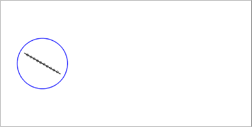
In the above,  $\Vert \cdot \Vert$ is the standard L2 (Euclidean) vector norm over the the solution vector, i.e. the square error is summed over each grid point. In the discussion below, we also introduce an error norm restricted to points away from the surface of the body, which we denote as
 $\Vert \cdot \Vert _{r}$. This error metric is introduced to be able to distinguish errors associated with forces on the immersed surface from those associated with the flow dynamics in the wake. Figure 2 illustrates the precise regions over which the full and restricted norms are defined.
Illustration of the different domains used for the evaluation of the state error. The full norm is over the entire computational domain represented by the black box; the restricted norm is defined by those points in the full domain outside the blue circle. The small circles on the surface of the plate represent the locations where the pressure measurements are taken.

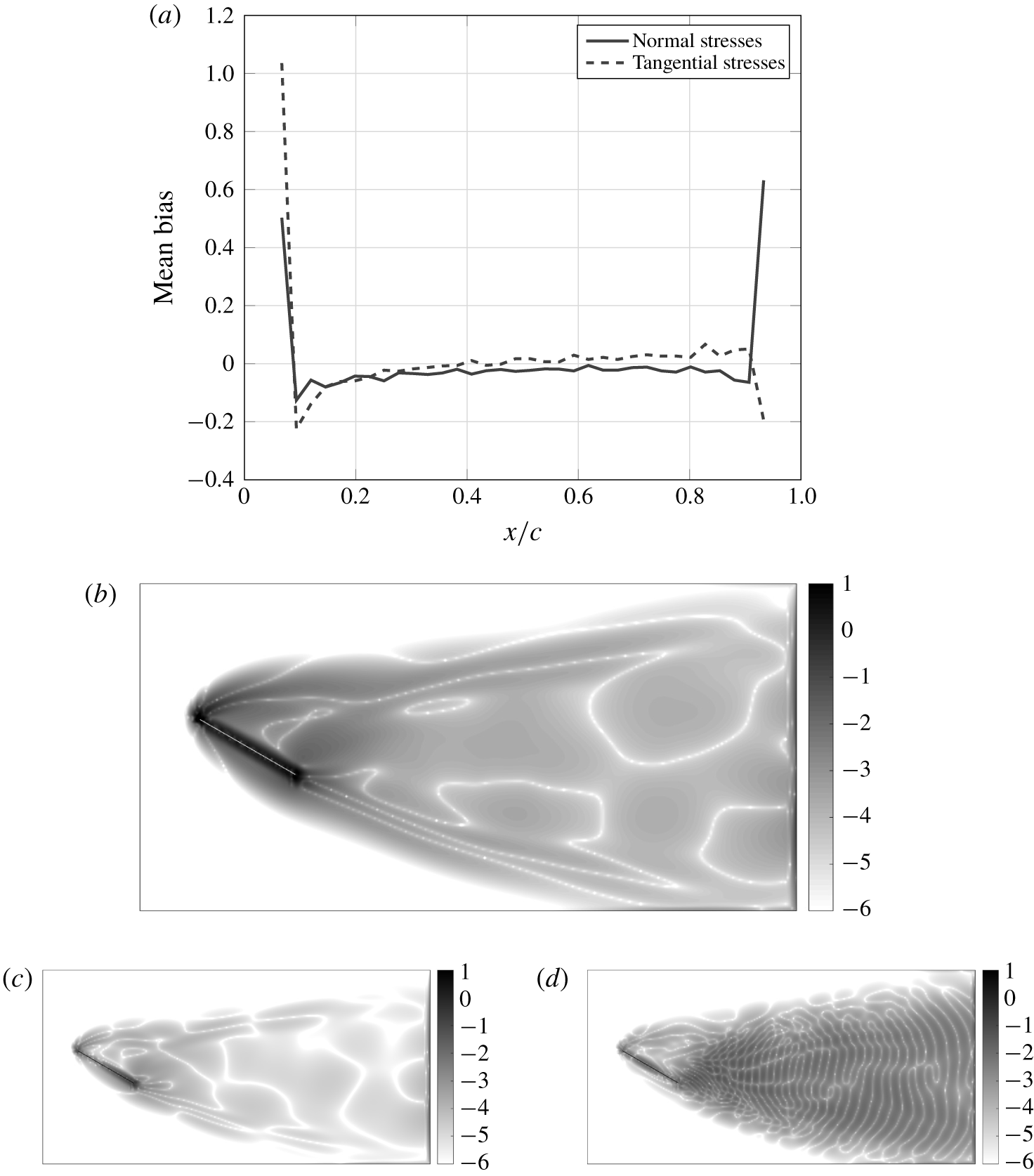
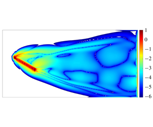
Spatial distribution of the bias fields introduced by the resolution error for the flow past an inclined flat plate when comparing the  $Re_{\unicode[STIX]{x1D6E5}}=1$ (200 grid points per chord) simulation to the corresponding
 $Re_{\unicode[STIX]{x1D6E5}}=4$ (50 grid points per chord) simulation. (a) Temporal average of the bias field for the observation model (
 $\bar{\unicode[STIX]{x1D750}}^{r}$). (b) Temporal average of the bias field for the dynamic model (
 $\bar{\unicode[STIX]{x1D739}}$) in log scale. (c) The first POD mode of the bias field for the dynamic model (
 $\boldsymbol{u}_{1}^{s}$) in log scale. (d) The 25th POD mode of the bias field for the dynamic model (
 $\boldsymbol{u}_{25}^{s}$) in log scale.

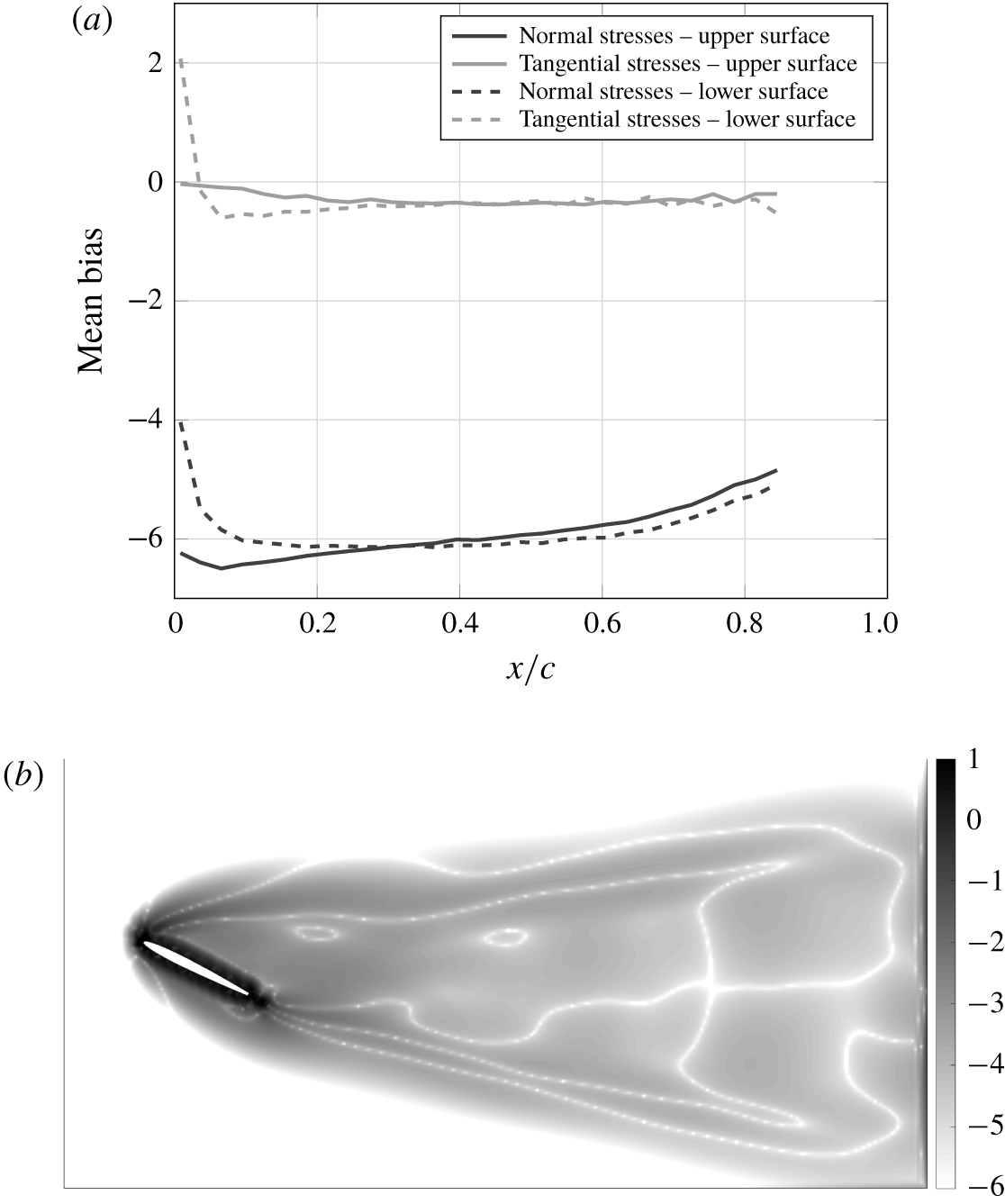
Temporal average of the bias fields introduced by the resolution error for the flow past an inclined NACA 0009 when comparing the  $Re_{\unicode[STIX]{x1D6E5}}=1$ (200 grid points per chord) simulation to the corresponding
 $Re_{\unicode[STIX]{x1D6E5}}=4$ (50 grid points per chord) simulation. (a) Bias field for the observation model (
 $\bar{\unicode[STIX]{x1D750}}^{r}$). (b) Bias field for the dynamic model (
 $\bar{\unicode[STIX]{x1D739}}$) in log scale.

5.2 Identification of the resolution error basis
The numerical error introduced by the different resolution levels is the source of the bias that we will be interested in tracking. State statistics are estimated from a set of base solutions at the different resolutions spanning a sufficiently long time window. Bias statistics can then be estimated using the definitions presented in § 2
 $$\begin{eqnarray}\displaystyle & \displaystyle \unicode[STIX]{x1D71F}=\left[\begin{array}{@{}ccc@{}}\unicode[STIX]{x1D6F1}\boldsymbol{x}_{2}^{f}-f(\unicode[STIX]{x1D6F1}\boldsymbol{x}_{1}^{f}) & \cdots \, & \unicode[STIX]{x1D6F1}\boldsymbol{x}_{n}^{f}-f(\unicode[STIX]{x1D6F1}\boldsymbol{x}_{n-1}^{f})\end{array}\right], & \displaystyle\end{eqnarray}$$
 $$\begin{eqnarray}\displaystyle & \displaystyle \bar{\unicode[STIX]{x1D739}}=\frac{1}{n-1}\unicode[STIX]{x0394}\unicode[STIX]{x1D7D9}, & \displaystyle\end{eqnarray}$$
 $$\begin{eqnarray}\displaystyle & \displaystyle \unicode[STIX]{x1D640}=\left[\begin{array}{@{}ccc@{}}\unicode[STIX]{x1D6F1}h^{f}(\boldsymbol{x}_{1}^{f})-h^{c}(\unicode[STIX]{x1D6F1}\boldsymbol{x}_{1}^{f}) & \cdots \, & \unicode[STIX]{x1D6F1}h^{f}(\boldsymbol{x}_{n}^{f})-h^{c}(\unicode[STIX]{x1D6F1}\boldsymbol{x}_{n-1}^{f})\end{array}\right], & \displaystyle\end{eqnarray}$$
 $$\begin{eqnarray}\displaystyle & \displaystyle \bar{\unicode[STIX]{x1D750}^{r}}=\frac{1}{n-1}\unicode[STIX]{x1D640}\unicode[STIX]{x1D7D9}, & \displaystyle\end{eqnarray}$$
 $f$ and
 $c$ correspond, respectively, to the fine and coarse meshes, and
 $\unicode[STIX]{x1D6F1}$ is the interpolation operator between the fine and coarse meshes.
Figures 3 and 4 show the temporal mean of the bias fields of both the dynamics ( $\unicode[STIX]{x1D739}$) and observation model (
 $\unicode[STIX]{x1D750}^{r}$) between the
 $Re_{\unicode[STIX]{x1D6E5}}=4$ and
 $Re_{\unicode[STIX]{x1D6E5}}=1$ resolution levels for the airfoil and the flat plate cases, respectively. For both cases, the mean bias in the dynamics seems to concentrate near the body, where the error introduced by the immersed boundary dominates. Regarding the observation error, for the flat plate case, the bias is restricted to the leading and trailing edges, whereas for the airfoil there is a pronounced observation bias in the entire surface. The large bias observed in the normal stresses for this case can be explained by the fact that, for a closed body, the distribution of the normal component of the forces acting on its surface is only defined up to a constant (since a constant normal force acting on an immersed body will have zero resultant).
The structure of the corresponding state and observation bias covariance matrices can be analysed through POD, i.e. we compute the left singular vectors of  $\unicode[STIX]{x1D71F}-\bar{\unicode[STIX]{x1D739}}$ and
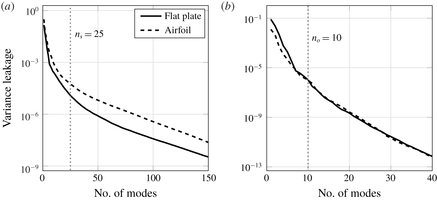
 $\unicode[STIX]{x1D640}-\bar{\unicode[STIX]{x1D750}}^{r}$, respectively. Figures 3(c) and 3(d) exemplify, respectively, a low-order and a high-order POD mode for the flat plate bias field. Note that, while the first mode qualitatively resembles the mean bias with higher magnitudes close to the body, the 25th mode displays a noisy behaviour in the wake. The low-rank bias representation proposed in § 2.1 is justified by the fact that most of the bias variance is restricted to just a few directions in the state space. Figure 5 indicates that, for the flat plate and airfoil, respectively, retaining the first
 $n_{s}=25$ state POD modes and
 $n_{o}=10$ observation POD modes leaves less than 0.01 % of the variance to be modelled as white noise.
Fraction of the bias variance left out by using the corresponding first POD modes for the flow past an inclined flat plate and a NACA 0009 airfoil. (a) State bias. (b) Observation (pressure) bias.

Therefore, matrices  $\unicode[STIX]{x1D71E}_{x}$,
 $\unicode[STIX]{x1D71E}_{y}$,
 $\bar{\unicode[STIX]{x1D743}}$ and
 $\bar{\boldsymbol{\unicode[STIX]{x1D702}}}$ in (2.8) and (2.9) can be defined as
 $$\begin{eqnarray}\displaystyle & \displaystyle \unicode[STIX]{x1D71E}_{x}=\left[\begin{array}{@{}cccc@{}}\bar{\unicode[STIX]{x1D739}} & \boldsymbol{u}_{1}^{s} & \cdots \, & \boldsymbol{u}_{n_{s}}^{s}\end{array}\right], & \displaystyle\end{eqnarray}$$
 $$\begin{eqnarray}\displaystyle & \displaystyle \unicode[STIX]{x1D71E}_{y}=\left[\begin{array}{@{}cccc@{}}\bar{\unicode[STIX]{x1D750}}^{r} & \boldsymbol{u}_{1}^{o} & \cdots \, & \boldsymbol{u}_{n_{o}}^{o}\end{array}\right], & \displaystyle\end{eqnarray}$$
 $$\begin{eqnarray}\displaystyle & \displaystyle \bar{\unicode[STIX]{x1D743}}=\bar{\boldsymbol{\unicode[STIX]{x1D702}}}=\left[\begin{array}{@{}cccc@{}}1 & 0 & \cdots \, & 0\end{array}\right]^{T}, & \displaystyle\end{eqnarray}$$
 $\boldsymbol{u}_{i}^{s}$ and
 $\boldsymbol{u}_{i}^{o}$ are the
 $i$th leading POD modes of
 $\unicode[STIX]{x1D71F}-\bar{\unicode[STIX]{x1D739}}$ and
 $\unicode[STIX]{x1D640}-\bar{\unicode[STIX]{x1D750}}^{r}$, respectively, normalized by their respective variances. The process noise
 $\unicode[STIX]{x1D741}_{k}$ is sampled from a Gaussian distribution with zero mean and covariance matrix
 $$\begin{eqnarray}\unicode[STIX]{x1D64C}_{k}=\unicode[STIX]{x1D706}\hat{\unicode[STIX]{x1D63E}}_{0}^{xx}+\left[\begin{array}{@{}ccc@{}}\boldsymbol{u}_{n_{s}+1}^{s} & \boldsymbol{u}_{n_{s}+2}^{s} & \cdots \end{array}\right]\left[\begin{array}{@{}ccc@{}}\boldsymbol{u}_{n_{s}+1}^{s} & \boldsymbol{u}_{n_{s}+2}^{s} & \cdots \end{array}\right]^{T},\end{eqnarray}$$
where  $\unicode[STIX]{x1D706}$ is a scaling factor. The auto-regressive model parameters are set to
 $\unicode[STIX]{x1D719}_{1}^{x}=\unicode[STIX]{x1D719}_{1}^{y}=\text{e}^{-\unicode[STIX]{x0394}t/\unicode[STIX]{x1D70F}}$, where
 $\unicode[STIX]{x0394}t$ is the time interval between two analysis steps, and
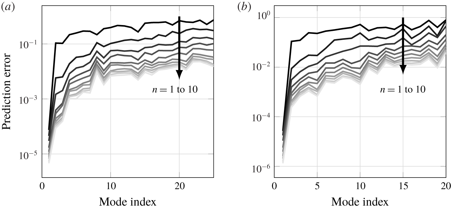
 $\unicode[STIX]{x1D70F}$ is a reference decorrelation time, here considered to be the vortex-shedding period. Alternatively, one could use a least-squares approach to determine the AR coefficients that best fit the data used to construct the low-rank model. Figure 6 shows the prediction error for the best ARn model for each of the columns of
 $\unicode[STIX]{x1D71E}_{x}$ and
 $\unicode[STIX]{x1D71E}_{y}$, where
 $n$ stands for the order of the autoregressive model. Note that the error for the first mode, the mean, is already low for the AR1 model, since its coefficient is expected to remain constant. The error for the remaining modes, however, decays slowly with increasing model order, indicating that they are more strongly time correlated. Even though the AR1 coefficients obtained via least squares differ from the initial guess based on a decorrelation time equal to the vortex-shedding period, the differences in performance of the resulting estimator were small. (Higher-order AR models were also tested as alternatives for representing the dynamics of bias. However, the resulting estimator was demonstrated to be unstable for
 $n\geqslant 2$, even though the AR models were verified to be stable themselves.)
Prediction error corresponding to the best (in a least-squares sense) ARn model for each of the POD modes selected to represent the bias. The order of the corresponding auto-regressive model increases from 1 to 10 in the direction of the arrow. (a) State bias. (b) Observation (pressure) bias.

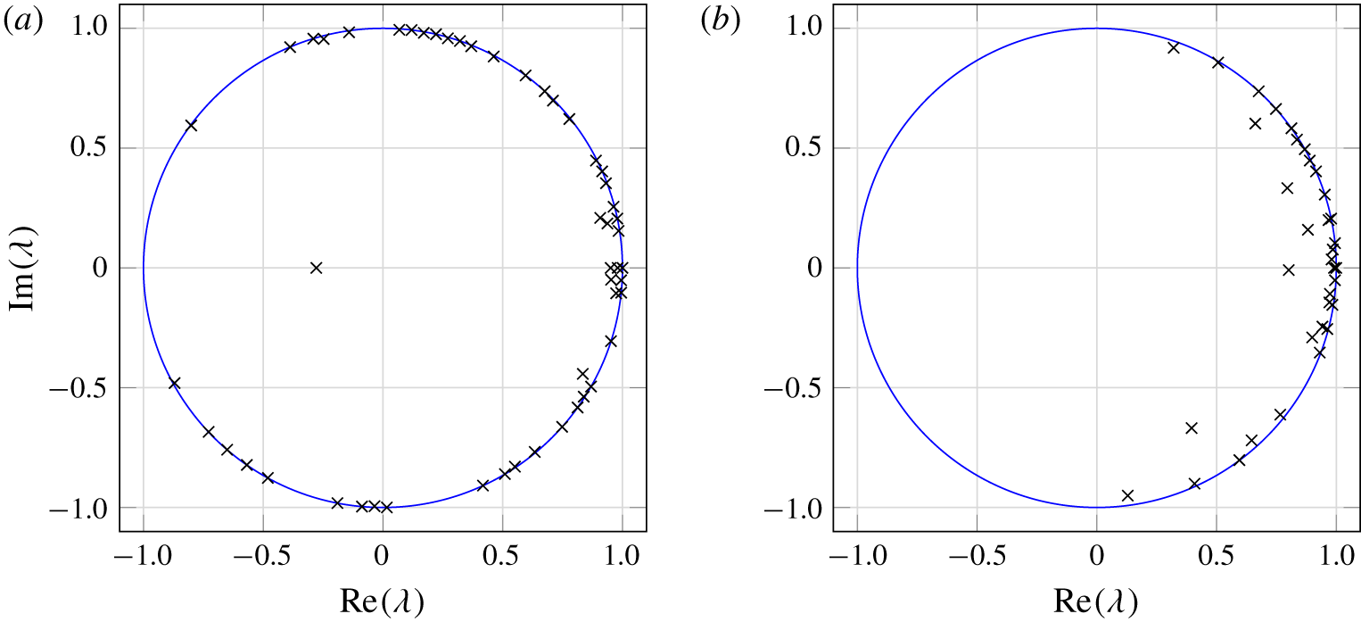
The second approach to characterizing the basis for the resolution error uses DMD (Schmid Reference Schmid2010). Each of the resulting DMD modes describes a spatial structure that evolves in time with a fixed growth/decay rate and oscillatory frequency. For a periodic phenomenon, the growth/decay rate is expected to be close to zero, i.e. the Ritz values associated with the DMD modes should lay on top of the unitary circle, as verified by figure 7. Sorting the modes by their initial magnitude, the leading modes can be selected to form the matrices  $\unicode[STIX]{x1D71E}_{x}$ and
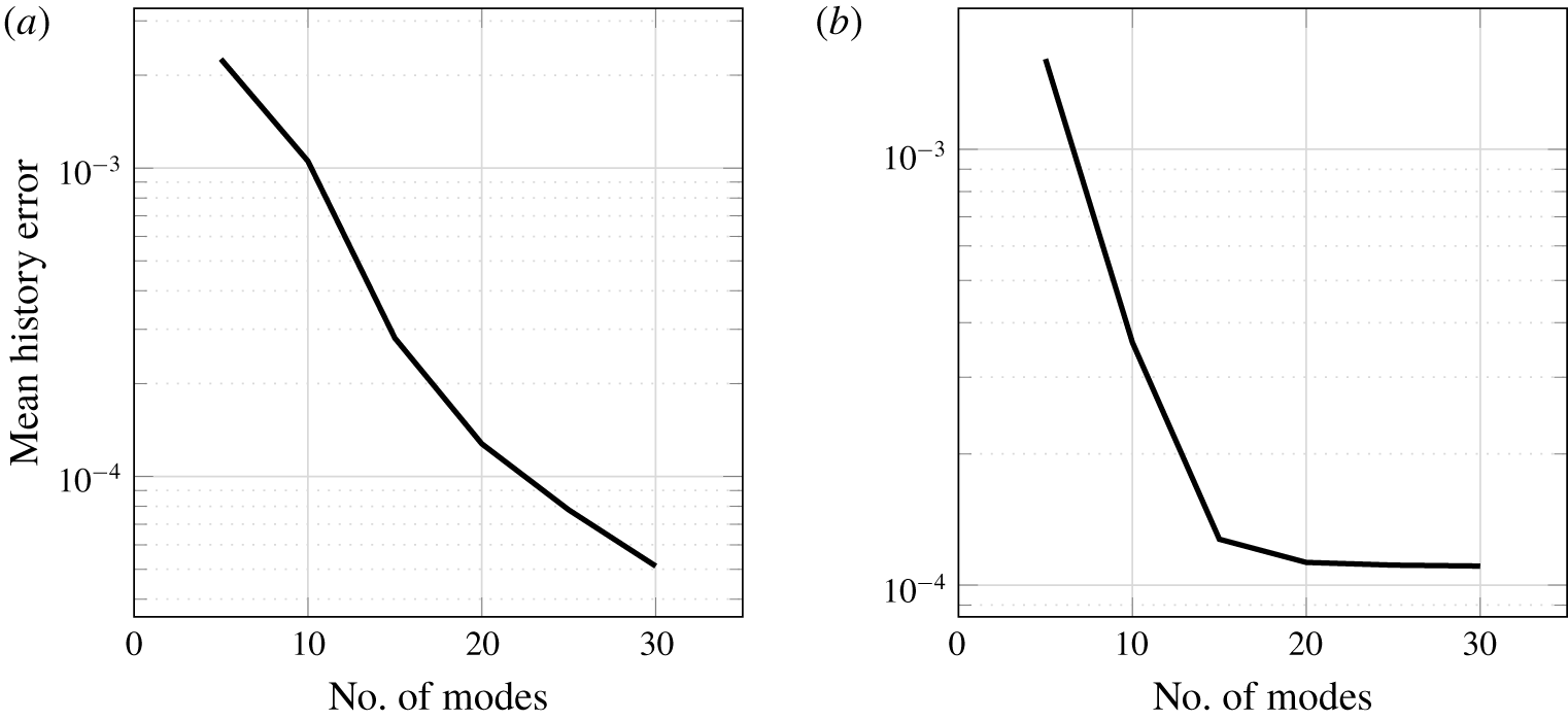
 $\unicode[STIX]{x1D71E}_{y}$. Figure 8 shows the prediction error of the low-rank model with different numbers of DMD modes when tested in the same data used to generate the DMD modes.
Ritz values corresponding to the DMD modes of the bias (when a part of a conjugate pair, only one of them is plotted). (a) State bias Ritz values. (b) Observation bias Ritz values.

Prediction error corresponding to DMD-based low-rank models with different numbers of DMD modes. (a) State bias. (b) Observation (pressure) bias.

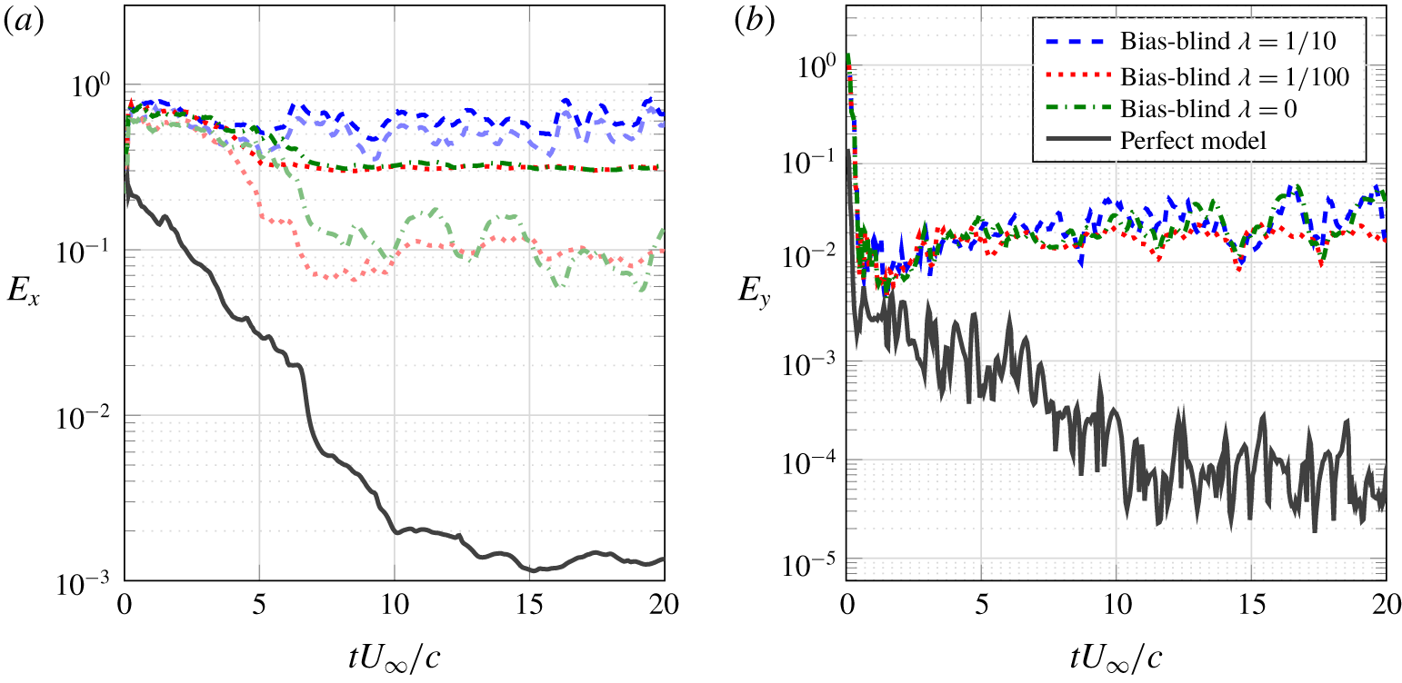
Bias-blind estimator performance highlighting the deleterious effect of the dynamics and observation bias ( $R=10^{-4}$). Darker lines correspond the standard L2 norm
 $\Vert \cdot \Vert$, while lighter lines correspond to the restricted norm
 $\Vert \cdot \Vert _{r}$. (a) State error evolution. (b) Observation error evolution.

5.3 Bias-blind estimation
In this section, we consider the case when the low-resolution model is used to track the high-resolution flat plate data without an explicit treatment of the discretization error. Rather, we use an additive covariance inflation scheme which draws its samples from a Gaussian distribution whose variance is represented by a scaled version of the initial ensemble covariance matrix (the scaling factor is represented by  $\unicode[STIX]{x1D706}$).
Figure 9 compares the performance of the bias-blind estimator for an estimator with  $Re_{\unicode[STIX]{x1D6E5}}=4$ (estimator grid is 4 times coarser than the truth) using several different magnitudes of the additive process noise. Each case is compared to the perfect model, which is an otherwise identical estimator but with
 $Re_{\unicode[STIX]{x1D6E5}}=1$, so that it matches the truth simulation. The base case (no process noise) is represented by the dash-dotted curve. While the observation error is reduced by the estimator, the state error saturates at 30 %. One can marginally improve this performance by adding just the right amount of process noise (dotted curve), but too much noise easily dominates the estimator dynamics (dashed curve). The bias-blind estimator final error is at best two orders of magnitude larger than the one that could be achieved in a perfect-model framework.
5.4 Bias-aware estimation
In this section, we evaluate the proposed bias-aware estimator when the exact flat plate bias statistics are used to form the POD-based  $\unicode[STIX]{x1D71E}$ matrices. The AR1 model is chosen to represent the dynamics of the POD coefficients. Because the proposed scheme only adds
 $n_{o}+n_{s}=35$ degrees of freedom to the much larger state vector
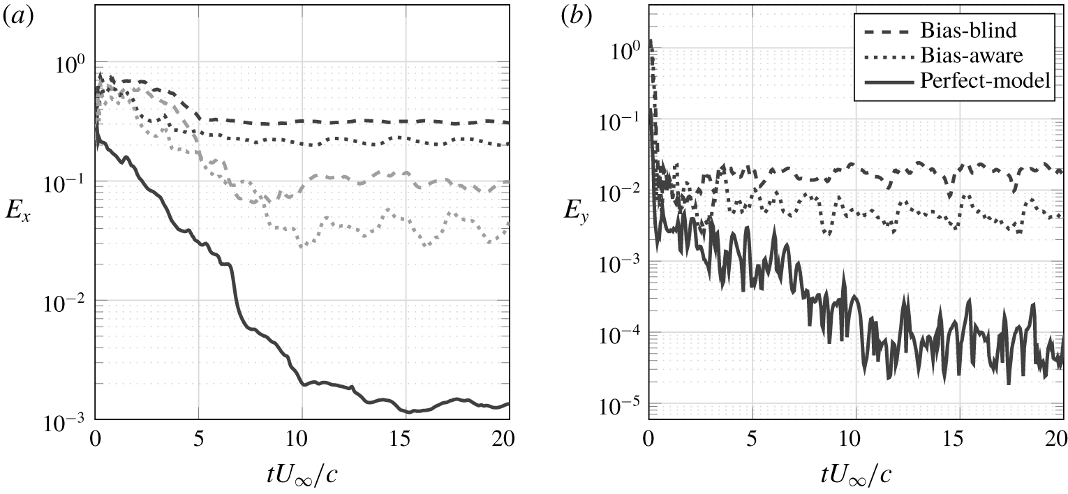
 $\boldsymbol{x}$ (approximately 15 000 degrees of freedom), the additional computational cost per ensemble member is negligible. Even though the new ensemble size is twice as big as the one used in the bias-blind framework, this additional cost can be dealt with by using extra parallel workers so that the time expenditure in the forecast step remains practically unchanged. Compared to the results from the last section, figure 10(a) shows a 33 % reduction in state error for the entire domain, while the error far from the body improves by 60 %.
Bias-aware estimator performance ( $R=10^{-4}$,
 $\unicode[STIX]{x1D706}_{o}=\sqrt{10}/10$ and
 $\unicode[STIX]{x1D706}_{s}=\sqrt{10}/10$). Black lines correspond the standard L2 norm
 $\Vert \cdot \Vert$, while grey lines correspond to the restricted norm
 $\Vert \cdot \Vert _{r}$. (a) State error evolution. (b) Observation error evolution.

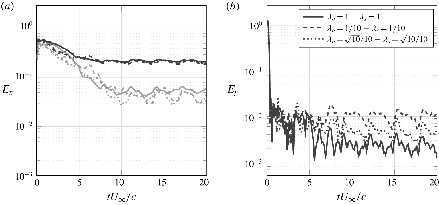
The bias dynamics is forced by process noise with covariance matrices  $\unicode[STIX]{x1D64D}^{b}=\unicode[STIX]{x1D706}_{o}\unicode[STIX]{x1D644}_{n_{o}}$ and
 $\unicode[STIX]{x1D64C}^{b}=\unicode[STIX]{x1D706}_{s}\unicode[STIX]{x1D644}_{n_{s}}$. The existence of process noise leads to a sustainably larger variance for the bias parameters, which allows for correction to be consistently made throughout the estimation window. This feature is especially important for problems like the present one, in which the bias cannot be considered as slowly varying. In fact, the bias is expected to exhibit a periodic behaviour as the flow itself is periodic with the vortex-shedding period being the fundamental time scale. Figure 11 shows how different choices of the noise magnitudes impact the state and observation error estimates. Larges values for the noise parameters favour smaller measurement mismatches (by allowing more aggressive analysis) at the expense of a possibly larger state error.
Effect of the magnitude of the process noise on bias dynamics ( $R=10^{-4}$). Black lines correspond the standard L2 norm
 $\Vert \cdot \Vert$, while grey lines correspond to the restricted norm
 $\Vert \cdot \Vert _{r}$. (a) State error evolution. (b) Observation error evolution.

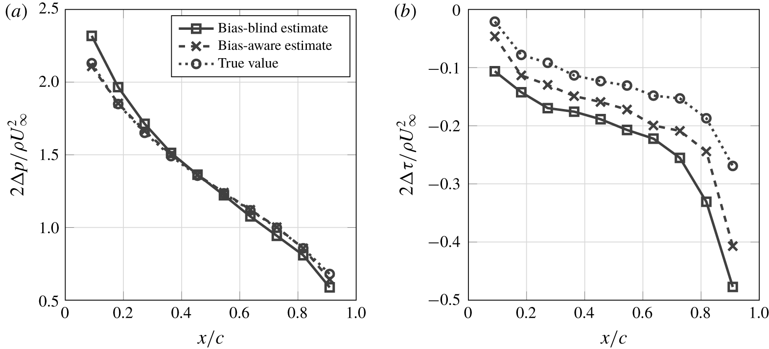
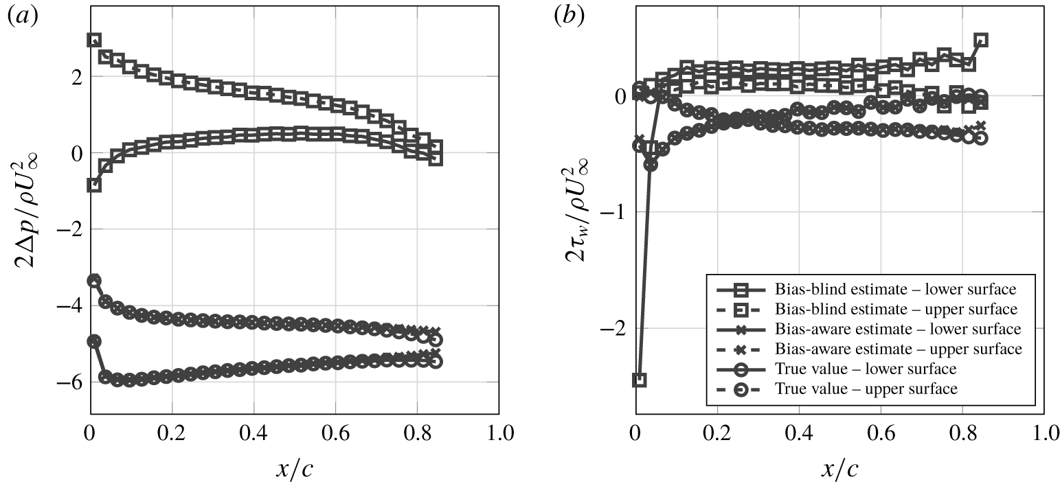
As figure 10(b) indicates, bias correction decreases the pressure error by 80 %. Figure 12 displays an example of the correction introduced by the proposed scheme to the estimated output. Correction seems to be less effective near the leading edge, possibly because of the large pressure gradients that appear in these regions. As a consequence, global quantities like the lift coefficient also have their estimates improved.
Estimated stresses on the surface of the flat plate at end of a simulation window ( $tU_{\infty }/c=20$). (a) Normal stresses. (b) Tangential stresses.

5.5 Imperfect bias statistics
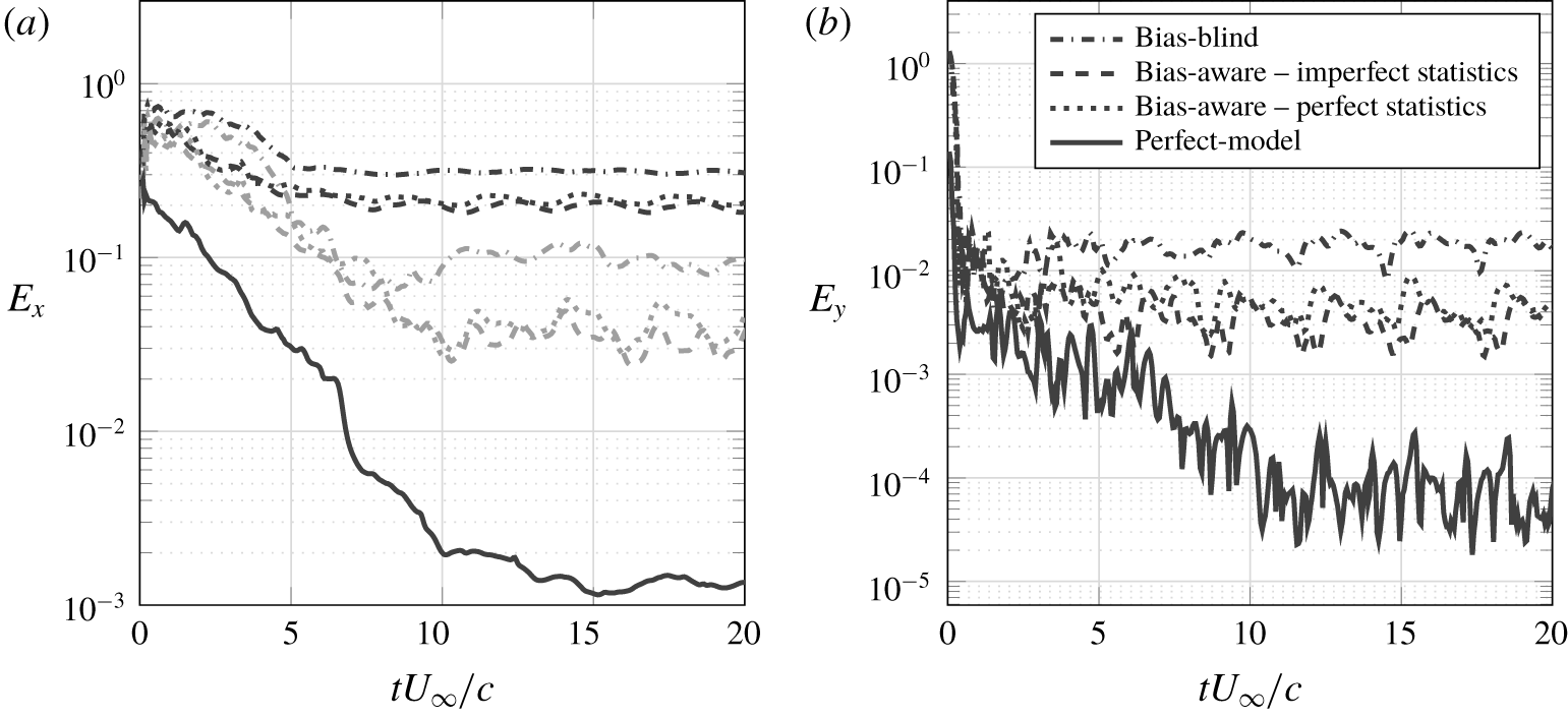
In any real application, the full state error between the estimator and truth is unknown. Since our bias model is informed by this error, we must be able to estimate it from data that are practically available. In this section, we show that estimates of the bias based on an intermediate resolution of  $Re_{\unicode[STIX]{x1D6E5}}=2$ are a sufficient surrogate for the true error (
 $Re_{\unicode[STIX]{x1D6E5}}=1$). The performance of the resulting estimator is shown in figure 13, and is similar to the one obtained with the exact statistics. This seems to indicate that, as long as one can estimate the structure of the bias, explicitly tracking it is beneficial for the estimation.
Bias-aware estimator performance with imperfect statistics ( $R=10^{-4}$). Black lines correspond to the mean-square error evaluated in the entire computational domain, while the grey lines restrict this evaluation to the region outside a unit circle centred at the plate. (a) State error evolution. (b) Observation error evolution.

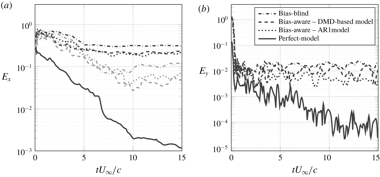
Effect of different choices of models for the bias dynamics on the performance of the bias-aware estimator. Black lines correspond the standard L2 norm  $\Vert \cdot \Vert$, while grey lines correspond to the restricted norm
 $\Vert \cdot \Vert _{r}$. (a) State error evolution. (b) Observation error evolution.

5.6 POD-AR-based versus DMD-based bias models
We now address the effect of different choices of models for the bias dynamics on the performance of the bias-aware estimator. Figure 14 compares the POD-AR1 estimator presented in the previous sections with the DMD-based estimator. Recalling figure 8, we use 12 DMD modes to represent the observation bias and 18 DMD modes to represent the state forecast bias, which makes the cost comparable to the POD-AR1 model set-up. In terms of state error, both estimators have comparable performance, but the DMD-based estimator delivers poorer estimates for the estimated measurements.
Since this flow is essentially periodic, it was expected that the harmonic model would be a better representation of the bias dynamics. Thus, if the analysis were able to apply a correction to the state that would bring it close to the actual state, we would expect that the error introduced by the dynamics would be smaller when the harmonic model is used than when the AR-based model is used, leading to an improved overall performance of the estimator. However, results show little influence of the bias dynamics model on the estimator performance. This seems to indicate that the suboptimality in the analysis step is the dominant source of estimation error in this case.
5.7 Airfoil case
Next, we present the results of applying the bias-aware methodology to the more stringent airfoil case where, as was shown in § 5.2, the discretization bias is more pronounced compared to the flat plate. Again, we model the bias dynamics using the POD-AR1 model (with the same number of modes as before). Figure 15 shows that the bias-aware estimator greatly improves the accuracy throughout the entire estimation window, achieving a long-term error reduction of 85 % for the state and 90 % for the measurements. Figure 16 compares the estimated measurements to their real values before assimilation. The bias scheme is able to successfully correct the stresses on the surface of the airfoil. It can be noted, however, that most of the persistent error is located near the trailing edge.
Bias-aware estimator performance ( $R=10^{-4}$,
 $\unicode[STIX]{x1D706}_{o}=1/10$ and
 $\unicode[STIX]{x1D706}_{s}=1$) for the inclined NACA 0009 problem. Black lines correspond the standard L2 norm
 $\Vert \cdot \Vert$, while grey lines correspond to the restricted norm
 $\Vert \cdot \Vert _{r}$. (a) State error evolution. (b) Observation error evolution.

Estimated stresses on the surface of the NACA 0009 at the end of a simulation window ( $tU_{\infty }/c=30$). (a) Normal stresses. (b) Tangential stresses.

6 Conclusions
In this paper, we introduced an approach to use an EnKF framework to simultaneously mitigate the effects of biased forecast and observation models resulting from coarse discretization of the flow. In lieu of treating the bias as a single random variable, we split it into slow and fast components. The fast (incoherent) component was treated as temporally uncorrelated white noise with a specified covariance, and it can therefore be absorbed in an additive covariance inflation (process noise) scheme.
The slow (coherent) part is represented in a low-rank subspace of the measured error between simulations at different grid resolutions. The subspace was determined by either POD or DMD. The time-correlated modal amplitudes were modelled as an auto-regressive process in the case of POD, or by a harmonic process with the corresponding Ritz value in the case of DMD. The restriction of the bias dynamics to the low-rank subspace that contains most of the variance allows for a more efficient sampling of the state space and enables the use of fewer ensemble members to satisfactorily represent the system statistics. In the examples we considered, the AR- and DMD-based models performed similarly, indicating that the error introduced by a suboptimal analysis is the dominant source of error in this case, as discussed in § 5.6.
The performance of the proposed estimator was assessed by employing an ensemble of coarse-grid simulations to track a fine-grid simulation of the low- $Re$ flow past a flat plate and an airfoil at high angle of attack. Measurement data consisted of pressure at ten different locations on the surface. Because the pressure is a nonlinear function of the vorticity field, Evensen’s implicit linearization scheme was employed. For a small cost increment, the bias-aware estimator reduced the state and observation error by 70 % for the flat plate and 80 % for the airfoil, compared to the bias-blind scheme, and by even larger percentages for the airfoil case where the uncorrected discretization bias was higher. The improvement was similar when the exact error between the truth and the estimator was used to inform the bias statistics, and when the value was inferred by extrapolation from databases with differing intermediate resolutions. Thus the scheme could be used with real measurement data and error data collected a priori by running the model at different resolutions.
The requirement of a prior representation of the bias statistics can be viewed as a limitation of the present method, and a methodology that forgoes the need for a priori statistics would be very welcome. A very promising direction points towards multi-fidelity estimators, which intend to leverage information obtained from different models (each of them with their own strengths and fragilities) to optimize the ratio accuracy/cost (Peherstorfer, Willcox & Gunzburger Reference Peherstorfer, Willcox and Gunzburger2018). Along these lines, multilevel Monte Carlo methods (Giles Reference Giles2015; Hoel et al. Reference Hoel, Law and Tempone2016) have been showing interesting results, employing a sequence of models of increasing complexity. We believe such techniques could be fruitfully combined in the EnKF framework. Finally, a logical next step would be the application of this methodology to more complex flows, especially those there is more slow/fast separation of scales and/or more coherent/incoherent motion would provide a valuable test for the bias models.
Acknowledgements
This study has been supported in part by a grant from AFOSR (FA9550-14-1-0328) with Dr D. Smith as program manager, and in part by the Coordenação de aperfeiçoamento de Pessoal de Nível Superior – Brasil (CAPES) – Finance Code 001 (grant no. BEX 12966/13-4). The authors also acknowledge Professors D. Williams (Illinois Institute of Technology), J. Eldredge (UCLA) and A. Stuart (Caltech) for helpful discussions of this work.
Declaration of interests
The authors report no conflict of interests.
Appendix A. EnKF algorithm
The standard EnKF algorithm can be summarized as follows:

Appendix B. A variational approach to the EnKF
Following the variational approach, the ensemble members are corrected in order to minimize the error with respect to the measurements in the presence of noise and model uncertainties. In other words, we look for the minimizer of the cost function
 $$\begin{eqnarray}\displaystyle J(\boldsymbol{x}) & = & \displaystyle \frac{1}{2\unicode[STIX]{x1D6FC}}\Vert \boldsymbol{x}-\hat{\boldsymbol{x}}_{k}^{(j)}\Vert _{\hat{\unicode[STIX]{x1D63E}}_{k}}^{2}+\frac{1}{2}\Vert \boldsymbol{y}_{k}-\unicode[STIX]{x1D643}\boldsymbol{x}\Vert _{\unicode[STIX]{x1D64D}}^{2}\nonumber\\ \displaystyle & = & \displaystyle \frac{1}{2\unicode[STIX]{x1D6FC}}[\boldsymbol{x}-\hat{\boldsymbol{x}}_{k}^{(j)}]^{T}\hat{\unicode[STIX]{x1D63E}}_{k}^{-1}[\boldsymbol{x}-\hat{\boldsymbol{x}}_{k}^{(j)}]+\frac{1}{2}[\boldsymbol{y}_{k}-\unicode[STIX]{x1D643}\boldsymbol{x}]^{T}\unicode[STIX]{x1D64D}^{-1}[\boldsymbol{y}_{k}-\unicode[STIX]{x1D643}\boldsymbol{x}].\end{eqnarray}$$
The parameter  $\unicode[STIX]{x1D6FC}$ in the cost function represents a multiplicative covariance inflation (CI) (Anderson & Anderson Reference Anderson and Anderson1999). When finite ensemble sizes are used, EnKF analysis systematically underestimates error covariance (van Leeuwen Reference van Leeuwen1999). Left unattended, this fact can lead to covariance collapse, where each ensemble member predicts the same (possibly incorrect) dynamics. Taking
 $\unicode[STIX]{x1D6FC}>1$ artificially increases the ensemble covariance in order to weight the measurement data more heavily. This simple CI approach is equivalent to introducing a process noise whose covariance matrix is given by the prior ensemble covariance matrix scaled by
 $\unicode[STIX]{x1D6FC}^{2}$. A more general CI scheme can be implemented as
 $$\begin{eqnarray}\hat{\boldsymbol{x}}_{adj}^{(j)}=\bar{\boldsymbol{x}}+\unicode[STIX]{x1D736}(\hat{\boldsymbol{x}}^{(j)}-\bar{\boldsymbol{x}})+\unicode[STIX]{x1D737}^{(j)},\end{eqnarray}$$
where  $\unicode[STIX]{x1D737}^{(j)}$ is the additive covariance inflation vector that is usually drawn from a zero-mean normal distribution with a predefined covariance matrix, and
 $\unicode[STIX]{x1D736}$ is the multiplicative covariance inflation parameter. Multiplicative CI is used to correct the filter transient behaviour by delaying the collapse of the covariance, while additive CI will enforce a lower bound to the system covariance, limiting its perceived reliability. In more sophisticated CI schemes,
 $\unicode[STIX]{x1D736}$ and
 $\unicode[STIX]{x1D737}$ can be a matrix and vector, respectively (Whitaker & Hamill Reference Whitaker and Hamill2012). Note also that, although used for different purposes, additive covariance inflation is algorithmically equivalent to process noise as both are implemented by adding perturbations to each of the ensemble members that are sampled from a prescribed probability distribution.
This optimization problem is then restricted to the affine space generated by the prior estimate of each of the ensemble members and the subspace spanned by the scaled perturbation matrix  $\hat{\unicode[STIX]{x1D63C}}_{k}$. In other words, we look for a solution in the form
 $$\begin{eqnarray}\boldsymbol{x}=\hat{\boldsymbol{x}}_{k}^{(j)}+\sqrt{\unicode[STIX]{x1D6FC}}\hat{\unicode[STIX]{x1D63C}}_{k}\boldsymbol{v},\end{eqnarray}$$
where  $\boldsymbol{v}\in \mathbb{R}^{q}$ is the correction coefficient vector.
After performing the proposed change of variables, we can restate the objective of the analysis step as finding
 $$\begin{eqnarray}\boldsymbol{v}=\underset{\boldsymbol{v}\in \mathbb{R}^{q}}{\text{arg}\,\text{min}}~J(\boldsymbol{v})\end{eqnarray}$$
for each of the ensemble members, where
 $$\begin{eqnarray}J(\boldsymbol{v})={\textstyle \frac{1}{2}}\Vert \boldsymbol{v}\Vert ^{2}+{\textstyle \frac{1}{2}}\Vert \boldsymbol{y}_{k}-\unicode[STIX]{x1D643}\hat{\boldsymbol{x}}_{k}^{(j)}-\sqrt{\unicode[STIX]{x1D6FC}}\unicode[STIX]{x1D643}\hat{\unicode[STIX]{x1D63C}}_{k}\boldsymbol{v}\Vert _{\unicode[STIX]{x1D64D}}^{2}.\end{eqnarray}$$
Since  $J(\boldsymbol{v})$ is quadratic in
 $\boldsymbol{v}$, the solution is unique and corresponds to the root of
 $$\begin{eqnarray}\boldsymbol{D}\boldsymbol{J}(\boldsymbol{v})=\boldsymbol{v}-(\sqrt{\unicode[STIX]{x1D6FC}}\unicode[STIX]{x1D643}\hat{\unicode[STIX]{x1D63C}}_{k})^{T}\unicode[STIX]{x1D64D}^{-1}(\boldsymbol{y}_{k}-\unicode[STIX]{x1D643}\hat{\boldsymbol{x}}_{k}^{(j)}-\sqrt{\unicode[STIX]{x1D6FC}}\unicode[STIX]{x1D643}\hat{\unicode[STIX]{x1D63C}}_{k}\boldsymbol{v})=0,\end{eqnarray}$$
which is given by
 $$\begin{eqnarray}\displaystyle \boldsymbol{v}_{k}^{(j)} & = & \displaystyle \sqrt{\unicode[STIX]{x1D6FC}}[\unicode[STIX]{x1D644}+\unicode[STIX]{x1D6FC}(\unicode[STIX]{x1D643}\hat{\unicode[STIX]{x1D63C}}_{k})^{T}\unicode[STIX]{x1D64D}^{-1}(\unicode[STIX]{x1D643}\hat{\unicode[STIX]{x1D63C}}_{k})]^{-1}(\unicode[STIX]{x1D643}\hat{\unicode[STIX]{x1D63C}}_{k})^{T}\unicode[STIX]{x1D64D}^{-1}(\boldsymbol{y}_{k}-\unicode[STIX]{x1D643}\hat{\boldsymbol{x}}_{k}^{(j)})\end{eqnarray}$$
 $$\begin{eqnarray}\displaystyle & = & \displaystyle \sqrt{\unicode[STIX]{x1D6FC}}(\unicode[STIX]{x1D643}\hat{\unicode[STIX]{x1D63C}}_{k})^{T}[\unicode[STIX]{x1D64D}+\unicode[STIX]{x1D6FC}(\unicode[STIX]{x1D643}\hat{\unicode[STIX]{x1D63C}}_{k})(\unicode[STIX]{x1D643}\hat{\unicode[STIX]{x1D63C}}_{k})^{T}]^{-1}(\boldsymbol{y}_{k}-\unicode[STIX]{x1D643}\hat{\boldsymbol{x}}_{k}^{(j)}),\end{eqnarray}$$
The final solution ((3.7a) and (3.7b)) is then obtained by projecting these coefficients back to the state space.
Other than the covariance inflation, localization (Houtekamer & Mitchell Reference Houtekamer and Mitchell2001) is a second heuristic that is commonly used in ensemble methods to reduce the negative side effects associated with a reduced ensemble size. Localization schemes are based on the premise that the correlation between two points in the domain should decrease as the distance between them increases, and artificially suppress the off-diagonal components of the covariance matrix  $\unicode[STIX]{x1D63E}_{k}$ in order to mitigate spurious correlations due to undersampling. While such a methodology proved very useful for turbulent flows (see Colburn et al. (Reference Colburn, Cessna and Bewley2011), for instance), that is not the case here. Low-
 $Re$ flows past bluff bodies, like the ones studied in this work, display longstanding coherent structures in the wake and, therefore, display long-distance correlations that are not spurious but are in fact physical.
Both the particle filter (PF) and the EnKF algorithms share the same forecast step, but their analysis steps are distinct. While in the PF the posterior probability density function corresponds to a linear combination of the prior ensemble whose weights are calculated using the Bayes rule, the EnKF assign equal weights to all particles and correct the ensemble members themselves according to Kalman’s update rule (Colburn et al. Reference Colburn, Cessna and Bewley2011). Because the particles themselves are driven towards the measurements, the need for resampling is eliminated.
Appendix C. Implicit linearization
The scheme proposed by Evensen (Reference Evensen2009) to deal with nonlinear observation functions can be understood as an approximate linearization about the ensemble-averaged state. To see this, notice that each of the columns of  $\unicode[STIX]{x1D647}\tilde{\unicode[STIX]{x1D642}}\hat{\unicode[STIX]{x1D63C}}_{k}$ is given by
 $$\begin{eqnarray}\displaystyle \sqrt{q-1}\{\unicode[STIX]{x1D647}\hat{\unicode[STIX]{x1D63D}}^{w}\}_{j} & = & \displaystyle h^{\dagger }(\unicode[STIX]{x1D642}\,\hat{\boldsymbol{z}}_{k}^{(j)})-\frac{1}{q}\mathop{\sum }_{i=1}^{q}h^{\dagger }(\unicode[STIX]{x1D642}\,\hat{\boldsymbol{z}}_{k}^{(i)})\nonumber\\ \displaystyle & = & \displaystyle h^{\dagger }(\unicode[STIX]{x1D642}\,\hat{\boldsymbol{z}}_{k}^{(j)})-\frac{1}{q}\mathop{\sum }_{i=1}^{q}\left[h^{\dagger }(\unicode[STIX]{x1D642}\,\bar{\hat{\boldsymbol{z}}}_{k})+\frac{\unicode[STIX]{x2202}h^{\dagger }}{\unicode[STIX]{x2202}\boldsymbol{z}}(\unicode[STIX]{x1D642}\,\bar{\hat{\boldsymbol{z}}}_{k})\unicode[STIX]{x1D642}(\hat{\boldsymbol{z}}_{k}^{(j)}-\bar{\hat{\boldsymbol{z}}}_{k})+O[(\hat{\boldsymbol{z}}_{k}-\bar{\hat{\boldsymbol{z}}}_{k})^{2}]\right]\nonumber\\ \displaystyle & = & \displaystyle h^{\dagger }(\unicode[STIX]{x1D642}\,\hat{\boldsymbol{z}}_{k}^{(j)})-h^{\dagger }(\unicode[STIX]{x1D642}\,\bar{\hat{\boldsymbol{z}}}_{k})+O[(\hat{\boldsymbol{z}}_{k}-\bar{\hat{\boldsymbol{z}}}_{k})^{2}]\nonumber\\ \displaystyle & = & \displaystyle \frac{\unicode[STIX]{x2202}h^{\dagger }}{\unicode[STIX]{x2202}\boldsymbol{z}}(\unicode[STIX]{x1D642}\,\bar{\hat{\boldsymbol{z}}}_{k})\unicode[STIX]{x1D642}(\hat{\boldsymbol{z}}_{k}^{(j)}-\bar{\hat{\boldsymbol{z}}}_{k})+O[(\hat{\boldsymbol{z}}_{k}-\bar{\hat{\boldsymbol{z}}}_{k})^{2}]\end{eqnarray}$$
 $$\begin{eqnarray}\displaystyle \hat{\unicode[STIX]{x1D63E}}_{k}^{yy} & = & \displaystyle \frac{1}{q-1}\mathop{\sum }_{j=1}^{q}\left(h^{\dagger }(\unicode[STIX]{x1D642}\,\hat{\boldsymbol{z}}_{k}^{(j)})-\frac{1}{q}\mathop{\sum }_{i=1}^{q}h^{\dagger }(\unicode[STIX]{x1D642}\,\hat{\boldsymbol{z}}_{k}^{(i)})\right)\left(h^{\dagger }(\unicode[STIX]{x1D642}\,\hat{\boldsymbol{z}}_{k}^{(j)})-\frac{1}{q}\mathop{\sum }_{i=1}^{q}h^{\dagger }(\unicode[STIX]{x1D642}\,\hat{\boldsymbol{z}}_{k}^{(i)})\right)^{T}\nonumber\\ \displaystyle & = & \displaystyle \left[\frac{\unicode[STIX]{x2202}h^{\dagger }}{\unicode[STIX]{x2202}\boldsymbol{z}}(\unicode[STIX]{x1D642}\,\bar{\hat{\boldsymbol{z}}}_{k})\right]\!\unicode[STIX]{x1D642}\left(\frac{1}{q-1}\mathop{\sum }_{j=1}^{q}(\hat{\boldsymbol{z}}_{k}^{(j)}-\bar{\hat{\boldsymbol{z}}}_{k})(\hat{\boldsymbol{z}}_{k}^{(j)}-\bar{\hat{\boldsymbol{z}}}_{k})^{T}\right)\!\unicode[STIX]{x1D642}^{T}\left[\frac{\unicode[STIX]{x2202}h^{\dagger }}{\unicode[STIX]{x2202}\boldsymbol{z}}(\unicode[STIX]{x1D642}\,\bar{\hat{\boldsymbol{z}}}_{k})\right]^{T}+O[(\hat{\boldsymbol{z}}_{k}-\bar{\hat{\boldsymbol{z}}}_{k})^{3}]\nonumber\\ \displaystyle & = & \displaystyle \left[\frac{\unicode[STIX]{x2202}h^{\dagger }}{\unicode[STIX]{x2202}\boldsymbol{z}}(\unicode[STIX]{x1D642}\,\bar{\hat{\boldsymbol{z}}}_{k})\right]\unicode[STIX]{x1D642}\,\hat{\unicode[STIX]{x1D63E}}_{k}^{zz}\unicode[STIX]{x1D642}^{T}\left[\frac{\unicode[STIX]{x2202}h^{\dagger }}{\unicode[STIX]{x2202}\boldsymbol{z}}(\unicode[STIX]{x1D642}\,\bar{\hat{\boldsymbol{z}}}_{k})\right]^{T}+O[(\hat{\boldsymbol{z}}_{k}-\bar{\hat{\boldsymbol{z}}}_{k})^{3}],\end{eqnarray}$$
and
 $$\begin{eqnarray}\hat{\unicode[STIX]{x1D63E}}_{k}^{zy}=\hat{\unicode[STIX]{x1D63E}}_{k}^{zz}\unicode[STIX]{x1D642}^{T}\left[\frac{\unicode[STIX]{x2202}h^{\dagger }}{\unicode[STIX]{x2202}\boldsymbol{z}}(\bar{\hat{\boldsymbol{z}}}_{k})\right]^{T}+O[(\hat{\boldsymbol{z}}_{k}-\bar{\hat{\boldsymbol{z}}}_{k})^{3}].\end{eqnarray}$$
These approximations are consistent with the approximate minimization of an effective cost function
 $$\begin{eqnarray}J(\boldsymbol{z})=\frac{1}{2\unicode[STIX]{x1D6FC}}\Vert \tilde{\unicode[STIX]{x1D642}}^{-1}\boldsymbol{z}-\hat{\boldsymbol{z}}_{k}^{(j)}\Vert _{\hat{\unicode[STIX]{x1D63E}}^{zz}}^{2}+\frac{1}{2}\left\Vert \boldsymbol{y}_{k}-h^{\dagger }(\unicode[STIX]{x1D642}\,\bar{\hat{\boldsymbol{z}}})-\left[\frac{\unicode[STIX]{x2202}h^{\dagger }}{\unicode[STIX]{x2202}\boldsymbol{z}}(\unicode[STIX]{x1D642}\,\bar{\hat{\boldsymbol{z}}})\right](\boldsymbol{z}-\unicode[STIX]{x1D642}\,\bar{\hat{\boldsymbol{z}}})-\unicode[STIX]{x1D742}_{k}^{(j)}\right\Vert _{\unicode[STIX]{x1D64D}}^{2},\end{eqnarray}$$
which corresponds to the cost function of an extended Kalman filter in which the linearization is performed about the ensemble average instead of the prior state of the particle.