1 Introduction
Understanding the partial or total collapse of dams and the resulting fluid flow is vital for the protection of people, infrastructure and environment downstream. When a dam fails, it is common for only a portion of it to collapse, creating an obstacle for the upstream reservoir to navigate before it rushes downstream. This results in a gravity current, where the horizontal density difference between the current and ambient fluid drives the flow (Simpson Reference Simpson1997; Ungarish Reference Ungarish2009). The investigation into gravity currents has a long history (von Kármán Reference von Kármán1940) due to their many industrial and environmental applications, including open channel hydraulics, ventilation, the spreading of toxic gas, intrusion of saline water in estuaries and chemical and oil spillage. Important fundamental problems in this research area include ‘dam-break’ and ‘lock-release’ flows, in which initially quiescent fluid held behind a barrier, surrounded by a lower density ambient, is suddenly released to flow along a channel. The term ‘lock release’ usually relates to Boussinesq flows for which the density ratio between the current and ambient is order unity, whereas the term ‘dam break’ is often used for non-Boussinesq flows in this configuration, importantly including the subaerial collapse of a fluid reservoir. These flows are not only important for their applications, but are well established experiments in laboratory settings as documented by Simpson (Reference Simpson1982) and Ungarish (Reference Ungarish2009), including flows interacting with barriers (Lane-Serff, Beal & Hadfield Reference Lane-Serff, Beal and Hadfield1995; Wilson, Friedrich & Stevens Reference Wilson, Friedrich and Stevens2017). The motion is non-trivial because the dynamics evolves spatially and temporally, and yet the configuration is sufficiently simple to allow the fundamental fluid mechanical mechanisms to be clearly investigated.
When modelling gravity currents and other free-surface hydraulic flows, their extreme aspect ratio is exploited, as the motion typically has vastly greater horizontal extent than depth. This asymptotic regime gives rise to a hydrostatic pressure field, and thence the shallow water equations can be deduced (Ungarish Reference Ungarish2009). Around the flow head where the current propagates into the ambient, however, hydrostatic pressure is not an accurate approximation, and special considerations must be made. Benjamin (Reference Benjamin1968) performed one of the first comprehensive investigations into the steady dynamics of the head for two layer flows in a lidded channel, and established conditions of the form
 $u=Fr\sqrt{gh}$
relating the velocity of head
 $u$
to gravitational acceleration
 $g$
and the depth of upstream flow
 $h$
by the Froude number
 $Fr$
, where the Froude number is a function of both the ratio of the flow depth to the channel height, and the ratio of the current to ambient densities. This work has been recently revisited by Ungarish & Hogg (Reference Ungarish and Hogg2018) to account for the vorticity developed by the flow as it overpasses the front. Solutions for unsteady dam-break and lock-release flows have been constructed by employing the Froude number condition as a dynamical boundary condition for the shallow water equations at the front of the motion (Rottman & Simpson Reference Rottman and Simpson1983). From lock-release initial conditions, the current rapidly accelerates to propagate with constant velocity (Ungarish Reference Ungarish2009) before entering a self-similar regime in which the inertia of the fluid motion is in balance with the hydrostatic pressure gradients (Fannelop & Waldman Reference Fannelop and Waldman1972; Hoult Reference Hoult1972). The approach to self-similarity is characterised by interfacial waves that propagate between the front of the current and the back wall of the reservoir (Hogg Reference Hogg2006).
Despite the extensive investigation into dam-break flows, there are many important variations that have not been studied. In this work we consider the possibility of incomplete breakage of a dam, either by collapse of the upper portions, creating a weir, or the centre portion, creating a constriction. A similar situation occurs with the sudden (partial) opening of a sluice gate in a canal. Broad-crested weirs (BCW), where the horizontal crest extends for a sufficient length such that critical flow with hydrostatic pressure is established (Chow Reference Chow2009), are of particular interest here. Early work on this topic was documented by Horton (Reference Horton1907) for sharp-edged BCW, in which the flux of fluid over the weir is related by empirical relationships to upstream flow characteristics. Whilst many different empirical relationships are still in use, the one presented Ackers et al. (Reference Ackers, White, Perkins and Harrison1978) is useful for conceptual understanding as it uses a drainage coefficient
 $C_{d}$
which can be related to the ratio of upstream energy head
 $H_{u}$
to crest energy head
 $H_{c}$
(using the crest height as the datum) as
 $H_{c}/H_{u}=C_{d}^{2/3}$
. Values of
 $C_{d}$
are calculated from data compiled from 18 different studies in Zachoval et al. (Reference Zachoval, Knéblová, Rous̆ar, Rumann and S̆ulc2014) and from their results we calculate a head loss of
 $3\,\%$
–
 $12\,\%$
. Experimental results for a variety of ramped BCW are presented in Azimi, Rajaratnam & Zhu (Reference Azimi, Rajaratnam and Zhu2013) and, whilst their choice of drainage coefficient is somewhat different to that of Zachoval et al. (Reference Zachoval, Knéblová, Rous̆ar, Rumann and S̆ulc2014), they find even lower head losses. This indicates that broad-crested weirs may be modelled to leading order by a shallow-water model with the overflow represented by a condition that enforces the conservation of energy between the bottom and top of the weir, with critical flow at the top. This is the approach taken by Lane-Serff et al. (Reference Lane-Serff, Beal and Hadfield1995), Karelskii & Petrosyan (Reference Karelskii and Petrosyan2006) and Valiani & Caleffi (Reference Valiani and Caleffi2017) for both ramped and sharp-edged BCW.
A similar variation on the dam break was presented by Momen et al. (Reference Momen, Zheng, Bou-Zeid and Stone2017), where the dam break occurred at a vertical edge so that critical flow was rapidly established. Both experiments and direct numerical simulations of the Navier–Stokes equations were presented, and compared to numerical solutions of the shallow-water equations and an analytical similarity solution that emerges after a sufficient time following flow initiation. Close correspondence was found between the modelling and experimental results. The present work may be considered both a generalisation and extension of their shallow-water analysis: a generalisation because we include the possibility of a weir and/or constriction between the bulk and the critical flow, and an extension because we employ a variety of additional analytical and numerical techniques to investigate the dynamics.
Flows modelled by the nonlinear shallow-water equations may be calculated using quasi-analytical techniques when analysed in terms of hodograph variables (see, for example, Hogg Reference Hogg2006) and this approach is used in this study to reveal the initial phases of the motion as the collapsing reservoir of fluid interacts with the containing barrier or constriction. Hodograph techniques for hyperbolic partial differential equations, such as the shallow water equations, interchange the dependent and independent variables and it is then convenient to treat the space and time variables as functions of the two characteristics variables of the shallow-water equations. Under this transformation the governing equations become linear and may then be solved using an appropriate Green’s function; the variables are determined as integrals that can be evaluated easily with elementary numerical techniques to high numerical precision. This quasi-analytical approach has advantages in that it is easy to track the locations of positions where the values or gradients of the original variables change discontinuously and it is straightforward to calculate the spatial and temporal domains over which the confining barrier influences the flow. The hodograph technique has been deployed in a number of circumstances including lock-release gravity currents (Hogg Reference Hogg2006), dam-break collapse into a channel with a pre-existing fluid layer (Goater & Hogg Reference Goater and Hogg2011), swash evolution and bore formation (Antuono & Hogg Reference Antuono and Hogg2009) and flow run-up and overtopping sloping beaches (Hogg, Baldock & Pritchard Reference Hogg, Baldock and Pritchard2011). In this study we will show from the hodograph analysis that the flow generates waves that propagate between the end wall of the lock and the barrier or constriction, while the fluid unsteadily drains. These oscillations lead to successive intervals during which the flow depth is locally horizontal (and the velocity uniform) at either end of the domain. These oscillations persist until the depth of the fluid reduces to the height of the barrier, or completely drains out of the domain in the case of a constriction. This flow feature is analogous to the oscillations in lock-release gravity currents between the rear of the lock and the front of the flow (see Rottman & Simpson Reference Rottman and Simpson1983; Hogg Reference Hogg2006). For flows through a constriction, the motion approaches a self-similar regime, the solution of which we construct (cf. Momen et al. Reference Momen, Zheng, Bou-Zeid and Stone2017), and the period of the oscillations grow exponentially. In contrast, for flows over a barrier the oscillations tend to a finite period, which is dependent upon the barrier height; this latter regime is analysed asymptotically as described below.
To reveal the behaviour at late times we develop a variation on multi-scale analysis (Kevorkian & Cole Reference Kevorkian and Cole1996; Bender & Orszag Reference Bender and Orszag1999). This asymptotic technique permits investigation of not only the systematic drainage of the flow over the barrier, but also the comparatively rapid dynamics of superimposed waves that propagate from one end of the lock to the other. The asymptotic analysis is carried out by introducing different time scales for the amplitude and phase speed of waves and yields analytical expressions for the velocity and the depth of the fluid layer. The results are verified by comparison with the direct numerical integration of the governing shallow-water equations and importantly draw out the wave structures that develop at relatively late times.
The numerical results are produced utilising a central scheme (Kurganov, Noelle & Petrova Reference Kurganov, Noelle and Petrova2001), which is designed to solve hyperbolic conservation laws with very low numerical dissipation, and resolve wave structures accurately over tens if not hundreds of periods. We implement boundary conditions using ghost cells, and there are several approaches to how to construct their values. Often extrapolation or reflection of the bulk values are used (Leveque Reference Leveque2002). Here a new approach is employed, where the ghost cell values are evolved in a manner compatible with both the characteristic structure of the bulk equation and the boundary conditions. This produces a system of differential algebraic equations (Ascher & Petzold Reference Ascher and Petzold1998; Kunkel & Mehrmann Reference Kunkel and Mehrmann2006), for which we provide a new numerical method consistent with the time stepping (Shu & Osher Reference Shu and Osher1988). As will be shown (§§ 3 and 4), the numerical method is capable of producing results that are in very close agreement with those generated from hodograph techniques described above.
The paper is structured as follows. First we formulate the problem in terms of the shallow-water equations and derive the boundary conditions (§ 2 and appendix A). The equations form a hyperbolic system, which are studied using the quasi-analytical techniques set out in § 2.1. Also we integrate the nonlinear shallow-water equations directly using the method described in § 2.2. The analytical, numerical and asymptotic techniques are then applied to problems of unsteady fluid draining over a (possibly constricted) barrier (§ 3) and through a pure constriction (§ 4). In § 3.1, we derive the initial phases before the motion is affected by the end wall of the lock using the method of characteristics and then in § 3.2 this is extended using hodograph techniques to reveal how the confinement influences the unsteady drainage and leads to wave propagation between the lock and the barrier. Results from numerical integration of the shallow-water equations extend these analytical results to later times, in which regime the motion can be tackled using asymptotic analysis (§ 3.3). The asymptotic results reveal the progressive draining and relatively rapid wave propagation; the algebraic details that are required to establish the temporal dependence of the amplitude and phase speed of the waves are presented in appendix B, but comparison with the numerical results is presented in § 3.3. Flows through constrictions are analysed similarly, using quasi-analytical and numerical techniques § 4. In this latter scenario the motion unsteadily drains and develops relatively fast moving waves, the period of which grows exponentially in time. At late times, the motion is given by a similarity solution (§ 4.2), and we show that that by computing the linear stability of this solution, we may deduce the exponential growth of the period of the oscillations (§ 4.3). We summarise and conclude the study in § 5.
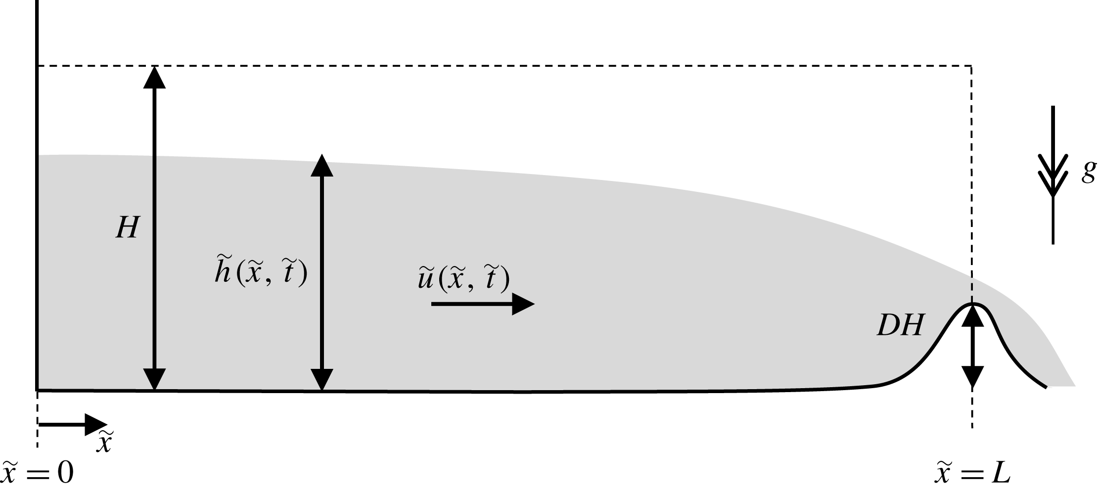
The configuration of the flow over a weir, showing the important dimensional variables. The vertical scale is exaggerated and the horizontal axis nonlinearly scaled to show the reservoir and the weir. The flow variables are decorated with a tilde to represent their dimensional form. The dimensionless variables are defined in § 2.

2 Formulation
In this contribution we model the unsteady, free draining of a horizontal reservoir of fluid over a confining barrier or through a constriction. The fluid in the reservoir is initially quiescent and its gravitationally driven motion arises following the partial removal of one of the end walls, allowing fluid to drain unsteadily (see figure 1 for a schematic of the configuration of the flow and important variables). In this investigation we neglect flow-induced mixing between the fluid initially in the reservoir and the surrounding fluid and thus our modelling framework applies to scenarios in which the fluids are effectively immiscible. We assume that the barrier and/or the constriction are localised to one end of the reservoir, so that away from this draining boundary the reservoir is of constant width and its base is at a constant elevation. The motion is also assumed to be shallow, so that the depth of the flowing layer is much smaller than the streamwise length scale, which implies that the velocity is predominantly parallel with the underlying boundary, vertical fluid accelerations are negligible and the pressure adopts a hydrostatic distribution. Thus in the bulk of the reservoir, away from the outflow boundary, the motion is unidirectional, and if viscous effects are negligible, dependent only on the streamwise coordinate and time; we may therefore adopt the shallow-water model for the fluid motion (Peregrine Reference Peregrine and Meyer1972).
The depth of the flowing layer is denoted by
 $h(x,t)$
and the maximum height of the barrier by
 $D$
; both are rendered dimensionless with respect to the initial depth of the reservoir,
 $H$
. The reservoir is of constant width,
 $W$
, apart from within the locality of the boundary across which the fluid drains; the minimum width of the channel relative to the uniform width is denoted by
 $w$
, and both the minimum width and maximum height occur at the same location. The horizontal flow velocity is denoted by
 $u(x,t)$
and it is made dimensionless with respect to
 $(\unicode[STIX]{x0394}\unicode[STIX]{x1D70C}gH/\unicode[STIX]{x1D70C})^{1/2}$
, where
 $\unicode[STIX]{x0394}\unicode[STIX]{x1D70C}$
is the density difference between the reservoir and ambient fluids and
 $\unicode[STIX]{x1D70C}$
is the density of the reservoir fluid. Both dependent variables are functions of
 $x$
and
 $t$
, the distance from the back wall of the reservoir and the time since initiation, respectively. The
 $x$
-axis is directed streamwise and is non-dimensionalised with respect to the reservoir length,
 $L$
. Finally time is made dimensionless with respect to
 $L/(\unicode[STIX]{x0394}\unicode[STIX]{x1D70C}gH/\unicode[STIX]{x1D70C})^{1/2}$
. The dimensionless governing equations, which express conservation of mass and the balance of streamwise momentum, are then given by
 $$\begin{eqnarray}\displaystyle & \displaystyle \frac{\unicode[STIX]{x2202}h}{\unicode[STIX]{x2202}t}+\frac{\unicode[STIX]{x2202}}{\unicode[STIX]{x2202}x}(uh)=0, & \displaystyle\end{eqnarray}$$
 $$\begin{eqnarray}\displaystyle & \displaystyle \frac{\unicode[STIX]{x2202}}{\unicode[STIX]{x2202}t}(uh)+\frac{\unicode[STIX]{x2202}}{\unicode[STIX]{x2202}x}\left(u^{2}h+\frac{1}{2}h^{2}\right)=0. & \displaystyle\end{eqnarray}$$
 $$\begin{eqnarray}u(0,t)=0.\end{eqnarray}$$
Fluid freely drains over the other boundary at which we enforce a mass- and energy-conserving condition that permits the relatively tranquil flow from the reservoir to be connected to the more rapid draining flow (Dake Reference Dake1983, § 4.3.4), given by
 $$\begin{eqnarray}u^{2}+2(h-D)-3\left(\frac{uh}{w}\right)^{2/3}=0,\quad \text{at }x=1.\end{eqnarray}$$
Details of the derivation of this boundary condition are given in appendix A. It is notable that by adopting the dimensionless velocity and time scales described above, neither the governing equations (2.1a
)–(2.1b
) nor the boundary conditions (2.2) and (2.3) feature the densities of the fluids. We further note that it is convenient to write (2.3) in terms of the Froude number at the boundary,
 $Fr=u(1,t)/\sqrt{h(1,t)}$
, in which case we find that
 $$\begin{eqnarray}Fr^{2}-3\left(\frac{Fr}{w}\right)^{2/3}=-2\left(1-\frac{D}{h}\right).\end{eqnarray}$$
Physically relevant solutions corresponds to
 $0\leqslant Fr\leqslant 1$
and we note that
 $Fr=1$
for
 $D=0$
and
 $w=1$
, recovering the standard condition for free-draining flow when in the absence of a barrier or constriction. This system of equations has been recently employed by Momen et al. (Reference Momen, Zheng, Bou-Zeid and Stone2017) to study unsteady gravity current drainage over an edge
 $(D=0,w=1)$
. We emphasise that the definition of this internal Froude number,
 $Fr$
, at the fixed position,
 $x=1$
is different from the Froude number introduced by Benjamin (Reference Benjamin1968), and more recently revisited by Ungarish & Hogg (Reference Ungarish and Hogg2018), which expresses the conditions at the front of a gravity current.
2.1 Hodograph variables
The shallow-water equations (2.1a
) and (2.1b
) are hyperbolic and may be written in terms of quantities
 $\unicode[STIX]{x1D6FC}=u+2h^{1/2}$
and
 $\unicode[STIX]{x1D6FD}=u-2h^{1/2}$
, which are invariant along characteristics (Whitham Reference Whitham1974). Thus we find that
 $$\begin{eqnarray}\frac{\text{d}\unicode[STIX]{x1D6FC}}{\text{d}t}=0\quad \text{on }\frac{\text{d}x}{\text{d}t}=u+h^{1/2}\quad \text{and}\quad \frac{\text{d}\unicode[STIX]{x1D6FD}}{\text{d}t}=0\quad \text{on }\frac{\text{d}x}{\text{d}t}=u-h^{1/2}.\end{eqnarray}$$
It is also possible to interchange the dependent and independent variables to treat
 $x$
and
 $t$
as functions of the characteristic invariants,
 $\unicode[STIX]{x1D6FC}$
and
 $\unicode[STIX]{x1D6FD}$
. This hodograph transformation converts the nonlinear governing equations into linear equations. In particular as shown by Hogg (Reference Hogg2006), the characteristic equations (2.5) are now given by
 $$\begin{eqnarray}\displaystyle & \displaystyle \frac{\unicode[STIX]{x2202}x}{\unicode[STIX]{x2202}\unicode[STIX]{x1D6FD}}=\frac{(3\unicode[STIX]{x1D6FC}+\unicode[STIX]{x1D6FD})}{4}\frac{\unicode[STIX]{x2202}t}{\unicode[STIX]{x2202}\unicode[STIX]{x1D6FD}}\quad \text{on }\unicode[STIX]{x1D6FC}=\text{const}., & \displaystyle\end{eqnarray}$$
 $$\begin{eqnarray}\displaystyle & \displaystyle \frac{\unicode[STIX]{x2202}x}{\unicode[STIX]{x2202}\unicode[STIX]{x1D6FC}}=\frac{(\unicode[STIX]{x1D6FC}+3\unicode[STIX]{x1D6FD})}{4}\frac{\unicode[STIX]{x2202}t}{\unicode[STIX]{x2202}\unicode[STIX]{x1D6FC}}\quad \text{on }\unicode[STIX]{x1D6FD}=\text{const}. & \displaystyle\end{eqnarray}$$
 $J=(\unicode[STIX]{x1D6FC}-\unicode[STIX]{x1D6FD})(\unicode[STIX]{x2202}t/\unicode[STIX]{x2202}\unicode[STIX]{x1D6FC})(\unicode[STIX]{x2202}t/\unicode[STIX]{x2202}\unicode[STIX]{x1D6FD})$
is finite and non-vanishing.
It is possible to find a fundamental solution to the adjoint governing equations and this Riemann solution can then aide the construction of the solution from conditions along the boundaries in the hodograph plane. This technique was used by Hogg and coworkers to solve some gravity current and hydraulic problems using quasi-analytical techniques (Antuono & Hogg Reference Antuono and Hogg2009; Antuono, Hogg & Brocchini Reference Antuono, Hogg and Brocchini2009; Goater & Hogg Reference Goater and Hogg2011; Hogg et al. Reference Hogg, Baldock and Pritchard2011). These analyses deploy the Riemann function, which is given by (Garabedian Reference Garabedian1986)
 $$\begin{eqnarray}B(a,b;\unicode[STIX]{x1D6FC},\unicode[STIX]{x1D6FD})=\frac{(a-b)^{3}}{(a-\unicode[STIX]{x1D6FD})^{3/2}(\unicode[STIX]{x1D6FC}-b)^{3/2}}{\mathcal{F}}\left[\frac{3}{2},\frac{3}{2};1;\frac{(a-\unicode[STIX]{x1D6FC})(\unicode[STIX]{x1D6FD}-b)}{(a-\unicode[STIX]{x1D6FD})(\unicode[STIX]{x1D6FC}-b)}\right],\end{eqnarray}$$
where
 ${\mathcal{F}}$
denotes a hypergeometric function. Integration around a closed curve,
 $\unicode[STIX]{x2202}{\mathcal{D}}$
, in the hodograph plane yields
 $$\begin{eqnarray}\int _{\unicode[STIX]{x2202}{\mathcal{D}}}\boldsymbol{f}\boldsymbol{\cdot }\text{d}\boldsymbol{x}=0,\end{eqnarray}$$
where
 $\boldsymbol{f}(a,b;\unicode[STIX]{x1D6FC},\unicode[STIX]{x1D6FD})=-V\hat{\boldsymbol{a}}+U\hat{\boldsymbol{b}}$
,
 $\text{d}\boldsymbol{x}=\text{d}a\hat{\boldsymbol{a}}+\text{d}b\hat{\boldsymbol{b}}$
and
 $$\begin{eqnarray}\displaystyle & \displaystyle U=-\frac{3}{2(a-b)}tB+\frac{B}{2}\frac{\unicode[STIX]{x2202}t}{\unicode[STIX]{x2202}b}-\frac{t}{2}\frac{\unicode[STIX]{x2202}B}{\unicode[STIX]{x2202}b}, & \displaystyle\end{eqnarray}$$
 $$\begin{eqnarray}\displaystyle & \displaystyle V=\frac{3}{2(a-b)}tB+\frac{B}{2}\frac{\unicode[STIX]{x2202}t}{\unicode[STIX]{x2202}a}-\frac{t}{2}\frac{\unicode[STIX]{x2202}B}{\unicode[STIX]{x2202}a}. & \displaystyle\end{eqnarray}$$
Thus
 $a$
and
 $b$
are dummy variables for the evaluation of integral (2.8) around the closed path
 $\unicode[STIX]{x2202}{\mathcal{D}}$
in the hodograph plane.
The method of characteristics and the hodograph transformation will be used to construct the solution for this free-draining flow and will be shown to bring considerable insight to the ensuing dynamics, elucidating the nonlinear wave reflections from the back wall
 $(x=0)$
and the barrier or constriction
 $(x=1)$
. Throughout this paper we will use the following terminology: complex wave region refers to a domain within which both characteristic variables are varying; simple wave region refers to a domain within which one of the characteristic variables is constant and the other varying; and uniform region refers to a domain within which both characteristic variables are constant.
2.2 Numerical method
We also integrate the governing equations (2.1a
) and (2.1b
) numerically. This is done utilising a central-upwind scheme (Kurganov et al.
Reference Kurganov, Noelle and Petrova2001) with a minmod piecewise linear reconstruction (see Kurganov et al.
Reference Kurganov, Noelle and Petrova2001 equation (3.16) with
 $\unicode[STIX]{x1D703}=1$
). The resultant semi-discrete system is then time stepped using a third-order Runge–Kutta scheme composed of multiple Euler time steps (Shu & Osher Reference Shu and Osher1988). This scheme is positivity preserving, i.e. we always have
 $h\geqslant 0$
, due to the Courant–Friedrichs–Lewy (CFL) condition and lack of source terms.
To impose boundary conditions we use three ghost cells at each domain end, for which we must find values consistent with both the governing equations and the boundary conditions. We discuss below the process of finding values at the domain end itself, but to impose values in the ghost cells some extrapolation utilising the domain endpoint values and interior values is required. Zeroth-order extrapolation is inconsistent with the first-order reconstruction in the cells, and first-order extrapolation can produce negative depths. To resolve this issue we consider the ghost cells to have size
 $\unicode[STIX]{x1D716}\unicode[STIX]{x0394}x$
(where
 $\unicode[STIX]{x0394}x$
is the cell size in the interior) and limit
 $\unicode[STIX]{x1D716}\rightarrow 0$
. Under this limit all consistent extrapolation procedures converge to enforce the values of
 $h$
and
 $uh$
at the domain end across all ghost cells.
To deduce how the domain endpoint values should be evolved we consider the general form of a homogeneous system of
 $m$
hyperbolic partial differential equations of a variable
 $Q(x,t)\in \mathbb{R}^{m}$
 $$\begin{eqnarray}\frac{\unicode[STIX]{x2202}Q}{\unicode[STIX]{x2202}t}+A(Q,x,t)\frac{\unicode[STIX]{x2202}Q}{\unicode[STIX]{x2202}x}=\unicode[STIX]{x1D6F9}(Q,x,t).\end{eqnarray}$$
For the purposes of imposing boundary conditions alone, (2.11) is adjusted by including a small amount of diffusion
 $0<{\mathcal{D}}\ll 1$
, and then multiplying by the
 $p$
th left eigenvector of
 $A(Q,x,t)$
,
 $l^{p}(Q,x,t)$
corresponding to eigenvalue
 $\unicode[STIX]{x1D706}^{p}(Q,x,t)$
, which results in the characteristic form
 $$\begin{eqnarray}l^{p}\frac{\unicode[STIX]{x2202}Q}{\unicode[STIX]{x2202}t}+\unicode[STIX]{x1D706}^{p}l^{p}\frac{\unicode[STIX]{x2202}Q}{\unicode[STIX]{x2202}x}={\mathcal{D}}l^{p}\frac{\unicode[STIX]{x2202}^{2}Q}{\unicode[STIX]{x2202}x^{2}}+l^{p}\unicode[STIX]{x1D6F9}.\end{eqnarray}$$
Diffusion is required for cases when a weak solution to the system contains a discontinuity between the bulk and the boundary, that is when the value at the boundary is not the limit of the interior values. Such a situation is not permitted in the vanishing viscosity solution, and to ensure this solution is found we include a small amount of diffusion. The boundary conditions are of the form
 $f(Q,t)=0$
, where the function
 $f:\mathbb{R}^{m}\times \mathbb{R}\rightarrow \mathbb{R}^{k}$
, and specify the values advected by characteristics entering the domain. We focus our discussion on the right-hand end of the domain, that is we are at
 $x=x_{e}$
such that the domain is
 $x<x_{e}$
(and in this study
 $x_{e}=1$
). This means that we must enforce (2.12) for those
 $p$
such that
 $\unicode[STIX]{x1D706}^{p}\geqslant 0$
as well as the boundary conditions to determine
 $Q_{e}(t)=Q(x_{e},t)$
. We discretise the
 $x$
derivatives using finite differences over the grid with cell size,
 $\unicode[STIX]{x0394}x$
, and take
 ${\mathcal{D}}=\max _{p}|\unicode[STIX]{x1D706}^{p}|\unicode[STIX]{x0394}x$
which is of the same form as the effective diffusion from the method in the bulk and is stable under the same CFL condition. This yields a system of differential algebraic equations (DAE) (see Ascher & Petzold Reference Ascher and Petzold1998; Kunkel & Mehrmann Reference Kunkel and Mehrmann2006) of the form
 $$\begin{eqnarray}\displaystyle & \displaystyle L(Q_{e},t)\frac{\text{d}Q_{e}}{\text{d}t}=C(Q_{e},t), & \displaystyle\end{eqnarray}$$
 $$\begin{eqnarray}\displaystyle & \displaystyle f(Q_{e},t)=0, & \displaystyle\end{eqnarray}$$
 $L$
are the
 $m-k$
left eigenvectors with
 $\unicode[STIX]{x1D706}^{p}\geqslant 0$
, and we treat the values of the internal cells as known functions of
 $t$
so that their values do not appear in the arguments of
 $C$
. For the shallow-water equations and boundary conditions given by (2.1a
), (2.1b
), (2.2) and (2.3), we note that
 $m=2$
and
 $k=1$
; thus at both boundaries, the rear wall
 $(x=0)$
and the barrier
 $(x=1)$
, there is one outward propagating characteristic and one boundary condition to be applied. We denote the discrete times by
 $t^{n}$
, the values at these discrete times
 $Q_{e}^{n}=Q_{e}(t^{n})$
, and the difference over a time step of size
 $\unicode[STIX]{x0394}t$
by
 $\unicode[STIX]{x0394}Q_{e}^{n}=Q_{e}^{n+1}-Q_{e}^{n}$
. To be consistent with the time stepping of the ordinary differential equation (ODE) portion of the DAE (2.13a
) is discretised using Euler’s method, and for the algebraic portion (2.13b
) we enforce
 $f=0$
at time
 $t^{n+1}$
using a single step of the Newton–Raphson method with initial guess of the difference
 $\unicode[STIX]{x0394}Q_{e}^{n,0}$
. This results in the explicit scheme
 $$\begin{eqnarray}\left[\begin{array}{@{}c@{}}L(Q_{e}^{n},t^{n})\\ F(Q_{e}^{n}+\unicode[STIX]{x0394}Q_{e}^{n,0},t^{n+1})\end{array}\right]\unicode[STIX]{x0394}Q_{e}^{n}=\left[\begin{array}{@{}c@{}}C(Q_{e}^{n},t^{n})\unicode[STIX]{x0394}t\\ F(Q_{e}^{n}+\unicode[STIX]{x0394}Q_{e}^{n,0},t^{n+1})\unicode[STIX]{x0394}Q_{e}^{n,0}-f(Q_{e}^{n}+\unicode[STIX]{x0394}Q_{e}^{n,0},t^{n+1})\end{array}\right]\!,\qquad\end{eqnarray}$$
where
 $F=\unicode[STIX]{x2202}f/\unicode[STIX]{x2202}Q$
and is non-vanishing, which is similar to the poststabilisation method with one iteration of projection (Ascher & Petzold Reference Ascher and Petzold1998, § 10.2).
As we are solving an ODE on a manifold (2.13) using Euler’s method, we can show the problem under consideration has sufficient smoothness conditions so that the method has a truncation error of
 $O(\unicode[STIX]{x0394}t)$
. Similarly, if
 $\overline{\unicode[STIX]{x0394}Q_{e}}^{n}$
is the limit of iterating (2.14) with the output
 $\unicode[STIX]{x0394}Q^{n}$
being taken as the next input
 $\unicode[STIX]{x0394}Q_{e}^{n,0}$
(the implicit version of (2.14)), then we can show that the Newton–Raphson portion of our method will provide
 $f(Q^{n+1},t^{n+1})=O(\Vert \overline{\unicode[STIX]{x0394}Q_{e}}^{n}-\unicode[STIX]{x0394}Q_{e}^{n,0}\Vert ^{2})$
and then if
 $\Vert \overline{\unicode[STIX]{x0394}Q_{e}}^{n}-\unicode[STIX]{x0394}Q_{e}^{n,0}\Vert =O(\unicode[STIX]{x0394}t)$
, we deduce that the convergence to the manifold is second order. Finally we can use the fact that, as time evolves, we are repeatedly performing Newton–Raphson steps on very similar problems to improve the scheme further. By taking our guess to be the value of a recent time step, for example
 $\unicode[STIX]{x0394}Q_{e}^{n,0}=\unicode[STIX]{x0394}Q_{e}^{n-1}$
, then
 $f(Q^{n+1},t^{n+1})=O(\unicode[STIX]{x0394}t^{4})$
and the scheme provides fourth order convergence to the manifold.
To use this method with the Runge–Kutta time steps from Shu & Osher (Reference Shu and Osher1988) some modifications must be made. These time steps are composed of multiple Euler time steps, which we shall denote by the operator
 $E$
, and the intermediate results by
 $Q_{e}^{(i)}$
where
 $Q_{e}^{(0)}=Q_{e}^{n}$
. The intermediate results are from computations of the form
 $$\begin{eqnarray}Q_{e}^{(i+1)}=\unicode[STIX]{x1D702}_{i}Q_{e}^{(0)}+(1-\unicode[STIX]{x1D702}_{i})E(Q_{e}^{(i)}),\end{eqnarray}$$
where
 $0\leqslant \unicode[STIX]{x1D702}_{i}\leqslant 1$
. Based on the results presented in Kunkel & Mehrmann (Reference Kunkel and Mehrmann2006, § 5.2) we argue that it is appropriate to approximately enforce
 $f(Q_{e}^{(i+1)},t^{(i+1)})=0$
, where
 $t^{(i)}$
is the time at which
 $Q_{e}^{(i)}$
is an approximation, rather than
 $f(E(Q_{e}^{(i)}),t^{(i)}+\unicode[STIX]{x0394}t)=0$
as in (2.13). We therefore use a modified version of our scheme suitable for the application of (2.15), specifically
 $$\begin{eqnarray}\left[\begin{array}{@{}c@{}}L(Q_{e}^{(i)},t^{(i)})\\ (1-\unicode[STIX]{x1D702}_{i})F(Q_{e}^{(i)\star },t^{(i+1)})\end{array}\right]\unicode[STIX]{x0394}Q_{e}^{(i)}=\left[\begin{array}{@{}c@{}}C(Q_{e}^{(i)},t^{(i)})\unicode[STIX]{x0394}t\\ (1-\unicode[STIX]{x1D702}_{i})F(Q_{e}^{(i)\star },t^{(i+1)})\unicode[STIX]{x0394}Q_{e}^{(i),0}-f(Q_{e}^{(i)\star },t^{(i+1)})\end{array}\right]\!,\qquad\end{eqnarray}$$
where
 $$\begin{eqnarray}Q_{e}^{(i)\star }=\unicode[STIX]{x1D702}_{i}Q_{e}^{(0)}+(1-\unicode[STIX]{x1D702}_{i})(Q_{e}^{(i)}+\unicode[STIX]{x0394}Q_{e}^{(i),0}),\end{eqnarray}$$
and
 $E(Q_{e}^{(i)})=Q_{e}^{(i)}+\unicode[STIX]{x0394}Q^{(i)}$
. The initial guesses are taken as
 $\unicode[STIX]{x0394}Q_{e}^{(i),0}=\unicode[STIX]{x0394}Q_{e}^{(0)}$
, except for when
 $i=0$
in which case
 $\unicode[STIX]{x0394}Q_{e}^{(0),0}=\unicode[STIX]{x0394}Q_{e}^{n-1}$
.
The numerical scheme has been validated against a variety of known solutions, but for the purposes of this paper we simply observe the excellent correspondence between the simulations and analytic solutions at early times (see §§ 3.2 and 3.3), and the convergence to the asymptotic wave structure at late times, for the particular problem considered here.
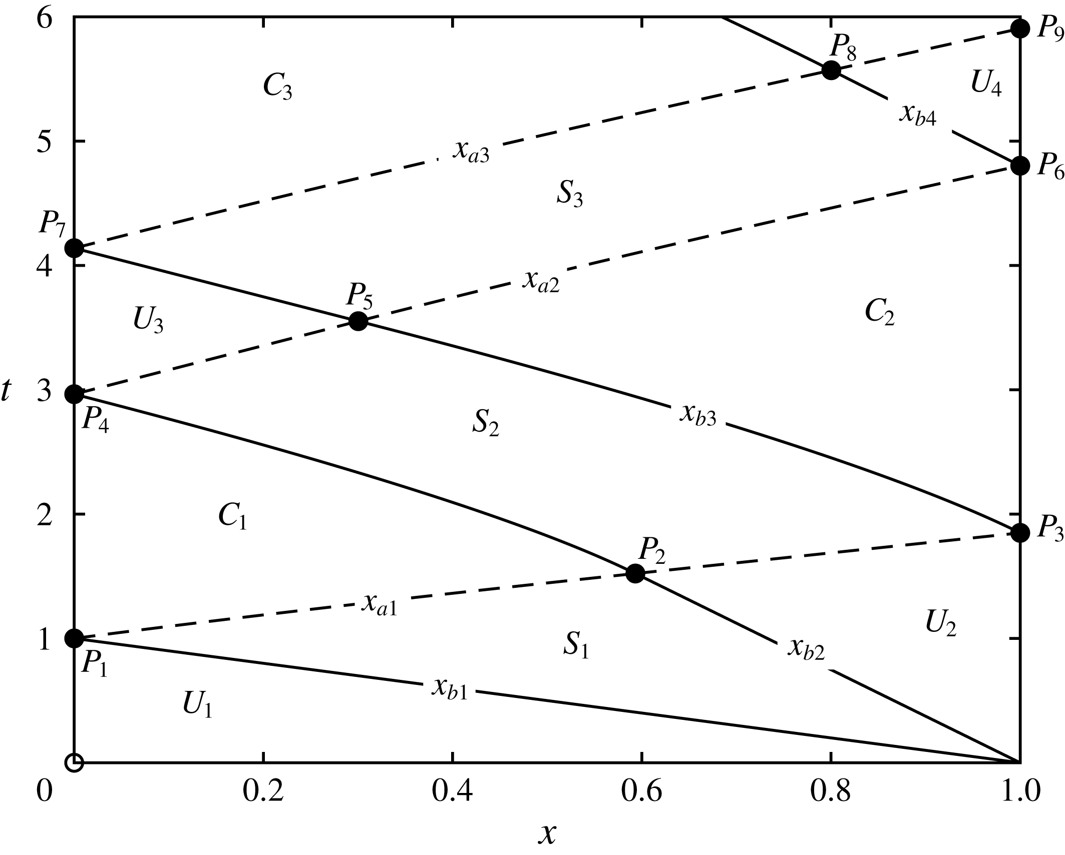
The characteristic plane for the unsteady draining of fluid from a partially confined reservoir with barrier height,
 $D=0.05$
and width
 $w=1$
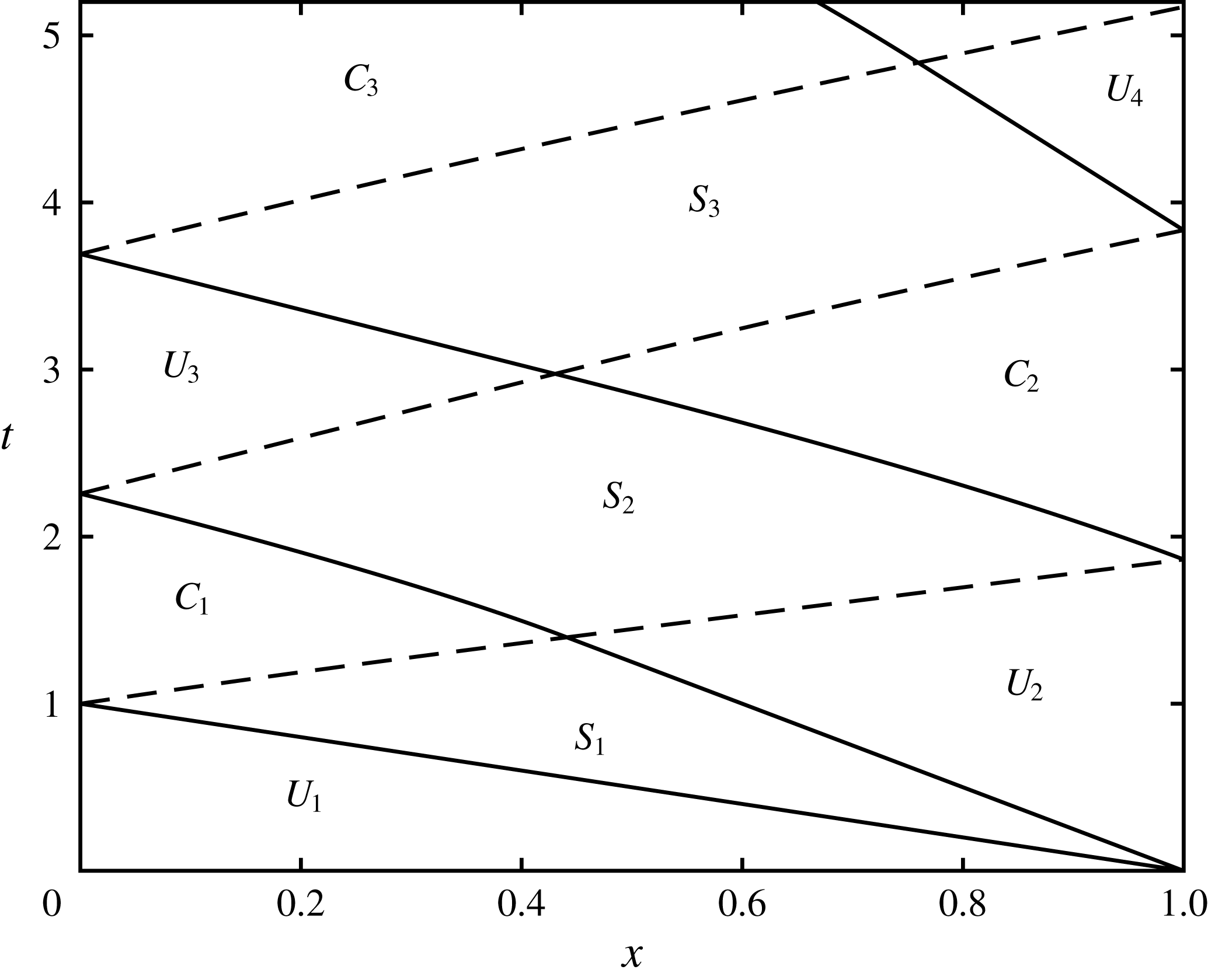
. In this figure we plot and label the uniform, simple and complex wave regions following the initiation of the flow. We also plot the characteristics bounding the wave regions; the suffices
 $a$
and
 $b$
denote the
 $\unicode[STIX]{x1D6FC}$
- and
 $\unicode[STIX]{x1D6FD}$
-characteristics and are plotted with dashed and solid lines, respectively. (These characteristic curves are defined in § 3.) Additionally we label key points in the characteristic plane, which occur at the boundaries of the wave regions.

The hodograph plane for the unsteady draining of fluid from a partially confined reservoir, with barrier height,
 $D=0.05$
and
 $w=1$
. In this figure, the solid line corresponds to the free-draining boundary at
 $x=1$
and the dotted line to the impermeable boundary at
 $x=0$
. Uniform regions are depicted by points in the hodograph planes and are labelled
 $U_{i}$
 $(i=1-4)$
, while simple wave regions correspond to dashed straight line segments aligned with the axes and are labelled
 $S_{i}$
 $(i=1-3)$
. Finally, complex wave regions are labelled
 $C_{i}\,(i=1-3)$
. This figure shows the wave pattern that emerges following flow initiation and the first three reflections from the end wall and free-draining boundary. This pattern of successive reflections will continue indefinitely, approaching the end state in which the fluid is quiescent and of depth equal to the barrier height; this is where the two boundary curves intersect at
 $\unicode[STIX]{x1D6FC}=-\unicode[STIX]{x1D6FD}=2\sqrt{D}$
.

3 Draining over a weir
In this section we analyse the unsteady drainage of a reservoir from lock-release initial conditions over a weir of dimensionless height
 $D$
and width
 $w$
. We use the method of characteristics and hodograph techniques to construct the motion during the initial phases (§§ 3.1 and 3.2), while the motion at late times is found asymptotically (§ 3.3). We also present results from the direct numerical integration of the governing equations.
3.1 Initial motion:
 $t\leqslant 1$

The drainage condition (2.3) yields Froude numbers in the range
 $0\leqslant Fr<1$
(provided
 $D>0$
) and so at that boundary
 $(x=1)$
there is one outflowing characteristic direction and one inflowing. This means that it is straightforward to construct the initial solution (valid for
 $t\leqslant 1$
) since the characteristic variable
 $\unicode[STIX]{x1D6FC}$
is determined by the initial conditions. Thus throughout the portion of the domain associated with the initial conditions, we find that
 $\unicode[STIX]{x1D6FC}=2$
and within this portion there is a rarefaction centred on
 $x=1$
, which we term simple wave region
 $S_{1}$
. Within
 $S_{1}$
,
 $-2\leqslant \unicode[STIX]{x1D6FD}\leqslant \unicode[STIX]{x1D6FD}_{\ast }$
, where
 $\unicode[STIX]{x1D6FD}_{\ast }$
is a function of
 $D$
and
 $w$
and is the maximum value of
 $\unicode[STIX]{x1D6FD}$
in this region, determined from (2.3) with
 $\unicode[STIX]{x1D6FC}=2$
. (Since
 $0\leqslant Fr<1$
, we can show that
 $-2\leqslant \unicode[STIX]{x1D6FD}_{\ast }<-2/3$
.) The solution for the velocity and height fields within
 $S_{1}$
are given by
 $$\begin{eqnarray}u=\frac{2}{3}\left(1+\frac{(x-1)}{t}\right)\quad \text{and}\quad h=\frac{1}{9}\left(2-\frac{(x-1)}{t}\right)^{2},\end{eqnarray}$$
for
 $x_{b1}\equiv 1-t<x<x_{b2}\equiv 1+(2+3\unicode[STIX]{x1D6FD}_{\ast })t/4$
(see figure 2). Upstream of this rarefaction, the fluid remains undisturbed from its initial state with
 $h=1$
and
 $u=0$
; we denoted this uniform region as
 $U_{1}$
. Downstream of the rarefaction, there is a uniform region attached to the right boundary
 $(x=1)$
, within which
 $u=1+\unicode[STIX]{x1D6FD}_{\ast }/2$
and
 $h=(2-\unicode[STIX]{x1D6FD}_{\ast })^{2}/16$
; we denote this as region
 $U_{2}$
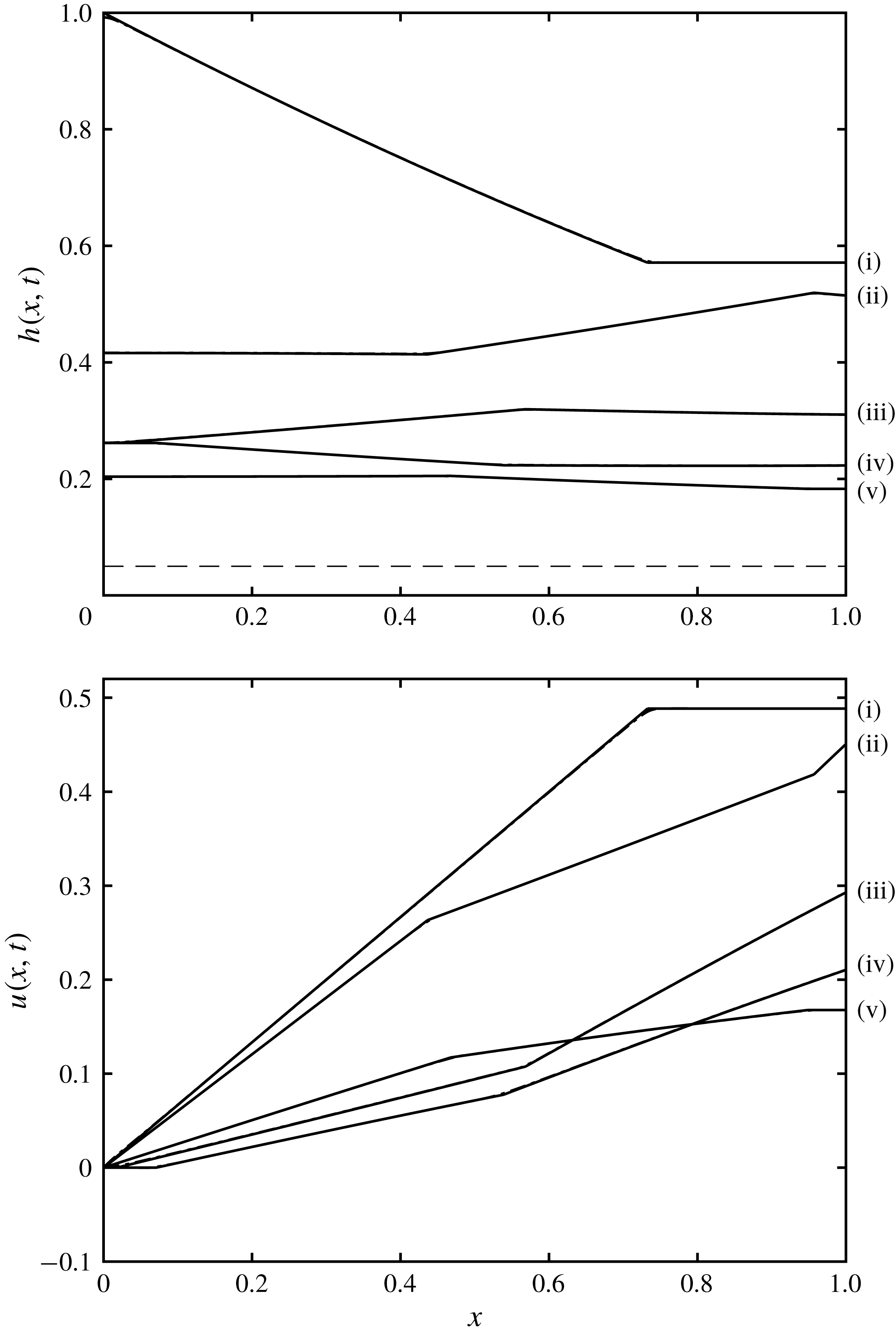
. Example profiles of height and velocity are plotted in figure 5. We observe that the fluid slumps gravitationally, progressively mobilising fluid within the reservoir and that its motion is ‘choked’ by draining at the outflow. These solutions for the flow are valid until the rearward propagating characteristic reaches the back wall of the reservoir, which occurs at
 $t=1$
. Thereafter there are reflections from this wall and the motion becomes more complicated.
3.2 Motion for
$t\geqslant 1$

When
 $t\geqslant 1$
, the structure of the solution for the height and velocity fields is altered due to reflection first from the back wall of the reservoir and then from the free-draining boundary at the front. It is useful to treat this dynamics in the characteristic plane (figure 2) and in the hodograph plane (figure 3), both of which reveal the successive wave reflections. As described above, the initial phase of the motion involves a simple wave region,
 $S_{1}$
, sandwiched between two uniform regions,
 $U_{1}$
and
 $U_{2}$
, which are attached to the boundaries of the reservoir. In the hodograph plane, a simple wave region corresponds to a line segment parallel to the coordinate axes and
 $S_{1}$
is given by
 $\unicode[STIX]{x1D6FC}=2$
and
 $-2\leqslant \unicode[STIX]{x1D6FD}\leqslant \unicode[STIX]{x1D6FD}_{\ast }$
. Uniform regions correspond to points in the hodograph plane;
 $U_{1}$
is given by
 $(\unicode[STIX]{x1D6FC},\unicode[STIX]{x1D6FD})=(2,-2)$
and
 $U_{2}$
by
 $(\unicode[STIX]{x1D6FC},\unicode[STIX]{x1D6FD})=(2,\unicode[STIX]{x1D6FD}_{\ast })$
. Complex wave regions correspond to connected domains in the hodograph plane (see figure 3).
The reflection from the back wall generates a complex wave region
 $C_{1}$
, which is bounded by the characteristic curve on which
 $\unicode[STIX]{x1D6FC}=2$
. We denote that curve parametrically by
 $x_{a1}(\unicode[STIX]{x1D6FD})$
and
 $t_{a1}(\unicode[STIX]{x1D6FD})$
and it is straightforward to show that
 $$\begin{eqnarray}t_{a1}=\frac{8}{(2-\unicode[STIX]{x1D6FD})^{3/2}}\quad \text{and}\quad x_{a1}=1+\frac{2(2+3\unicode[STIX]{x1D6FD})}{(2-\unicode[STIX]{x1D6FD})^{3/2}}.\end{eqnarray}$$
The region,
 $C_{1}$
, is also bounded by the characteristic on which
 $\unicode[STIX]{x1D6FD}=\unicode[STIX]{x1D6FD}_{\ast }$
, denoted by
 $x_{b2}(t)$
, which occurs at the leading edge of the rarefaction fan in the simple wave region,
 $S_{1}$
(see figure 2). It is given from (3.1) by
 $x_{b2}=1+(2+3\unicode[STIX]{x1D6FD}_{\ast })t/4$
. The curve
 $x_{a1}$
intersects
 $x_{b2}$
at the point
 $P_{2}$
with coordinates,
 $(x,t)=(1+2(2+3\unicode[STIX]{x1D6FD}_{\ast })/(2-\unicode[STIX]{x1D6FD}_{\ast })^{3/2},8/(2-\unicode[STIX]{x1D6FD}_{\ast })^{3/2})$
. Thereafter
 $x_{a1}$
follows a straight line that bounds the uniform region,
 $U_{2}$
until reaching the outflow at
 $x=1$
. In this portion the characteristics are given by
 $$\begin{eqnarray}\frac{x-x_{a1}(\unicode[STIX]{x1D6FD}_{\ast })}{t-t_{a1}(\unicode[STIX]{x1D6FD}_{\ast })}=\frac{6+\unicode[STIX]{x1D6FD}_{\ast }}{4},\end{eqnarray}$$
and the point,
 $P_{3}$
, at the outflow is
 $(1,16/[(6+\unicode[STIX]{x1D6FD}_{\ast })(2-\unicode[STIX]{x1D6FD}_{\ast })^{1/2}])$
. The complex wave region,
 $C_{1}$
, may be calculated using the Riemann function, integrated around a trajectory in the hodograph plane, as demonstrated by Hogg (Reference Hogg2006); it is compactly given by
 $$\begin{eqnarray}t(\unicode[STIX]{x1D6FC},\unicode[STIX]{x1D6FD})=B(2,-2;\unicode[STIX]{x1D6FC},\unicode[STIX]{x1D6FD}),\end{eqnarray}$$
and the solution for
 $x$
is given by integrating along
 $\unicode[STIX]{x1D6FC}$
-characteristics from the back wall, using (2.6a
) to show
 $$\begin{eqnarray}x(\unicode[STIX]{x1D6FC},\unicode[STIX]{x1D6FD})=\frac{(3\unicode[STIX]{x1D6FC}+\unicode[STIX]{x1D6FD})}{4}t(\unicode[STIX]{x1D6FC},\unicode[STIX]{x1D6FD})-\frac{\unicode[STIX]{x1D6FC}}{2}t(\unicode[STIX]{x1D6FC},-\unicode[STIX]{x1D6FC})-\frac{1}{4}\int _{-\unicode[STIX]{x1D6FC}}^{\unicode[STIX]{x1D6FD}}t(\unicode[STIX]{x1D6FC},b)\,\text{d}b.\end{eqnarray}$$
In the characteristic plane, the continuation of the
 $\unicode[STIX]{x1D6FD}=\unicode[STIX]{x1D6FD}_{\ast }$
characteristic beyond
 $P_{2}$
bounds the region
 $C_{1}$
(see figure 2). It meets the back wall at
 $P_{4}=(0,t_{b2}(-\unicode[STIX]{x1D6FD}_{\ast }))$
, where
 $$\begin{eqnarray}t_{b2}(\unicode[STIX]{x1D6FC})=B(2,-2;\unicode[STIX]{x1D6FC},-\unicode[STIX]{x1D6FD}_{\ast }).\end{eqnarray}$$
The
 $\unicode[STIX]{x1D6FD}$
-characteristics starting from the uniform region,
 $U_{2}$
generate the simple wave region,
 $S_{2}$
, within which
 $-\unicode[STIX]{x1D6FD}_{\ast }\leqslant \unicode[STIX]{x1D6FC}\leqslant 2$
(see figures 2 and 3). The trajectory of the characteristic from point
 $P_{3}$
on which
 $\unicode[STIX]{x1D6FD}=\unicode[STIX]{x1D6FD}_{\ast }$
is denoted by
 $(x_{b3},t_{b3})$
and satisfies
 $$\begin{eqnarray}\frac{\unicode[STIX]{x2202}x_{b3}}{\unicode[STIX]{x2202}\unicode[STIX]{x1D6FC}}=\frac{(\unicode[STIX]{x1D6FC}+3\unicode[STIX]{x1D6FD}_{\ast })}{4}\frac{\unicode[STIX]{x2202}t_{b3}}{\unicode[STIX]{x2202}\unicode[STIX]{x1D6FC}}.\end{eqnarray}$$
However on
 $\unicode[STIX]{x1D6FC}$
-characteristics within
 $S_{2}$
, we also find that
 $$\begin{eqnarray}\frac{x-x_{b2}}{t-t_{b2}}=\frac{3\unicode[STIX]{x1D6FC}+\unicode[STIX]{x1D6FD}_{\ast }}{4}.\end{eqnarray}$$
Thus we may establish
 $$\begin{eqnarray}t_{b3}-t_{b2}=\frac{-8(2+3\unicode[STIX]{x1D6FD}_{\ast })}{(6+\unicode[STIX]{x1D6FD}_{\ast })(\unicode[STIX]{x1D6FC}-\unicode[STIX]{x1D6FD}_{\ast })^{3/2}},\end{eqnarray}$$
and then
 $x_{b3}-x_{b2}$
may be deduced from (3.8). This
 $\unicode[STIX]{x1D6FD}$
-characteristic,
 $(x_{b3},t_{b3})$
, forms one of the boundaries to the complex wave region at the front,
 $C_{2}$
, and to the uniform region,
 $U_{3}$
, adjacent to the back wall. In particular the point
 $P_{5}$
is determined by the first location along this characteristic on which the velocity vanishes, which is given by
 $\unicode[STIX]{x1D6FC}=-\unicode[STIX]{x1D6FD}=-\unicode[STIX]{x1D6FD}_{\ast }$
. Beyond
 $P_{5}$
, the
 $\unicode[STIX]{x1D6FD}$
-characteristic is a straight line given by
 $$\begin{eqnarray}\frac{x-x_{b3}(-\unicode[STIX]{x1D6FD}_{\ast })}{t-t_{b3}(-\unicode[STIX]{x1D6FD}_{\ast })}=-\frac{\unicode[STIX]{x1D6FD}_{\ast }}{2}.\end{eqnarray}$$
This straight segment intersects the back wall at point
 $P_{7}= (\!0,t_{b3}(-\unicode[STIX]{x1D6FD}_{\ast })+2x_{b3}$
 $(-\unicode[STIX]{x1D6FD}_{\ast })/\unicode[STIX]{x1D6FD}_{\ast }\!)$
.
Constructing the solution within the complex wave region,
 $C_{2}$
entails the use of the Riemann function (2.7) and the conversion of the boundary conditions into hodograph variables. In particular the free-draining condition, given by (2.3), may be written as
 $$\begin{eqnarray}\frac{\text{d}x}{\text{d}\unicode[STIX]{x1D6FC}}=0\quad \text{on }\unicode[STIX]{x1D6FD}=\unicode[STIX]{x1D6FD}_{s}(\unicode[STIX]{x1D6FC}),\end{eqnarray}$$
We note that given a barrier height,
 $D$
, that
 $\unicode[STIX]{x1D6FD}_{s}(\unicode[STIX]{x1D6FC})$
determines a curve in the hodograph plane such that
 $\unicode[STIX]{x1D6FD}_{s}(2)=\unicode[STIX]{x1D6FD}_{\ast }$
and that
 $\unicode[STIX]{x1D6FD}(2\sqrt{D})=-2\sqrt{D}$
, the latter condition corresponding to no flow when the fluid depth matches the height of the barrier. (This function,
 $\unicode[STIX]{x1D6FD}_{s}(\unicode[STIX]{x1D6FC})$
, is plotted as a solid curve in figure 3 for
 $D=0.05$
.) From (2.3), we also find that
 $$\begin{eqnarray}\frac{\text{d}\unicode[STIX]{x1D6FD}_{s}}{\text{d}\unicode[STIX]{x1D6FC}}=\frac{(Fr^{4/3}-1/w^{2/3})(Fr-2)-2DFr^{1/3}/h}{(Fr^{4/3}-1/w^{2/3})(Fr+2)-2DFr^{1/3}/h},\end{eqnarray}$$
and this implies that
 $\text{d}\unicode[STIX]{x1D6FD}_{s}/\text{d}\unicode[STIX]{x1D6FC}=-1$
when
 $Fr=0$
. Thus the curve
 $\unicode[STIX]{x1D6FD}_{s}$
approaches its end point at
 $\unicode[STIX]{x1D6FD}_{s}=-2\sqrt{D}$
tangentially to the line
 $\unicode[STIX]{x1D6FD}=-\unicode[STIX]{x1D6FC}$
(see figure 3). (The case without a barrier is different: when
 $D=0$
, the outflow Froude number,
 $Fr$
, does not vary with the flow depth,
 $h$
and so the boundary curve,
 $\unicode[STIX]{x1D6FD}_{s}$
, is a straight line of gradient
 $\text{d}\unicode[STIX]{x1D6FD}_{s}/\text{d}\unicode[STIX]{x1D6FC}=(Fr-2)/(Fr+2)$
.) Using the characteristic equations (2.6a
) and (2.6b
), we can show that the boundary condition (3.11) is given by
 $$\begin{eqnarray}2(\unicode[STIX]{x1D6FC}+\unicode[STIX]{x1D6FD}_{s})\left(\frac{\unicode[STIX]{x2202}t}{\unicode[STIX]{x2202}\unicode[STIX]{x1D6FC}}+\frac{\text{d}\unicode[STIX]{x1D6FD}_{s}}{\text{d}\unicode[STIX]{x1D6FC}}\frac{\unicode[STIX]{x2202}t}{\unicode[STIX]{x2202}\unicode[STIX]{x1D6FD}}\right)+(\unicode[STIX]{x1D6FD}_{s}-\unicode[STIX]{x1D6FC})\left(\frac{\unicode[STIX]{x2202}t}{\unicode[STIX]{x2202}\unicode[STIX]{x1D6FC}}-\frac{\text{d}\unicode[STIX]{x1D6FD}_{s}}{\text{d}\unicode[STIX]{x1D6FC}}\frac{\unicode[STIX]{x2202}t}{\unicode[STIX]{x2202}\unicode[STIX]{x1D6FD}}\right)=0\quad \text{on }\unicode[STIX]{x1D6FD}=\unicode[STIX]{x1D6FD}_{s}(\unicode[STIX]{x1D6FC}).\end{eqnarray}$$
The other perimeter data in the hodograph plane are supplied by
 $t=t_{b3}(\unicode[STIX]{x1D6FC})$
along
 $\unicode[STIX]{x1D6FD}=\unicode[STIX]{x1D6FD}_{\ast }$
. We then integrate around the closed curve
 $OQRT$
, as depicted in figure 4. The coordinates of these points in the hodograph plane are
 $O$
,
 $(2,\unicode[STIX]{x1D6FD}_{\ast })$
;
 $Q$
,
 $(\unicode[STIX]{x1D6FC},\unicode[STIX]{x1D6FD}_{\ast })$
;
 $R$
,
 $(\unicode[STIX]{x1D6FC},\unicode[STIX]{x1D6FD}_{s})$
; and
 $T$
,
 $(\unicode[STIX]{x1D6FC}_{s},\unicode[STIX]{x1D6FD}_{s})$
. The curves
 $OQ$
,
 $QR$
and
 $RT$
correspond to straight line segments in the hodograph plane aligned with one of the coordinate axes, and the curve
 $RT$
corresponds to the free-draining boundary condition (
 $\unicode[STIX]{x1D6FC}=\unicode[STIX]{x1D6FC}_{s}$
and
 $\unicode[STIX]{x1D6FD}=\unicode[STIX]{x1D6FD}_{s}$
). Integration of (2.8) around
 $OQRT$
yields
 $$\begin{eqnarray}\displaystyle & & \displaystyle t(\unicode[STIX]{x1D6FC},\unicode[STIX]{x1D6FD}_{s})=B(\unicode[STIX]{x1D6FC},\unicode[STIX]{x1D6FD}_{\ast };\unicode[STIX]{x1D6FC},\unicode[STIX]{x1D6FD}_{s})t_{b3}(\unicode[STIX]{x1D6FC})+B(2,\unicode[STIX]{x1D6FD}_{\ast };\unicode[STIX]{x1D6FC},\unicode[STIX]{x1D6FD}_{s})t_{b3}(2)\left(\frac{2+\unicode[STIX]{x1D6FD}_{\ast }}{2-\unicode[STIX]{x1D6FD}_{\ast }}-\frac{1}{2}\right)\nonumber\\ \displaystyle & & \displaystyle \quad +\,B(\unicode[STIX]{x1D6FC}_{s},\unicode[STIX]{x1D6FD}_{s};\unicode[STIX]{x1D6FC},\unicode[STIX]{x1D6FD}_{s})t(\unicode[STIX]{x1D6FC}_{s},\unicode[STIX]{x1D6FD}_{s})\left(\frac{1}{2}-\frac{(\unicode[STIX]{x1D6FC}_{s}+\unicode[STIX]{x1D6FD}_{s})}{\unicode[STIX]{x1D6FC}_{s}-\unicode[STIX]{x1D6FD}_{s}}\right)-\int _{2}^{\unicode[STIX]{x1D6FC}}\left(\frac{\unicode[STIX]{x2202}B}{\unicode[STIX]{x2202}a}-\frac{3B}{2(a-\unicode[STIX]{x1D6FD}_{\ast })}\right)t_{b3}(a)\,\text{d}a\nonumber\\ \displaystyle & & \displaystyle \quad -\,\int _{\unicode[STIX]{x1D6FC}_{s}}^{2}\frac{t(a_{s},b_{s})}{2(a_{s}-b_{s})}\left((3a_{s}+b_{s})\left(\frac{\unicode[STIX]{x2202}B}{\unicode[STIX]{x2202}a}-\frac{B}{a_{s}-b_{s}}\right)\right.\nonumber\\ \displaystyle & & \displaystyle \quad +\left.(a_{s}+3b_{s})\frac{\text{d}b_{s}}{\text{d}a}\left(\frac{\unicode[STIX]{x2202}B}{\unicode[STIX]{x2202}b}+\frac{B}{a_{s}-b_{s}}\right)\right)\,\text{d}a.\end{eqnarray}$$
In the first integral of (3.14), the Riemann function and its derivative are evaluated at
 $b=\unicode[STIX]{x1D6FD}_{\ast }$
, whereas in the final integral of (3.14), the Riemann function and its derivatives are evaluated along the curve
 $TO$
given parametrically by
 $a=a_{s}$
and
 $b=b_{s}$
. Before we can use this expression to evaluate
 $t$
at a general position within the complex wave region,
 $C_{2}$
, we must first evaluate the time field along the boundary curve
 $TO$
(
 $t_{s}(\unicode[STIX]{x1D6FC})\equiv t(\unicode[STIX]{x1D6FC},\unicode[STIX]{x1D6FD}_{s}(\unicode[STIX]{x1D6FC}))$
). Setting
 $\unicode[STIX]{x1D6FC}=\unicode[STIX]{x1D6FC}_{s}$
in (3.14), we derive an integral equation for
 $t_{s}$
of the form
 $$\begin{eqnarray}t_{s}(\unicode[STIX]{x1D6FC})=f_{1}(\unicode[STIX]{x1D6FC})+\int _{2}^{\unicode[STIX]{x1D6FC}}f_{2}(a,\unicode[STIX]{x1D6FC})t_{s}(a)\,\text{d}a,\end{eqnarray}$$
where
 $f_{1}$
and
 $f_{2}$
are functions determined from (3.14). This is a Volterra integral equation of the second kind and is readily solved by iteration; we find numerical convergence to a relative tolerance of
 $10^{-12}$
within 10 iterates. Example solutions are plotted in figures 5 and 6.
Sections of the hodograph plane showing: (a) the closed curve
 $OQRT$
, which is used to construct the solution in the complex wave region,
 $C_{2}$
; and (b) the rectangle
 $VWXY$
, which is used to construct the solution in
 $C_{3}$
.

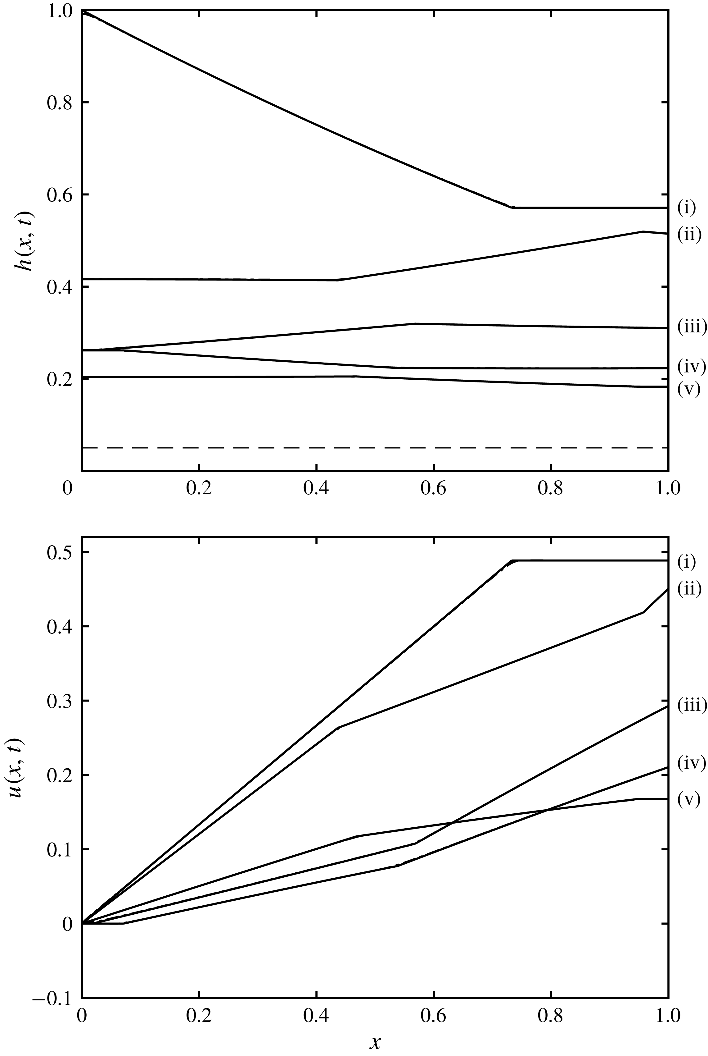
The height,
 $h(x,t)$
and velocity,
 $u(x,t)$
, as functions of position at various instances of time,
 $t=1,2,3,4$
and
 $5$
(labelled (i)–(v), respectively) for
 $D=0.05$
and
 $w=1$
. The solid line depicts the solution calculated using the quasi-analytical hodograph methods, while the dot-dashed line depicts the solution from the direct numerical integration of the shallow-water equations (2.1a
)–(2.1b
). We note that there is negligible difference between the curves, which overlie each other; the largest differences occur close to positions in the profiles where the solutions have discontinuous gradient. Such features are captured exactly by the analytical approach, whereas the numerical results are slightly smoothed. The dashed line indicates the height of the barrier
 $(D=0.05)$
.
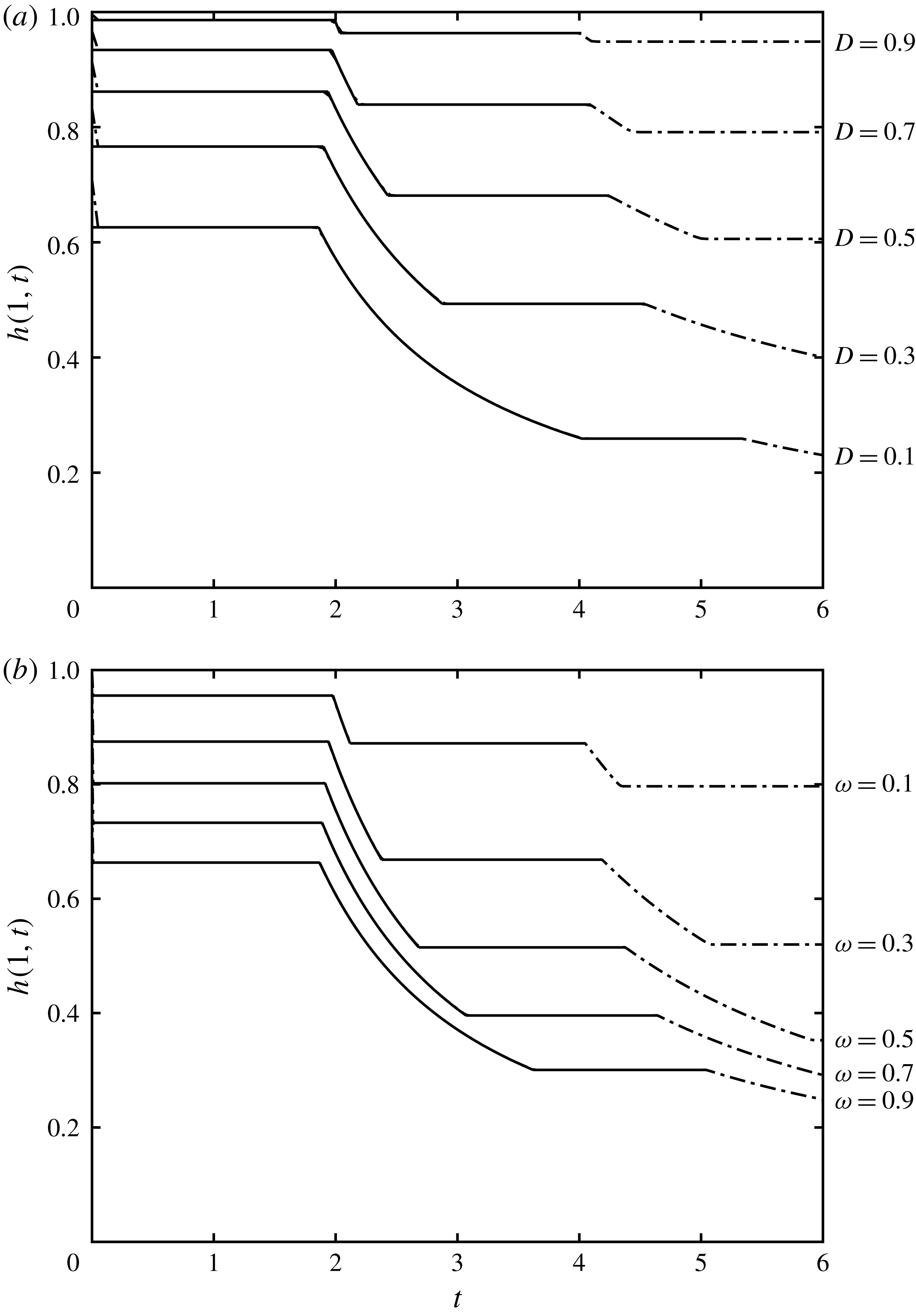
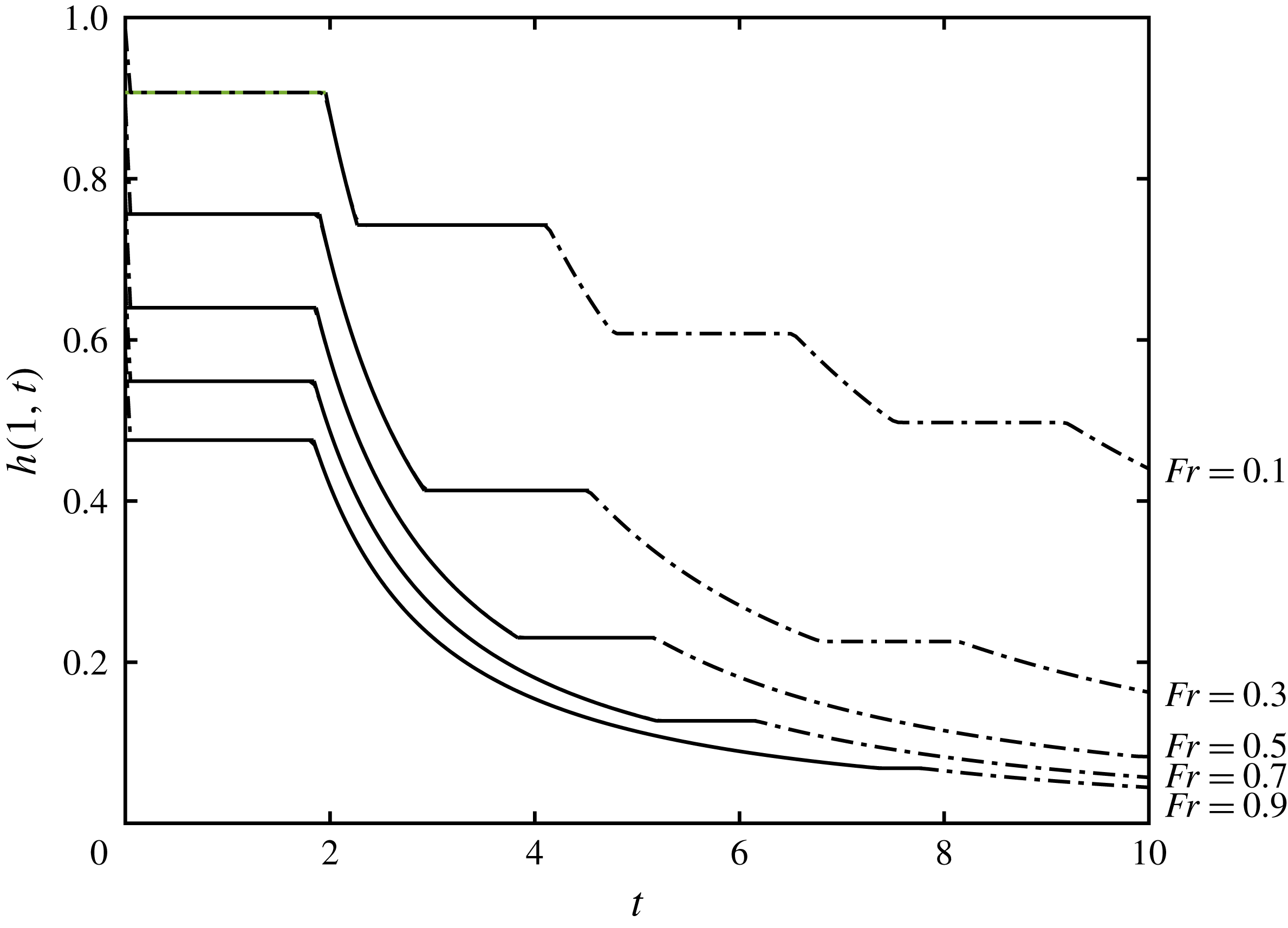
The height at the free-draining boundary,
 $h(1,t)$
, as a function of time for (a) various barrier heights,
 $D$
, and
 $w=1$
; and (b) various constrictions,
 $w$
, and
 $D=0.1$
. The solid lines correspond to results from integration in the hodograph plane and the dot-dashed lines correspond to numerical integration of the shallow water equations (2.1a
)–(2.1b
). The quasi-analytical hodograph calculations were performed until the end of region
 $U_{4}$
, but the numerical computations were continued over much longer times. We note the very close agreement between the two approaches, with the only very slight differences occurring at the junctions of the intervals during which the height is uniform or decreasing.

Given
 $t_{s}(\unicode[STIX]{x1D6FC})$
, the dependent variables can be evaluated immediately by numerical quadrature, using (3.14) for
 $t(\unicode[STIX]{x1D6FC},\unicode[STIX]{x1D6FD})$
and integrating along an
 $\unicode[STIX]{x1D6FC}$
-characteristic using (2.6a
) to determine
 $x(\unicode[STIX]{x1D6FC},\unicode[STIX]{x1D6FD})$
, with condition
 $x=x_{b3}$
. This enables the boundary to
 $C_{2}$
to be computed as the
 $\unicode[STIX]{x1D6FC}$
-characteristic on which
 $\unicode[STIX]{x1D6FC}=-\unicode[STIX]{x1D6FD}_{\ast }$
, starting from
 $P_{5}$
. The
 $\unicode[STIX]{x1D6FC}$
-characteristic reaches the free-draining boundary at
 $P_{6}=(1,t_{s}(-\unicode[STIX]{x1D6FD}_{\ast }))$
.
Finally we note that we also construct the characteristic on which
 $\unicode[STIX]{x1D6FC}=-\unicode[STIX]{x1D6FD}_{\ast }$
emanating from the point
 $P_{7}$
at the back wall. This curve denoted parametrically by
 $(x_{a3},t_{a3})$
is determined from the characteristic equation (2.6a
), which here yields
 $$\begin{eqnarray}\frac{\unicode[STIX]{x2202}x_{a3}}{\unicode[STIX]{x2202}\unicode[STIX]{x1D6FD}}=\frac{(-3\unicode[STIX]{x1D6FD}_{\ast }+\unicode[STIX]{x1D6FD})}{4}\frac{\unicode[STIX]{x2202}t_{a3}}{\unicode[STIX]{x2202}\unicode[STIX]{x1D6FD}}.\end{eqnarray}$$
Also in the simple wave region,
 $S_{3}$
, in which
 $\unicode[STIX]{x1D6FC}=-\unicode[STIX]{x1D6FD}_{\ast }$
, we have that
 $$\begin{eqnarray}\frac{x-x_{a2}}{t-t_{a2}}=\frac{-\unicode[STIX]{x1D6FD}_{\ast }+3\unicode[STIX]{x1D6FD}}{4}.\end{eqnarray}$$
Hence we deduce that
 $$\begin{eqnarray}t_{a3}-t_{a2}=-\frac{2}{\unicode[STIX]{x1D6FD}_{\ast }}x_{b3}(-\unicode[STIX]{x1D6FD}_{\ast })\left(\frac{-2\unicode[STIX]{x1D6FD}_{\ast }}{-\unicode[STIX]{x1D6FD}_{\ast }-\unicode[STIX]{x1D6FD}}\right)^{3/2},\end{eqnarray}$$
and then
 $x_{a3}$
follows from (3.17). The uniform region adjacent to the free-draining boundary corresponds to
 $(\unicode[STIX]{x1D6FC},\unicode[STIX]{x1D6FD})=(-\unicode[STIX]{x1D6FD}_{\ast },\unicode[STIX]{x1D6FD}_{m})$
, where
 $\unicode[STIX]{x1D6FD}_{m}=\unicode[STIX]{x1D6FD}_{s}(-\unicode[STIX]{x1D6FD}_{\ast })$
. Then we may determine
 $P_{8}$
as
 $(x_{a3}(\unicode[STIX]{x1D6FD}_{m}),t_{a3}(\unicode[STIX]{x1D6FD}_{m}))$
and
 $P_{9}$
as
 $(1,t_{a3}(\unicode[STIX]{x1D6FD}_{m})+4(1-x_{a3}(\unicode[STIX]{x1D6FD}_{m}))/(\unicode[STIX]{x1D6FD}_{m}-3\unicode[STIX]{x1D6FD}_{\ast }))$
.
The construction of the solution may be extended to the complex wave region
 $C_{3}$
using the boundary data along the
 $\unicode[STIX]{x1D6FC}$
- characteristic on which
 $\unicode[STIX]{x1D6FC}=-\unicode[STIX]{x1D6FD}_{\ast }$
; these data are
 $x_{a3}(\unicode[STIX]{x1D6FD})$
and
 $t=t_{a3}(\unicode[STIX]{x1D6FD})$
, and are derived above. In addition we enforce the impermeability of the back wall (2.2) by imposing symmetry on the
 $t$
-variable, so that
 $t(\unicode[STIX]{x1D6FC},\unicode[STIX]{x1D6FD})=t(-\unicode[STIX]{x1D6FD},-\unicode[STIX]{x1D6FC})$
. We then integrate around a rectangle in the hodograph plane,
 $VWXY$
, with edges aligned with the coordinate axes (see figure 4). The vertices of the rectangle are at
 $V=(-\unicode[STIX]{x1D6FD}_{\ast },\unicode[STIX]{x1D6FD}_{\ast })$
,
 $W=(\unicode[STIX]{x1D6FC},\unicode[STIX]{x1D6FD}_{\ast })$
,
 $X=(\unicode[STIX]{x1D6FC},\unicode[STIX]{x1D6FD})$
and
 $Y=(-\unicode[STIX]{x1D6FD}_{\ast },\unicode[STIX]{x1D6FD})$
. The characteristic data
 $t=t_{a3}(\unicode[STIX]{x1D6FD})$
provide the solution on the boundary segment
 $YV$
, while the imposed symmetry determines the solution on the boundary segment
 $VW$
,
 $t(\unicode[STIX]{x1D6FC},\unicode[STIX]{x1D6FD}_{\ast })=t(-\unicode[STIX]{x1D6FD}_{\ast },-\unicode[STIX]{x1D6FC})=t_{a3}(-\unicode[STIX]{x1D6FC})$
. We may then integrate (2.8) around
 $VWXY$
to yield
 $$\begin{eqnarray}\displaystyle t(\unicode[STIX]{x1D6FC},\unicode[STIX]{x1D6FD}) & = & \displaystyle B(\unicode[STIX]{x1D6FC},\unicode[STIX]{x1D6FD}_{\ast };\unicode[STIX]{x1D6FC},\unicode[STIX]{x1D6FD})t_{a3}(-\unicode[STIX]{x1D6FC})+B(-\unicode[STIX]{x1D6FD}_{3},\unicode[STIX]{x1D6FD};\unicode[STIX]{x1D6FC},\unicode[STIX]{x1D6FD})t_{a3}(\unicode[STIX]{x1D6FD})\nonumber\\ \displaystyle & & \displaystyle -\,B(-\unicode[STIX]{x1D6FD}_{\ast },\unicode[STIX]{x1D6FD}_{\ast };\unicode[STIX]{x1D6FC},\unicode[STIX]{x1D6FD})t_{a3}(\unicode[STIX]{x1D6FD}_{\ast })-I_{1}-I_{2},\end{eqnarray}$$
where the integrals
 $I_{1}$
and
 $I_{2}$
are given by
 $$\begin{eqnarray}\displaystyle & \displaystyle I_{1}=\int _{-\unicode[STIX]{x1D6FD}_{\ast }}^{\unicode[STIX]{x1D6FC}}\left(-\frac{3B}{2(a-\unicode[STIX]{x1D6FD}_{\ast })}+\frac{\unicode[STIX]{x2202}B}{\unicode[STIX]{x2202}a}\right)t_{a3}(-a)\,\text{d}a, & \displaystyle\end{eqnarray}$$
 $$\begin{eqnarray}\displaystyle & \displaystyle I_{2}=\int _{\unicode[STIX]{x1D6FD}}^{\unicode[STIX]{x1D6FD}_{\ast }}\left(-\frac{3B}{2(-\unicode[STIX]{x1D6FD}_{\ast }-b)}-\frac{\unicode[STIX]{x2202}B}{\unicode[STIX]{x2202}b}\right)t_{a3}(b)\,\text{d}b. & \displaystyle\end{eqnarray}$$
In the integrand of
 $I_{1}$
,
 $b=\unicode[STIX]{x1D6FD}_{\ast }$
, whereas in the integrand of
 $I_{2}$
,
 $a=-\unicode[STIX]{x1D6FD}_{\ast }$
. This construction is essentially the same as was used to derive (3.4) (Hogg Reference Hogg2006). The evaluation of
 $x(\unicode[STIX]{x1D6FC},\unicode[STIX]{x1D6FD})$
follows immediately by integrating along
 $\unicode[STIX]{x1D6FC}$
-characteristics (2.6a
) and using the boundary condition that
 $x(\unicode[STIX]{x1D6FC},-\unicode[STIX]{x1D6FC})=0$
.
The description of the solution presented in the previous paragraphs completes the computation of the flow fields for the first three reflections; subsequent reflections could in principle be computed using an identical formulation to find the complex wave regions next to the free-draining boundary and then to calculate the solutions close to the back wall. In the hodograph plane we can see that this sequence of regions forms an infinite ‘staircase’ towards the final state in which the fluid is quiescent of a flow depth equal to the height of the barrier. Notably, each reflection will generate uniform regions adjacent to the boundaries.
We illustrate the solution by plotting the solutions for the height and velocity fields as function of position at various fixed times for
 $D=0.05$
(see figure 5). The profiles, plotted at times
 $t=1,2,3,4$
and
 $5$
, draw from the uniform, simple and complex wave regions illustrated in figure 2. We note that they feature the uniform regions adjacent to the boundaries and that they illustrate the wave reflections along the reservoir. For example, we see that the flow oscillates so that at times it is thickest close to the end wall, while at other times it is thickest close to the free-draining boundary. We also plot the height at the draining boundary,
 $h(1,t)$
, as a function of time for various barrier heights and a constant width,
 $w=1$
, (figure 6
a) and for various constrictions and a constant barrier height,
 $D=0.1$
(figure 6
b). We note that this height at the end of the channel has intervals within which it is constant, followed by periods within which it declines; this is in accord with the description that we have developed above. The successive wave reflections lead to uniform regions adjacent to the boundaries within which the height and velocity are constant; in figure 6, we observe the height variation within regions,
 $U_{1}$
,
 $C_{2}$
and
 $U_{4}$
(see figure 2) and we have calculated these using the techniques described above. In principle we could extend this further, but in this study we access later times numerically and through using a different analytical approach (§ 3.3).
3.3 Late times: numerical results and asymptotic analysis
From the structure of the hodograph solution we anticipate that at late times we will continue to see a ‘staircase’ of uniform and complex wave regions. This is consistent with our numerical simulations, computed up to time
 $t=100$
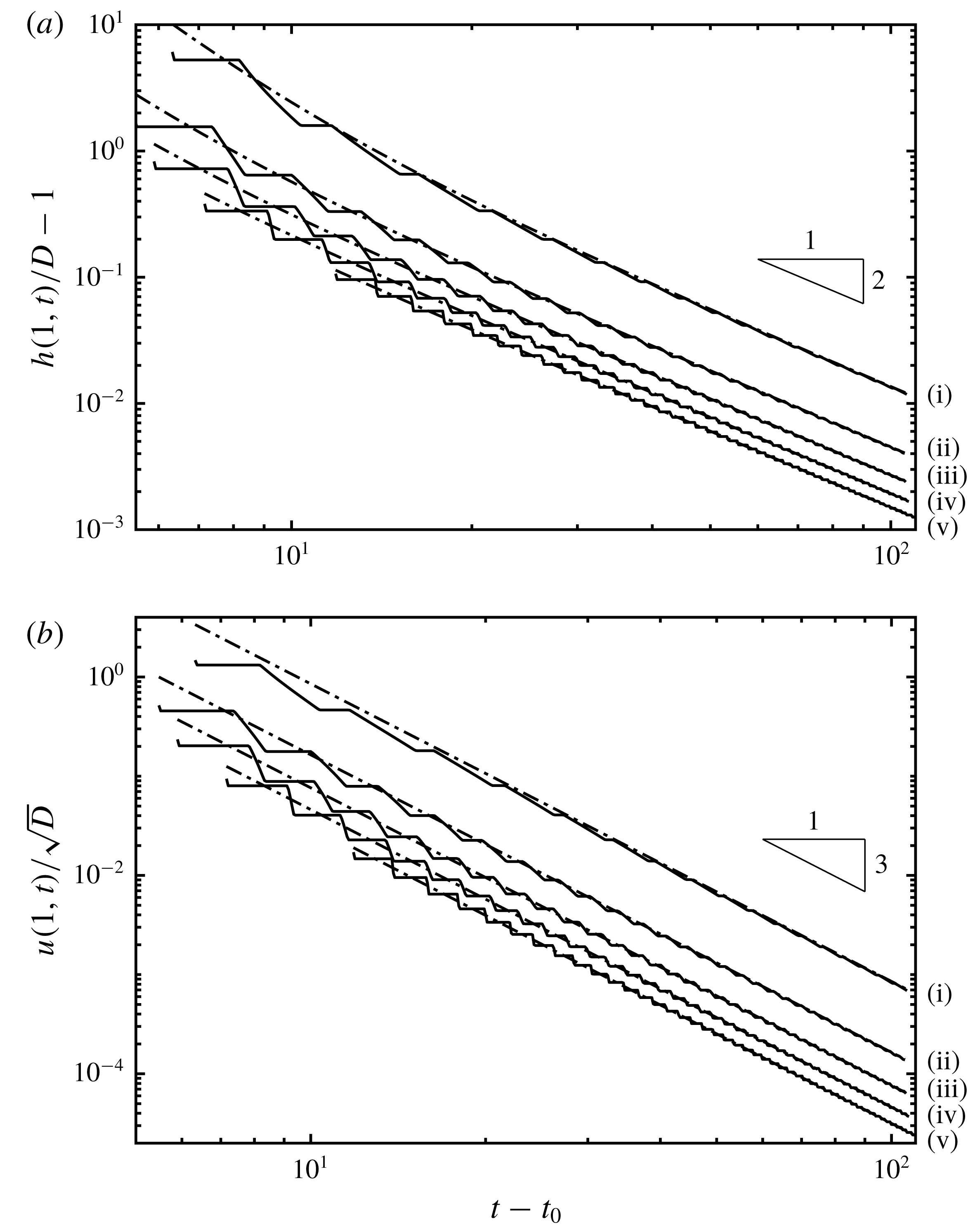
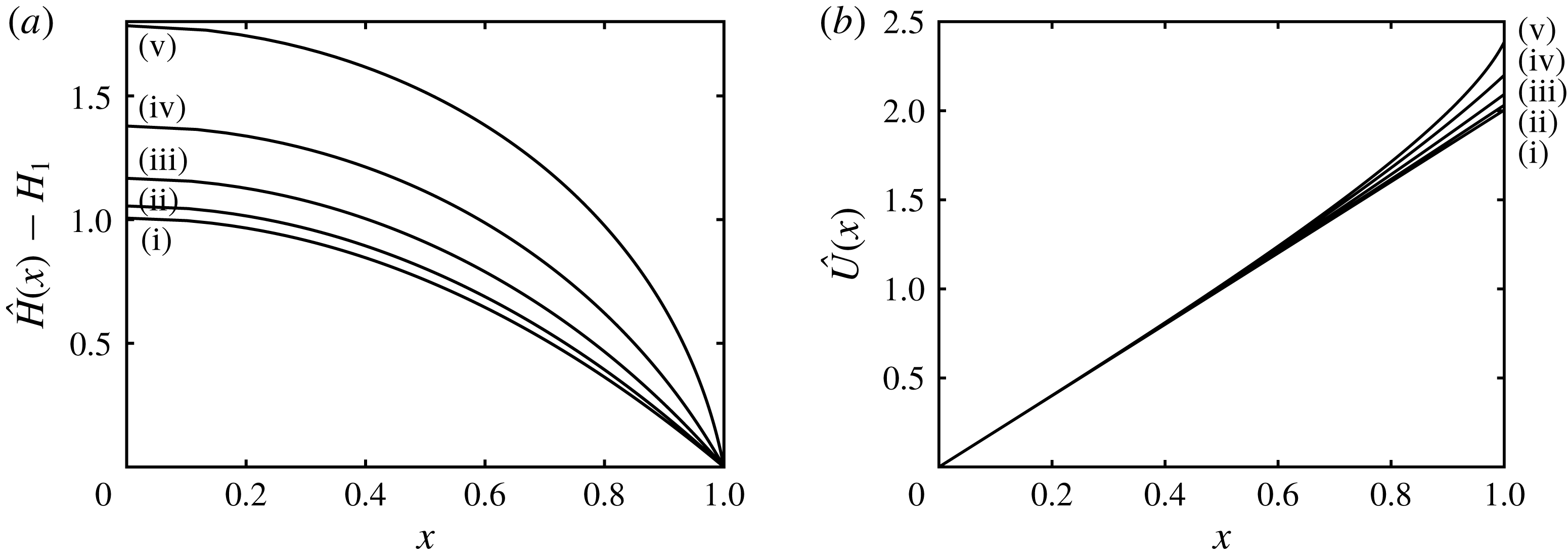
, and presented in figure 7. In this figure we plot the height excess over the barrier and the velocity incident on the barrier as functions of time for a selection of barrier heights. (We have introduced a time offset,
 $t_{0}$
and have also plotted the asymptotic trends, which are introduced and deduced below.) It is evident from these plots that the solution tends rapidly towards a power law, around which there are strong, but decaying, oscillations, whose period and shape are functions of the barrier height,
 $D$
.
In what follows we investigate the asymptotic form of the solutions for the height and velocity fields trends at late times after the flow initiation. For this analysis we utilise a multi-scale asymptotic expansion in time to capture the progressive unsteady draining of the reservoir and the more rapid oscillations, the amplitude of which decay temporally and the phase speed of which approach a constant value dependent upon the barrier height. This analysis is based upon embedding a set of time scales into the dependent variables and then examining their evolution at relatively late times. We first construct these appropriate time scales, then present the resulting expansion with the algebraic details confined to appendix B. Finally we compare the asymptotic forms to the numerical simulations.
(a) The elevation of the fluid layer above the barrier relative to the height of the barrier,
 $h(1,t)/D-1$
; and (b) and the velocity at the outflow
 $u(1,t)/\sqrt{D}$
as functions of time for
 $w=1$
and
 $D=0.9,0.7,0.5,0.3,0.1$
(denoted (i)–(v), respectively). The solid lines are from numerical integration of the governing equations and reveal strong oscillatory behaviour superimposed upon progressive decay of each variable. The dashed-dot lines are the single-scale asymptotic solution from (3.26a,b
).

We investigate the solution at late times, where
 $t=O(1/\unicode[STIX]{x1D716})$
and
 $\unicode[STIX]{x1D716}$
is a small, arbitrary ordering parameter
 $(0<\unicode[STIX]{x1D716}\ll 1)$
. In the end, the solutions cannot depend upon
 $\unicode[STIX]{x1D716}$
, but its introduction is useful in organising the magnitude of various terms. We also introduce the following set of time scales,
 $\hat{T}_{n}(\unicode[STIX]{x1D716},t)$
 $(n=0,1,2,\ldots )$
, such that at the long time scale of interest
 $\hat{T}_{n}=O(\unicode[STIX]{x1D716}^{n-1})$
. Provided that all variables other than
 $t$
and
 $\hat{T}_{n}$
are independent of
 $\unicode[STIX]{x1D716}$
we can always express the time scales as
 $$\begin{eqnarray}\hat{T}_{n}(\unicode[STIX]{x1D716},t)=\unicode[STIX]{x1D716}^{n-1}\unicode[STIX]{x1D714}_{n}(\unicode[STIX]{x1D716}t),\end{eqnarray}$$
where
 $\unicode[STIX]{x1D714}_{n}$
are functions of order unity when
 $t=O(1/\unicode[STIX]{x1D716})$
. For the purposes of constructing an asymptotic expansion the time scale
 $\hat{T}_{1}=\unicode[STIX]{x1D714}_{1}(\unicode[STIX]{x1D716}t)$
is equivalent to
 $\tilde{T}_{1}=\unicode[STIX]{x1D716}t$
. Therefore, without loss of generality, we take
 $$\begin{eqnarray}\hat{T}_{0}=\unicode[STIX]{x1D716}^{-1}\unicode[STIX]{x1D714}_{0}(T_{1}),\quad \hat{T}_{1}=\unicode[STIX]{x1D716}t,\quad \hat{T}_{n}=\unicode[STIX]{x1D716}^{n-1}\unicode[STIX]{x1D714}_{n}(T_{1}),\quad n\in \{2,3,\ldots \},\end{eqnarray}$$
where
 $\unicode[STIX]{x1D714}_{n}^{\prime }\neq 0$
,
 $n\in \{0,2,3,\ldots \}$
.
For most problems multi-scale asymptotics fails to produce a closed system of equations for high-order corrections involving high-order time scales, as mentioned in Bender & Orszag (Reference Bender and Orszag1999, § 11.2). To understand why this is, we consider a problem in
 $m$
time scales which, at each order, generates
 $r$
new arbitrary functions dependent on
 $m-1$
time scales (the dependence on one of the time scales being set at that order), along with
 $s$
solvability conditions providing restrictions on the functions introduced at lower order. Considering an expansion including
 $N$
terms, and ignoring contributions independent of
 $N$
, this means there is a total of
 $r(m-1)N$
functional dependencies and
 $sN$
solvability conditions, resulting in
 $[r(m-1)-s]N$
undetermined dependencies. To stress how pathologically bad this lack of closure is, we observe that if a full set of
 $O(N)$
time scales is used then we will have
 $O(N^{2})$
undetermined dependencies. If we are to have a closed expansion, introducing the same number of dependencies and conditions as we increase from order
 $N$
to
 $N+1$
, we must have
 $m=1+s/r$
.
For many problems, such as the one considered here,
 $s=a$
and thus we require two time scales. We anticipate that, as with many of the problems discussed in Kevorkian & Cole (Reference Kevorkian and Cole1996), the time scale
 $\hat{T}_{0}$
is the time scale in which oscillations and waves occur,
 $\hat{T}_{1}$
governs the amplitude of these waves, and higher-order time scales act as a phase shift to
 $\hat{T}_{0}$
in the form of a strained coordinate (Hinch Reference Hinch1992, § 7.1). This results in the two-scale ansatz: that all time dependencies can be expressed by the time scales
 $$\begin{eqnarray}\displaystyle & \displaystyle T_{0}=k_{0}\hat{T}_{0}+k_{2}\hat{T}_{2}+k_{3}\hat{T}_{3}+\cdots =\unicode[STIX]{x1D716}^{-1}\unicode[STIX]{x1D714}_{0}(T_{1})+\unicode[STIX]{x1D716}\unicode[STIX]{x1D714}_{2}(T_{1})+\unicode[STIX]{x1D716}^{2}\unicode[STIX]{x1D714}_{3}(T_{1})+\cdots \,,\qquad & \displaystyle\end{eqnarray}$$
 $$\begin{eqnarray}\displaystyle & \displaystyle T_{1}=\hat{T}_{1}=\unicode[STIX]{x1D716}t, & \displaystyle\end{eqnarray}$$
 $k_{n}$
have been absorbed into
 $\unicode[STIX]{x1D714}_{n}$
.
Our asymptotic analysis then proceeds by assuming that the height and velocity fields are dependent on both time scales
 $T_{0}$
and
 $T_{1}$
as well as the spatial variable
 $x$
. We substitute series expansion of the form (B 9b
) into the governing equations (2.1a
)–(2.1b
) and deduce expressions that satisfy the boundary conditions and remain bounded as time evolves. These latter ‘secular’ conditions are key to determining the functions,
 $\unicode[STIX]{x1D714}_{n}$
, and the decaying amplitudes of the wave-like behaviour.
It is convenient to write the solutions for the dependent fields as the sum of two contributions,
 $$\begin{eqnarray}h=h_{a}+h_{w}\quad \text{and}\quad u=u_{a}+u_{w},\end{eqnarray}$$
where
 $h_{a}$
and
 $u_{a}$
are asymptotic components of the solutions that depend on
 $T_{1}$
(and will be henceforth termed the ‘single time-scale asymptotics’) and
 $h_{w}$
and
 $u_{w}$
are the wave-like components. From appendix B, we find that correct to
 $O(1/(\sqrt{D}(t-t_{0}))^{5})$
 $$\begin{eqnarray}\displaystyle & \displaystyle \frac{h_{a}(x,t)}{D}=1+\frac{27}{2w^{2}(\sqrt{D}(t-t_{0}))^{2}}+\frac{27(3x^{2}+5)}{2w^{2}(\sqrt{D}(t-t_{0}))^{4}}, & \displaystyle\end{eqnarray}$$
 $$\begin{eqnarray}\displaystyle & \displaystyle \frac{u_{a}(x,t)}{\sqrt{D}}=\frac{27x}{w^{2}(\sqrt{D}(t-t_{0}))^{3}}, & \displaystyle\end{eqnarray}$$
 $$\begin{eqnarray}\displaystyle \frac{h_{w}(x,t)}{D} & = & \displaystyle \frac{1}{(\sqrt{D}(t-t_{0}))^{3}}[F(\unicode[STIX]{x1D702})+F(\unicode[STIX]{x1D709})]\nonumber\\ \displaystyle & & \displaystyle +\,\frac{1}{(\sqrt{D}(t-t_{0}))^{4}}\left[\frac{w^{2}}{9}(F(\unicode[STIX]{x1D702})^{2}+F(\unicode[STIX]{x1D709})^{2})+3x(F(\unicode[STIX]{x1D702})-F(\unicode[STIX]{x1D709}))\right],\qquad\end{eqnarray}$$
 $$\begin{eqnarray}\displaystyle \frac{u_{w}(x,t)}{\sqrt{D}} & = & \displaystyle \frac{1}{(\sqrt{D}(t-t_{0}))^{3}}[F(\unicode[STIX]{x1D702})-F(\unicode[STIX]{x1D709})]\nonumber\\ \displaystyle & & \displaystyle +\,\frac{1}{(\sqrt{D}(t-t_{0}))^{4}}\left[\frac{w^{2}}{9}(F(\unicode[STIX]{x1D702})^{2}-F(\unicode[STIX]{x1D709})^{2})+3x(F(\unicode[STIX]{x1D702})+F(\unicode[STIX]{x1D709}))\right],\qquad\end{eqnarray}$$
 $$\begin{eqnarray}\unicode[STIX]{x1D709}(x,t)=\sqrt{D}t-\frac{27}{4w^{2}\sqrt{D}(t-t_{0})}+x,\quad \text{and}\quad \unicode[STIX]{x1D702}(x,t)=\sqrt{D}t-\frac{27}{4w^{2}\sqrt{D}(t-t_{0})}-x.\quad\end{eqnarray}$$
The variable
 $t_{0}$
denotes a temporal offset that we are free to choose. The arbitrary function
 $F$
is related to the initial conditions that gave rise to the unsteady draining flow. In terms of the variables in the appendix B, it is given by
 $F(y)=D\hat{F}_{3}(y-\sqrt{D}\unicode[STIX]{x1D719})$
, and is thus of period
 $2$
. The function is affected by the choice of
 $t_{0}$
via the transformation
 $$\begin{eqnarray}t_{0}\mapsto t_{0}+k,\quad \text{leads to }F\mapsto F+\frac{27k}{2\sqrt{D}w^{2}}.\end{eqnarray}$$
Thus we may choose
 $F$
to have zero integral over each period by choosing
 $t_{0}$
, which means that the wave component oscillates around the single-scale component. From (3.26) we see that
 $D$
only affects the scales of
 $h$
,
 $u$
and
 $t$
, which is equivalent to choosing to make the variables dimensionless with respect to
 $HD$
rather than
 $H$
. The constant small parameter
 $\unicode[STIX]{x1D716}$
used to compute the solution at the time
 $t$
must have magnitude approximately
 $1/t$
for
 $\unicode[STIX]{x1D716}t$
to be order unity. We define the time dependent small parameter
 $\unicode[STIX]{x1D716}_{t}$
to mean the value of
 $\unicode[STIX]{x1D716}$
which rescales
 $t$
to exactly unity, taking into account appropriate scales and offset, that is
 $$\begin{eqnarray}\unicode[STIX]{x1D716}_{t}=\frac{1}{\sqrt{D}(t-t_{0})}.\end{eqnarray}$$
We compare these asymptotic results with the numerical simulations as follows: we suppose that we know
 $t_{0}$
as well as the dependent variables at some comparison time
 $t=t_{c}$
, given by
 $h(x,t_{c})$
,
 $u(x,t_{c})$
, and we use these fields to determine the function
 $F$
over a single period. The differences between the numerically computed fields and the single-scale asymptotic components,
 $h_{wn}=h(x,t_{c})-h_{a}(x,t_{c})$
and
 $u_{wn}=u(x,t_{c})-u_{a}(x,t_{c})$
are added and subtracted to give
 $$\begin{eqnarray}\displaystyle \frac{h_{wn}(x,t_{c})}{2D}+\frac{u_{wn}(x,t_{c})}{2\sqrt{D}} & = & \displaystyle \frac{F(\unicode[STIX]{x1D702}_{c})}{(\sqrt{D}(t_{c}-t_{0}))^{3}}\nonumber\\ \displaystyle & & \displaystyle +\,\frac{1}{(\sqrt{D}(t_{c}-t_{0}))^{4}}\left[\frac{w^{2}F(\unicode[STIX]{x1D702}_{c})^{2}}{9}+3xF(\unicode[STIX]{x1D702}_{c})\right],\end{eqnarray}$$
 $$\begin{eqnarray}\displaystyle \frac{h_{wn}(x,t_{c})}{2D}-\frac{u_{wn}(x,t_{c})}{2\sqrt{D}} & = & \displaystyle \frac{F(\unicode[STIX]{x1D709}_{c})}{(\sqrt{D}(t_{c}-t_{0}))^{3}}\nonumber\\ \displaystyle & & \displaystyle +\,\frac{1}{(\sqrt{D}(t_{c}-t_{0}))^{4}}\left[\frac{w^{2}F(\unicode[STIX]{x1D709}_{c})^{2}}{9}-3xF(\unicode[STIX]{x1D709}_{c})\right],\end{eqnarray}$$
 $\unicode[STIX]{x1D709}_{c}(x)=\unicode[STIX]{x1D709}(x,t_{c})$
,
 $\unicode[STIX]{x1D702}_{c}(x)=\unicode[STIX]{x1D702}(x,t_{c})$
. These expressions apply for
 $0\leqslant x\leqslant 1$
. We may write (3.30a
) and (3.30b
) in a compact way by introducing the period 2 function
 $S(y)$
, defined by
 $$\begin{eqnarray}S(y)=(\sqrt{D}(t_{c}-t_{0}))^{3}\left[\frac{h_{wn}(|\unicode[STIX]{x1D712}|,t_{c})}{2D}-\operatorname{sgn}(\unicode[STIX]{x1D712})\frac{u_{wn}(|\unicode[STIX]{x1D712}|,t_{c})}{2\sqrt{D}}\right],\end{eqnarray}$$
where
 $y=\sqrt{D}t_{c}-27/(4w^{2}\sqrt{D}(t_{c}-t_{0}))+\unicode[STIX]{x1D712}$
and
 $-1<\unicode[STIX]{x1D712}<1$
. Therefore the function
 $F$
satisfies the following quadratic equation,
 $$\begin{eqnarray}F^{2}(y)-2BF(y)-C=0,\end{eqnarray}$$
where
 $$\begin{eqnarray}B=\frac{27\unicode[STIX]{x1D712}-9\sqrt{D}(t_{c}-t_{0})}{2w^{2}},\quad \text{and}\quad C=\frac{9\sqrt{D}(t_{c}-t_{0})}{w^{2}}S(y).\end{eqnarray}$$
We expect that
 $F\sim S$
for
 $t_{c}\gg t_{0}$
, which selects the solution to (3.32) given by
 $$\begin{eqnarray}F=B+\sqrt{B^{2}+C}.\end{eqnarray}$$
Finally, we evaluate the temporal offset,
 $t_{0}$
, by imposing
 $$\begin{eqnarray}\int _{0}^{2}F(y)\,\text{d}y=0.\end{eqnarray}$$
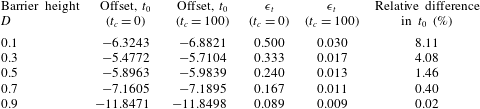
In table 1 we present the evaluation of the temporal offset,
 $t_{0}$
, for various barrier heights,
 $D$
, and uniform width,
 $w=1$
, using either the initial conditions
 $(t_{c}=0)$
or the numerically determined profiles at
 $t_{c}=100$
. We find that the two values of
 $t_{0}$
for each barrier height are broadly similar; the relative difference is less than
 $10\,\%$
and systematically decreases with
 $D$
. The computed value of
 $\unicode[STIX]{x1D716}_{t}$
given in table 1 according to (3.29) provides an indication of the magnitude of the difference between the numerically computed profiles and their asymptotic forms. Indeed we find that even using the initial conditions
 $(t_{c}=0)$
to determine
 $t_{0}$
appears to provide an accurate means of determining the asymptotic form for the larger barrier heights (
 $D\gtrsim 0.5$
).
The temporal offset,
 $t_{0}$
, for various values of the barrier height
 $D$
with
 $w=1$
, computed using (3.35) enforced at time
 $t_{c}=0$
and
 $t_{c}=100$
. (For the latter, the dependent variables,
 $h$
and
 $u$
, were evaluated from the numerical simulations.) The corresponding values of
 $\unicode[STIX]{x1D716}_{t}$
are also given, along with the relative difference in the two computed values of
 $t_{0}$
.

In figure 7 we have plotted the single time-scale asymptotics,
 $h_{a}$
and
 $u_{a}$
(see (3.26a
)–(3.26b
)) as functions of time at the end of the domain
 $(x=1)$
. For these plots we evaluated the temporal offset using the initial data
 $(t_{c}=0)$
. We observe that these asymptotic forms accurately capture the numerical computations over relatively long computational times, and thus at late times for all barrier heights the outflow velocity decays with the inverse cube of time, whereas the excess height decays as the inverse square of time. We further note that there are oscillations of diminishing amplitude about the progressive decay of the height and velocity fields, which in these figures correspond to periods during which the outflow velocity and height remain constant; these oscillations are captured in the wave-like behaviour,
 $h_{w}$
and
 $u_{w}$
and are discussed below.
At late times when the depth of the fluid at the outflow is close to the barrier height
 $(h-D\ll 1)$
, we find that the velocity field satisfies
 $u\sim w(h-D)^{3/2}/D$
. Thus the flow speed is weakening and eventually viscous stresses, which are not included in the dynamical model, may become non-negligible. We show in appendix A how to assess their magnitude within the shallow flow over the crest of the weir and for the typical parameter values at environmental scales, viscous effects appear negligible until
 $h-D\sim 10^{-3}$
.
The rescaled volume flux at the outflow boundary,
 $u(1,t)h(1,t)/D^{3/2}$
is plotted in figure 8 as a function of rescaled time
 $\sqrt{D}(t-t_{0})$
for various values of the barrier height,
 $D$
. In this plot we have calculated the offset time,
 $t_{0}$
from the initial profile (i.e.
 $t_{c}=0$
), according to the procedure described above; values of
 $t_{0}$
are given as the second column of table 1. We note that for
 $\sqrt{D}(t-t_{0})\gtrsim 4$
, the evolution follows a universal behaviour around which each of the separate cases oscillate due to the successive wave reflections between the back wall and the outflow. Furthermore we have also plotted the analytically calculated asymptotic form,
 $u_{a}(1,t)h_{a}(1,t)/D^{3/2}$
, where
 $h_{a}$
and
 $u_{a}$
are given by (3.26a
) and (3.26b
), respectively. We observe that this expression accurately matches the computed flux.
The rescaled volume flux of fluid leaving the domain at the outflow,
 $u(1,t)h(1,t)/D^{3/2}$
, as a function of rescaled time
 $\sqrt{D}(t-t_{0})$
with the temporal offset,
 $t_{0}$
, calculated from the initial profile, for
 $D=0.1,0.3,0.5,0.7$
and
 $0.9$
(solid lines) and
 $w=1$
. The asymptotic form,
 $u_{a}(1,t)h_{a}(1,t)/D^{3/2}$
, is plotted with a dot-dashed line. In this figure, the curves from the different numerical computations overlay at late times and it is hard to distinguish them, indicating a universal behaviour that is accurately represented by the asymptotic form.

The shape of the waveform of the oscillations can also be determined asymptotically and may in some cases be deduced from the initial conditions. When
 $t_{c}=0$
, the fluid is stationary
 $(u(x,t_{c})=0)$
and the reservoir is of unit depth
 $(h(x,t_{c})=1)$
. In this case using the transform (3.28) and enforcing (3.35) we arrive at
 $$\begin{eqnarray}F(y)=\frac{27\unicode[STIX]{x1D712}}{2w^{2}}\equiv \frac{27}{2w^{2}}\left(y-\sqrt{D}t_{c}+\frac{27}{4w^{2}\sqrt{D}(t_{c}-t_{0})}\right)\end{eqnarray}$$
for
 $-1<\unicode[STIX]{x1D712}<1$
. This function, constructed to be periodic, contains a discontinuity at
 $\unicode[STIX]{x1D712}=\pm 1$
. This is exactly the same as what would be produced if we had truncated our asymptotic expansion at a lower order and included terms up to
 $(t-t_{0})^{-3}$
. To understand this observation, we note that the rarefaction fan which smooths out the mismatch between the initial conditions and boundary condition at early times only exists because of the nonlinearity of the shallow water equations. A linear system of hyperbolic partial differential equations would simply advect this mismatch as a discontinuity. Thus, we should only expect the asymptotic solution to capture this smoothing behaviour if we expand to sufficiently high order to capture the nonlinear interaction of the waves, and to calculate (3.26) we only expanded to capture the nonlinear effects of the boundary conditions and single-scale component, not the wave component. We therefore find that the asymptotic solution simply advects the initial mismatch as a discontinuity (which is what we see in figure 9). This failure to capture the nonlinear self-interaction of the waves means we fail to capture the correct wave shape over the first few periods. We explore this effect by making comparisons between the simulation and asymptotic solution at a number of early times to find the time at which the nonlinear effects become small and consequentially the simulation results are accurately represented by the asymptotic expressions.
The waveform of the oscillation at long times,
 $F$
, for barrier of heights (a)
 $D=0.1$
; (b)
 $0.5$
; (c)
 $0.7$
; and (d)
 $0.9$
and for
 $w=1$
. In each figure, the waveform is extracted from the numerical simulations at seven comparison times
 $t_{c}$
. For each case the waveforms converge to a single profile when
 $t_{c}$
becomes sufficiently large, in accord with the asymptotic analysis. In (d) the waveform at late times is quite close to the waveform deduced from initial conditions (
 $t_{c}=0$
, dot-dashed line), but for (a–c) there are differences due to appreciable nonlinear interactions during the initial phases of the motion.
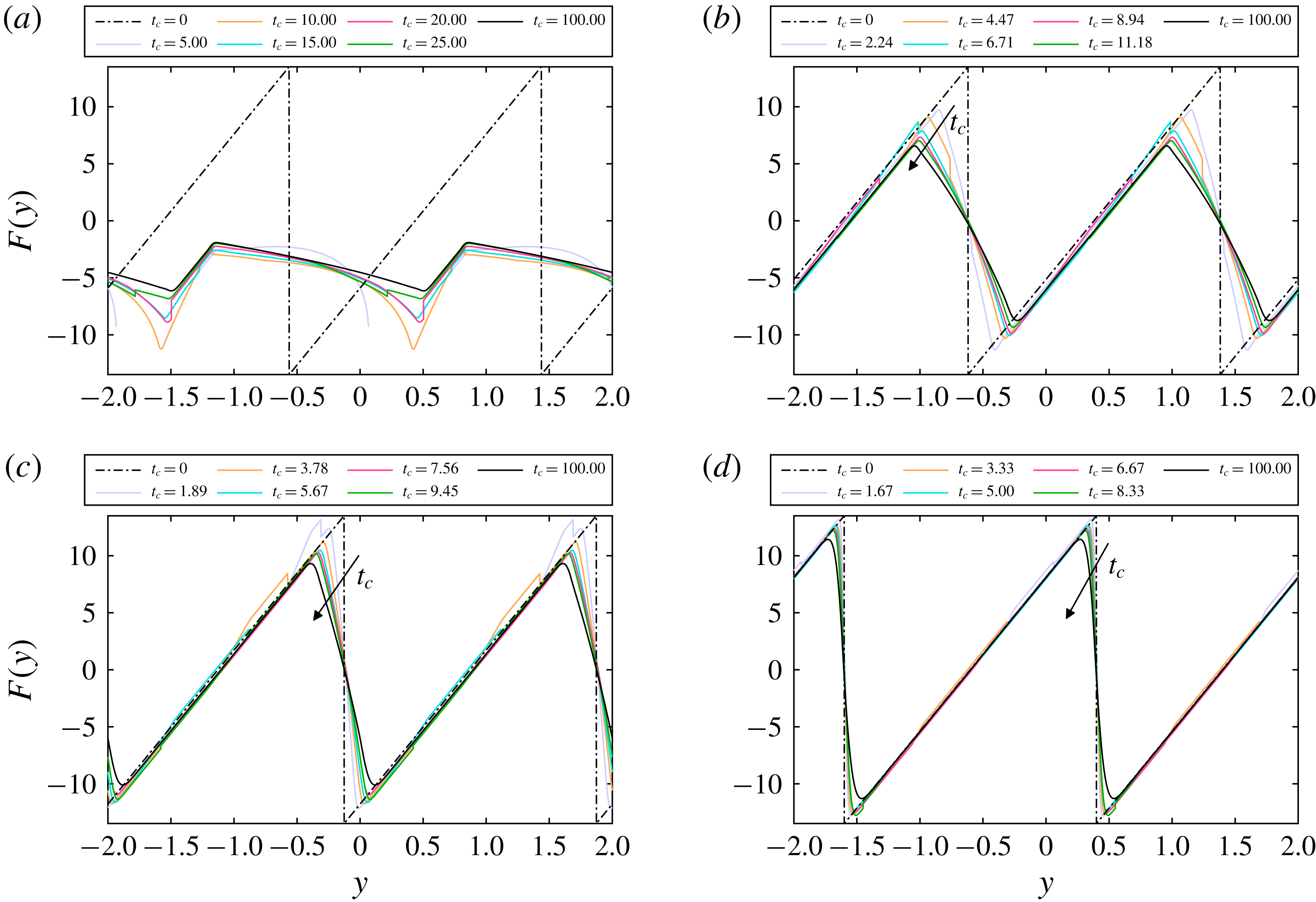
Figure 9 shows the waveform
 $F(y)$
as computed from the numerical simulations for a selection of barrier heights,
 $D$
, and comparison times,
 $t_{c}$
with
 $w=1$
. (The curve at
 $t_{c}=0$
is given by (3.36) in each case.) For all cases, as time passes, the wave seen in the simulation converges on a time-independent shape, which is in accord with the asymptotic analysis. Indeed this confirms that the amplitude of the wave-like part of the dependent fields,
 $h_{w}$
and
 $u_{w}$
, decays as
 $(t-t_{0})^{-3}$
and that the phase speed approaches
 $\sqrt{D}$
(see (3.26c
) and (3.26d
)). In fact we observe for
 $\sqrt{D}(t_{c}-t_{0})\gtrsim 10$
there is very little change in the computed shape of
 $F$
, indicating that by that stage the numerical results are accurately approximated by the asymptotic form. We now discuss the figures in order of increasing
 $\unicode[STIX]{x1D716}_{t}$
(see table 1), i.e. most accurate to least accurate.
Figure 9(d) shows that for relatively large values of
 $D$
, the asymptotic expansion based upon
 $t_{c}=0$
accurately predicts the numerically computed phase speed and the wave shape. Figures 9(c) and 9(d), in contrast, reveal some discrepancies. Examining the portions with positive gradient (which correspond to uniform and simple wave regions in the hodograph solution) we see excellent correspondence between different times suggesting that we have both the correct phase speed and wave shape for these portions. However, the portions with negative gradient (corresponding to simple and complex wave regions) are not very accurate, and these are precisely the regions in which the nonlinear wave self-interaction is important. Figure 9(a) reveals that for relatively small values of
 $D$
, we do not have the correct wave phase speed for early times, because the simulated waveform drifts off of the predicted wave even in the positive gradient regions. Furthermore it is evident that the calculation of the waveform
 $F$
from the initial conditions
 $(t_{c}=0)$
does not provide a useful indication of the behaviour at later times. Instead one must deduce the asymptotic form from the profiles at later times,
 $t_{c}$
, or one must employ a higher-order expansion, to predict the phase speed accurately.
4 Draining through a constriction
In this section we compute the unsteady drainage that occurs through a constriction at one end of the reservoir. In this situation, the drainage boundary condition is given by (2.3) with
 $D=0$
and
 $0<w\leqslant 1$
, which may be written
 $$\begin{eqnarray}w=Fr\left(\frac{3}{Fr^{2}+2}\right)^{3/2}.\end{eqnarray}$$
Thus given a relative width of the constriction,
 $w$
, we may determine the Froude number and this remains constant throughout the entire motion. We demonstrate below that many of the features of the unsteady flow over a barrier are reproduced for the current scenario of flows through constrictions, importantly including the successive nonlinear wave reflections from the back wall and drainage boundary. There are differences, however, in the evolution at long times; for flows through a constriction, the depth of the fluid layer ultimately vanishes and does so in a self-similar way, reflecting the absence of any additional length scales in the shallow-water model of the motion. We construct the solutions for the motion using the hodograph transformation and the method of characteristics, numerical computations and we derive and assess the linear stability of the similarity solution that governs the dynamics at late times.
The characteristic plane for the unsteady draining of fluid from a partially confined reservoir with constriction width,
 $w=4/3^{3/2}$
and Froude number
 $Fr=0.5$
. In this figure we plot and label the uniform, simple and complex wave regions following the initiation of the flow. We also plot the
 $\unicode[STIX]{x1D6FC}$
- and
 $\unicode[STIX]{x1D6FD}$
-characteristics with dashed and solid lines, respectively.

4.1 Characteristic and hodograph methods
The draining boundary at
 $x=1$
(4.1) imposes a constant Froude number on the flow at this location and leads to a considerable simplification of the solution derived for flow over a barrier. In the hodograph plane this boundary condition (4.1) is represented by
 $$\begin{eqnarray}\unicode[STIX]{x1D6FD}_{s}=-\frac{(2-Fr)}{(2+Fr)}\unicode[STIX]{x1D6FC}.\end{eqnarray}$$
It is a straight line, rather than a curved segment as in § 3, and terminates at the origin.
The solution features a similar pattern of uniform, simple and complex wave regions (see figures 2 and 10). The key value of the characteristic variable is
 $\unicode[STIX]{x1D6FD}=\unicode[STIX]{x1D6FD}_{\ast }=\unicode[STIX]{x1D6FD}_{s}(2)=-2(2-Fr)/(2+Fr)$
and the
 $\unicode[STIX]{x1D6FD}$
-characteristics associated with this value bound the first complex wave region attached to the back wall,
 $C_{1}$
and the first complex wave region attached to the drainage boundary. The construction of the solution for
 $t(\unicode[STIX]{x1D6FC},\unicode[STIX]{x1D6FD})$
and
 $x(\unicode[STIX]{x1D6FC},\unicode[STIX]{x1D6FD})$
in complex wave region
 $C_{1}$
is identical to that presented in § 3 (see (3.4)). The integral equation for
 $t(\unicode[STIX]{x1D6FC},\unicode[STIX]{x1D6FD})$
within region
 $C_{2}$
is, however, somewhat simpler than (3.14), because the boundary condition is enforced along a straight line in the hodograph plane. For a flow through a constriction with Froude number
 $Fr$
, it is given by
 $$\begin{eqnarray}\displaystyle t(\unicode[STIX]{x1D6FC},\unicode[STIX]{x1D6FD}_{s}) & = & \displaystyle B(\unicode[STIX]{x1D6FC},\unicode[STIX]{x1D6FD}_{\ast };\unicode[STIX]{x1D6FC},\unicode[STIX]{x1D6FD}_{s})t_{b3}(\unicode[STIX]{x1D6FC})+B(2,\unicode[STIX]{x1D6FD}_{\ast };\unicode[STIX]{x1D6FC},\unicode[STIX]{x1D6FD}_{s})t_{b3}(2){\textstyle \frac{1}{2}}(Fr-1)\nonumber\\ \displaystyle & & \displaystyle +\,B(\unicode[STIX]{x1D6FC}_{s},\unicode[STIX]{x1D6FD}_{s};\unicode[STIX]{x1D6FC},\unicode[STIX]{x1D6FD}_{s})t(\unicode[STIX]{x1D6FC}_{s},\unicode[STIX]{x1D6FD}_{s}){\textstyle \frac{1}{2}}(1-Fr)-\int _{2}^{\unicode[STIX]{x1D6FC}}\left(\frac{\unicode[STIX]{x2202}B}{\unicode[STIX]{x2202}a}-\frac{3B}{2(a-\unicode[STIX]{x1D6FD}_{\ast })}\right)t_{b3}(a)\,\text{d}a\nonumber\\ \displaystyle & & \displaystyle -\,\int _{\unicode[STIX]{x1D6FC}_{s}}^{2}\frac{t(a_{s},b_{s})}{2}\left((1+Fr)\frac{\unicode[STIX]{x2202}B}{\unicode[STIX]{x2202}a}+\frac{(Fr-1)(Fr-2)}{(Fr+2)}\frac{\unicode[STIX]{x2202}B}{\unicode[STIX]{x2202}b}-\frac{3Fr}{2a}B\right)\,\text{d}a.\end{eqnarray}$$
As in § 3, we evaluate this expression numerically by first computing
 $t_{s}(\unicode[STIX]{x1D6FC})=t(\unicode[STIX]{x1D6FC},\unicode[STIX]{x1D6FD}_{s}(\unicode[STIX]{x1D6FC}))$
, which is the
 $t$
-field along the boundary
 $(x=1)$
, before employing numerical quadrature to determine both
 $t(\unicode[STIX]{x1D6FC},\unicode[STIX]{x1D6FD})$
and
 $x(\unicode[STIX]{x1D6FC},\unicode[STIX]{x1D6FD})$
. Numerical iteration is used to find the solution for
 $t(\unicode[STIX]{x1D6FC},\unicode[STIX]{x1D6FD}_{s}(\unicode[STIX]{x1D6FC}))$
– we find that a converged solution to within a tolerance of
 $10^{-12}$
is typically found within
 $6$
iterative steps. In the hodograph plane, the complex wave region
 $C_{2}$
forms a triangle given by
 $\{(\unicode[STIX]{x1D6FC},\unicode[STIX]{x1D6FD}):\unicode[STIX]{x1D6FD}_{\ast }\leqslant \unicode[STIX]{x1D6FD}\leqslant \unicode[STIX]{x1D6FD}_{s}(\unicode[STIX]{x1D6FC}),-\unicode[STIX]{x1D6FD}_{\ast }\leqslant \unicode[STIX]{x1D6FC}\leqslant 2\}$
and we note that
 $\unicode[STIX]{x1D6FD}_{m}=\unicode[STIX]{x1D6FD}_{s}(-\unicode[STIX]{x1D6FD}_{\ast })=2[(2-Fr)/(2+Fr)]^{2}$
.
Having numerically evaluated the solution in region
 $C_{2}$
we can compute the
 $\unicode[STIX]{x1D6FC}$
-characteristics,
 $x=x_{a2}$
and
 $x=x_{a3}$
on which
 $\unicode[STIX]{x1D6FC}=-\unicode[STIX]{x1D6FD}_{\ast }$
(see figures 2 and 10). The latter bounds the complex wave region
 $C_{3}$
and using (3.19) we may evaluate the solution within it. These steps then complete the computation of the solution following the first three reflections from the boundaries.
We illustrate the solution by plotting the temporal variation of the height at the draining boundary,
 $h(1,t)$
, for various values of the Froude number,
 $Fr$
, and consequentially, the constricted width,
 $w$
(see figure 11). We observe that the height at that location features periods during which it is constant, corresponding to the uniform regions in figure 10, and periods when it declines. We have computed the first three phases using quasi-analytical techniques described above; in principle these could be continued for later times, but in this study we compute the evolution using the direct numerical integration of the governing shallow-water equations (2.1a
)–(2.1b
). We note the close correspondence between the two approaches, with the only apparent differences visible in figure 11 occurring when the solution changes from one wave region to another (and the temporal gradient of the height is discontinuous).
The height at the free-draining boundary,
 $h(1,t)$
, as a function of time for various values of the outflow Froude number,
 $Fr$
(and consequentially varying constriction widths,
 $w$
). The solid lines correspond to results from integration in the hodograph plane, where the dot-dashed lines correspond to numerical integration of the shallow water equations (2.1a
)–(2.1b
). The quasi-analytical hodograph calculations were performed until the end of region
 $U_{4}$
, but the numerical computations were continued over much longer times. We note the very close agreement between the two approaches, with the only very slight differences occurring at the junctions of the intervals during which the height is uniform or decreasing.
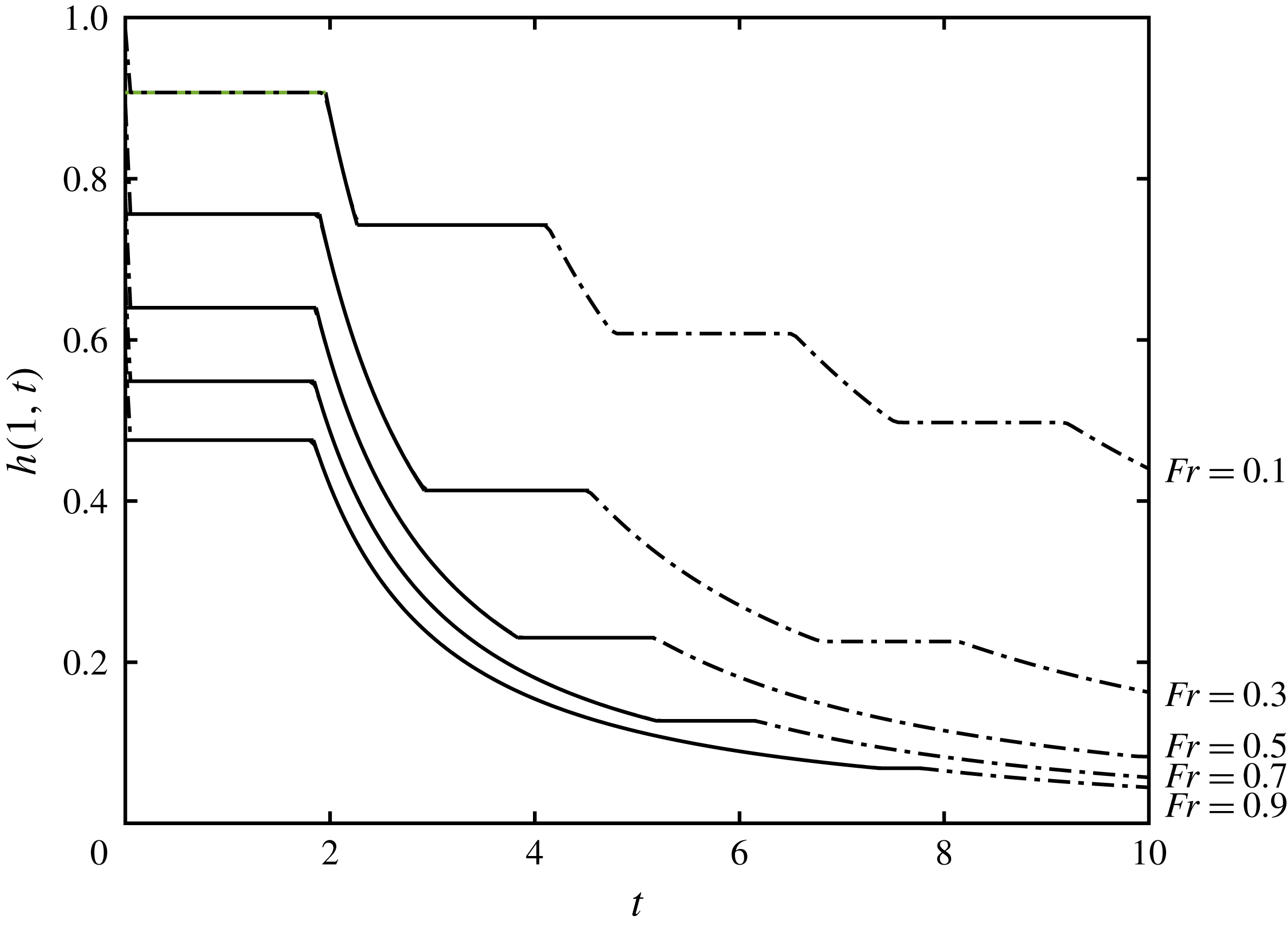
4.2 Long time evolution: similarity solution
After relatively long times, the flow evolves from its initial conditions to a state in which the motion is well captured by similarity solutions that are constructed below. These extend the solution developed by Momen et al. (Reference Momen, Zheng, Bou-Zeid and Stone2017) for an unconstricted outflow, in which the Froude number is unity, to a more general case where the Froude number is given by (4.1). As shown by Momen et al. (Reference Momen, Zheng, Bou-Zeid and Stone2017), for this class of similarity solution, the spatial coordinate,
 $x$
, is not geared to time and the height and velocity fields have the following form,
 $$\begin{eqnarray}h(x,t)=\frac{{\hat{H}}(x)}{t^{2}}\quad \text{and}\quad u(x,t)=\frac{\hat{U} (x)}{t},\end{eqnarray}$$
where
 ${\hat{H}}(x)$
and
 $\hat{U} (x)$
are to be determined. This dependence on
 $t$
is required in order to satisfy the drainage condition,
 $u(1,t)=Fr\sqrt{h(1,t)}$
, and to balance the terms in the momentum equation (2.1b
). On substitution into the governing equations (2.1a
) and (2.1b
), we find that
 $$\begin{eqnarray}\frac{\text{d}{\hat{H}}}{\text{d}x}=\frac{\hat{U} {\hat{H}}}{\hat{U} ^{2}-{\hat{H}}}\quad \text{and}\quad \frac{\text{d}\hat{U} }{\text{d}x}=\frac{\hat{U} ^{2}-2{\hat{H}}}{\hat{U} ^{2}-{\hat{H}}},\end{eqnarray}$$
together with the boundary conditions at the back wall and at the outflow, respectively given by
 $$\begin{eqnarray}\hat{U} (0)=0\quad \text{and}\quad \hat{U} (1)=Fr\sqrt{H_{1}},\end{eqnarray}$$
where
 $H_{1}={\hat{H}}(1)$
. We progress by introducing
 $\hat{V}=\hat{U} ^{2}/{\hat{H}}$
and then on the assumption that
 $\text{d}{\hat{H}}/\text{d}x$
does not vanish, we find that
 $$\begin{eqnarray}\frac{\text{d}\hat{V}}{\text{d}{\hat{H}}}=\frac{\hat{V}-4}{{\hat{H}}}.\end{eqnarray}$$
Integrating (4.7), and imposing
 ${\hat{H}}=H_{0}$
when
 $\hat{V}=\hat{U} =0$
at
 $x=0$
, we deduce that
 $$\begin{eqnarray}\hat{V}=4\left(1-\frac{{\hat{H}}}{H_{0}}\right).\end{eqnarray}$$
The latter boundary condition (4.6) demands that
 $\hat{V}=Fr^{2}$
when
 ${\hat{H}}=H_{1}$
at
 $x=1$
, and thus from (4.8), we find that
 $$\begin{eqnarray}\frac{H_{1}}{H_{0}}=1-\left(\frac{Fr}{2}\right)^{2}.\end{eqnarray}$$
To obtain
 ${\hat{H}}(x)$
we rewrite (4.8) in terms of
 $\hat{U}$
 $$\begin{eqnarray}\hat{U} =2\sqrt{{\hat{H}}}\sqrt{1-\frac{{\hat{H}}}{H_{0}}},\end{eqnarray}$$
and substitute into (4.5a ) to derive the implicit solution
 $$\begin{eqnarray}\frac{x}{\sqrt{H_{0}}}=-\frac{\unicode[STIX]{x03C0}}{2}+2\sqrt{\frac{{\hat{H}}}{H_{0}}}\sqrt{1-\frac{{\hat{H}}}{H_{0}}}+\arcsin \sqrt{\frac{{\hat{H}}}{H_{0}}}.\end{eqnarray}$$
The value of
 $H_{0}$
is found by setting
 $x=1$
and substituting (4.9) into the above equation, which yields
 $$\begin{eqnarray}H_{0}=\left(-\frac{\unicode[STIX]{x03C0}}{2}+Fr\sqrt{1-\left(\frac{Fr}{2}\right)^{2}}+\arccos \frac{Fr}{2}\right)^{-2}.\end{eqnarray}$$
The velocity field
 $\hat{U} (x)$
is found from (4.10). The solutions for various values of the Froude number are plotted in figure 12. We note that the fluid decreases in depth monotonically from the rear of the flow to the front. This generates a streamwise pressure gradient that accelerates the flow and drives the fluid through the constriction. Lower values of the Froude number, corresponding to smaller widths at the constriction, lead to reduced velocities and weaker pressure gradients.
The similarity functions (a)
 $H(x)-H_{1}$
and (b)
 $U(x)$
as a function of distance from the back wall,
 $x$
, for various Froude numbers at the constriction
 $(x=1)$
: (i)
 $Fr=0.1$
; (ii)
 $Fr=0.3$
; (iii)
 $Fr=0.5$
; (iv)
 $Fr=0.7$
; and (v)
 $Fr=0.9$
.

These similarity solutions are compared with the results from the numerical integration of the governing equations; in figure 13, we compare the numerically determined height at the outflow with the prediction from the similarity solution. In this study we have integrated numerically from lock-release initial conditions, which are evidently not in self-similar form of (4.4); thus we find that the similarity solutions is approached progressively. We also note that the self-similarity functions (4.4) are only defined up to an arbitrary origin in time; in other words, we could replace
 $t$
with
 $t-\hat{t}_{0}$
in (4.4) and the same solutions are maintained. Evidently at sufficiently long times,
 $t\gg |\hat{t}_{0}|$
, this makes negligible difference to the predictions of the similarity solutions, but at short times, we may select
 $\hat{t}_{0}$
to closely match the evolution from lock-release conditions at relatively short times. In figure 13 we have chosen
 $\hat{t}_{0}=-\sqrt{H_{1}}$
, so that the similarity solution predicts a height of unity at
 $x=1$
and
 $t=0$
and we note that this leads to a close correspondence with the numerically computed value (see figure 13). For relatively small values of the Froude number,
 $Fr$
, the magnitude of the temporal offset,
 $\hat{t}_{0}$
is quite large; its effect is that the long time, self-similar form in which
 $h(1,t)$
is proportional to
 $1/t^{2}$
is not realised until very late times (and in the case
 $Fr=0.1$
, beyond the computational range plotted in figure 13).
The height at the outflow,
 $h(1,t)$
, as a function of time for various values of the Froude number: (i)
 $F=0.1$
; (ii)
 $F=0.3$
; (iii)
 $F=0.5$
; (iv)
 $F=0.7$
; and (v)
 $F=0.9$
. The solid line plots the results from the numerical integration of the governing equations initiated with lock-release conditions and the dotted lines plot the similarity solution,
 $H_{1}/(t+\sqrt{H_{1}})^{2}$
.

The similarity solution captures the leading-order decay of the dependent variables. However it does not include the oscillations that occur as fluid sloshes between the back wall and the drainage boundary. These oscillations are manifest as intervals during which the height at the drainage boundary remains constant (figure 13). Interestingly, and in contrast to the draining flow over a barrier § 3, they appear not to have a fixed period, but rather the duration between them progressively increases. This observation will be studied in the next subsection.
4.3 Linear stability of similarity solution
We may analyse the progressive approach of the draining dynamics through a constriction to the similarity solution (4.4), by computing the linear stability of the latter. Following Grundy & Rottman (Reference Grundy and Rottman1985) and Mathunjwa & Hogg (Reference Mathunjwa and Hogg2006), we introduce a small perturbation to the solutions for the height and velocity fields, denoted by
 $\tilde{H}(x)$
and
 $\tilde{U} (x)$
respectively, so that
 $$\begin{eqnarray}h=\frac{{\hat{H}}(x)}{t^{2}}+\unicode[STIX]{x1D6FF}\frac{\tilde{H}(x)}{t^{\unicode[STIX]{x1D6FE}+2}}\quad \text{and}\quad u=\frac{\hat{U} (x)}{t}+\unicode[STIX]{x1D6FF}\frac{\tilde{U} (x)}{t^{\unicode[STIX]{x1D6FE}+1}},\end{eqnarray}$$
where
 $\unicode[STIX]{x1D6FF}$
is a small ordering parameter
 $(\unicode[STIX]{x1D6FF}\ll 1)$
and
 $\unicode[STIX]{x1D6FE}$
is to be determined. On substitution into the governing equations (2.1a
) and (2.1b
) and after linearisation, we find that
 $$\begin{eqnarray}\displaystyle & \displaystyle -(2+\unicode[STIX]{x1D6FE})\tilde{H}+\frac{\text{d}}{\text{d}x}\left(\tilde{H}\hat{U} +\tilde{U} {\hat{H}}\right)=0, & \displaystyle\end{eqnarray}$$
 $$\begin{eqnarray}\displaystyle & \displaystyle -(1+\unicode[STIX]{x1D6FE})\tilde{U} +\frac{\text{d}}{\text{d}x}\left(\tilde{U} \hat{U} +\tilde{H}\right)=0. & \displaystyle\end{eqnarray}$$
The boundary conditions represent no flow at the back wall,
 $\tilde{U} (0)=0$
, and the linearised drainage condition is given by
 $$\begin{eqnarray}2\hat{U} (1)\tilde{U} (1)=Fr^{2}\tilde{H}(1).\end{eqnarray}$$
Straightforwardly, we note that
 $\unicode[STIX]{x1D6FE}=1$
is a solution, with
 $\tilde{H}=2{\hat{H}}$
and
 $\tilde{U} =\hat{U}$
; this corresponds to the introduction of a shift of the temporal origin, which, as discussed above, does not change the similarity solution. In addition,
 $\unicode[STIX]{x1D6FE}=0$
is a solution with
 $\tilde{U} =\text{d}\hat{U} /\text{d}x$
and
 $\tilde{H}=\text{d}{\hat{H}}/\text{d}x$
; this corresponds to a translation of the
 $x$
-axis. Both of the these solutions are inevitably found in the study of the stability of similarity solutions and do not reveal the linear stability properties (Mathunjwa & Hogg Reference Mathunjwa and Hogg2006). Instead we seek non-trivial solutions to (4.14)–(4.15), which determine the exponent,
 $\unicode[STIX]{x1D6FE}$
, as an eigenvalue.
We determine the eigenvalue,
 $\unicode[STIX]{x1D6FE}$
, through numerical integration of (4.14)–(4.15), using the solution for
 ${\hat{H}}(x)$
and
 $\hat{U} (x)$
given by (4.10) and (4.11); in this computation, we allow the eigenvalue and functions to be complex valued, noting that since the governing equations have real-valued coefficients, they are also satisfied by the complex conjugates of the solutions. We plot the value of
 $\unicode[STIX]{x1D6FE}$
with the smallest real part in figure 14 as a function of the drainage Froude number,
 $Fr$
. We note that
 $\Re (\unicode[STIX]{x1D6FE})>0$
and thus the similarity solutions are linearly stable; in other words, all disturbances decay more rapidly than the solutions itself. In fact, we note that
 $\Re (\unicode[STIX]{x1D6FE})$
is only relatively weakly dependent upon
 $Fr$
. However the eigenvalue also has a non-vanishing imaginary part and its relatively strong variation is also plotted in figure 14.
The exponent,
 $\unicode[STIX]{x1D6FE}$
, as a function of the Froude number,
 $Fr$
.

We may use this solution to analyse the oscillations noted above in the numerically determined solution to the drainage from lock-release initial conditions (figure 13). Denoting the ratio between successive times at which the height at the end of the domain exhibits a spatially uniform region by
 ${\mathcal{R}}$
, we find that
 $$\begin{eqnarray}{\mathcal{R}}=\exp \left(\frac{2\unicode[STIX]{x03C0}}{\unicode[STIX]{x1D6FE}_{I}}\right),\end{eqnarray}$$
where
 $\unicode[STIX]{x1D6FE}_{I}\equiv \Im (\unicode[STIX]{x1D6FE})$
denotes the imaginary part of the exponent
 $\unicode[STIX]{x1D6FE}$
. In figure 15 we plot
 ${\mathcal{R}}$
as a function of the Froude number,
 $Fr$
; we observe that the ratio of successive periods increases monotonically with
 $Fr$
. We also examine this ratio in our numerical results by computing
 ${\mathcal{R}}_{n}=(t_{n}-t_{0})/(t_{n-1}-t_{0})$
, the ratio of the
 $n$
th to
 $(n-1)$
th times at which the period of a constant fluid depth at
 $x=1$
starts as a function of
 $n$
for
 $Fr=0.1$
and
 $Fr=0.5$
(see inset figures in figure 15). In both cases we find that the numerically determined ratio approaches the asymptotic prediction; initially there are differences because the motion is strongly nonlinear, but these diminish as the flow evolves into a state that is accurately represented by this linearised analysis. We note that for
 $Fr=0.1$
there are many oscillations observed during the computational period, because the ratio,
 ${\mathcal{R}}$
is quite close to unity. In contrast, when
 $Fr=0.5$
, the ratio of the successive oscillations is larger and so fewer can be determined in the numerical results before their amplitude has very substantially diminished.
The ratio of successive times at which the height at the outflow exhibits periods during which it is constant,
 ${\mathcal{R}}$
, as a function of the Froude number,
 $Fr$
. The inset figures show the numerically determined ratio,
 ${\mathcal{R}}_{n}$
, as a function of the oscillation number
 $n$
(shown with symbols) and the theoretical prediction (dashed line) for
 $Fr=0.1$
and
 $Fr=0.5$
.

5 Summary and conclusions
The fluid mechanics of the gravitationally driven drainage of an initially quiescent reservoir following the partial removal of its confining dam have been investigated in detail using the shallow water equations to reveal the temporal and spatial dependencies of the depth and velocity of the flowing layer. For scenarios in which the reservoir drains over a barrier and through a constriction, we have shown how the unsteady motion evolves towards a state in which there is progressive drainage and relatively rapid wave motions that run between the back wall of the reservoir and the partially removed dam. When the fluid drains over a weir (a partially removed dam that leaves a barrier of height
 $D$
), we find that after sufficient time following the flow initiation, the excess height diminishes in proportion to
 $t^{-2}$
, while the velocity at the overflow varies as
 $t^{-3}$
. Relatively fast moving waves propagate between the outflow and back wall of the reservoir with dimensionless phase speed,
 $\sqrt{D}$
and amplitude that diminishes as
 $t^{-3}$
. In contrast when the flow is through a constriction alone (
 $D=0$
and
 $w<1$
), the height of the fluid layer also decreases as
 $t^{-2}$
, but the velocity is proportional to
 $t^{-1}$
. The motion in this scenario becomes self-similar to leading order after sufficient time has elapsed following initiation. Wave-like disturbances emerge, but their wave speed diminishes exponentially in time and in relation to the width of the constricted outflow.
The results have been determined using three approaches, each of which has necessitated some innovations. First we have used the hodograph transformation to convert the governing nonlinear partial differential equations to a linear system that may be tackled using analytical techniques. The solutions are given by quasi-analytical expressions and are evaluated though numerical quadrature to reveal the initial gravitational slumping and the onset of the oscillatory behaviour. In principle these calculations could be extended to much later times, although the oscillations entail rather tedious analytical bookkeeping. Direct numerical integration of the governing equations provide solutions as well and we have employed a numerical method that carefully imposes the boundary conditions at the outflow, while minimising internal numerical dissipation, so that features with discontinuous gradients of the dependent variables can be captured accurately. The numerical results, validated by the analytical results obtained through hodograph techniques, may be extended to late times to reveal the progressive drainage and the oscillations that manifest themselves as intervals during which the height and velocity of the fluid layer adjacent to the back wall or the outflow are spatially uniform. The oscillations persist although their amplitude diminishes. At late times for flows over a barrier, we have employed a multiple time-scale asymptotic technique to determine the draining and wave-like motions. The algebraic details of this asymptotic result are somewhat cumbersome given that the amplitude and phase are only established by calculating to relatively high order and using repeated secular conditions to ensure uniformity of the asymptotic expansion, but the results compactly reveal the oscillations within the reservoir. Furthermore the asymptotic solutions confirm the accuracy of the numerical computations at late times. In contrast, flows through constrictions approach a self-similar state at late times, in which the oscillations can be interpreted as the linear stability of this state. We showed that the direct prediction of the exponential growth of the period of the oscillations was realised by the numerical computations. The result and interpretation have bearings on other inertially dominated, self-similar flows, such as gravity current dynamics from lock-release initial conditions.
The unsteady fluid mechanics of this study may have important consequences for the draining of natural-scale reservoirs following the partial removal of their containing dam. The calculations show that the volume flux of fluid per unit width leaving the reservoir diminishes temporally and at late times is proportional to
 $t^{-3}$
for both flows over weirs and through constrictions. It would be interesting to test this and other predictions from our analysis against laboratory or large-scale observations. The problem is also a useful test-bed solution for numerical integration of either the shallow-water equations, for which we have established a non-trivial analytical solution at both early and late times or for other simulations of fluid flow in this configuration. For example, the OpenFoam library for the direct numerical simulation of the Navier–Stokes equations identifies unsteady reservoir draining as an important trial problem and Momen et al. (Reference Momen, Zheng, Bou-Zeid and Stone2017) used this computational library to simulate flow over an edge
 $(D=0,w=1)$
; it would be also interesting to simulate flows for the more general problem analysed in this study. There are also several extensions to flows in related configurations that would be interesting to pursue. For example, how does the dynamics differ if the reservoir gravitationally slumps and flows towards a distant barrier, which it may overtop? Furthermore in the Boussinesq regime, how are the interactions modified if the impinging fluid is able to mix with its surroundings? Some aspects of this type of motion have been considered by Nabi & Flynn (Reference Nabi and Flynn2013), in which they model and confirm through experiments the mixing downstream of a weir. We anticipate that some of our new methodologies and results may be adapted to these new scenarios.
Acknowledgements
E.W.G.S. acknowledges the support of an EPSRC (UK) studentship and A.J.H. acknowledges the support of the Royal Society (APX\R1\180148).
Appendix A. Derivation of the outflow boundary condition
The outflow boundary condition at
 $x=1$
can be found in textbooks such as Ackers et al. (Reference Ackers, White, Perkins and Harrison1978) and Dake (Reference Dake1983), and is derived using classical hydrodynamic principles for inviscid flows. In particular for a steady state, the mass flux is constant and energy is conserved in regions where the flow varies continuously i.e. away from hydraulic jumps. Moreover as the fluid flows over a smooth barrier, or through a smooth constriction, it may accelerate from a subcritical state to a supercritical state and is therefore critical at some interior location.
The geometry of the barrier or constriction at the outflow is such that the variation in the width of the channel or the elevation of the bed induces non-negligible lateral and vertical velocities only over
 $1-\hat{\unicode[STIX]{x1D716}}<x<1$
, where
 $\hat{\unicode[STIX]{x1D716}}\ll 1$
is a relatively small dimensionless length, whereas over the bulk of the interior
 $(0\leqslant x\leqslant 1-\hat{\unicode[STIX]{x1D716}})$
, the bed elevation and width are constant and the flow is aligned with the
 $x$
-axis. We denote the width of the channel relative to the uniform width in the bulk by
 ${\hat{w}}(x)$
, noting that
 ${\hat{w}}(1)=w$
at the narrowest part of the outflow. Likewise we denote the bed elevation by
 $\hat{D}(x)$
, non-dimensionalised with respect to the initial depth of the reservoir and note that
 $\hat{D}(1)=D$
. We may then extend our shallow water equations to include width variations; the governing equations (2.1a
) and (2.1b
) are then given by the dimensionless Saint-Venant equations (Chow Reference Chow2009)
 $$\begin{eqnarray}\frac{\unicode[STIX]{x2202}}{\unicode[STIX]{x2202}t}({\hat{w}}h)+\frac{\unicode[STIX]{x2202}}{\unicode[STIX]{x2202}x}(u{\hat{w}}h)=0,\quad \frac{\unicode[STIX]{x2202}u}{\unicode[STIX]{x2202}t}+\frac{\unicode[STIX]{x2202}}{\unicode[STIX]{x2202}x}\left(\frac{u^{2}}{2}+h+\hat{D}\right)=0.\end{eqnarray}$$
Respectively these represent the width- and depth-averaged expressions of the conservation of mass and the balance of streamwise momentum on the assumption that the contraction in width is much less than the streamwise extent of the reservoir
 $(W(1-w)/L\ll 1)$
so that the lateral velocities remain relatively small. We note that away from the outflow
 $0\leqslant x\leqslant 1-\hat{\unicode[STIX]{x1D716}}$
,
 ${\hat{w}}=1$
and
 $\hat{D}=0$
and the governing equations reduce to (2.1a
) and (2.1b
). Furthermore the dimensionless extent of the upstream distance over which the barrier or constriction influences the flow is estimated to be the greater of the ratio of the barrier height to the streamwise length scale, or the constricted width to the streamwise length scale, both of which are assumed to be small. The solutions within the region adjacent to the outflow
 $(1-\hat{\unicode[STIX]{x1D716}}<x<1)$
evolve on very short time scales of
 $O(\hat{\unicode[STIX]{x1D716}})$
, because this is the time scale over which characteristics cross the domain. Conversely within the bulk of the domain, the flow evolves on time scales of order unity. Therefore, for the purpose of modelling the flow in the bulk we may consider the flow local to the boundary to be in a quasi-steady state. In what follows we derive an outflow boundary condition that applies to the flow at
 $x=1-\hat{\unicode[STIX]{x1D716}}$
, namely at the upstream location where the channel width and bed elevation induce non-streamwise velocities.
The steady states of the Saint-Venant equations are given by
 $$\begin{eqnarray}u{\hat{w}}h=q,\quad \frac{u^{2}}{2}+h+\hat{D}=E,\end{eqnarray}$$
for some
 $q$
and
 $E$
, which represent the dimensionless volume flux and energy, respectively. The Saint-Venant equations provide a model for the evolution of a channel-averaged velocity; if, instead a three-dimensional velocity field had been modelled using the inviscid Euler equation, then (A 2b
) with
 $u^{2}$
replaced by
 $|\boldsymbol{u}|^{2}$
would represent the application of Bernoulli’s theorem on the surface streamline. In what follows we relate the flow conditions at the location where the motion begins to deviate from purely horizontal flow aligned with the
 $x$
-axis
 $(x=1-\hat{\unicode[STIX]{x1D716}})$
to conditions at the highest and narrowest point of the barrier
 $(x=1)$
, at which position we assume that the flow is also only horizontal and aligned with the
 $x$
-axis. Thus energy conservation between these two locations is given by (A 2b
). We assume that the inflow at
 $x=1-\hat{\unicode[STIX]{x1D716}}$
is subcritical (slow and deep), and that in
 $x>1$
the bed slopes downward and the channel widens so that the fluid becomes supercritical (fast and shallow). At
 $x=1$
,
 $E-D(x)$
is minimised and consequentially so is
 $u^{2}/2+h$
. Thus the flow is critical at the outflow
 $x=1$
, and we may write
 $u_{out}=\sqrt{h_{out}}$
. Then by conservation of volume flux (A 2)
 $$\begin{eqnarray}h_{out}=\left(\frac{q}{w}\right)^{2/3},\end{eqnarray}$$
which yields the expression for the energy
 $$\begin{eqnarray}E=\frac{3}{2}\left(\frac{q}{w}\right)^{2/3}+D.\end{eqnarray}$$
We construct the boundary condition for the bulk at
 $x=1-\hat{\unicode[STIX]{x1D716}}$
using conservation of energy (A 2b
)
 $$\begin{eqnarray}\left.\frac{u^{2}}{2}+h\right|_{x=1-\hat{\unicode[STIX]{x1D716}}}=\frac{3}{2}\left(\frac{q}{w}\right)^{2/3}+D,\quad \text{where }q=wu_{out}h_{out}=uh|_{x=1-\hat{\unicode[STIX]{x1D716}}}.\end{eqnarray}$$
Finally, limiting
 $\hat{\unicode[STIX]{x1D716}}\rightarrow 0$
yields the boundary condition
 $$\begin{eqnarray}u^{2}+2(h-D)-3\left(\frac{uh}{w}\right)^{2/3}=0\quad \text{at }x=1.\end{eqnarray}$$
The modelling framework in this appendix and in § 2 is built upon the assumption that the depth of the fluid layer is much smaller than any streamwise or lateral length scale so that the pressure adopts a hydrostatic distribution. Deviations from this hierarchy of length scales could lead to head loss (dissipation) which is not included in the current description. If we assume that the energy dissipation is of magnitude
 $\unicode[STIX]{x0394}E$
between the bulk and the outflow, then we have the condition
 $$\begin{eqnarray}\left.u^{2}+2(h-D)-3\left(\frac{uh}{w}\right)^{2/3}\right|_{x=1}=2\unicode[STIX]{x0394}E.\end{eqnarray}$$
The energy loss,
 $\unicode[STIX]{x0394}E$
, has been evaluated empirically. Following Zachoval et al. (Reference Zachoval, Knéblová, Rous̆ar, Rumann and S̆ulc2014), we introduce a discharge coefficient
 $C_{d}$
given by
 $$\begin{eqnarray}uh=\left(\frac{2}{3}\right)^{3/2}C_{d}w\left(\frac{u^{2}}{2}+h-D\right)^{3/2}.\end{eqnarray}$$
This means that the discharge coefficient measures the energy ratio between the critical outflow and the bulk, where the depths are measured relative to the bed elevation at the outflow, i.e.
 $$\begin{eqnarray}C_{d}^{2/3}=\left.\left[\frac{3}{2}\left(\frac{uh}{w}\right)^{2/3}\right]/\left[\frac{u^{2}}{2}+h-D\right]\right|_{x=1}.\end{eqnarray}$$
Note that the numerator in this expression is the energy at the outflow, despite being evaluated at the bottom of the slope, because the critical energy is only dependent on the volume flux (which is conserved between the bottom and top of the slope) and the width of the channel. It is clear from (A 9) that for energy conserving flows
 $C_{d}=1$
. Rearranging (A 9) using (A 7) we obtain
 $$\begin{eqnarray}\unicode[STIX]{x0394}E=\frac{3}{2}\left(\frac{1}{C_{d}^{2/3}}-1\right)\left(\frac{uh}{w}\right)^{2/3}.\end{eqnarray}$$
Thus we can write the boundary condition in terms of the discharge coefficient
 $$\begin{eqnarray}\left.u^{2}+2(h-D)-3\left(\frac{uh}{C_{d}w}\right)^{2/3}\right|_{x=1}=0.\end{eqnarray}$$
From the results in Zachoval et al. (Reference Zachoval, Knéblová, Rous̆ar, Rumann and S̆ulc2014), we find that
 $0.83\lesssim C_{d}\lesssim 0.95$
, which gives us
 $$\begin{eqnarray}1.03\lesssim \frac{1}{C_{d}^{2/3}}\lesssim 1.13.\end{eqnarray}$$
On this basis we conclude that the effect of dissipation can be neglected to a good approximation. Even if it cannot be ignored then we can simply include it in our model by modifying the definition of
 $w$
to be the drainage coefficient multiplied by the ratio of outflow width to channel width.
Explicit account of viscous processes has been ignored in this analysis and potentially at late times, when the flow is very thin at the crest of the barrier, viscous stresses could play a dynamical role. To this end we assess when the dimensional inertial terms of the governing equations,
 $u\unicode[STIX]{x2202}u/\unicode[STIX]{x2202}x$
, become comparable with the (currently omitted) dimensional viscous terms,
 $\unicode[STIX]{x1D708}\unicode[STIX]{x2202}^{2}u/\unicode[STIX]{x2202}z^{2}$
, where
 $\unicode[STIX]{x1D708}$
is the kinematic viscosity. The viscous stresses are largest where the flow is shallowest at the crest of the barrier, at which location the relevant streamwise dimensional length scale is
 $\hat{\unicode[STIX]{x1D716}}L$
. Viscous terms therefore become non-negligible when the reduced Reynolds number,
 $Re\equiv {\mathcal{U}}{\mathcal{H}}^{2}/(\unicode[STIX]{x1D708}\hat{\unicode[STIX]{x1D716}}L)$
, is order unity, where
 ${\mathcal{U}}$
and
 ${\mathcal{H}}$
are dimensional estimates of the velocity and height fields. Inserting our dimensionless expressions for the velocity and height at the outflow when the height of the fluid layer is comparable with the maximum barrier height, we find that
 $$\begin{eqnarray}Re=\frac{(g^{\prime }H^{5})^{1/2}}{\hat{\unicode[STIX]{x1D716}}L\unicode[STIX]{x1D708}}(h-D)^{5/2},\end{eqnarray}$$
where the reduced gravity is denoted by
 $g^{\prime }=\unicode[STIX]{x0394}\unicode[STIX]{x1D70C}g/\unicode[STIX]{x1D70C}$
and
 $h$
and
 $D$
are the dimensionless height of the fluid layer at the outflow of the domain and the barrier height, respectively. For free-surface flow of water
 $g^{\prime }\sim 10~\text{m}~\text{s}^{-2}$
and
 $\unicode[STIX]{x1D708}\sim 10^{-6}~\text{m}^{2}~\text{s}^{-1}$
. Then for a release of scale height
 $H\sim 10~\text{m}$
and a barrier of streamwise length scale
 $\hat{\unicode[STIX]{x1D716}}L\sim 100~\text{m}$
, we find that the reduced Reynolds number becomes of order unity when
 $h-D\sim 10^{-3}$
. Thus for these parameter values, the neglect of boundary viscous shear stress is also reasonable until
 $h-D\sim 10^{-3}$
. Conversely at laboratory scales,
 $H\sim 10~\text{cm}$
and
 $\hat{\unicode[STIX]{x1D716}}L\sim 1~\text{cm}$
, we find that that viscous effects are negligible until
 $h-D\sim 4\times 10^{-2}$
.
Appendix B. Computation of the asymptotic solution
B.1 Bounded waves with resonant forcing
In order to construct the wave components in the multi-scale expansion of § 3.3 we need to bound the terms in the expansions, producing solvability conditions that eliminate the secular terms. As we show in the following subsection, the possibility of secular terms comes from the existence of resonant forcing in the linearised wave equations. Our analysis often encounters a forced linear wave equation to which we apply homogeneous boundary conditions. Therefore we first present a general result that enables the construction of bounded solutions.
Theorem 1. Let
 $F_{L},F_{R},G_{L},G_{R}:\mathbb{R}\rightarrow \mathbb{R}$
be such that the derivatives
 $F_{L}^{\prime }$
,
 $F_{R}^{\prime }$
,
 $G_{L}^{\prime \prime }$
,
 $G_{R}^{\prime \prime }$
have period
 $2$
. The solution
 $u(x,t)$
to the forced linear wave equation
 $$\begin{eqnarray}\frac{1}{4c^{2}}\left[\frac{\unicode[STIX]{x2202}^{2}u}{\unicode[STIX]{x2202}t^{2}}-c^{2}\frac{\unicode[STIX]{x2202}^{2}u}{\unicode[STIX]{x2202}x^{2}}\right]=F_{L}^{\prime }(ct+x)+F_{R}^{\prime }(ct-x)+2x[G_{L}^{\prime \prime }(ct+x)+G_{R}^{\prime \prime }(ct-x)],\end{eqnarray}$$
on
 $x\in [0,1]$
with homogeneous Dirichlet boundary conditions
 $u(0,t)=u(1,t)=0$
is bounded if and only if
 $$\begin{eqnarray}\displaystyle & \displaystyle F_{R}(y)-F_{L}(y)+G_{R}(y)+G_{L}(y)+G_{R}^{\prime }(y)-G_{L}^{\prime }(y)=0, & \displaystyle\end{eqnarray}$$
 $$\begin{eqnarray}\displaystyle & \displaystyle F_{R}(y+2)-F_{R}(y)=-[G_{R}(y+2)-G_{R}(y)], & \displaystyle\end{eqnarray}$$
 $$\begin{eqnarray}\displaystyle & \displaystyle F_{L}(y+2)-F_{L}(y)=G_{L}(y+2)-G_{R}(y), & \displaystyle\end{eqnarray}$$
 $$\begin{eqnarray}\displaystyle & \displaystyle G_{R}^{\prime }(y+2)-G_{R}^{\prime }(y)=0, & \displaystyle\end{eqnarray}$$
 $$\begin{eqnarray}\displaystyle & \displaystyle G_{L}^{\prime }(y+2)-G_{L}^{\prime }(y)=0, & \displaystyle\end{eqnarray}$$
 $u$
is bounded on some
 $(x,t)\in [0,1]\otimes [t_{0},t_{0}+2/c)$
. Moreover, the solution can be expressed as
 $$\begin{eqnarray}\displaystyle u(x,t) & = & \displaystyle f(ct-x)-f(ct+x)+2x[F_{R}(ct-x)+G_{R}(ct-x)-F_{L}(ct+x)+G_{L}(ct+x)]\nonumber\\ \displaystyle & & \displaystyle +\,2x^{2}[G_{R}(ct-x)-G_{L}(ct+x)],\end{eqnarray}$$
where
 $f$
is an arbitrary period
 $2$
function.
Proof. We begin by simplifying the wave equation to the canonical form by making the change of variables
 $\unicode[STIX]{x1D709}=ct+x$
,
 $\unicode[STIX]{x1D702}=ct-x$
, and defining
 $U(\unicode[STIX]{x1D709},\unicode[STIX]{x1D702})=u((\unicode[STIX]{x1D709}-\unicode[STIX]{x1D702})/2,(\unicode[STIX]{x1D709}+\unicode[STIX]{x1D702})/2c)$
, resulting in
 $$\begin{eqnarray}\frac{\unicode[STIX]{x2202}^{2}U}{\unicode[STIX]{x2202}\unicode[STIX]{x1D709}\unicode[STIX]{x2202}\unicode[STIX]{x1D702}}=F_{L}^{\prime }(\unicode[STIX]{x1D709})+F_{R}^{\prime }(\unicode[STIX]{x1D702})+(\unicode[STIX]{x1D709}-\unicode[STIX]{x1D702})[G_{L}^{\prime \prime }(\unicode[STIX]{x1D709})+G_{R}^{\prime \prime }(\unicode[STIX]{x1D702})],\end{eqnarray}$$
which can be integrated to produce the general solution
 $$\begin{eqnarray}\displaystyle U & = & \displaystyle \hat{f}(\unicode[STIX]{x1D702})+{\hat{g}}(\unicode[STIX]{x1D709})+\unicode[STIX]{x1D702}F_{L}(\unicode[STIX]{x1D709})+\unicode[STIX]{x1D709}F_{R}(\unicode[STIX]{x1D702})-\unicode[STIX]{x1D702}G_{L}(\unicode[STIX]{x1D709})+\unicode[STIX]{x1D709}G_{R}(\unicode[STIX]{x1D702})\nonumber\\ \displaystyle & & \displaystyle +\,\left(\unicode[STIX]{x1D709}\unicode[STIX]{x1D702}-\frac{\unicode[STIX]{x1D702}^{2}}{2}\right)G_{L}^{\prime }(\unicode[STIX]{x1D709})-\left(\unicode[STIX]{x1D709}\unicode[STIX]{x1D702}-\frac{\unicode[STIX]{x1D709}^{2}}{2}\right)G_{R}^{\prime }(\unicode[STIX]{x1D702}),\end{eqnarray}$$
where
 $\hat{f}$
and
 ${\hat{g}}$
are the arbitrary functions of integration. Imposing the boundary conditions
 $U=0$
on
 $\unicode[STIX]{x1D702}=\unicode[STIX]{x1D709}$
and
 $\unicode[STIX]{x1D709}=\unicode[STIX]{x1D702}+2$
yields
 $$\begin{eqnarray}{\hat{g}}(\unicode[STIX]{x1D709})=-\hat{f}(\unicode[STIX]{x1D709})-\unicode[STIX]{x1D709}(F_{L}(\unicode[STIX]{x1D709})+F_{R}(\unicode[STIX]{x1D709})-G_{L}(\unicode[STIX]{x1D709})+G_{R}(\unicode[STIX]{x1D709}))-\frac{\unicode[STIX]{x1D709}^{2}}{2}(G_{L}^{\prime }(\unicode[STIX]{x1D709})-G_{R}^{\prime }(\unicode[STIX]{x1D709})),\end{eqnarray}$$
 $$\begin{eqnarray}\displaystyle \hat{f}(\unicode[STIX]{x1D702}+2) & = & \displaystyle \hat{f}(\unicode[STIX]{x1D702})-2F_{L}(\unicode[STIX]{x1D702}+2)+(\unicode[STIX]{x1D702}+2)(F_{R}(\unicode[STIX]{x1D702})-F_{R}(\unicode[STIX]{x1D702}+2))\nonumber\\ \displaystyle & & \displaystyle +\,2G_{L}(\unicode[STIX]{x1D702}+2)+(\unicode[STIX]{x1D702}+2)(G_{R}(\unicode[STIX]{x1D702})-G_{R}(\unicode[STIX]{x1D702}+2))\nonumber\\ \displaystyle & & \displaystyle -\,2G_{L}^{\prime }(\unicode[STIX]{x1D702}+2)+\left(2-\frac{\unicode[STIX]{x1D702}^{2}}{2}\right)G_{R}^{\prime }(\unicode[STIX]{x1D702})+\frac{(\unicode[STIX]{x1D702}+2)^{2}}{2}G_{R}^{\prime }(\unicode[STIX]{x1D702}+2),\end{eqnarray}$$
 $$\begin{eqnarray}\displaystyle & & \displaystyle u(x,t+2/c)-u(x,t)=U(\unicode[STIX]{x1D709}+2,\unicode[STIX]{x1D702}+2)-U(\unicode[STIX]{x1D709},\unicode[STIX]{x1D702})\nonumber\\ \displaystyle & & \displaystyle \quad =2[F_{L}(\unicode[STIX]{x1D709}+2)-F_{R}(\unicode[STIX]{x1D709})-G_{L}(\unicode[STIX]{x1D709}+2)-G_{R}(\unicode[STIX]{x1D709})+G_{L}^{\prime }(\unicode[STIX]{x1D709}+2)-G_{R}^{\prime }(\unicode[STIX]{x1D709})]\nonumber\\ \displaystyle & & \displaystyle \qquad -\,2[F_{L}(\unicode[STIX]{x1D702}+2)-F_{R}(\unicode[STIX]{x1D702})-G_{L}(\unicode[STIX]{x1D702}+2)-G_{R}(\unicode[STIX]{x1D702})+G_{L}^{\prime }(\unicode[STIX]{x1D702}+2)-G_{R}^{\prime }(\unicode[STIX]{x1D702})]\nonumber\\ \displaystyle & & \displaystyle \qquad +\,(\unicode[STIX]{x1D709}-\unicode[STIX]{x1D702})[F_{L}(\unicode[STIX]{x1D709})-F_{L}(\unicode[STIX]{x1D709}+2)-G_{L}(\unicode[STIX]{x1D709})+G_{L}(\unicode[STIX]{x1D709}+2)]\nonumber\\ \displaystyle & & \displaystyle \qquad -\,(\unicode[STIX]{x1D709}-\unicode[STIX]{x1D702})[F_{R}(\unicode[STIX]{x1D702})-F_{R}(\unicode[STIX]{x1D702}+2)+G_{R}(\unicode[STIX]{x1D702})-G_{R}(\unicode[STIX]{x1D702}+2)]\nonumber\\ \displaystyle & & \displaystyle \qquad +\,\frac{(\unicode[STIX]{x1D709}-\unicode[STIX]{x1D702})^{2}}{2}[G_{L}^{\prime }(\unicode[STIX]{x1D709})-G_{L}^{\prime }(\unicode[STIX]{x1D709}+2)]-\frac{(\unicode[STIX]{x1D709}-\unicode[STIX]{x1D702})^{2}}{2}[G_{R}^{\prime }(\unicode[STIX]{x1D709})-G_{R}^{\prime }(\unicode[STIX]{x1D709}+2)].\end{eqnarray}$$
From here the conditions (B 2) follow. To deduce the form of the general solution (B 3) we make the substitution
 $$\begin{eqnarray}f(y)=\hat{f}(y)+y(F_{L}(y)-G_{L}(y)+G_{L}^{\prime }(y)-G_{R}^{\prime }(y))-\frac{y^{2}}{2}G_{R}^{\prime }(y),\end{eqnarray}$$
so that (B 6b
) enforces
 $f(y+2)=f(y)$
, and then substitute (B 6a
) into (B 5) and simplify using (B 2).☐
B.2 Expansion with multiple time scales
We expand the depth and velocity as sequences of undetermined functions dependent on the time scales (3.24)
 $$\begin{eqnarray}\displaystyle & \displaystyle h(x,t)-D=\unicode[STIX]{x1D716}^{2}h_{2}(x,T_{0},T_{1})+\unicode[STIX]{x1D716}^{3}h_{3}(x,T_{0},T_{1})+\cdots \,, & \displaystyle\end{eqnarray}$$
 $$\begin{eqnarray}\displaystyle & \displaystyle u(x,t)=\unicode[STIX]{x1D716}^{3}u_{3}(x,T_{0},T_{1})+\unicode[STIX]{x1D716}^{4}u_{4}(x,T_{0},T_{1})+\cdots \,, & \displaystyle\end{eqnarray}$$
 $h_{m}$
and
 $u_{m}$
are of order unity so that this is a uniform expansion. Substituting our expansions into the governing equations we obtain
 $$\begin{eqnarray}\displaystyle 0 & = & \displaystyle \frac{\unicode[STIX]{x2202}h}{\unicode[STIX]{x2202}t}+\frac{\unicode[STIX]{x2202}(uh)}{\unicode[STIX]{x2202}x}\end{eqnarray}$$
 $$\begin{eqnarray}\displaystyle & = & \displaystyle \unicode[STIX]{x1D716}^{2}\frac{\text{d}\unicode[STIX]{x1D714}_{0}}{\text{d}T_{1}}\frac{\unicode[STIX]{x2202}h_{2}}{\unicode[STIX]{x2202}T_{0}}+\unicode[STIX]{x1D716}^{3}\left[\frac{\text{d}\unicode[STIX]{x1D714}_{0}}{\text{d}T_{1}}\frac{\unicode[STIX]{x2202}h_{3}}{\unicode[STIX]{x2202}T_{0}}+\frac{\unicode[STIX]{x2202}h_{2}}{\unicode[STIX]{x2202}T_{1}}+D\frac{\unicode[STIX]{x2202}u_{3}}{\unicode[STIX]{x2202}x}\right]\nonumber\\ \displaystyle & & \displaystyle +\,\unicode[STIX]{x1D716}^{4}\left[\frac{\text{d}\unicode[STIX]{x1D714}_{0}}{\text{d}T_{1}}\frac{\unicode[STIX]{x2202}h_{4}}{\unicode[STIX]{x2202}T_{0}}+\frac{\unicode[STIX]{x2202}h_{3}}{\unicode[STIX]{x2202}T_{1}}+\frac{\text{d}\unicode[STIX]{x1D714}_{2}}{\text{d}T_{1}}\frac{\unicode[STIX]{x2202}h_{2}}{\unicode[STIX]{x2202}T_{0}}+D\frac{\unicode[STIX]{x2202}u_{4}}{\unicode[STIX]{x2202}x}\right]\nonumber\\ \displaystyle & & \displaystyle +\,\unicode[STIX]{x1D716}^{5}\left[\frac{\text{d}\unicode[STIX]{x1D714}_{0}}{\text{d}T_{1}}\frac{\unicode[STIX]{x2202}h_{5}}{\unicode[STIX]{x2202}T_{0}}+\frac{\unicode[STIX]{x2202}h_{4}}{\unicode[STIX]{x2202}T_{1}}+\frac{\text{d}\unicode[STIX]{x1D714}_{2}}{\text{d}T_{1}}\frac{\unicode[STIX]{x2202}h_{3}}{\unicode[STIX]{x2202}T_{0}}+\frac{\text{d}\unicode[STIX]{x1D714}_{3}}{\text{d}T_{1}}\frac{\unicode[STIX]{x2202}h_{2}}{\unicode[STIX]{x2202}T_{0}}+D\frac{\unicode[STIX]{x2202}u_{5}}{\unicode[STIX]{x2202}x}+\frac{\unicode[STIX]{x2202}(u_{3}h_{2})}{\unicode[STIX]{x2202}x}\right]+O(\unicode[STIX]{x1D716}^{6}),\nonumber\\ \displaystyle & & \displaystyle\end{eqnarray}$$
 $$\begin{eqnarray}\displaystyle 0 & = & \displaystyle \frac{1}{D}\left(\frac{\unicode[STIX]{x2202}(uh)}{\unicode[STIX]{x2202}t}+\frac{\unicode[STIX]{x2202}(u^{2}h)}{\unicode[STIX]{x2202}x}+h\frac{\unicode[STIX]{x2202}h}{\unicode[STIX]{x2202}x}\right)\end{eqnarray}$$
 $$\begin{eqnarray}\displaystyle & = & \displaystyle \unicode[STIX]{x1D716}^{2}\frac{\unicode[STIX]{x2202}h_{2}}{\unicode[STIX]{x2202}x}+\unicode[STIX]{x1D716}^{3}\left[\frac{\text{d}\unicode[STIX]{x1D714}_{0}}{\text{d}T_{1}}\frac{\unicode[STIX]{x2202}u_{3}}{\unicode[STIX]{x2202}T_{0}}+\frac{\unicode[STIX]{x2202}h_{3}}{\unicode[STIX]{x2202}x}\right]+\unicode[STIX]{x1D716}^{4}\left[\frac{\text{d}\unicode[STIX]{x1D714}_{0}}{\text{d}T_{1}}\frac{\unicode[STIX]{x2202}u_{4}}{\unicode[STIX]{x2202}T_{0}}+\frac{\unicode[STIX]{x2202}u_{3}}{\unicode[STIX]{x2202}T_{1}}+\frac{\unicode[STIX]{x2202}h_{4}}{\unicode[STIX]{x2202}x}+\frac{h_{2}}{D}\frac{\unicode[STIX]{x2202}h_{2}}{\unicode[STIX]{x2202}x}\right]\nonumber\\ \displaystyle & & \displaystyle +\,\unicode[STIX]{x1D716}^{5}\left[\frac{\text{d}\unicode[STIX]{x1D714}_{0}}{\text{d}T_{1}}\frac{\unicode[STIX]{x2202}u_{5}}{\unicode[STIX]{x2202}T_{0}}+\frac{\unicode[STIX]{x2202}u_{4}}{\unicode[STIX]{x2202}T_{1}}+\frac{\text{d}\unicode[STIX]{x1D714}_{2}}{\text{d}T_{1}}\frac{\unicode[STIX]{x2202}u_{3}}{\unicode[STIX]{x2202}T_{0}}+\frac{1}{D}\frac{\text{d}\unicode[STIX]{x1D714}_{0}}{\text{d}T_{1}}\frac{\unicode[STIX]{x2202}(u_{3}h_{2})}{\unicode[STIX]{x2202}T_{0}}+\frac{\unicode[STIX]{x2202}h_{5}}{\unicode[STIX]{x2202}x}+\frac{1}{D}\frac{\unicode[STIX]{x2202}\left(h_{2}h_{3}\right)}{\unicode[STIX]{x2202}x}\right]+O(\unicode[STIX]{x1D716}^{6}).\nonumber\\ \displaystyle & & \displaystyle\end{eqnarray}$$
The boundary condition at the rear of the lock demands that
 $u_{m}$
vanishes at
 $x=0$
, while the boundary condition at
 $x=1$
yields
 $$\begin{eqnarray}\displaystyle 0 & = & \displaystyle \frac{u^{2}}{2}+(h-D)-\frac{3}{2}\left(\frac{uh}{w}\right)^{2/3}\end{eqnarray}$$
 $$\begin{eqnarray}\displaystyle & = & \displaystyle \unicode[STIX]{x1D716}^{2}\left[h_{2}-\frac{3}{2}\left(\frac{Du_{3}}{w}\right)^{2/3}\right]+\unicode[STIX]{x1D716}^{3}\left[h_{3}-\left(\frac{Du_{3}}{w}\right)^{2/3}\frac{u_{4}}{u_{3}}\right]\nonumber\\ \displaystyle & & \displaystyle +\,\unicode[STIX]{x1D716}^{4}\left[h_{4}-\left(\frac{Du_{3}}{w}\right)^{2/3}\left(\frac{u_{5}}{u_{3}}+\frac{h_{2}}{D}-\frac{u_{4}^{2}}{6u_{3}^{2}}\right)\right]+O(\unicode[STIX]{x1D716}^{5}).\end{eqnarray}$$
We observe that the governing equations at
 $O(\unicode[STIX]{x1D716}^{2})$
give
 $h_{2}\equiv h_{2}(T_{1})$
. The balances at higher order will result in inhomogeneous resonantly forced wave equations for
 $u_{m}$
with inhomogeneous boundary conditions, which we manipulate into the form stated in Theorem 1. To do this we must homogenise the boundary condition at
 $x=1$
, which at every order is an equation of the form
 $u_{m}=2f(cT_{0}+1,T_{1})$
where
 $c$
is the wave speed and
 $f$
is a function of period 2 (
 $f(y+2,T_{1})=f(y,T_{1})$
) given in terms of functions from the expansion at lower order. We then make the substitution
 $\hat{u} _{m}=u_{m}-x[f(cT_{0}+x,T_{1})+f(cT_{0}-x,T_{1})]-x(1-x)g(x)$
where the first term homogenises the boundary condition, and the second term eliminates any functions from the source terms of the wave equation that cannot be represented by Theorem 1. From this point on, the process of constructing the solution amounts applying the boundedness conditions from the theorem as solvability conditions; we find that once (B 2a
) has been enforced then (B 2b
) to (B 2e
) will automatically be satisfied, and then using
 $u_{m}$
to find
 $h_{m}$
which will yield a further unknown function and solvability condition.
B.2.1 Leading-order balance
At
 $O(\unicode[STIX]{x1D716}^{3})$
the governing equations are given by
 $$\begin{eqnarray}\frac{\text{d}\unicode[STIX]{x1D714}_{0}}{\text{d}T_{1}}\frac{\unicode[STIX]{x2202}h_{3}}{\unicode[STIX]{x2202}T_{0}}+D\frac{\unicode[STIX]{x2202}u_{3}}{\unicode[STIX]{x2202}x}=-\frac{\unicode[STIX]{x2202}h_{2}}{\unicode[STIX]{x2202}T_{1}}\quad \text{and}\quad \frac{\text{d}\unicode[STIX]{x1D714}_{0}}{\text{d}T_{1}}\frac{\unicode[STIX]{x2202}u_{3}}{\unicode[STIX]{x2202}T_{0}}+\frac{\unicode[STIX]{x2202}h_{3}}{\unicode[STIX]{x2202}x}=0,\end{eqnarray}$$
while the boundary conditions at this order are given by
 $$\begin{eqnarray}u_{3}=0\quad \text{at }x=0\quad \text{and}\quad u_{3}=\frac{w}{D}\left(\frac{2h_{2}}{3}\right)^{3/2}\quad \text{at }x=1.\end{eqnarray}$$
We define
 $$\begin{eqnarray}\hat{u} _{3}=u_{3}-\frac{w}{D}\left(\frac{2h_{2}}{3}\right)^{3/2}x,\end{eqnarray}$$
so that
 $\hat{u} _{3}$
satisfies the linearised wave equation
 $$\begin{eqnarray}\frac{\unicode[STIX]{x2202}^{2}\hat{u} _{3}}{\unicode[STIX]{x2202}{T_{0}}^{2}}-c^{2}\frac{\unicode[STIX]{x2202}^{2}\hat{u} _{3}}{\unicode[STIX]{x2202}x^{2}}=0,\end{eqnarray}$$
where the wave speed
 $c(T_{1})=\sqrt{D}/(\text{d}\unicode[STIX]{x1D714}_{0}/\text{d}T_{1})$
and there are homogeneous boundary conditions
 $\hat{u} _{3}=0$
at
 $x=0$
and
 $1$
. Solving this system yields
 $$\begin{eqnarray}u_{3}=F_{3}(cT_{0}-x,T_{1})-F_{3}(cT_{0}+x,T_{1})+\frac{w}{D}\left(\frac{2h_{2}}{3}\right)^{3/2}x,\end{eqnarray}$$
where
 $F_{3}(y+2,\ldots )=F_{3}(y,\ldots )$
. Substituting into (B 16) yields
 $$\begin{eqnarray}h_{3}=\sqrt{D}[F_{3}(cT_{0}-x,T_{1})+F_{3}(cT_{0}+x,T_{1})]+H_{3}(T_{0},T_{1})\end{eqnarray}$$
and then substituting both
 $h_{3}$
and
 $u_{3}$
into (B 16) and integrating gives
 $$\begin{eqnarray}H_{3}=-\left(\frac{\unicode[STIX]{x2202}h_{2}}{\unicode[STIX]{x2202}T_{1}}+w\left(\frac{2h_{2}}{3}\right)^{3/2}\right)\left(\frac{\text{d}\unicode[STIX]{x1D714}_{0}}{\text{d}T_{1}}\right)^{-1}T_{0}+A_{3}(T_{1}).\end{eqnarray}$$
The function
 $A_{3}$
can be absorbed into
 $F_{3}$
, so without loss of generality we take
 $A_{3}=0$
. For
 $h_{3}$
to be bounded in
 $T_{0}$
, we deduce that
 $H_{3}$
must vanish. This solvability condition leads to
 $$\begin{eqnarray}h_{2}=\frac{3^{3}}{2w^{2}(T_{1}-\unicode[STIX]{x1D70F})^{2}}.\end{eqnarray}$$
Thus at
 $O(\unicode[STIX]{x1D716}^{3})$
we have found that
 $$\begin{eqnarray}\displaystyle & \displaystyle h_{2}=\frac{27}{2w^{2}(T_{1}-\unicode[STIX]{x1D70F})^{2}}, & \displaystyle\end{eqnarray}$$
 $$\begin{eqnarray}\displaystyle & \displaystyle h_{3}=\sqrt{D}[F_{3}(cT_{0}-x,T_{1})+F_{3}(cT_{0}+x,T_{1})], & \displaystyle\end{eqnarray}$$
 $$\begin{eqnarray}\displaystyle & \displaystyle u_{3}=F_{3}(cT_{0}-x,T_{1})-F_{3}(cT_{0}+x,T_{1})+\frac{27x}{Dw^{2}(T_{1}-\unicode[STIX]{x1D70F})^{3}}. & \displaystyle\end{eqnarray}$$
B.2.2 Second-order balance
At
 $O(\unicode[STIX]{x1D716}^{4})$
the governing equations are given by
 $$\begin{eqnarray}\frac{\text{d}\unicode[STIX]{x1D714}_{0}}{\text{d}T_{1}}\frac{\unicode[STIX]{x2202}h_{4}}{\unicode[STIX]{x2202}T_{0}}+D\frac{\unicode[STIX]{x2202}u_{4}}{\unicode[STIX]{x2202}x}=-\frac{\unicode[STIX]{x2202}h_{3}}{\unicode[STIX]{x2202}T_{1}}\quad \text{and}\quad \frac{\text{d}\unicode[STIX]{x1D714}_{0}}{\text{d}T_{1}}\frac{\unicode[STIX]{x2202}u_{4}}{\unicode[STIX]{x2202}T_{0}}+\frac{\unicode[STIX]{x2202}h_{4}}{\unicode[STIX]{x2202}x}=-\frac{\unicode[STIX]{x2202}u_{3}}{\unicode[STIX]{x2202}T_{1}}.\end{eqnarray}$$
The boundary conditions at this order are given by
 $$\begin{eqnarray}u_{4}=0\quad \text{at }x=0\quad \text{and}\quad u_{4}=h_{3}u_{3}^{1/3}\left(\frac{w}{D}\right)^{2/3}\quad \text{at }x=1.\end{eqnarray}$$
We convert this system into a forced linear wave equation with homogeneous boundary conditions by introducing
 $$\begin{eqnarray}\hat{u} _{4}=u_{4}-\frac{3h_{3}x}{D(T_{1}-\unicode[STIX]{x1D70F})}\end{eqnarray}$$
and this function satisfies the equation
 $$\begin{eqnarray}\displaystyle \frac{\unicode[STIX]{x2202}^{2}\hat{u} _{4}}{\unicode[STIX]{x2202}{T_{0}}^{2}}-c^{2}\frac{\unicode[STIX]{x2202}^{2}\hat{u} _{4}}{\unicode[STIX]{x2202}x^{2}} & = & \displaystyle 2\frac{\unicode[STIX]{x2202}h_{3}}{\unicode[STIX]{x2202}T_{1}}x+\frac{6}{T_{1}-\unicode[STIX]{x1D70F}}\frac{c^{2}}{D}\frac{\unicode[STIX]{x2202}h_{3}}{\unicode[STIX]{x2202}x}\end{eqnarray}$$
 $$\begin{eqnarray}\displaystyle & = & \displaystyle 2\sqrt{D}T_{0}\frac{\text{d}c}{\text{d}T_{1}}\left[-\frac{\unicode[STIX]{x2202}^{2}F_{3}}{\unicode[STIX]{x2202}y^{2}}(cT_{0}-x,T_{1})+\frac{\unicode[STIX]{x2202}^{2}F_{3}}{\unicode[STIX]{x2202}y^{2}}(cT_{0}+x,T_{1})\right]\nonumber\\ \displaystyle & & \displaystyle +\,2\sqrt{D}\left[-\frac{\unicode[STIX]{x2202}F_{3}}{\unicode[STIX]{x2202}y}T_{1}(cT_{0}-x,T_{1})+\frac{\unicode[STIX]{x2202}F_{3}}{\unicode[STIX]{x2202}y}T_{1}(cT_{0}+x,T_{1})\right]\nonumber\\ \displaystyle & & \displaystyle +\,\frac{6\sqrt{D}}{T_{1}-\unicode[STIX]{x1D70F}}\frac{c^{2}}{D}\left[-\frac{\unicode[STIX]{x2202}F_{3}}{\unicode[STIX]{x2202}y}(cT_{0}-x,T_{1})+\frac{\unicode[STIX]{x2202}F_{3}}{\unicode[STIX]{x2202}y}(cT_{0}+x,T_{1})\right]\end{eqnarray}$$
subject to boundary conditions
 $\hat{u} _{4}=0$
at
 $x=0$
and
 $1$
. Having a non-vanishing source term proportional to
 $T_{0}$
will cause
 $u_{4}$
to become unbounded. Supposing that
 $F_{3}$
not constant (and so we do have waves), this means that
 $\text{d}c/\text{d}T_{1}=0$
thus
 $\unicode[STIX]{x1D714}_{0}=T_{1}+\unicode[STIX]{x1D719}$
for some constant
 $\unicode[STIX]{x1D719}$
(which acts as a phase angle), making a choice of pre-factor. Equation (B 28) is now in the form required for Theorem 1 with
 $$\begin{eqnarray}F_{L}=-F_{R}=2\sqrt{D}\left(\frac{\unicode[STIX]{x2202}F_{3}}{\unicode[STIX]{x2202}T_{1}}+\frac{3F_{3}}{T_{1}-\unicode[STIX]{x1D70F}}+\frac{1}{(T_{1}-\unicode[STIX]{x1D70F})^{3}}\frac{\text{d}B_{3}}{\text{d}T_{1}}\right)+G_{L},\end{eqnarray}$$
and
 $G_{L}=G_{R}$
arbitrary functions of
 $T_{1}$
,
 $B_{3}(T_{1})$
being an appropriately chosen arbitrary function introduced by the integration of
 $\unicode[STIX]{x2202}F_{L}/\unicode[STIX]{x2202}y$
. Therefore for
 $u_{4}$
to be bounded we require
 $F_{L}=G_{L}$
, which implies that
 $$\begin{eqnarray}F_{3}(y,T_{1})=\frac{\hat{F}_{3}(y)+B_{3}(T_{1})}{(T_{1}-\unicode[STIX]{x1D70F})^{3}},\end{eqnarray}$$
where
 $\hat{F}_{3}(y+2)=\hat{F}_{3}(y)$
. Importantly this shows that the amplitude of the waves decays with the inverse cubic power of time. This substitution also causes the right-hand size of (B 28) to vanish, and therefore
 $$\begin{eqnarray}u_{4}=F_{4}(\sqrt{D}T_{0}-x,T_{1})-F_{4}(\sqrt{D}T_{0}+x,T_{1})+\frac{3h_{3}x}{D(T_{1}-\unicode[STIX]{x1D70F})},\end{eqnarray}$$
where
 $F_{4}(y+2,T_{1})=F_{4}(y,T_{1})$
. Substituting into (B 25) yields
 $$\begin{eqnarray}\displaystyle h_{4} & = & \displaystyle \sqrt{D}[F_{4}(\sqrt{D}T_{0}-x,T_{1})+F_{4}(\sqrt{D}T_{0}+x,T_{1})]\nonumber\\ \displaystyle & & \displaystyle +\,\frac{3u_{3}x}{T_{1}-\unicode[STIX]{x1D70F}}-\frac{81x^{2}}{2Dw^{2}(T_{1}-\unicode[STIX]{x1D70F})^{4}}+H_{4}(T_{0},T_{1})\end{eqnarray}$$
and both
 $h_{4}$
and
 $u_{4}$
into (B 25) gives
 $$\begin{eqnarray}\frac{\unicode[STIX]{x2202}H_{4}}{\unicode[STIX]{x2202}T_{0}}=\frac{-1}{(T_{1}-\unicode[STIX]{x1D70F})^{3}}\frac{\text{d}B_{3}}{\text{d}T_{1}},\quad \text{and therefore }H_{4}=\frac{-T_{0}}{(T_{1}-\unicode[STIX]{x1D70F})^{3}}\frac{\text{d}B_{3}}{\text{d}T_{1}}+A_{4}(T_{1}).\end{eqnarray}$$
Since
 $H_{4}$
must remain bounded, we therefore deduce
 $$\begin{eqnarray}\frac{\text{d}B_{3}}{\text{d}T_{1}}=0\quad \text{and}\quad H_{4}=A_{4}(T_{1}).\end{eqnarray}$$
The functions
 $B_{3}$
and
 $A_{4}$
can be absorbed into
 $\hat{F}_{3}$
and
 $F_{4}$
respectively, so without loss of generality we set both to zero. Thus at this order we have deduced
 $$\begin{eqnarray}\displaystyle & \displaystyle h_{2}=\frac{27}{2w^{2}(T_{1}-\unicode[STIX]{x1D70F})^{2}}, & \displaystyle\end{eqnarray}$$
 $$\begin{eqnarray}\displaystyle & \displaystyle h_{3}=\frac{\sqrt{D}}{(T_{1}-\unicode[STIX]{x1D70F})^{3}}[\hat{F}_{3}(\sqrt{D}T_{0}-x)+\hat{F}_{3}(\sqrt{D}T_{0}+x)], & \displaystyle\end{eqnarray}$$
 $$\begin{eqnarray}\displaystyle & \displaystyle u_{3}=\frac{1}{(T_{1}-\unicode[STIX]{x1D70F})^{3}}\left[\hat{F}_{3}(\sqrt{D}T_{0}-x)-\hat{F}_{3}(\sqrt{D}T_{0}+x)+\frac{27x}{Dw^{2}}\right], & \displaystyle\end{eqnarray}$$
 $$\begin{eqnarray}\displaystyle h_{4} & = & \displaystyle \sqrt{D}[F_{4}(\sqrt{D}T_{0}-x,T_{1})+F_{4}(\sqrt{D}T_{0}+x,T_{1})]\nonumber\\ \displaystyle & & \displaystyle +\,\frac{3u_{3}x}{T_{1}-\unicode[STIX]{x1D70F}}-\frac{81x^{2}}{2Dw^{2}(T_{1}-\unicode[STIX]{x1D70F})^{4}},\end{eqnarray}$$
 $$\begin{eqnarray}u_{4}=F_{4}(\sqrt{D}T_{0}-x,T_{1})-F_{4}(\sqrt{D}T_{0}+x,T_{1})+\frac{3h_{3}x}{D(T_{1}-\unicode[STIX]{x1D70F})}.\end{eqnarray}$$
B.2.3 Third-order balance, solvability conditions only
At
 $O(\unicode[STIX]{x1D716}^{5})$
the governing equations are given by
 $$\begin{eqnarray}\displaystyle \frac{\unicode[STIX]{x2202}h_{5}}{\unicode[STIX]{x2202}T_{0}}+D\frac{\unicode[STIX]{x2202}u_{5}}{\unicode[STIX]{x2202}x}=-\frac{\unicode[STIX]{x2202}h_{4}}{\unicode[STIX]{x2202}T_{1}}-\frac{\text{d}\unicode[STIX]{x1D714}_{2}}{\text{d}T_{1}}\frac{\unicode[STIX]{x2202}h_{3}}{\unicode[STIX]{x2202}T_{0}}-h_{2}\frac{\unicode[STIX]{x2202}u_{3}}{\unicode[STIX]{x2202}x}\quad \text{and}\quad \frac{\unicode[STIX]{x2202}u_{5}}{\unicode[STIX]{x2202}T_{0}}+\frac{\unicode[STIX]{x2202}h_{5}}{\unicode[STIX]{x2202}x}=-\frac{\unicode[STIX]{x2202}u_{4}}{\unicode[STIX]{x2202}T_{1}}-\frac{\text{d}\unicode[STIX]{x1D714}_{2}}{\text{d}T_{1}}\frac{\unicode[STIX]{x2202}u_{3}}{\unicode[STIX]{x2202}T_{0}}, & & \displaystyle \nonumber\\ \displaystyle & & \displaystyle\end{eqnarray}$$
and the boundary conditions are given by
 $$\begin{eqnarray}u_{5}=0\quad \text{at }x=0\quad \text{and}\quad u_{5}=\left(\frac{w}{D}\right)^{2/3}u_{3}^{1/3}h_{4}+\frac{u_{4}^{2}}{6u_{3}}-\frac{h_{2}u_{3}}{D}\quad \text{at }x=1.\end{eqnarray}$$
Our intention at this order is not to find explicit solutions for
 $h_{5}$
and
 $u_{5}$
, but rather to use solvability conditions to deduce the leading-order correction to the phase speed,
 $\unicode[STIX]{x1D714}_{2}$
and the relationship between
 $F_{4}$
and
 $\hat{F}_{3}$
. First we convert this system to a forced linear wave equation subject to homogeneous boundary conditions by substituting
 $$\begin{eqnarray}\displaystyle \hat{u} _{5} & = & \displaystyle u_{5}-\left(\frac{3^{5}}{2D^{2}w^{4}}\frac{w^{2}-3}{(T_{1}-\unicode[STIX]{x1D70F})^{5}}+\frac{w^{2}}{3^{2}(T_{1}-\unicode[STIX]{x1D70F})^{5}}[\hat{F}_{3}(\sqrt{D}T_{0}-x)^{2}+\hat{F}_{3}(\sqrt{D}T_{0}+x)^{2}]\right.\nonumber\\ \displaystyle & & \displaystyle +\left.\frac{3}{\sqrt{D}(T_{1}-\unicode[STIX]{x1D70F})}[F_{4}(\sqrt{D}T_{0}-x,T_{1})+F_{4}(\sqrt{D}T_{0}+x,T_{1})]\right)x\nonumber\\ \displaystyle & & \displaystyle +\,x(x^{2}-1)\frac{54}{D^{2}w^{2}(T_{1}-\unicode[STIX]{x1D70F})^{5}}.\end{eqnarray}$$
The system for
 $\hat{u} _{5}$
is in the form required to apply Theorem 1, with
 $F_{R}=-F_{L}$
,
 $G_{L}=G_{R}$
and
 $$\begin{eqnarray}\displaystyle F_{L} & = & \displaystyle G_{L}+\frac{1}{2\sqrt{D}}\frac{\unicode[STIX]{x2202}F_{4}}{\unicode[STIX]{x2202}T_{1}}+\frac{3F_{4}}{2\sqrt{D}(T_{1}-\unicode[STIX]{x1D70F})}-\frac{27}{8Dw^{2}(T_{1}-\unicode[STIX]{x1D70F})^{5}}\frac{\text{d}\hat{F}_{3}}{\text{d}y}+\frac{w^{2}\hat{F}_{3}^{2}}{18(T_{1}-\unicode[STIX]{x1D70F})^{5}}\nonumber\\ \displaystyle & & \displaystyle +\,\frac{1}{2(T_{1}-\unicode[STIX]{x1D70F})^{3}}\frac{\text{d}\unicode[STIX]{x1D714}_{2}}{\text{d}T_{1}}\frac{\text{d}\hat{F}_{3}}{\text{d}y}-\frac{1}{2\sqrt{D}(T_{1}-\unicode[STIX]{x1D70F})^{3}}\frac{\text{d}B_{4}}{\text{d}T_{1}},\end{eqnarray}$$
 $$\begin{eqnarray}\frac{\unicode[STIX]{x2202}G_{L}}{\unicode[STIX]{x2202}y}=\frac{3\hat{F}_{3}}{D(T_{1}-\unicode[STIX]{x1D70F})^{5}},\end{eqnarray}$$
where
 $B_{4}(T_{1})$
is an appropriately chosen arbitrary function introduced by the integration of
 $\unicode[STIX]{x2202}F_{L}/\unicode[STIX]{x2202}y$
. The theorem gives us that, for
 $u_{5}$
to be bounded, we require
 $F_{L}=G_{L}$
. Solving (B 40) as a first-order linear differential equation in
 $F_{4}$
produces
 $$\begin{eqnarray}F_{4}=\frac{\sqrt{D}w^{2}\hat{F}_{3}^{2}}{9(T_{1}-\unicode[STIX]{x1D70F})^{4}}-\left[\frac{27}{4\sqrt{D}w^{2}(T_{1}-\unicode[STIX]{x1D70F})^{4}}+\frac{\sqrt{D}\unicode[STIX]{x1D714}_{2}}{(T_{1}-\unicode[STIX]{x1D70F})^{3}}\right]\frac{\text{d}\hat{F}_{3}}{\text{d}y}+\frac{{\hat{G}}_{4}+B_{4}}{(T_{1}-\unicode[STIX]{x1D70F})^{3}},\end{eqnarray}$$
where
 ${\hat{G}}_{4}(y+2)={\hat{G}}_{4}(y)$
. We observe that
 $\hat{F}_{3}$
may not be continuous, and its derivatives may not be bounded, so as a solvability condition we enforce that its coefficient must be zero, that is
 $$\begin{eqnarray}\unicode[STIX]{x1D714}_{2}=\frac{-27}{4Dw^{2}(T_{1}-\unicode[STIX]{x1D70F})}.\end{eqnarray}$$
This expression determines the leading-order correction to the phase speed. The function
 ${\hat{G}}_{4}$
cannot impact the expansion, since it must be bounded, and when we reassemble
 $h$
and
 $u$
and limit
 $\unicode[STIX]{x1D716}\rightarrow 0$
,
 $\unicode[STIX]{x1D716}{\hat{G}}_{4}\rightarrow 0$
. Therefore, without loss of generality, we take
 ${\hat{G}}_{4}=0$
, thus
 $$\begin{eqnarray}F_{4}=\frac{\sqrt{D}w^{2}\hat{F}_{3}^{2}}{9(T_{1}-\unicode[STIX]{x1D70F})^{4}}+\frac{B_{4}}{(T_{1}-\unicode[STIX]{x1D70F})^{3}}.\end{eqnarray}$$
Constructing
 $u_{5}$
and
 $h_{5}$
and considering the additional requirements such that
 $h_{5}$
is bounded produces the condition
 $$\begin{eqnarray}\frac{\text{d}B_{4}}{\text{d}T_{1}}=-\frac{3^{3}\cdot 5}{4D^{3/2}w^{2}(T_{1}-\unicode[STIX]{x1D70F})^{2}}\quad \text{and therefore }B_{4}=\frac{3^{3}\cdot 5}{4D^{3/2}w^{2}(T_{1}-\unicode[STIX]{x1D70F})}+\hat{B}_{4}.\end{eqnarray}$$
Similarly to
 ${\hat{G}}_{4}$
we can set
 $\hat{B}_{4}=0$
. Thus the expansion is then given by
 $$\begin{eqnarray}\displaystyle & \displaystyle h_{2}=\frac{27}{2w^{2}(T_{1}-\unicode[STIX]{x1D70F})^{2}}, & \displaystyle\end{eqnarray}$$
 $$\begin{eqnarray}\displaystyle & \displaystyle h_{3}=\frac{\sqrt{D}}{(T_{1}-\unicode[STIX]{x1D70F})^{3}}[\hat{F}_{3}(\sqrt{D}T_{0}-x)+\hat{F}_{3}(\sqrt{D}T_{0}+x)], & \displaystyle\end{eqnarray}$$
 $$\begin{eqnarray}\displaystyle & \displaystyle u_{3}=\frac{1}{(T_{1}-\unicode[STIX]{x1D70F})^{3}}\left[\hat{F}_{3}(\sqrt{D}T_{0}-x)-\hat{F}_{3}(\sqrt{D}T_{0}+x)+\frac{27x}{Dw^{2}}\right], & \displaystyle\end{eqnarray}$$
 $$\begin{eqnarray}\displaystyle h_{4} & = & \displaystyle \frac{1}{(T_{1}-\unicode[STIX]{x1D70F})^{4}}\left[\frac{Dw^{2}}{9}(\hat{F}_{3}(\sqrt{D}T_{0}-x)^{2}+\hat{F}_{3}(\sqrt{D}T_{0}+x)^{2})\right.\nonumber\\ \displaystyle & & \displaystyle +\left.3x(\hat{F}_{3}(\sqrt{D}T_{0}-x)-\hat{F}_{3}(\sqrt{D}T_{0}+x))+\frac{27(3x^{2}+5)}{2Dw^{2}}\right],\end{eqnarray}$$
 $$\begin{eqnarray}\displaystyle u_{4} & = & \displaystyle \frac{1}{(T_{1}-\unicode[STIX]{x1D70F})^{4}}\left[\frac{\sqrt{D}w^{2}}{9}(\hat{F}_{3}(\sqrt{D}T_{0}-x)^{2}-\hat{F}_{3}(\sqrt{D}T_{0}+x)^{2})\right.\nonumber\\ \displaystyle & & \displaystyle +\left.\frac{3x}{\sqrt{D}}(\hat{F}_{3}(\sqrt{D}T_{0}-x)+\hat{F}_{3}(\sqrt{D}T_{0}+x))\right].\end{eqnarray}$$
As a final observation, if we make the substitutions
 $$\begin{eqnarray}\unicode[STIX]{x1D70F}=\tilde{\unicode[STIX]{x1D70F}}+\unicode[STIX]{x1D716}k,\quad \text{and}\quad \hat{F}_{3}=\tilde{F}_{3}+\frac{27k}{2\sqrt{D}w^{2}},\end{eqnarray}$$
and expand our asymptotic results using
 $$\begin{eqnarray}\displaystyle \frac{1}{(T_{1}-\unicode[STIX]{x1D70F})^{p}} & = & \displaystyle \frac{1}{(T_{1}-\tilde{\unicode[STIX]{x1D70F}})^{p}}\frac{1}{(1-\unicode[STIX]{x1D716}k/(T_{1}-\tilde{\unicode[STIX]{x1D70F}}))^{p}}\nonumber\\ \displaystyle & = & \displaystyle \frac{1}{(T_{1}-\tilde{\unicode[STIX]{x1D70F}})^{p}}+\unicode[STIX]{x1D716}\frac{pk}{(T_{1}-\tilde{\unicode[STIX]{x1D70F}})^{p+1}}+\unicode[STIX]{x1D716}^{2}\frac{p(p+1)k^{2}}{2(T_{1}-\tilde{\unicode[STIX]{x1D70F}})^{p+2}}+\cdots \,,\end{eqnarray}$$
we find that on collection of terms with the same powers of
 $\unicode[STIX]{x1D716}$
, that the effect on the expansion is identical to that of the direct replacement
 $\unicode[STIX]{x1D70F}$
with
 $\tilde{\unicode[STIX]{x1D70F}}$
and
 $\hat{F}_{3}$
with
 $\tilde{F}_{3}$
. The solution is invariant, therefore, with respect to (B 47), and we are free to choose
 $\unicode[STIX]{x1D70F}$
such that
 $$\begin{eqnarray}\int _{y_{0}}^{y_{0}+2}\hat{F}_{3}(y)\,\text{d}y\end{eqnarray}$$
takes any constant value. In particular, forcing this integral to vanish leads to a condition that determines the temporal offset,
 $\unicode[STIX]{x1D70F}$
, as described in § 3.3.