1. INTRODUCTION
Global Navigation Satellite System (GNSS) receiver technology has changed dramatically since the first reception of Global Positioning System (GPS) signals, from complex and partly analogue circuits to sophisticated, small, multichannel digital receivers or fully software-defined radio architectures (Parkinson, Reference Parkinson1996; Braasch and Van Dierendonck, Reference Braasch and Van Dierendonck1999; Kaplan and Hegarty, Reference Kaplan and Hegarty2005; Tran et al., Reference Tran, Shivaramaiah and Dempster2017). However, navigation still relies on estimating the range from the user to at least four satellites and using multilateration. This range measurement is accomplished by synchronising the received Pseudorandom (PRN) code and a locally generated replica to estimate satellite time of transmission, which when subtracted from local time of reception and multiplied by the speed of light gives the so-called pseudorange (Parkinson, Reference Parkinson1996). Code synchronisation is performed by a Delay Locked Loop (DLL), while a Phase Lock Loop (PLL) tracks the carrier frequency and phase. The better the code alignment, the more accurate the user position.
If the sampling frequency is an integer multiple of the nominal code rate, it is the so-called commensurate sampling frequency, otherwise it is the so-called non-commensurate sampling frequency. Effects of sampling frequency on GNSS receiver code tracking were first mentioned in Thomas (Reference Thomas1988) and detailed in Akos and Pini (Reference Akos and Pini2006) and Pini (Reference Pini2007). If the sampling frequency is commensurate, the correlation shape is distorted and receiver accuracy is degraded. However, this was only observed at four different sampling frequencies, without theoretical analysis. The conclusion, that degradation occurs when samples per chip is an integer and is eliminated when the sampling ratio is irrational, does not cover all situations in practice.
This paper provides a new approach for estimating the correlation output and DLL tracking error from a hardware receiver perspective that is based on the following key parameters: number of samples and residual code phase of each code chip, sampling frequency, Doppler frequency and coherent integration period.
The impact of the sampling frequency on the correlation output was only considered versus sampling filter bandwidth and assumed infinite samples per chip sampling (Akos and Braasch, Reference Akos and Braasch1996; Kaplan and Hegarty, Reference Kaplan and Hegarty2005; Jang et al., Reference Jang, Paonni and Eissfeller2012; Kou and Morton, Reference Kou and Morton2013; Betz, Reference Betz2015). The case of finite samples per chip sampling was mentioned in Akos and Pini (Reference Akos and Pini2006) and Hegarty (Reference Hegarty2011), but detailed theoretical analysis was not provided. It is accurately and theoretically calculated here, based on the exact number of samples per code chip. The coherent Early-Minus-Late (EML) DLL tracking error is also re-analysed to indicate clearly effects of sampling rates versus Doppler shifts, front-end filter bandwidths, and received Carrier to Noise ratios (C/N 0).
The outcomes reveal the distribution of residual code phases to be the root cause of correlator and DLL discriminator distortions, instead of the ratio between the sampling frequency and the nominal code rate. Accuracy degradation can occur when the sampling frequency is both commensurate and non-commensurate. Although only the GPS L1 Coarse Acquisition (C/A) code signal is analysed here, the results can be applied to other GNSS signals and software defined radio receivers.
This paper is organised as follows. Section 2 provides an overview of a digital GNSS receiver, mathematical models used to calculate residual code phase and correlation output. Section 3 shows the effect of sampling frequency and Doppler on the correlation and discriminator functions and provides a guideline for sampling frequency selection. DLL tracking error analyses are in Section 4 and some concluding remarks follow in Section 5.
2. DIGITAL GNSS RECEIVER OVERVIEW
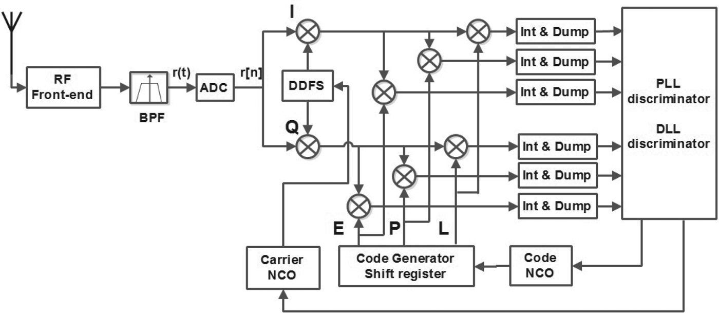
Figure 1 shows a GNSS receiver block diagram, where locally generated signals track the incoming signal by adjusting code and carrier Numerically Controlled Oscillators (NCOs). The performance of the receiver depends on the accuracy of this synchronisation.
Block diagram of a digital GNSS receiver.

The input to the digital part of the receiver is generally an Intermediate Frequency (IF) signal that is obtained by down-converting a Radio-Frequency (RF) signal. The front-end filter is approximated by an ideal pre-correlation filter (a rectangular Bandpass Filter (BPF)) centred at the IF frequency (f IF ) with two-sided bandwidth β r . One satellite's IF signal can be written as:
 $$r(t) = \sqrt {2C_{s}} \sum\limits_{k=-{\infty }}^{\infty }\, C_{\{ k\}_{N}} {\Pi}(t-kT_{c}(k)-\tau )d(t-\tau )cos(2\pi (f_{IF}+f_{D})t+\theta )+w{(t)}$$
where C s is the received signal power; Π is the rectangular function; C k = ±1 is the k th PRN code, {k} N is k modulus N, and N is the PRN code length (N = 1023 for GPS L1 C/A); T c (k) is the code chip duration that is varied by time due to the effect of the code Doppler or local oscillator drifts; d(t – τ) = ± 1 is the modulated navigation data bit; τ is the timing delay of received signal; f IF and f D denotes the IF frequency and the Doppler shift, respectively; θ is the random unknown carrier phase and w(t) is the Additive White Gaussian Noise (AWGN) with zero-mean and Power Spectral Density (PSD) N 0.
The IF signal is sampled by an Analogue-to-Digital Converter (ADC) which generates a sequence of samples r[nTs ], obtained by sampling r(t) at the sampling frequency f s = 1/T s . The notation r[n] = r[nTs ] indicates a discrete time sequence of the received signal r(t):
 $$\eqalign{ r[n] = &\sqrt {2C_{s}} \sum\limits_{k=-{\infty }}^{\infty } \, \sum\limits_{m=0}^{M-1} \, C_{\{k\}_{N}}\delta \left[n-m-\sum\limits_{j=-{\infty }}^{j=k-1} M_{j} -\lfloor\tau \rfloor_{T_{s}}\right]d[n-\lfloor\tau \rfloor_{T_{s}}] \cr & \times cos[2\pi (f_{IF}+f_{D})n+\hat{\theta}]+w[n]}$$
where δ is the Dirac delta function and
 $\lfloor\tau \rfloor_{T_{s}} = floor(\tau /T_{s})$
is the delay of the received signal after sampling. M
j
is the number of signal samples of the jth PRN code chip (MkTs
≤ Tc
(j)). M
j
is dependent on the f
s
/f
c
ratio and the residual code phase of that code chip, with f
c
being the local generated PRN code rate. θ̂ is the discrete time of the carrier phase. This phase discreteness is not considered as it does not affect the discussion topic. After Equation (2), θ̂ is replaced by θ here.
The PLL wipes off the carrier (Kaplan and Hegarty, Reference Kaplan and Hegarty2005) and the DLL synchronises the local and incoming PRN codes. The signal after the Direct Digital Frequency Synthesizer (DDFS) is down-converted to baseband and is ideally contained in only the in-phase (I) channel. The DLL tracks the time delay of the incoming PRN. The baseband signal is correlated with three local replica code-taps: Early (E), Prompt (P), and Late (L), through a multiplication and integration, usually over an integer PRN code period (T 0). Discriminator feedbacks adjust the Code NCO, which fluctuates the local replica code rate to synchronise with the incoming code (Parkinson, Reference Parkinson1996).
2.1. Residual code phase estimation
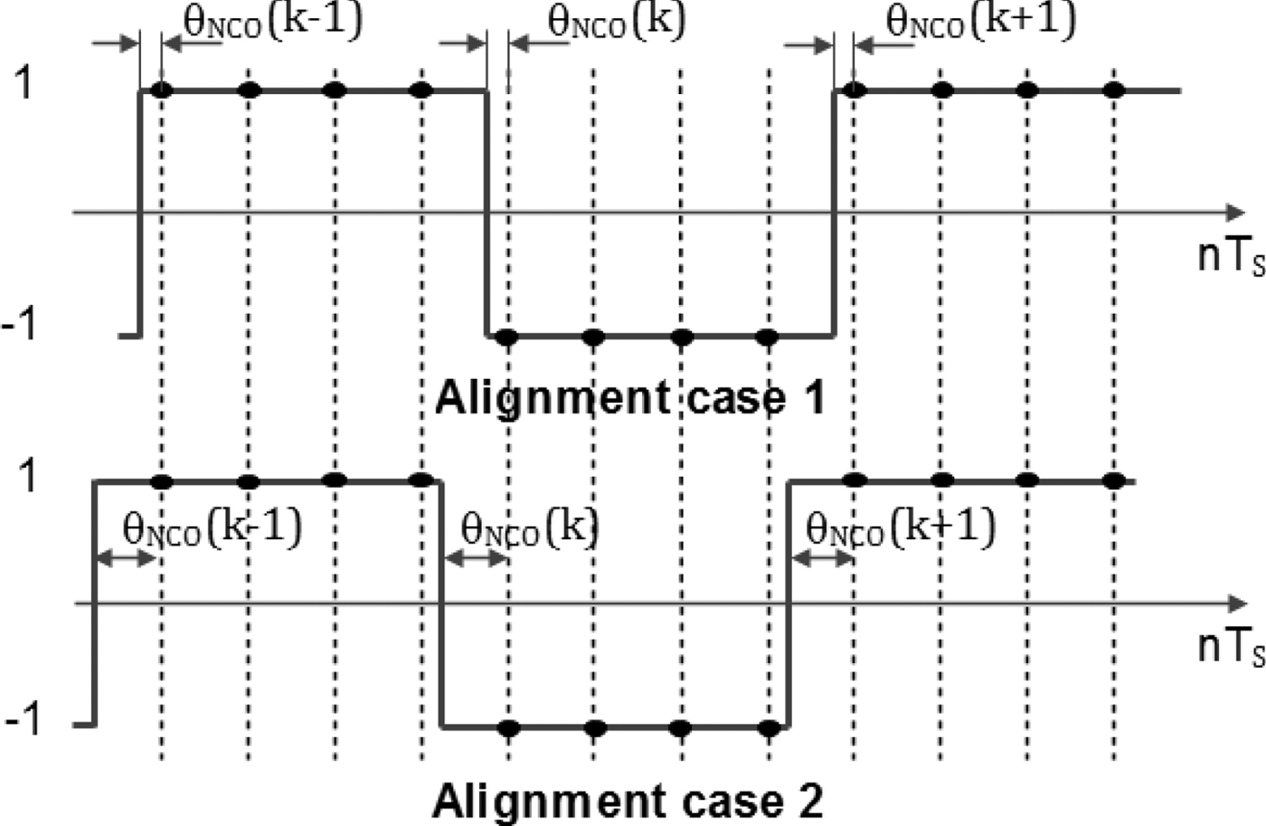
Estimating the pseudorange, used to calculate position, relies on the ability to locate the PRN code chip transition. The more precisely the transition is detected, the more accurate the user position. The residual code phase (θNCO ) is exploited to improve the accuracy.
Let η(m) denote the code NCO register contents at the mth clock tick, the NCO difference equation is:
 $$\eta (m) = \{\eta (m-1)+f_{c} /f_{s} \}_{1}$$
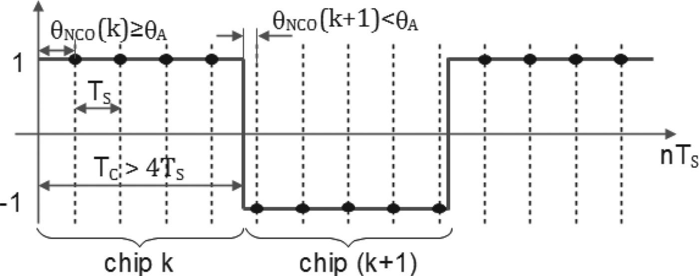
The register overflows once every n s = f c /f s samples on average, causing the PRN code generator to be clocked, incrementing the (k−1)th PRN code C k−1 to the kth PRN code C k . The NCO remaining content after this overflow is the residual code phase (θNCO (k)). It is equivalent to the delay between the start of the local kth chip and the first equivalent incoming signal sample or the so-called instantaneous chip phase, with 0 ≤ θNCO (k) < 1/ns .
The number of samples per code chip, n
s
, is generally a non-integer. Even if designed to be an integer, drifts in the local oscillator and Doppler shifts cause it to become a non-integer. The number of received signal samples correlated with the kth PRN code is either
 $\lfloor n_{s}\rfloor$
or
 $\lfloor n_{s}\rfloor +1$
, where the exact number is determined by a given θNCO
(k) as illustrated in Figure 2 and:
Residual code phases versus the number of samples per code chip with 4f c <f s <5f c .

 $$M_{k} = \left\{ \matrix{ \lfloor n_{s} \rfloor + 1 & (0 \le \theta_{NCO}(k) < \theta_{A}) \cr \lfloor n_{s} \rfloor \hfill & \quad (0 \le \theta_{NCO}(k) < 1/n_{s})} \right.$$
where
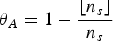 $\theta_{A}=1-{\lfloor n_{s} \rfloor \over n_{s}}$
and
 $\lfloor . \rfloor$
is the floor function. The residual code phase θNCO
(k) of each PRN code chip can be calculated as:
 $$\theta_{NCO} (k) = \left\{ \matrix{ {\theta_{NCO} ({k-1})+{\lfloor n_{s} \rfloor +1 \over n_{s}}-1} & {({0\le \theta_{NCO} ({k-1})< \theta_{A}})} \cr {\theta_{NCO} ({k-1}) + {\lfloor n_{s} \rfloor \over n_{s}}-1} \hfill & \quad {({\theta_{A} \le \theta_{NCO} ({k-1})< 1/n_{s}})}} \right.$$
where k is in the range [0, T 0 N − 1].
2.2. Correlation output calculation
Assume that the PLL is locked and the IF signal is ideally down-converted to baseband. If the incoming baseband signal is correlated with the local replica code for T seconds, or T0 code periods, and the navigation data bits
 $\bf{d[n-\lfloor\bf{\tau}\rfloor_{T_{s}}]}$
do not change, then the P tap correlation output is given by:
 $$\eqalign{ R(\tau) &= {C_s \over N_L}\sum^{N_L-1}_{n=0} \sum^{T_0N-1}_{k=0}\sum^{M_k-1}_{m=0} C_{\{k\}_N} \delta \left[n-m-\sum^{j=k}_{j=0}M_j-\lfloor\tau\rfloor_{T_s}\right] \cr &\quad \times \sum^{T_0 N-1}_{k=0}\sum^{M_k-1}_{m=0} C_{\{k\}_N} \delta \left[n-m-\sum^{j=k}_{j=0}M_j + \lfloor\theta_{NCO}(k) T_c\rfloor_{T_s}\right] \cr &= {C_s \over N_L}\sum^{N_L-1}_{n=0} \sum^{T_0N-1}_{k=0}\sum^{M_k-1}_{m=0} C_{\{k\}_N} \delta \left[n-m-\sum^{j=k}_{j=0}M_j-\lfloor\tau + \theta_{NCO}(k) T_c\rfloor_{T_s}\right] \cr &\quad \times \sum^{T_0 N-1}_{k=0}\sum^{M_k-1}_{m=0} C_{\{k\}_N} \delta \left[n-m-\sum^{j=k}_{j=0}M_j\right] }$$
where T
c
is the nominal code chip duration and
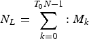 $N_{L} = \sum^{T_{0} N-1}_{k=0}{:}\ M_{k}$
is the total number of samples that are correlated and M
k
is the number of samples of the kth PRN code chip. The correlation output, as shown in Appendix A, is:
 $$R\lpar \tau \rpar = {C_{s} \over N_{L}} \sum\limits_{k=0}^{T_{0} N-1} \int\limits_{-\beta_{r} /2}^{\beta_{r} /2} T_{s} G_{s_{k}} (f)e^{i2\pi fT_{s} \lpar \lfloor\tau +\theta_{NCO} \lpar k \rpar T_{c}\rfloor_{T_{s}}\rpar }df$$
where
 $-T_{c} \le \lpar {\tau +\theta_{NCO} (k)T_{c}}\rpar \le T_{c}$
and
 $G_{s_{k}} (f)=T_{s} \lpar {{\sin \lpar {\pi fM_{k} T_{s}}\rpar \over \sin \lpar {\pi fT_{s}}\rpar }}\rpar ^{2}$
.
The PSD normalised to unit power of the sampling PRN code is:
 $${G_{s} (f)_{PSD} = {T_{s} \over N_{L}}\sum\limits_{k=0}^{T_{0} N-1} \left({{\sin \lpar {\pi fM_{k} T_{s}}\rpar \over \sin \lpar {\pi fT_{s}}\rpar }}\right)^{2} e^{i2\pi fT_{s} \lpar {\lfloor\theta_{NCO} \lpar k \rpar T_{c}\rfloor_{T_{s}}}\rpar }}$$
It is obvious that
 $\theta_{NCO} (k)T_{c} <T_{s}$
thus
 $\lfloor\theta_{NCO} (k)T_{c}\rfloor_{T_{s}} = 0$
and
 $$G_{s} (f)_{PSD} = {M_{k} \over N_{L}}\sum_{k=0}^{T_{0} N-1} {M_{k} T_{s} \sin^{2}\lpar {\pi fM_{k} T_{s}} \rpar \over M_{k}^{2} \sin^{2}\lpar {\pi fT_{s}} \rpar }$$
observe that
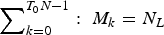 $\sum\nolimits_{k = 0}^{T_0N - 1} : \;M_k = N_L$
,
 ${\lim}_{f_{s} \to \infty } M_{k} T_{s}= T_{c}$
, and
 ${\lim}_{f_{s} \to \infty } \sin\lpar {\pi fT_{s}}\rpar =\pi fT_{s}$
so:
 $$\eqalign{ {\lim\limits_{f_{s} \to \infty} G_{s} (f)_{PSD}} & ={1 \over N_{L}}\sum\limits_{k=0}^{T_{0} N-1} M_{k} \lim\limits_{f_{s} \to \infty } \left({{M_{k} T_{s} \sin^{2}\lpar {\pi fM_{k} T_{s}} \rpar \over M_{k}^{2} \sin^{2}\lpar {\pi fT_{s}}\rpar }}\right) \cr &=T_{c} sin\,c^{2}\lpar {\pi fT_{c}}\rpar }$$
this is the well-known PSD proposed in (Parkinson, Reference Parkinson1996). This widely applied PSD equation is only correct when the sampling frequency is much higher than the PRN code rate.
3. EFFECT OF SAMPLING FREQUENCY ON CORRELATION SHAPE AND DLL DISCRIMINATOR FUNCTION
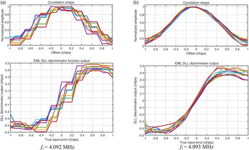
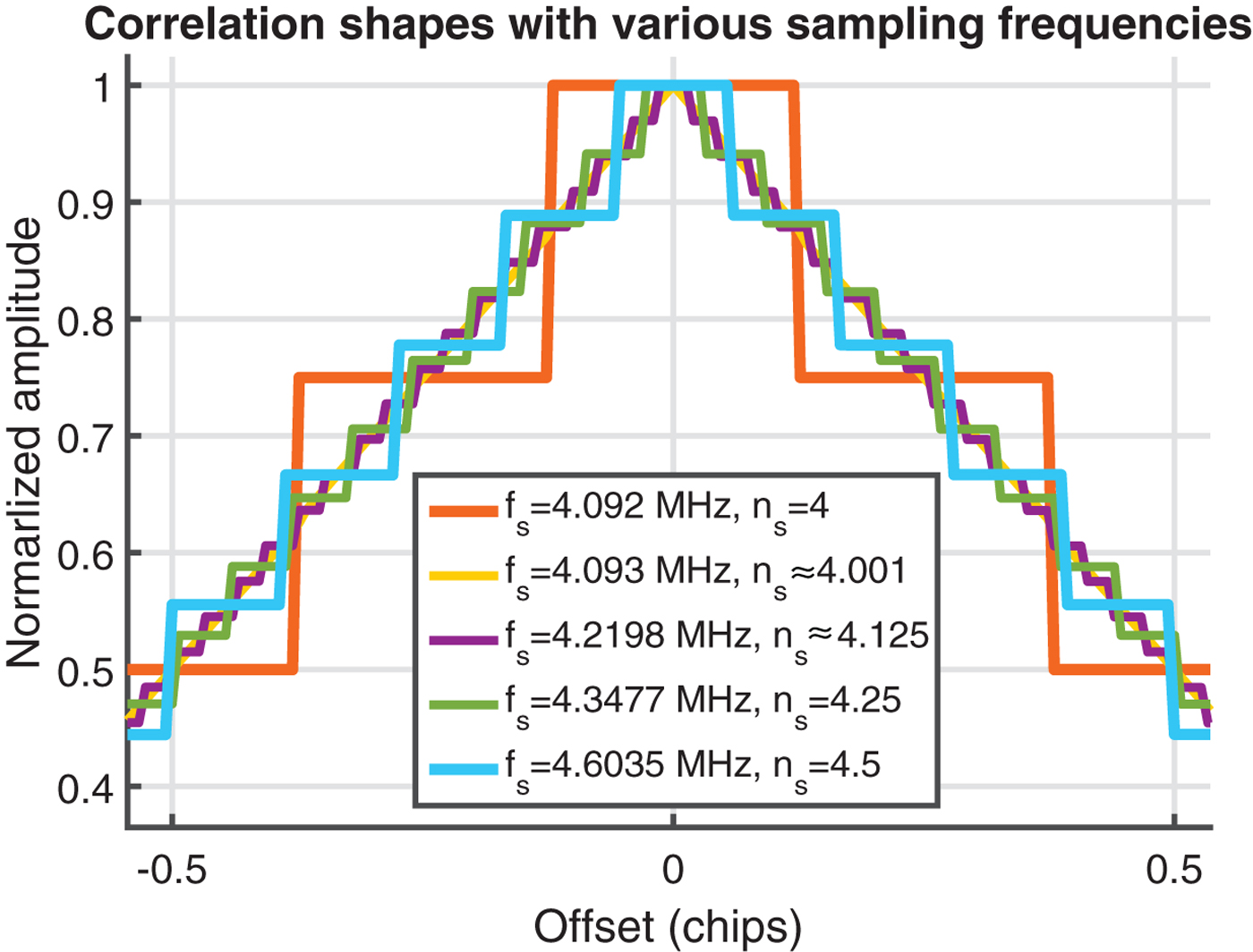
Figure 3 shows correlator shapes and EML discriminator outputs for 1 ms integrations of the incoming GPS L1 C/A signal with the P tap. Signals were received by a Nuand bladeRF front-end (Nuand-LLC, 2016) with two sampling frequencies fs = 4·092 and 4·093 MHz. Different colour results are illustrated for random instances of 1ms integrations. Step-like distortion of both functions can be easily observed for a commensurate sampling frequency (fs = 4·092 MHz). Oscillator drift and Doppler shifts can cause the sampling ratio to become non-integer, but not sufficiently to reduce this distortion. Distortions are absent for fs = 4·093 MHz, a 1 kHz difference, suggesting non-commensurate sampling frequencies do not suffer the distortions. However, this is not generally correct. Figure 4 shows correlator shapes obtained from Equation (7) at several sampling rates and random values of θNCO (0). The distortion still appears when the ratio f s /f c is non-commensurate.
Normalised correlator and EML discriminator functions for different sampling frequencies. Results are obtained by correlating the incoming signal with various local generated replica signals that have the time delay from–T c to T c with step = 10−2 T c .

Correlation shapes for 1 ms integration with various sampling frequencies.

3.1. Effect of the sampling frequency and the integration period selection
If Doppler shifts are zero and the sampling frequency is four-times the nominal PRN code rate, each analogue code chip always has four samples. Figure 5 shows that the same sample sequence can represent two different incoming code phases. The same correlation value is expected, despite real analogue signal alignments being different. This leads to the “staircase” correlation shapes.
Ambiguous synchronisation between a local PRN code and two different incoming analogue signals of the same PRN sequence, but with slightly differing code phase offset.

Higher residual code phase density with uniform distribution in the range [0, 1/n s ), gives a less distorted correlation shape, as shown in Figure 4. When fs = 4·093, the residual code phases have 1023 different values across [0, 1/n s ), with just one, two or four values for fs = 4·092 MHz (f s /f c = 4), fs = 4·6035 MHz (fs /fc = 4·5), or fs = 4·3477 MHz (fs /fc = 4·25), respectively.
An ideal sampling frequency, therefore, must be based on the distribution of distinct residual code phases. If fs
= M
0
fc
+ δ
fs
where
 $0 < \delta_{f_{s}} \ll f_{c}$
, M
o
is an integer, integration period is T ms (T
0 code periods), and θNCO
(0) = 0, from Equation (5) the number of different code phases, N
CP
, can be estimated as:
 $${N_{CP}} ={1-{\lfloor n_{s}\rfloor \over n_{s}} \over {\lfloor n_{s}\rfloor +1 \over n_{s}}-1} + {{1 \over n_{s}}-1-{\lfloor n_{s}\rfloor \over n_{s}} \over 1-{\lfloor n_{s}\rfloor \over n_{s}}} ={\delta_{f_{s}} \over f_{c} -\delta_{f_{s}}}+{f_{c} - \delta_{f_{s}} \over \delta_{f_{s}}}$$
because
 $0< \delta_{f_{s}} \ll f_{c}$
, Equation (11) can be approximated as:
 $N_{CP} \approx {f_{c} \over \delta_{f_{s}}}$
.
The number of correlatedcode chips (T
0
N) is also the maximum possible number of distinct residual code phases. If
 $\delta_{f_{s}} = {f_{c} \over T_{0} N}$
, the effect of correlation distortion is minimised. For instance, if the received signal is GPS L1 C/A and T = 1 ms, so δfs
= ± 1 kHz and the sampling frequency at fs
= 4·093 MHz produces the smoothest result as shown in Figure 4.
This result can also be used to estimate the minimum integration period required, e.g. if fs
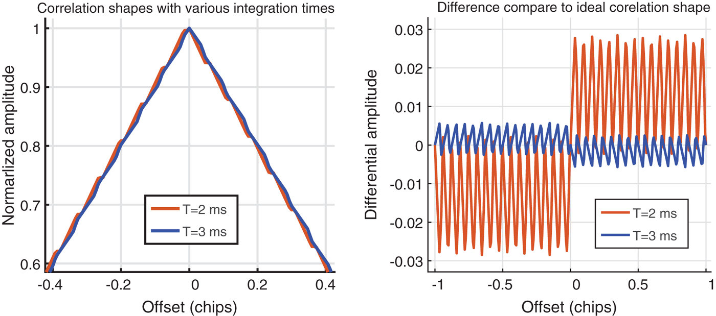
= 16·3676 MHz (NordNav Rxx2 receiver), the minimum required correlation time is T ≥ 2·5 ms. If T = 2 ms, the distortion is much higher - as presented in Figure 6. However, these estimates assume that
 $0 < \delta_{f_{s}} \ll f_{c}$
. When
 $\delta_{f_{s}}$
is greater, because of the random distribution, the number of distinct residual code phases cannot be directly estimated by the sampling frequency. The one-sigma coherent EML DLL error is analysed to further examine the effect of the sampling frequency in Section 4.
Correlation shapes and their errors with respect to the ideal correlation at a sampling frequency f s = 16·3676 MHz using various coherent integration periods.

3.2. Effect on the presence of Doppler and Local Oscillator (LO) clock drift
The effect of Doppler shifts and LO drifts on the incoming signal leads to offsets of the PRN code rate. Consequently, the number of samples per code chip is not an integer, even if the sampling frequency is commensurate. The LO reference frequency source for a GNSS receiver is often a Temperature Compensated Crystal Oscillator (TCXO), which typically has a one second Allan deviation of 10−7 and frequency stability of less than one part per million (ppm). If sampling frequency is fs = 4·092 MHz, the code frequency drift is less than 4 Hz. This LO drift is very small when the Doppler shift may be inline or reverse to the LO drift. The LO drift thus can be considered as an addition to the Doppler shift. The Doppler shift is, therefore, only mentioned in the following analyses, but it actually stands for the combination of Doppler shift and LO drift.
If the Doppler frequency, f
D
, is in the range [−10, 10] kHz, the corresponding code frequency varies between
 $[-6{\cdot}5, 6{\cdot}5]$
Hz. The code Doppler frequency, δfc
, can be estimated by
 $\delta_{f_{c}} ={f_{D} f_{c} \over f_{RF}}$
, where f
RF
is the carrier frequency. The code Doppler shift leads to variation of residual code phases, thus the correlator distortion will change as sampling rates drift into and away from commensurate values. The minimum Doppler frequency and coherent integration period, which flattens the correlation shape, can be evaluated by the number of distinct residual code phases. If the sampling frequency is commensurate, f
s
= M
0
f
c
, the real code rate is
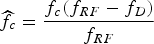 $\widehat{f_{c}} = {f_{c} \lpar {f_{RF} - f_{D}} \rpar \over f_{RF}}$
, with f
D
> 0. The number of distinct code phases is:
 $$N_{CP} = {{f_{s} \over {\widehat{f_{c}}^{\vphantom{0}}}} - {f_{s} \over f_{c}} \over {f_{s} \over f_{c}}+1-{f_{s} \over {\widehat{f_{c}}^{\vphantom{0}}}}}+{{f_{s} \over f_{c}}+1-{f_{s} \over {\widehat{f_{c}}^{\vphantom{0}}}} \over {f_{s} \over {\widehat{f_{c}}^{\vphantom{0}}}}-{f_{s} \over f_{c}}}$$
because
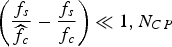 $\left({{f_{s} \over {\widehat{f_{c}}}^{}} - {f_{s} \over f_{c}}}\right)\ll 1, N_{CP}$
can be approximated as:
 $${N_{CP}} \approx {f_{c} \widehat{{f_{c}}} \over f_{s} \lpar {f_{c} -{\widehat{f_{c}}}}\rpar } ={f_{c} \lpar {f_{RF} -f_{D}} \rpar \over f_{s} f_{D}}$$
The maximum number of distinct residual code phases is the number of correlated code chips. If N CP = T o N, the correlation shape is the smoothest. The relation between integration period T (equal to T 0 PRN code periods) and Doppler frequency (f D ), therefore, must fulfil:
 $$f_{D} = {f_{c} f_{RF} \over f_{s} T_{0} N+f_{c}}$$
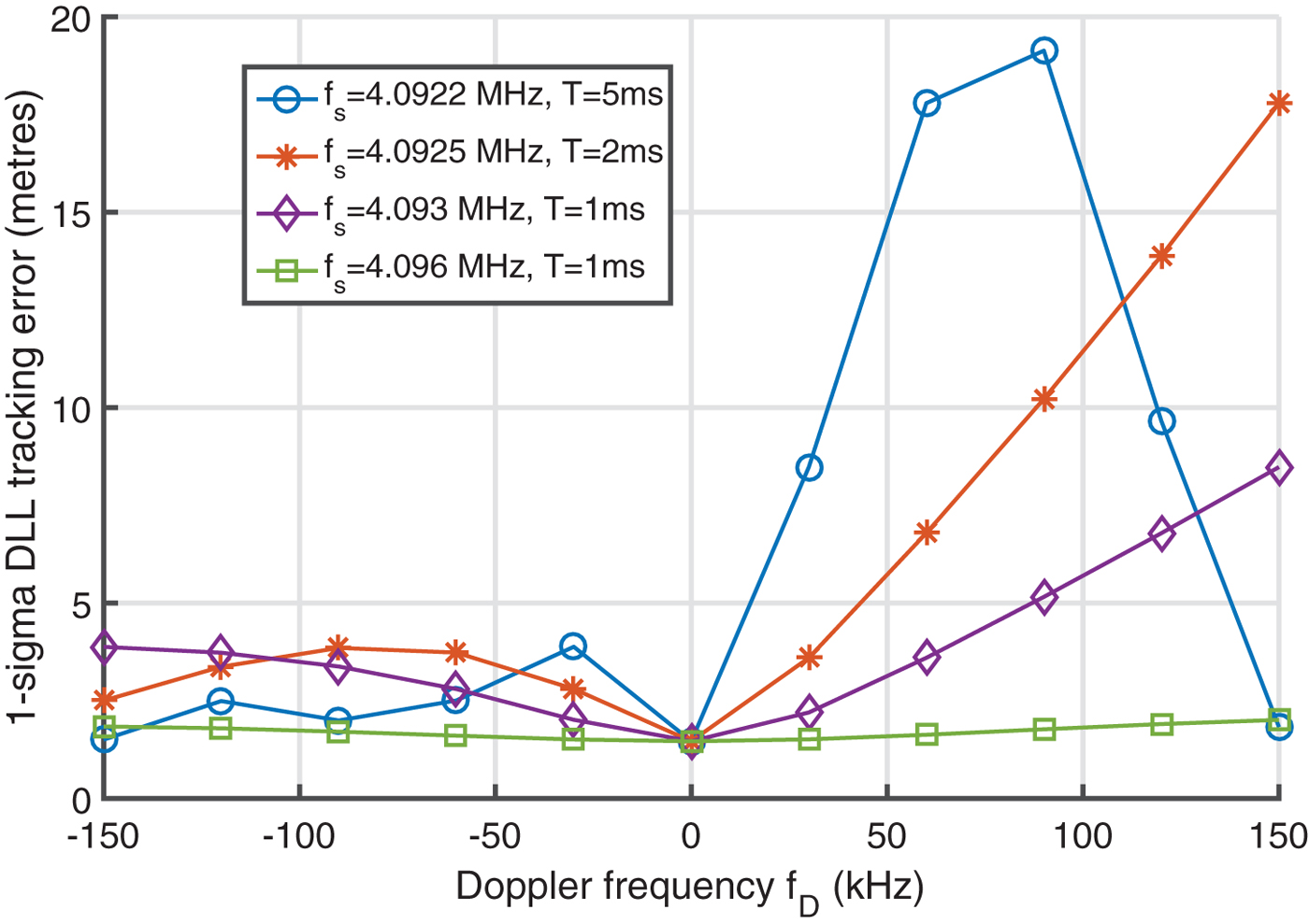
For example, if the received signal is GPS L1 C/A, fRF = 1575·42 MHz, fs = 4·092 MHz (n s = 4), and integration period T = 1 and 10 ms, the Doppler frequency must be fD ≥ 384·91 kHz and 38·5 kHz, respectively. This is out of most terrestrial receivers’ Doppler range, [−10, 10] kHz. If the Doppler is f D = 2 kHz, the integration period must be T ≥ 192·5 ms. However, the coherent integration period should be smaller than 20 ms or 10 ms, with or without data bit synchronisation, respectively, or may be shorter due to secondary code transitions (Tran et al., Reference Tran, Shivaramaiah and Dempster2015; Shivaramaiah et al., Reference Shivaramaiah, Dempster and Rizos2008). High Doppler frequencies, high LO drifts, and long integration periods such as tracking a data-less (Pilot) channel can help to reduce the correlation and discriminator distortions, but a typical receiver usually has a stable LO and a short integration period (T ≤ 20 ms) for tracking, thus the effect of sampling frequency should be considered for every Doppler frequency. On the other hand, if the difference of the sampling frequency to an integer multiple of the nominal code rate, δ fs , is too small, a high Doppler frequency can lead to the distortion. For example, if fs = 4·0922 MHz (δ fs = 0·2 kHz), Doppler fD ≈ 77 kHz causes the number of samples per code chip to become n s = 4 and the distortion thus occurs. This will be analysed in the next section.
4. COHERENT EARLY MINUS LATE DLL ERROR ANALYSIS
The selection guideline for the sampling frequency and integration period is only valid for
 $0 < {\bf \delta}_{f_s} \ll f_c$
, as mentioned in Section 3.1. Therefore, the coherent EML DLL tracking error will be analysed to further examine effects of the sampling frequency, front-end bandwidth, coherent integration periods, and Doppler shifts in this section.
4.1. Theoretical code tracking loop error estimate
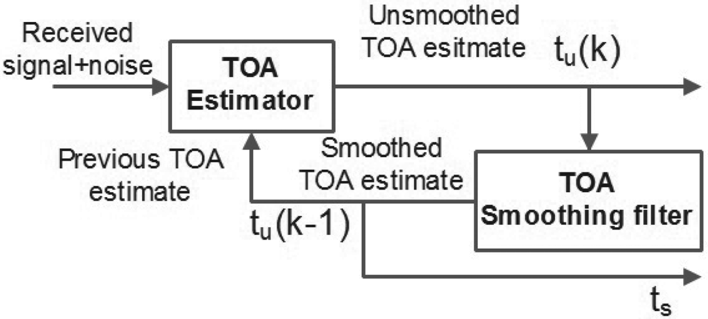
In this paper, the code tracking loop uses the model that was proposed by Betz and Kolodziejski (Reference Betz and Kolodziejski2000; Reference Betz and Kolodziejski2009a; Reference Betz and Kolodziejski2009b) which is re-illustrated in Figure 7. The Time Of Arrival (TOA) estimator uses an integration period of T seconds to produce an unsmoothed TOA estimate from the received signal plus noise. This estimate is used to update the previous TOA estimate. Using a code-tracking loop that acts like a TOA smoothing filter, producing smoothed TOA estimates.
Representation of code tracking loop (Betz and Kolodziejski, Reference Betz and Kolodziejski2009a).

According to Betz and Kolodziejski (Reference Betz and Kolodziejski2009a), the variance of the unsmoothed TOA estimate from the discriminator is
 $\sigma_{u}^{2}$
, and the variance of the smoothed TOA estimate at the output of the code tracking loop, denoted as
 $\sigma_{s}^{2}$
, is:
 $$\sigma_{s}^{2} \cong \sigma_{u}^{2} 2B_{L} T$$
where B L is the noise bandwidth of the DLL tracking loop, T is the integration period, and 0 < BLT ≤ 0·5. It should be noted that a factor of (1–0·5BLT) appears in Equation (2) of Betz and Kolodziejski (Reference Betz and Kolodziejski2009a). In fact, this term originates from a flaw from that work as detailed by Zhang and Zhan (Reference Zhang and Zhan2012), thus it has been omitted here.
This estimation does not accurately consider the effect of the sampling frequency. Therefore, it is re-considered here with the errors broken into two components, namely the part that is influenced by the sampling frequency (
 $\sigma_{1}^{2}$
and
 $\sigma_{2}^{2}$
) and the part that is effected by the code lock loop noise filter (
 $\sigma_{u1N}^{2}$
and
 $\sigma_{u2N}^{2}$
). A detailed analysis is shown in Appendix B.
The variance of the unsmoothed TOA estimate,
 $\sigma_{u}^{2}$
, is bounded between
 $\sigma_{u1}^{2}$
and
 $\sigma_{u2}^{2}$
, whose values are:
 $$\sigma_{u1}^{2} = \sigma_{1}^{2} + \sigma_{u1N}^{2}$$
 $$\sigma_{u2}^{2} = \sigma_{2}^{2} + \sigma_{u2N}^{2}$$
where:
 $$\sigma_{1}^{2} = {\left(\sum\nolimits_{k=0}^{T_{0} N-1} {1 \over N_{L}} \int\nolimits_{-\beta_{r} /2}^{\beta_{r}/2}G_{s_{k}}(f)\sin \lpar {\pi f\!\!{\Delta}}\rpar \sin \lpar {\pi f\lpar {2\theta_{NCO} \lpar k \rpar T_{c} -T_{s}} \rpar }\rpar \cos\lpar {\pi fT_{s}}\rpar df\right)^{2} \over \left({\sum\nolimits_{k=0}^{T_{0} N-1} {2\pi \over N_{L}}\int\nolimits_{-\beta_{r}/2}^{\beta_{r}/2}fG_{s_{k}}\lpar f \rpar \sin \lpar {\pi f\!\!\Delta}\rpar \cos \lpar {2\pi f\theta_{NCO} \lpar k \rpar T_{c}} \rpar df}\right)^{2}}$$
 $$\sigma_{2}^{2} ={\left({\sum\nolimits_{k=0}^{T_{0} N-1} {1 \over N_{L}}\int\nolimits_{-\beta_{r} /2}^{\beta_{r} /2} {{G_{s_{k}} \lpar f \rpar \sin \lpar {\pi f\!\!\Delta} \rpar \sin \lpar {\pi f\lpar {2\theta_{NCO} (k)T_{c} -T_{s}} \rpar } \rpar \cos \lpar {\pi fT_{s}} \rpar df}}}\right)^{2} \over \left({\sum\nolimits_{k=0}^{T_{0} N-1} {2\pi \over N_{L}}\int\nolimits_{-\beta_{r} /2}^{\beta_{r} /2} {fG_{s_{k}} \lpar f \rpar \sin \lpar {\pi f\!\!\Delta } \rpar \cos \lpar {2\pi f( {\theta_{NCO} \lpar k \rpar T_{c} -T_{s}} )} \rpar df}}\right)^{2}}$$
 $$\eqalign{ {\sigma_{u1N}^{2}} &= {{N_{0} \over 2C_{s} N_{L}}\sum\nolimits_{k=0}^{T_{0} N-1} -\int\nolimits_{-\beta_{r} /2}^{\beta_{r} /2} {G_{s_{k}} \lpar f \rpar \sin ^{2}\lpar {\pi f\!\!\Delta } \rpar df} \over \left({\sum\nolimits_{k=0}^{T_{0} N-1} {2\pi \over N_{L}}\int\nolimits_{-\beta_{r} /2}^{\beta_{r} /2} {fG_{s_{k}} \lpar f \rpar \sin \lpar {\pi f\!\!\Delta } \rpar \cos \lpar {2\pi f\theta_{NCO} \lpar k \rpar T_{c}} \rpar df}}\right)^{2}}}$$
 $$\eqalign{ {\sigma_{u2N}^{2}} &= {{N_{0} \over 2C_{s} N_{L}}\sum\nolimits_{k=0}^{T_{0} N-1}- \int\nolimits_{-\beta_{r} /2}^{\beta_{r} /2} {G_{s_{k}} \lpar f \rpar \sin ^{2}\lpar {\pi f\!\!\Delta } \rpar df} \over \left( {\sum\nolimits_{k=0}^{T_{0} N-1} {2\pi \over N_{L}}\int\nolimits_{-\beta_{r} /2}^{\beta_{r} /2} {fG_{s_{k}} \lpar f \rpar \sin \lpar {\pi f\!\!\Delta } \rpar \cos \lpar {2\pi f\lpar {\theta_{NCO} \lpar k \rpar T_{c} -T_{s}} \rpar } \rpar df}}\right)^{2}}}$$
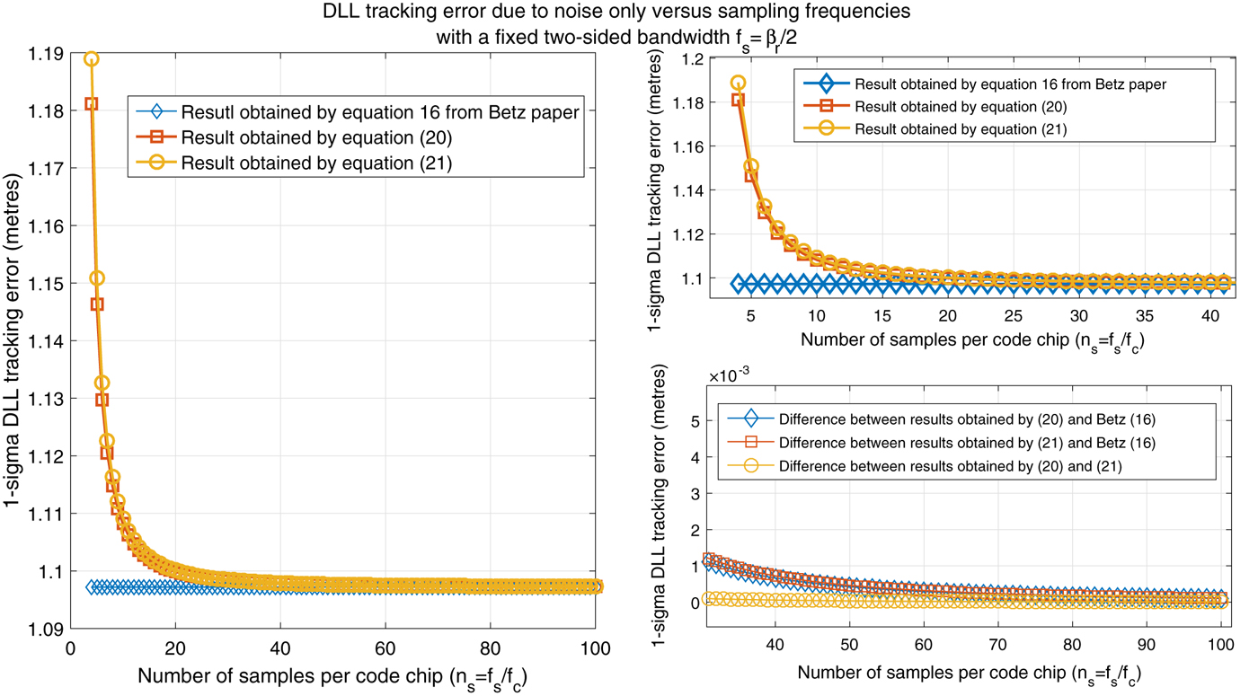
It can be mathematically observed that when the sampling frequency is infinite,
 $\theta_{NCO} (k)\cong 0$
for all k and T
s
≅ 0 the cosine value appearing in the denominator of Equations (20) and (21) is approximately one. This estimation becomes the same as the results presented in Equation (16) of Betz and Kolodziejski (Reference Betz and Kolodziejski2009a). The analysis comparison results presented in Figure 8 further strengthens this state.
DLL jitter versus different sampling frequencies (step = f c ) for a GPS L1 C/A with C/N 0 = 40 dB-Hz, B L = 0·5 Hz, T = 1 ms, and fixed BW β r = 2f c .

Both
 $\sigma_{1}^{2}$
and
 $\sigma_{2}^{2}$
, as shown in Equations (18) and (19), have approximately constant bias during tracking. The DLL noise filter has no effect on these values. Only the error contributed by noise
 $\sigma_{u1N}^{2}$
and
 $\sigma_{u2N}^{2}$
are filtered by the tracking loop filter. Consequently, the one-sigma code tracking jitter (in metres) also varies between σ
s1 and σ
s2, where:
 $${\sigma_{s1}} = C\sqrt{\sigma_{1}^{2} +\sigma_{u1N}^{2} 2B_{L} T}$$
 $${\sigma_{s2}} = C\sqrt{\sigma_{2}^{2} +\sigma_{u2N}^{2} 2B_{L} T}$$
where C is the speed of light.
Note that
 $\sigma_{1}^{2}$
and
 $\sigma_{2}^{2}$
are constrained by the residual code phase θNCO
(k), while the initial residual code phase θNCO
(0) can have any random value in the range [0, 1/n
s
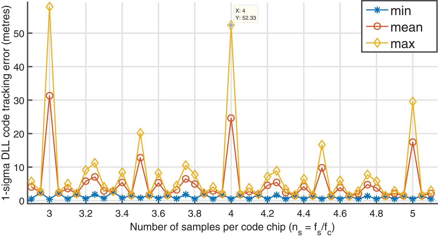
), so the code tracking loop error is altered. Figure 9 illustrates the maximum, minimum and mean values of σ
s1 versus sampling frequencies while the residual code phase varies. Take n
s
= 4 as an example, where the residual code phase is a constant for all code chips. The DLL jitter varies between the minimum value (≈ 0·47 m), when θNCO
(0) = 0, and the maximum value (≈ 52·3 m) when θNCO
(0) ≈ 1/ns
. Since θNCO
(0) is uniformly distributed in the range [0, 1/n
s
), the code tracking loop jitter can be approximated by the mean value of σ
s1 or σ
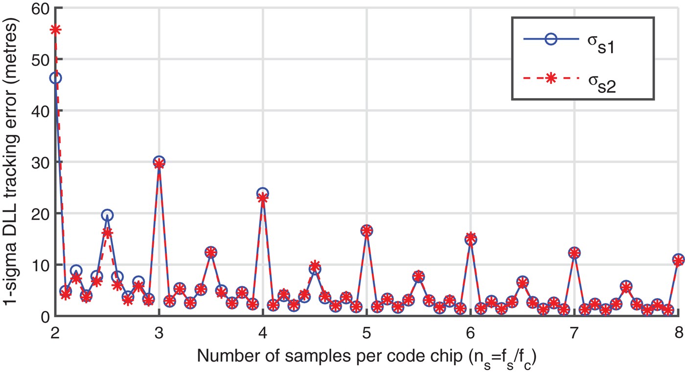
s2. Figure 10 presents the mean value of σ
s1 or σ
s2 versus different sampling frequencies. The two values are approximately equal for most sampling frequencies, so for easy comparison only the mean value of σ
s1 will be used for the remainder of the paper.
Upper bound and lower bound of the DLL jitter versus different sampling frequencies (step = 5*10−2 f c ) for a GPS L1 C/A with C/N 0 = 45 dB-Hz, B L = 0·5 Hz, T = 1 ms, and β r = f s .

Mean values of two error bounds σ s1 and σ s2 versus different sampling frequencies (step = 10−1 f c ) for a GPS L1 C/A with C/N 0 = 45 dB-Hz, B L = 0·5 Hz, T = 1 ms, and β r = f s .

4.2. Evaluation of theoretical results by simulated and numerical models
In this section, the simulated and numerical models used to estimate the DLL tracking loop errors are presented. The theoretical result is calculated for GPS L1 C/A using Equation (22) with the following assumptions: the received signal has no AWGN, the front-end has an ideal filter with the two-sided bandwidth β r = f s and the coherent integration period is T = 1 ms.
In the simulated model, the received pseudo-analogue signal was simulated by a sampled PRN code that was generated with frequency f
so
= 100 f
s
. After that, it was passed through a decimator that simulates a front-end ADC with two-sided bandwidth βr
≈ fs
and a sampling frequency f
s
. This digital signal was then correlated with two locally generated E and L signals that are one code chip delayed. The desired timing offset between received and local generated signals, τ0, was varied in the range [−T
c
, T
c
] with step δτ = 10-6
Tc
. The discrimination function
 ${{\rm E}\,{-}\,{\rm L} \over 2\lpar {\rm E}\,{+}\,{\rm L}\rpar }$
, is used toestimate the timing offset between the incoming signal and the local replica, τ
u
. Finally, the DLL jitter (in metres) is estimated by the variance of the difference between τ0 and τ
u
as follows:
 $$\sigma_{s} = CT_{c} \sqrt {var\lpar {\tau_{u} -\tau_{0} } \rpar }$$
The numerical model DLL jitter was calculated by using the same estimation model. The E and L correlator outputs were computed by Equation (7) with τ = −0·5 Tc
and 0·5 T
c
, respectively. The DLL jitter
 $\hat{\sigma}_{s}$
is the mean of σ
s
while the initial residual code phase θNCO
(0) varies in the range [0, 1/n
s
).
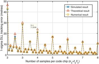
Figure 11 illustrates the DLL tracking errors of these three models. It is clear that the three different models provide approximately the same results, for various sampling frequencies. This reinforces the correctness of the proposed theoretical model.
DLL tracking error comparison among the simulated, numerical and theoretical models (step = 10−1 f c ) for a GPS L1 C/A with T = 1 ms, and β r = f s .

4.3. Effect of Doppler and coherent integration period
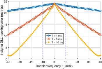
Figure 12 illustrates the DLL tracking error versus Doppler frequency, f D , for different coherent integration periods, T of a GPS L1 C/A signal with the received signal C/N 0 = 40 dB-Hz; the sampling frequency fs = 4·092 MHz (n s = 4), and the ideal brick-wall ADC filter with two-sided bandwidth β r = f s . The presence of Doppler helps to minimise the DLL error if the sampling frequency is commensurate; however, Doppler shifts must be very high, for example fD ≥ 38·5 kHz when T = 10 ms, this is out of typical Doppler range [−10, 10] kHz.
DLL tracking error versus Doppler frequencies f D for different integration periods T when the sampling frequency is an integer multiple of the nominal code rate (n s = 4), in which the blue dotted lines indicate the typical Doppler range.

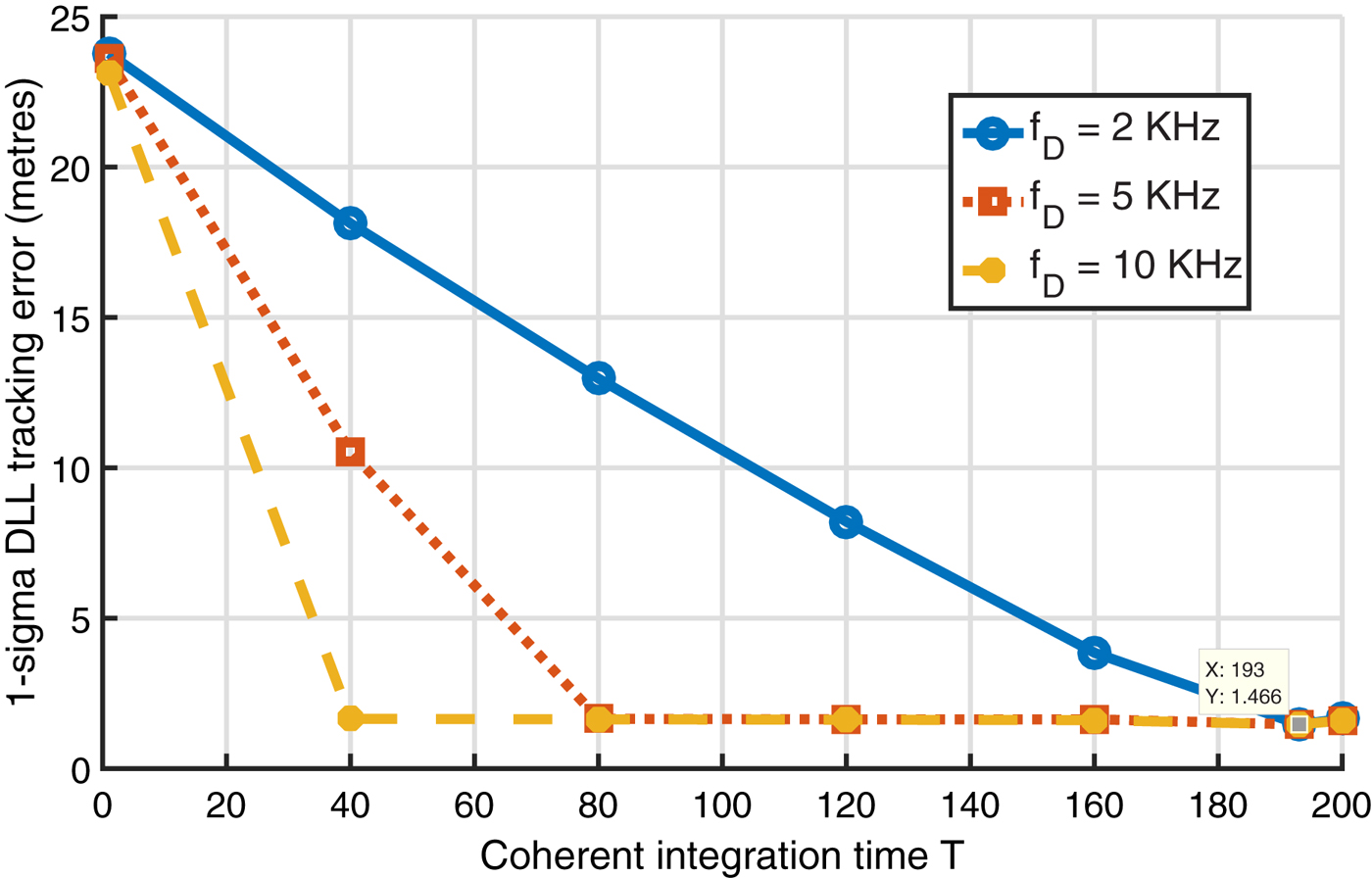
If the navigation data bit has been wiped-off, the coherent integration period is not limited. Figure 13 describes the DLL tracking error versus the integration period, T, for different Doppler frequencies. Observe that, if the sampling frequency fs = 4·092 (ns = 4) and the Doppler frequency f D = 2 kHz, the DLL error is a minimum when integration period T > 193 milliseconds. This result is equivalent to the predicted theoretical result shown in Section 3.2. Similarly, the DLL jitter is also lowest when T ≥ 40 and 80 milliseconds while f D = 5 and 10 kHz, respectively.
DLL tracking error versus integration periods T. GPS L1 C/A is used with f s = 4·092 MHz (n s = 4), C/N 0 = 40 dB-Hz, B L = 0·5 Hz, T = 1 ms, and β r = f s .

If the sampling ratio f s /f c is non-integer, but the frequency difference δ fs from an integer multiple of the code rate is small, the code rate drift caused by the high Doppler frequency leads to accuracy degradation, as shown in Figure 14. This high Doppler environment does not occur on a terrestrial GNSS receiver, but may exist on a space-borne receiver, and it needs to be considered while selecting front-end sampling frequencies and integration periods.
DLL tracking error versus Doppler frequencies f D for different integration periods T when the sampling frequency is a non-integer multiple of the nominal code rate.

To sum up, a very high Doppler frequency or a long coherent integration period can reduce the correlator and discriminator distortions (that is, minimise the DLL jitter) if the number of samples per code chip is an integer. However, if the sampling frequency is non-commensurate, a very high Doppler can lead to accuracy degradation. Therefore, the effect of the sampling frequency and integration periods on the receiver performance must be carefully considered for all Doppler frequencies.
Effect of the front-end filter bandwidth and the received C/N 0
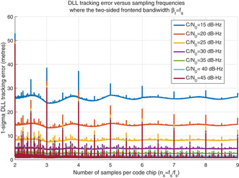
Figure 15 presents the DLL error versus different sampling frequencies for various C/N 0 when the two-sided bandwidth is fixed βr = 2fc (for example βr = 2·046 MHz for GPS L1 C/A signal). Observe that the one-sigma DLL tracking error is higher when the received signal is weak (C/N 0 = 10, 15, 20 dB-Hz). It is much smaller when the received C/N 0 is in the commonly received C/N 0 range (from 25 dB-Hz to 45 dB-Hz), which is equivalent to results presented in Kaplan and Hegarty (Reference Kaplan and Hegarty2005). The other observable trend is that the DLL error decreases when the sampling frequency increases. The more samples that are used to represent the incoming and local generated signals, the greater the accuracy at which the code chip transition can be detected. However, the DLL error is still significant at some peak points due to the effect of sampling frequencies. It is considerable for every received C/N 0, but it is much more visible when the received signal is strong (C/N 0 > 30 dB-Hz). This error cannot be observed if the DLL tracking error estimation proposed by Betz and Kolodziejski (Reference Betz and Kolodziejski2009a; Reference Betz and Kolodziejski2009b) is applied. Moreover, this DLL error is not only significant when the sampling rate is commensurate, but it is also considerable, when the ratio f s /f c is at some non-commensurate values. Therefore, the effect of the sampling frequency should be taken into account when choosing the front-end ADC sampling rate.
DLL tracking error versus different sampling frequencies (step = 10−3 f c ) with a fixed front-end bandwidth β r = 2f c for a GPS L1 C/A signal with B L = 0·5 Hz and T = 1 ms.

The DLL tracking errors versus sampling frequencies with different two-sided front-end bandwidths βr = 2fc and β r = f s are illustrated in Figures 15 and 16, respectively. Observe that the DLL error decreases when the sampling frequency increases if the front-end bandwidth is fixed, βr = 2fc (Figure 15). This is because the noise power is only governed by the front-end bandwidth, the coherent integration period, and it is not affected by the sampling frequency, as shown in Equation (20). The DLL error contributed by the noise power is thus the same when the sampling frequency increases. Consequently, the DLL error, excluding the peak impacted by the sampling frequency, is reduced when the sampling frequency is higher. However, this DLL tracking error is approximately constant if the front-end bandwidth is increased due to the sampling frequency, β r = f s (Figure 16). The wider the front-end bandwidth, the greater the received signal power, but the received signal also includes AWGN so noise power is also increased. Consequently, the DLL tracking noise error fluctuates slightly, but remains unchanged in general. Because the DLL error reduction, which occurs by increasing the sampling frequency and front-end bandwidth, is approximately offset by the error increase due to the growth of the noise power, the DLL error is much more visible when the received signal power is weak (C/N 0<30 dB-Hz).
DLL tracking error versus different sampling frequencies (step = 10−3 f c ) with front-end bandwidths β r = f s for a GPS L1 C/A signal with B L = 0·5 Hz and T = 1 ms.

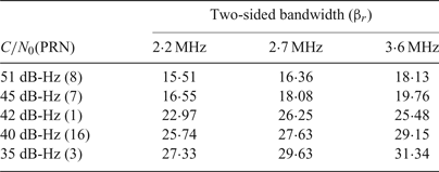
Experiments were set up to validate these conclusions. A Nuand bladeRF front-end was used to collect live GPS L1 C/A signal from a rooftop active antenna. A sampling frequency was chosen at fs = 4·092 MHz (n s = 4) and the signal was processed with various In-phase (I) and Quadrature (Q) front-end bandwidths of 1·5, 1·75 and 2·5 MHz, which is equivalent to the actual complex front-end bandwidth βr ≈ 2·2, 2·7, and 3·6 MHz, respectively. The DLL tracking error was calculated as the variance of 10,000 DLL discriminator outputs with a coherent integration period T = 1 ms and the noise bandwidth B L = 0·5 Hz. A uBlox 6T simultaneously processed the received signal to estimate the C/N 0 of each satellite. The experimental result, as presented in Table 1, validates the previous theoretical analysis that the narrower the front-end bandwidth, the smaller the DLL tracking error. Furthermore, the DLL tracking errors, as shown in Table 1 when the C/N 0 is 45, 42, 40 and 35 dB-Hz, are matched with the theoretical results presented in Figure 15 and Figure 16 where the number of samples per code chip n s = 4.
DLL tracking error (standard deviation in metres) versus different two-sided front-end bandwidths. A live GPS L1 C/A signal is recorded by the Nuand bladeRF front-end and processed with DLL tracking parameters BL = 0·5 Hz, T = 1 ms.

All in all, the effect of front-end bandwidth also needs to be considered in addition to the effect of the sampling frequency and the received C/N 0. Increasing the sampling frequency helps to reduce the DLL tracking error, and it is more effective for weak signals if and only if the front-end bandwidth is fixed and much smaller than the sampling frequency.
5. CONCLUSION
Sampling frequency has a strong influence on the synchronisation of the incoming and local generated signals and the code DLL tracking. The number of distinct residual code phases of each code chip and their distribution along the code phase range [0, 1/n s ) is the main cause of the correlation and discriminator distortions, that was practically observed by Thomas (Reference Thomas1988) for one specific sampling frequency. The DLL tracking error is not only considerable when the sampling frequency is commensurate, but also non-commensurate if the number of distinct residual code phases is low. The calculation of the number of distinct residual code phases in Section 3 and the theoretically proposed coherent EML DLL tracking error estimation in Section 4 further confirm this effect and can be used as a theoretical guideline for the sampling frequency and the coherent integration period selection.
The Doppler frequency can help to reduce the distortion caused by a bad sampling frequency choice; however, it is only valid if the Doppler frequency is very high, such as in a very high dynamic environment, or if the coherent integration is very long, such as when the navigation data bit transitions were predicted, or for a data-less (Pilot) channel. For a terrestrial receiver, the Doppler frequency has an insignificant effect on reducing the DLL errors because of the coherent integration that is limited by the secondary code or data bit transition.
The impact of the sampling frequency on correlation output, which is usually presented by the sampling filter bandwidth when the number of samples per code chip is assumed to be infinite, has been accurately calculated based on the number of samples per code chip in Section 2. The well-known DLL tracking error estimation proposed by Betz and Kolodziejski (Reference Betz and Kolodziejski2000; Reference Betz and Kolodziejski2009a; Reference Betz and Kolodziejski2009b) has been revised under the effect of the sampling frequency in Section 4. A more accurate estimation model has been proposed and proved mathematically (as shown in Appendix B). The previous estimation could not indicate the bias error constrained by the sampling frequency, whereas the proposed method cannot only cover the conventional DLL tracking error influenced by the noise power, but also illustrates the effect of the sampling frequency.
The front-end ADC filter bandwidth also has a strong effect on the DLL jitter. The DLL tracking error is decreased while the sampling frequency is increased and it is more efficient for weak signals (C/N 0<30 dB-Hz) if and only if the front-end bandwidth is fixed and much smaller than the sampling frequency.
APPENDIX A. CORRELATION OUTPUT CALCULATION
The local replica PRN can be illustrated as:
 $$C_{local} \lpar n \rpar =\mathop \sum\limits_{k=0}^{T_{0} N-1} \sum\limits_{m=0}^{M_{k} -1} C_{\{k\}_{N} } \delta \lsqb {n-m-N_{M_{k} } } \rsqb $$
where
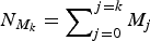 $N_{M_{k}} = \mathop \sum\nolimits_{j=0}^{j=k} M_{j}$
. Applying discrete time Fourier transform on the local replica PRN with
 $\romega = 2\pi fT_{s}$
:
 $$\eqalign{ C\lpar \omega \rpar &=\mathop \sum\limits_{n=-\infty }^{\infty } \sum\limits_{k=0}^{T_{0} N-1} \sum\limits_{m=0}^{M_{k} -1} C_{\{k\}_{N} } \delta \lsqb {n-m-N_{M_{k} } } \rsqb e^{-i\omega n} \cr &=\mathop \sum\limits_{k=0}^{T_{0} N-1} C_{\{k\}_{N} } e^{-i\omega N_{M_{k}}}\sum\limits_{m=0}^{M_{k} -1} e^{-i\omega m}\sum\limits_{n=-\infty }^{\infty } \delta \lsqb n \rsqb \cr &=\mathop \sum\limits_{k=0}^{T_{0} N-1} C_{\{k\}_{N} } e^{-i\omega kN_{M_{k}}}{sin\lpar {M_{k} \omega /2} \rpar \over sin\lpar {\omega /2} \rpar }e^{-i{\lpar {M_{k} +1} \rpar \omega \over 2}}}$$
so it can be illustrated in the frequency domain as:
 $${C(f)} =\sum\limits_{k=0}^{T_{0} N-1} C_{\{k\}_{N} } e^{-i2\pi fT_{s} N_{M_{k}}}{sin\lpar {M_{k} \pi fT_{s}} \rpar \over sin\lpar {\pi fT_{s}} \rpar }e^{-i\lpar {M_{k} +1} \rpar \pi fT_{s}}$$
and its reverse Fourier transform is:
 $$\sum\limits_{k=0}^{T_{0} N-1} \sum\limits_{m=0}^{M_{k} -1} C_{k} \delta \lsqb {n-m-N_{M_{k}}} \rsqb =T_{s} \int\limits_{-\beta_{r} /2}^{\beta_{r} /2} C\lpar f \rpar e^{i2\pi fT_{s} n}df$$
where β r is the receiver front-end bandwidth.
Substituting Equation (A4) into Equation (6), yields
 $$\eqalign{ R(\tau ) &= {{C_sT_s} \over {N_L}}\sum\limits_{n = 0}^{N_L - 1} {\sum\limits_{k = 0}^{T_0aN - 1} {\sum\limits_{m = 0}^{M_k - 1} {C_{{\{ k\} }_N}} } } \delta \lsqb {n - m - N_{M_k} - {\lfloor{\tau + \theta_{NCO}(k)T_c} \rfloor }_{T_s}} \rsqb \int\limits_{ - \beta _r/2}^{\beta _r/2} C (f)e^{i2\pi fT_sn}df \cr &={C_{s}T_{s} \over N_{L}}\int\limits_{-{\beta_{r} \over 2}}^{\beta_{r}/{2}} {\sum\limits_{n=0}^{N_{L}-1}} C(f)\sum\limits_{k=0}^{T_{0}N-1} \sum\limits_{m=0}^{M_{k}-1} C_{\{k\}_{N}}\delta [n-m-N_{M_{k}}-\lfloor\tau +\theta_{NCO}(k)T_{c} \rfloor_{T_{s}}]e^{i2\pi fT_{s}n}df \cr &\cong {C_{s}T_{s} \over N_{L}}\int\limits_{-\beta_{r}/2}^{\beta_{r}/2} {\sum\limits_{k=0}^{T_{0}N-1}} \left({sin(\pi fM_{k}T_{s}) \over sin(\pi fT_{s})} \right)^{2}C_{\{k\}_{N}}e^{i2\pi fT_{s}(N_{M_{k}}+\lfloor\tau +\theta_{NCO}(k)T_{c} \rfloor_{T_{s}})}\sum\limits_{l=0}^{T_{0}N-1} C_{\{l\}_{N}}e^{-i2\pi fT_{s}lM_{l}}df \cr &={C_{s}T_{s} \over N_{L}}\int\limits_{-\beta_{r}/2}^{\beta_{r}/2} {\sum\limits_{k=0}^{T_{0}N-1}} \left({sin(\pi fM_{k}T_{s}) \over sin(\pi fT_{s})}\right)^{2}\left(\matrix{ \vert C_{\{k\}_{N}}\vert^{2}e^{i2\pi fT_{s}(\lfloor\tau +\theta_{NCO}(k)T_{c} \rfloor_{T_{s}})} \hfill\cr + \sum\limits_{l=0,l\ne k}^{T_{0}N-1} C_{\{k\}_{N}}C_{\{l\}_{N}}e^{i2\pi fT_{s}((N_{M_{k}}-N_{M_{l}})+\lfloor\tau +\theta_{NCO}(k)T_{c} \rfloor_{T_{s}})}}\right)df \cr &= \displaystyle{{C_s} \over {N_L}}\sum\limits_{k = 0}^{T_0N - 1} {\int\limits_{ - \beta _r/2}^{\beta _r/2} {T_s} } \left( {\displaystyle{{\sin (\pi fM_kT_s)} \over {\hbox{sin}(\pi fT_s)}}} \right)^2e^{i2\pi fT_s({\lfloor{\tau + \theta_{NCO}(k)T_c} \rfloor }_{T_s})}df}$$
for a pseudorandom noise code sequence C k , k = 0, 1, 2, …, N, all misaligned chips with k = l have equal probability of having +1 or −1 values. Their product sum approaches zero.
APPENDIX B. ERROR ANALYSIS FOR COHERENT EARLY MINUS LATE DLL
Define an error signal at the output of the real-part operator in the coherent early minus late TOA estimator as
 $$\eqalign{ e(\epsilon)= &{\frak R} \left\{\vphantom{\sum\limits_{k=0}^{T_{0}N-1}} R(\epsilon -{\Delta}/2)-R(\epsilon +{\Delta}/2) \right. \cr &+{\sqrt C_{s} \over N_{L}}\sum\limits_{n=0}^{N_{L}-1} {w(n)} \left(\sum\limits_{k=0}^{T_{0}N-1} \sum\limits_{m=0}^{M_{k}-1} C_{\{k\}_{N}}\delta [n-m-kM_{k}-\lfloor\epsilon -{\Delta }/2+\theta_{NCO}(k)T_{c} \rfloor_{T_{s}}]\right. \cr & \qquad\qquad\qquad \left.\left. -\sum\limits_{k=0}^{T_{0}N-1}\sum\limits_{m=0}^{M_{k}-1} C_{\{k\}_{N}}\delta [n-m-kM_{k}-\lfloor\epsilon + {\Delta }/2+\theta_{NCO}(k)T_{c} \rfloor_{T_{s}}]\right)\right\}}$$
where ε = t 0 – ts is the code phase misalignment, t o is the mean value of the unsmoothed TOA estimate (t u ), t s is the smoothed TOA estimate, and Δ is the Early - Late code space (0 < Δ ≤ Tc ).
Denote the first two terms in Equation (B1) as eE (ε) and eL (ε), respectively. Applying Equation (A5), this gives:
 $$\eqalign{ {e_{E} (\epsilon)} & ={\frak R} \left\{ {C_{s} \over N_{L} }\mathop \sum\limits_{k=0}^{T_{0} N-1} \int\limits_{-\beta_{r} /2}^{\beta_{r} /2} G_{s_{k} } (f)e^{i2\pi fT_{s} \lpar \lfloor\epsilon -{\Delta}/2+\theta_{NCO} \lpar k \rpar T_{c}\rfloor_{T_{s}}\rpar }df \right\} \cr & ={C_{s} \over N_{L} }\mathop \sum\limits_{k=0}^{T_{0} N-1} \int\limits_{-\beta_{r} /2}^{\beta_{r} /2} G_{s_{k}} \lpar f \rpar \hbox{cos}\lpar {2\pi fT_{s}\lfloor\epsilon -{\Delta}/2+\theta_{NCO} (k)T_{c}\rfloor_{T_{s}}} \rpar df}$$
 $$\eqalign{ {e_{L} (\epsilon)} & ={\frak R} \left\{ {{C_{s} \over N_{L} }\mathop \sum\limits_{k=0}^{T_{0} N-1} \int\limits_{-\beta_{r} /2}^{\beta_{r} /2} G_{s_{k} } \lpar f \rpar e^{i2\pi fT_{s} \lpar \lfloor\epsilon +{\Delta }/2+\theta_{NCO} \lpar k \rpar T_{c}\rfloor_{T_{s}}\rpar }df} \right\} \cr & ={C_{s} \over N_{L} }\mathop \sum\limits_{k=0}^{T_{0} N-1} \int\limits_{-\beta_{r} /2}^{\beta_{r} /2} G_{s_{k} } \lpar f \rpar \hbox{cos}\lpar {2\pi fT_{s}\lfloor\epsilon +{\Delta }/2+\theta_{NCO} (k)T_{c}\rfloor_{T_{s}}}\rpar df}$$
It is clear that
 $\lpar \epsilon \pm {\Delta }/2+\theta_{NCO} (k)T_{c}-T_{s} \rpar /T_{s} \le \lfloor\epsilon \pm {\Delta }/2+\theta_{NCO} (k)T_{c}\rfloor_{T_{s}}\le \break \lpar {\epsilon \pm {\Delta }/2+\theta_{NCO} \lpar k \rpar T_{c}} \rpar /T_{s}$
. Furthermore,
 $e_{E}(\rvarepsilon)$
and
 $e_{L}(\rvarepsilon)$
are respectively on the left and right slope of the correlator shape as shown in Figure B1, when ε is small.
Early and Late approximated values based on the correlation shape.

Therefore:
 $$e_{E} ( \epsilon) \le {C_{s} \over N_{L} }\mathop \sum\limits_{k=0}^{T_{0} N-1} \int\limits_{-\beta_{r} /2}^{\beta_{r} /2} G_{s_{k} } \lpar f \rpar \hbox{cos}\lpar {2\pi f\lpar {\epsilon -{\Delta }/2+\theta_{NCO} \lpar k \rpar T_{c} } \rpar } \rpar df$$
 $$e_{E} ( \epsilon) \ge {C_{s} \over N_{L} }\mathop \sum\limits_{k=0}^{T_{0} N-1} \int\limits_{-\beta_{r} /2}^{\beta_{r} /2} G_{s_{k} } \lpar f \rpar \hbox{cos}\lpar {2\pi f\lpar {\epsilon -{\Delta }/2+\theta_{NCO} \lpar k \rpar T_{c} -T_{s} } \rpar } \rpar df$$
similarly, eL (ε) is:
 $$e_{L} ( \epsilon) \le {C_{s} \over N_{L} }\mathop \sum\limits_{k=0}^{T_{0} N-1} \int\limits_{-\beta_{r} /2}^{\beta_{r} /2} G_{s_{k} } \lpar f \rpar \hbox{cos}\lpar {2\pi f\lpar {\epsilon +{\Delta}/2+\theta_{NCO} \lpar k \rpar T_{c}}\rpar } \rpar df$$
 $$e_{L} ( \epsilon) \ge {C_{s} \over N_{L} }\mathop \sum\limits_{k=0}^{T_{0} N-1} \int\limits_{-\beta_{r} /2}^{\beta_{r} /2} G_{s_{k} } \lpar f \rpar \hbox{cos}\lpar {2\pi f\lpar {\epsilon +{\Delta}/2+\theta_{NCO} \lpar k \rpar T_{c} -T_{s}}\rpar }\rpar df$$
Defining es (ε) = eE (ε) = eL (ε), it leads to:
 $$\eqalign{ e_{s} ( \epsilon) &\le {2C_{s} \over N_{L}}\mathop \sum\limits_{k=0}^{T_{0} N-1} \int\limits_{-\beta_{r} /2}^{\beta_{r} /2} G_{s_{k} } (f)\sin \lpar {\pi f\!\!{\Delta}} \rpar \left(\matrix{ 2\pi f\epsilon \cos \lpar {2\pi f\theta_{NCO} \lpar k \rpar T_{c} } \rpar \cr +\sin \lpar {2\pi f\theta_{NCO} \lpar k \rpar T_{c} } \rpar } \right)df \cr &\le C_{s} K_{1} \epsilon +C_{s} K_{2} }$$
and
 $$\eqalign{ e_{s} ( \epsilon) &\ge {2C_{s} \over N_{L}}\sum\limits_{k=0}^{T_{0} N-1} \int\limits_{-\beta_{r} /2}^{\beta_{r} /2} G_{s_{k} } \lpar f \rpar \sin \lpar {\pi f\!\!{\Delta }} \rpar \left(\matrix{ {2\pi f\epsilon \cos \lpar {2\pi f( {\theta_{NCO} \lpar k \rpar T_{c} -T_{s} })} \rpar } \cr +\sin \lpar 2\pi f( {\theta_{NCO} \lpar k \rpar T_{c} -T_{s}})\rpar } \right)df \cr &\ge C_{s} K_{3} \epsilon +C_{s} K_{4} }$$
since ε is small and where
 $${K_{1}} ={1 \over N_{L}} \sum\limits_{k=0}^{T_{0} N-1} \int\limits_{-\beta_{r} /2}^{\beta_{r} /2} 4\pi fG_{s_{K} } ( f )\hbox{sin}( {\pi f\!\!{\Delta }} )\hbox{cos}( {2\pi f\theta_{NCO} ( k )T_{c} } )df$$
 $${K_{2}} ={2 \over N_{L}} \sum\limits_{k=0}^{T_{0} N-1} \int\limits_{-\beta_{r} /2}^{\beta_{r} /2} G_{s_{k} } ( f )\sin( {\pi f\!\!{\Delta }} )\sin( {2\pi f\theta_{NCO} ( k )T_{c} } )df$$
 $${K_{3}} ={1 \over N_{L}} \sum\limits_{k=0}^{T_{0} N-1} \int\limits_{-\beta_{r} /2}^{\beta_{r} /2} 4\pi fG_{s_{K} } ( f )\hbox{sin}( {\pi f\!\!{\Delta }} )\hbox{cos}( {2\pi f( {\theta_{NCO} ( k )T_{c} -T_{s} } )} )df$$
 $${K_{4}} ={2 \over N_{L}} \sum\limits_{k=0}^{T_{0} N-1} \int\limits_{-\beta_{r} /2}^{\beta_{r} /2} G_{s_{k} } ( f )\hbox{sin}( {\pi f\!\!{\Delta }} )\hbox{sin}( {2\pi f( {\theta_{NCO} ( k )T_{c} -T_{s} } )} )df$$
Therefore, the error signal is:
 $$e\lpar {t_{0} -t_{s}} \rpar \le C_{s} K_{1} ( {t_{0} -t_{s} } )+C_{s} K_{2} +N_{w}$$
and
 $$e\lpar {t_{0} -t_{s}} \rpar \ge C_{s} K_{3} ({t_{0} -t_{s}})+C_{s} K_{4} +N_{w}$$
with
 $$N_{w} ={\cal R}\!\!\left\{\! {\sqrt {C_{s}} \over N_{L}}\sum\limits_{n=0}^{N_{L} -1} w\lpar n \rpar \!\left(\!\matrix{ \sum\limits_{k=0}^{T_{0} N-1} \sum\limits_{m=0}^{M_{k} -1} C_{\{k\}_{N} } \delta \lsqb {n-m-kM_{k} -\lfloor\epsilon - {\Delta }/2+\theta_{NCO} \lpar k \rpar T_{c}\rfloor_{T_{s}}} \rsqb \cr -\sum\limits_{k=0}^{T_{0} N-1} \sum\limits_{m=0}^{M_{K} -1} C_{\{k\}_{N} } \delta \lsqb {n-m-kM_{k} -\lfloor\epsilon + {\Delta }/2+\theta_{NCO} \lpar k \rpar T_{c}\rfloor_{T_{s}}} \rsqb }\!\right)\!\!\right\}$$
and its variance for a given t s is:
 $$var\lpar {e\lpar {t_{0} -t_{s} } \rpar {\vert}t_{s}} \rpar \le \mathop{lim}\limits_{t_{o} \to t_{s} } {\lsqb {C_{s} \lpar {K_{1} +K_{3} } \rpar \lpar {t_{0} -t_{s} } \rpar +C_{s} \lpar {K_{2} +K_{4} } \rpar +2N_{w} } \rsqb ^{2} \over 4}$$
thus
 $$var(e\lpar {t_{0} -t_{s}} \rpar \vert t_{s} )\cong {C_{s}^{2} (K_{2} +K_{4} )^{2} \over 4}+E\lcub {N_{w}^{2}} \rcub +C_{s} \lpar {K_{2} +K_{4} } \rpar E\lcub {N_{w}} \rcub $$
Because of the circular symmetry of w(n),
 $E\lcub {N_{w}}\rcub \approx 0$
, and
 $$E\{N_{w}^{2}\}={1 \over 2}{C_{s} \over (N_{L})^{2}} \left\{ \matrix{ \sum\limits_{n=0}^{N_{L}-1} \sum\limits_{n=0}^{N_{L}-1} w(n)w^{\ast}(n) \hfill\cr \times \left(\matrix{ \sum\limits_{k=0}^{T_{0}N-1} \sum\limits_{m=0}^{M_{k}-1} C_{\{k\}_{N}}\delta [n-m-kM_{k}-\lfloor\epsilon -{\Delta}/2+\theta_{NCO}(k)T_{c} \rfloor_{T_{s}} \cr -\sum\limits_{k=0}^{T_{0}N-1} \sum\limits_{m=0}^{M_{k}-1} C_{\{k\}_{N}}\delta [n-m-kM_{k}-\lfloor\epsilon +{\Delta}/2+\theta_{NCO}(k)T_{c} \rfloor_{T_{s}}] }\right) \cr \times \left(\matrix{ \sum\limits_{k=0}^{T_{0}N-1} \sum\limits_{m=0}^{M_{k}-1} C_{\{k\}_{N}}\delta^{\ast }[n-m-kM_{k}-\lfloor\epsilon - {\Delta}/2+\theta_{NCO}(k)T_{c} \rfloor_{T_{s}}] \cr \sum\limits_{k=0}^{T_{0}N-1} \sum\limits_{m=0}^{M_{k}-1} C_{\{k\}_{N}}\delta^{\ast }[n-m-kM_{k}-\lfloor\epsilon + {\Delta}/2+\theta_{NCO}(k)T_{c} \rfloor_{T_{s}}] }\right)} \right\}$$
in which
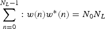 $\sum\limits_{n=0}^{N_{L} -1} : w\lpar n \rpar w^{\ast }\lpar n \rpar =N_{0} N_{L}$
is the noise power of NL samples with N0 is the power spectral density of noise. Then following analysis, similar to that in Equation (A5), leads to:
 $$\eqalign{ E\lcub {N_{w}^{2} } \rcub &\cong {C_{s} N_{0} \over \lpar {N_{L}}\rpar }\mathop \sum\limits_{k=0}^{T_{0} N-1} T_{s} \int\limits_{-\beta_{r} /2}^{\beta_{r} /2} {\sin^{2}\lpar {\pi fM_{k} T_{s} } \rpar \over \sin^{2}\lpar {\pi fT_{s} } \rpar }\lpar {1-\cos \lpar {2\pi f\!\!{\Delta }} \rpar } \rpar df \cr &= {2C_{s} N_{0} \over N_{L}} \sum\limits_{k=0}^{T_{0} N-1} \int\limits_{-\beta_{r} /2}^{\beta_{r} /2} G_{s_{k} } \lpar f \rpar \sin^{2}\lpar {\pi f\!\!{\Delta }} \rpar df}$$
Therefore, the variance of the signal error for a given t s is:
 $$var(e\lpar {t_{0} -t_{s}} \rpar \vert t_{s})\cong {C_{s}^{2} (K_{2} +K_{4} )^{2} \over 4}+{2C_{s} N_{0} \over N_{L} }\sum\limits_{k=0}^{T_{0} N-1} \mathop \smallint\limits_{-\beta_{r} /2}^{\beta_{r} /2} G_{s_{k} } \lpar f \rpar \sin^{2}\lpar {\pi f \Delta } \rpar df$$
From the coherent early-late TOA estimator block diagram, the unsmoothed TOA estimate is:
 $$t_{u} =t_{s} +{e\lpar {t_{0} -t_{s} } \rpar \over C_{s} K}$$
combining with Equations (B8) and (B9) the estimated range of the unsmoothed TOA is:
 $$t_{s} +{e\lpar {t_{0} -t_{s} } \rpar \over C_{s} K_{1} }\le t_{u} \le t_{s} +{e\lpar {t_{0} -t_{s} } \rpar \over C_{s} K_{3}}$$
mathematically, the conditional variance of t u for a given t s is:
 $$var(t_{u} \vert t_{s})={\sigma (e\lpar {t_{o} -t_{s} } \rpar \vert t_{s} ) \over C_{s}^{2} K^{2}}$$
The variance of the unsmoothed TOA estimator
 $\sigma_{u}^{2} $
, therefore, varies between
 $\sigma_{u1}^{2}$
and
 $\sigma _{u2}^{2}$
, where:
 $${\sigma_{u1}^{2}} =\sigma_{1}^{2} +\sigma_{u1N}^{2}$$
and
 $$\sigma_{u2}^{2} =\sigma_{2}^{2} +\sigma_{u2N}^{2}$$
in which
 $\sigma_{1}^{2}$
and
 $\sigma_{2}^{2}$
, which are respectively shown in Equations (18) and (19), are the DLL jitters that are influenced by the sampling frequency. Similarly,
 $\sigma_{u1N}^{2}$
and
 $\sigma_{u2N}^{2}$
, which are respectively illustrated in Equations (20) and (21), are the DLL tracking errors that are controlled by noise power.