3.1. Alignment Formula

Suppose that the latitude, the height and the ground velocity are known by survey or GPS, etc. The SINS alignment problem comes down to the unique determination of current attitude C _bⁿ using gyroscope and accelerometer outputs.

In order to obtain the analytic form of the current attitude matrix C _bⁿ, separately consider the attitude changes of the body frame and the navigation frame relative to some chosen inertial frame and then combine them together. By the chain rule of the attitude matrix, in this paper, C _bⁿ is decomposed as followed:

(3)$$C\hskip1pt_b^n (t) = C\hskip1pt_{n(t - m)}^{n(t)} C\hskip1pt_{b(t - m)}^{n(t - m)} C\hskip1pt_{b(t)}^{b(t - m)}, \quad m \gt 0$$

where C _b(t)^b(t−m) and C _n(t−m)^n(t) encode the attitude changes of the body frame and the navigation frame from time t−m to t respectively. It can be discovered that if the value m selects the whole length of the data, the decomposed form is exactly the same as the form in Silson (Reference Silson2011) and Wu and Pan (Reference Wu and Pan2013).

The rate equations of body and navigation frame respect to the inertial frame are:

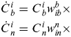(4)$$\eqalign{& \dot C\hskip1pt_b^i = C\hskip1pt_b^i w_{ib}^b \times \cr & \dot C\hskip1pt_n^i = C\hskip1pt_n^i w_{in}^n \times} $$

solutions to which are:

(5)$$C\hskip1pt_i^{bt} - C\hskip1pt_i^{bt - 1} = C\hskip1pt_i^{bt - 1} \cdot T \cdot w\hskip1pt_{ibt - 1}^b \times \Rightarrow C\hskip1pt_{bt - 1}^{bt} = I + T \cdot w\hskip1pt_{ibt - 1}^b \times \Rightarrow C\hskip1pt_{bt - m}^{bt} = C\hskip1pt_{bt - 1}^{bt} C\hskip1pt_{bt - m}^{bt - 1} $$

(6)$$C\hskip1pt_i^{nt} - C\hskip1pt_i^{nt - 1} = C\hskip1pt_i^{nt - 1} \cdot T \cdot w_{int - 1}^n \times \Rightarrow C\hskip1pt_{nt - 1}^{nt} = I + T \cdot w\hskip1pt_{int - 1}^n \times \Rightarrow C\hskip1pt_{nt - m}^{nt} = C\hskip1pt_{nt - 1}^{nt} C\hskip1pt_{nt - m}^{nt - 1} $$

The optimal approach in the references take the C _b(0)ⁿ⁽⁰⁾ as the initial attitude matrix, but here the C _b(t−m)^n(t−m) is the temporary initial attitude matrix. If the temporary initial attitude matrix C _b(t−m)^n(t−m), was known, the C _bⁿ(t) can be obtained by Equations (3), (4)and (5). So the method in this paper is called “a sliding optimization method for alignment based on inertial system”.

Then the most important value we have to obtain is the value of C _b(t−m)^n(t−m). Substituting Equation (3) into Equation (2) yields:

(7)$$\dot v^n = C\hskip1pt_{n(t - m)}^{n(\tau )} C\hskip1pt_{b(t - m)}^{n(t - m)} C\hskip1pt_{b(\tau )}^{b(t - m)} f^b - (2w_{ie}^n + w_{en}^n ) \times v^n + g^n, t - m \lt \tau \lt t$$

Multiplying C _n(τ)^n(t−m) on both sides,

(8)$$\hskip-6pt\eqalign{C\hskip1pt_{n(\tau )}^{n(t - m)} \dot v^n = & C\hskip1pt_{b(t - m)}^{n(t - m)} C\hskip1pt_{b(\tau )}^{b(t - m)} f^b - C\hskip1pt_{n(\tau )}^{n(t - m)} (2w_{ie}^n + w_{en}^n ) \times v^n + C\hskip1pt_{n(\tau )}^{n(t - m)} g^n \,,\,t - m \lt \tau \lt t} $$

Or equivalently,

(9)$$\eqalign{C\hskip1pt_{b(t - m)}^{n(t - m)} C\hskip1pt_{b(\tau )}^{b(t - m)} f^b & = C\hskip1pt_{n(\tau )}^{n(t - m)} \dot v^n + C\hskip1pt_{n(\tau )}^{n(t - m)} (2w_{ie}^n + w_{en}^n ) \times v^n - C\hskip1pt_{n(\tau )}^{n(t - m)} g^n, t - m \lt \tau \lt t} $$

Equation (9) forms the basis for the optimization approach, which could be readily applied to the alignment problem discussed in this paper if the velocity rate $\dot v^n$ was provided.

Integrating Equation (8) on both sides over the time interval of interest:

(10)$$\eqalign{ \int_{t - m}^t {C\hskip1pt_{n(\tau )}^{n(t - m)} \dot v^n} d\tau = &C\hskip1pt_{b(t - m)}^{n(t - m)} \int_{t - m}^t {C\hskip1pt_{b(\tau )}^{b(t - m)} f^b d\tau -} \int_{t - m}^t {C\hskip1pt_{n(\tau )}^{n(t - m)} (2w_{ie}^n + w_{en}^n )} \cr & \times v^n dt - \int_{t - m}^t {C\hskip1pt_{n(\tau )}^{n(t - m)} g^n d\tau}, t - m \lt \tau \lt t} $$

For the whole integration process in Equation (10), τ is the variable, the integrating range of the definite integral is the data segment between t−m moment to t moment, t and m are not the variables, so we can take the navigation frame of t−m moment as a kind of i-frame, so

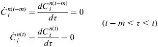(11)$$ \matrix{ {\dot C\hskip1pt_i^{n(t - m)} = \displaystyle{{dC\hskip1pt_i^{n(t - m)} } \over {d\tau }} = 0} \cr {\dot C\hskip1pt_i^{n(t)} = \displaystyle{{dC\hskip1pt_i^{n(t)} } \over {d\tau }} = 0} \cr } \quad\quad (t - m \lt \tau \lt t)$$

The left term of Equation (10) develops as

(12)$$\int_{t - m}^t {C\hskip1pt_{n(\tau )}^{n(t - m)} \dot v^n} d\tau = \int_{t - m}^t {\left( {C\hskip1pt_{n(\tau )}^{n(t - m)} v^n} \right){ \hskip-2pt\prime}} d\tau - \int_{t - m}^t {\dot C\hskip1pt_{n(\tau )}^{n(t - m)} v^n} d\tau $$

in which C _n(τ)^n(t−m) is the navigation frame of the moment τ with respect to the navigation frame of the moment t−m.

$$\dot C\hskip1pt_{n(\tau )}^{n(t - m)} = \left( {C\hskip1pt_i^{n(t - m)} C\hskip1pt_{n(\tau )}^i} \right) { \hskip-2pt\prime} = \dot C\hskip1pt_i^{n(t - m)} C\hskip1pt_{n(\tau )}^i + C\hskip1pt_i^{n(t - m)} \dot C\hskip1pt_{n(\tau )}^i $$

Combining Equations (12) and (4):

(13)$$\dot C\hskip1pt_{n(\tau )}^{n(t - m)} = C\hskip1pt_i^{n(t - m)} \dot C\hskip1pt_{n(\tau )}^i = C\hskip1pt_i^{n(t - m)} C\hskip1pt_{n(\tau )}^i w_{in}^n \times = C\hskip1pt_{n(\tau )}^{n(t - m)} w_{in}^n \times $$

Rewrite Equation (11):

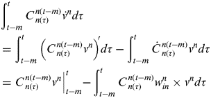(14)$$\eqalign{& \int_{t - m}^t {C\hskip1pt_{n(\tau )}^{n(t - m)} \dot v^n} d\tau \cr & = \int_{t - m}^t {\left( {C\hskip1pt_{n(\tau )}^{n(t - m)} v^n} \right){ \hskip-2pt\prime}} d\tau - \int_{t - m}^t {\dot C\hskip1pt_{n(\tau )}^{n(t - m)} v^n} d\tau \cr & = \left. {C\hskip1pt_{n(\tau )}^{n(t - m)} v^n} \right|_{t - m}^t - \int_{t - m}^t {C\hskip1pt_{n(\tau )}^{n(t - m)} w_{in}^n \times v^n} d\tau} $$

Substituting Equation (14) into Equation (10) and reorganizing the terms yields the velocity integration formula as

(15)$$C\hskip1pt_{b(t - m)}^{n(t - m)} \alpha _v = \beta _v $$

in which

(16)$$\eqalign{& \alpha _v \buildrel \Delta \over = \int_{t - m}^t {C\hskip1pt_{b(\tau )}^{b(t - m)} f^b d\tau} \cr & \beta _v \buildrel \Delta \over = \left. {(C\hskip1pt_{n(\tau )}^{n(t - m)} v^n )} \right|_{t - m}^t + \int_{t - m}^t {C\hskip1pt_{n(\tau )}^{n(t - m)} w_{ie}^n \times v^n} d\tau - \int_{t - m}^t {C\hskip1pt_{n(\tau )}^{n(t - m)} g^n d\tau}} $$

Note the four elements unit quaternion 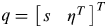$q = \left[ {\matrix{ s & {\eta ^T} \cr}} \right]^T $, where s is the scalar part and η is the vector part, is used to encode the initial body attitude matrix C _b(t−m)^n(t−m), the relationship between these two rotation parameters is:

(17)$$C\hskip1pt_{b(t - m)}^{n(t - m)} {\rm =} \unknown (s^2 - \eta ^T \eta )I + 2\eta \eta ^T - 2s(\eta \times )$$

Define the quaternion multiplication matrices by

$$\mathop {\left[ q \right]}\limits^ + \buildrel \Delta \over = \left[ {\matrix{ s & { - \eta ^T} \cr \eta & {sI + (\eta \times )} \cr}} \right], \quad \mathop {\left[ q \right]}\limits^ - \buildrel \Delta \over = \left[ {\matrix{ s & { - \eta ^T} \cr \eta & {sI - (\eta \times )} \cr}} \right]$$

Then Equation (15) is equivalent to $( {\mathop {[ \hskip1pt{\beta (t_M )} ]}\limits ^ + - \mathop {[ {\alpha (t_M )} ]}\limits^ -} )q = 0$, and the determination of the attitude quaternion can be posed as a constrained optimization

$$\mathop {\min} \limits_q q^T Kq , \quad {\rm subject \ to} \quad q^T \, q=1 $$

where the 4×4 real symmetric matrix

(18)$$K \buildrel \Delta \over = \sum\limits_M {( {\mathop {[ {\beta (t_M )} ]}\limits^ + - \mathop {[ {\alpha (t_M )} ]}\limits^ -} )^T ( {\mathop {[ {\beta (t_M )} ]}\limits^ + - \mathop {[ {\alpha (t_M )} ]}\limits^ -} )} $$

It can be proved that the optimal quaternion is exactly the normalized eigenvector of K belonging to the smallest eigenvalue.

Equation (15) is a fixed length integration function of the initial attitude matrix C _b(t−m)^n(t−m), with the two vectors α _v and β _v evidently defined in Equation (15). Note that α _v and β _v are respectively functions of the gyroscope/accelerometer outputs and the aided velocity/position information during the alignment period [0,t]. Theoretically, if there exist two linearly independent α _v or β _v, the initial attitude matrix C _bⁿ(t−m) for a fixed data segment can be uniquely determined, and further update the attitude matrix from the moment t−m to the moment t.

The value m is very important. Each time we get the C _bⁿ(t), the m length data segment from t−m to t must be used.

The optimal alignment is a method based on integrated form. The value m just represents the length of integral interval. If the value is big, the precision may deteriorate due to the integration of bias. If the value is small the precision may also be far from satisfied because the random noise requires quite a long data segment to obtain the required statistical characteristic.

3.2. Alignment algorithms implementation

The recursive algorithm is summarized below; note that the matrix K can be cursively computed using its previous value. Suppose T is the time interval indexed by k, the length of data for optimization is m, a constant value. The current time t=kT.

Initialization: set k = 0, Let C _b(t−m)^b(t) = C _n(t−m)^n(t) = I and K = 0_4×4

Step 1: set k=k+1

Step 2: Update C _b(kT−m)^b((k−1)T) to C _b(kT−m)^b(kT) using the gyroscope outputs w _ib^b, and C _n(kT−m)^n((k−1)T) to C _n(kT−m)^n(kT) using the w _inⁿ;

Step 3: Compute α(kT) and β(kT) using the accelerometer outputs f^band the velocity measurements. (see Equation (16))

Step 4: Update K((k−1)T) to K(kT) with the resultant α(kT) and β(kT) according to Equations (16) and (18)

$$K(kT) \approx \int_{kT - m}^{KT} {( {\mathop {[ {\hskip1.5pt\beta (t)} ]}\limits^ + \mathop { - [ {\alpha (t)} ]}\limits^ -} )^T ( {\mathop {[ {\beta (t)} ]}\limits^ + \mathop { - [ {\alpha (t)} ]}\limits^ -} )dt} ;$$

Step 5: Determine the initial attitude quaternion q by calculating the normalized eigenvector of K(kT) belonging to the smallest eigenvalue;

Step 6: Obtain the attitude matrix at current time using Equations (3) and (17);

Step 7: Go to Step 1 until the end.

4.1. The Simulation data

In this section, the validity of our algorithm and the influence of random and bias errors will be demonstrated. First, the conditions for the simulation are as follows: the true attitude is supposed to be (θ=−10°, γ=−20°, φ=−30°); the sampling frequency is 10 Hz; the longitude is 114·802° and latitude is 30·58°; the bias of the gyro is 0·01°/h, random noise is 0·01°/h; the bias of the accelerometer is 1×10⁻⁴ g, random noise is 1×10⁻⁵ g.

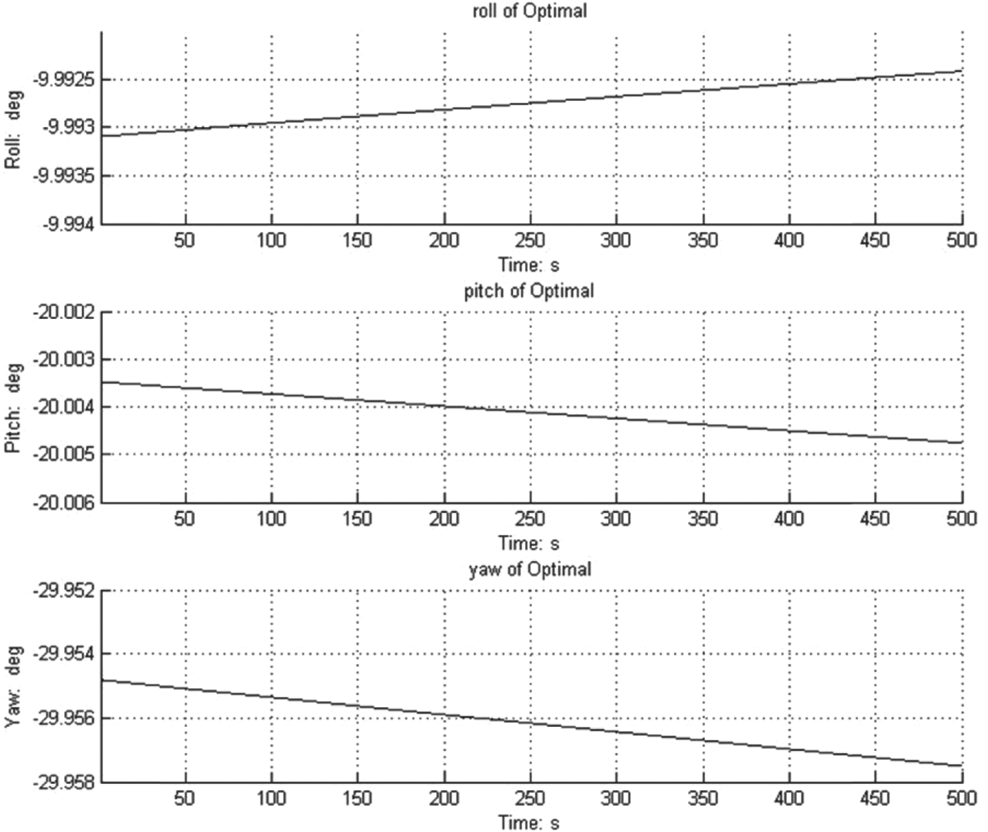
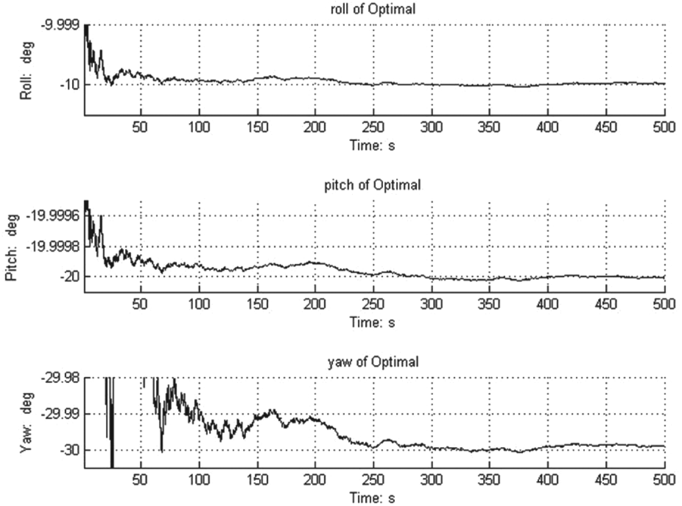
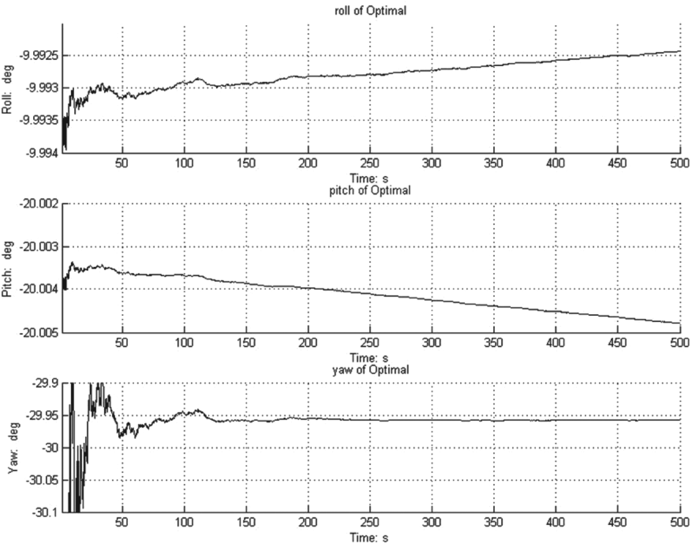
To illustrate the influence of the random noise and bias with the method in the reference clearly (Wu et al., Reference Wu, Wu, Hu and Hu2011), Figure 1 shows the alignment performance using the optimal alignment method under the circumstance that there is only bias in the simulation data. It can be seen that the bias makes a directional deviation to the alignment; the longer the data segment, the worse the deviation. Figure 2 shows the performance in the case of only random noise in the simulation data. It can be seen that random noise requires quite a long data segment to achieve alignment with almost no deviation. The alignment performance in the condition of the simulation data with both random noise and bias can be seen in Figure 3. This simulation data is regarded as the closest to true data. From Figures 1 to 3, we can conclude that the alignment requires a suitable length of data segment to restrain the influence of both random noise and bias.

Figure 1.

Simulation data with only bias.

Figure 2.

Simulation data with only random noise.

Figure 3.

Simulation data with random noise and bias.

4.2. The Measured Data

In the second supporting part, a piece of test data segment of the Fibre Optical Gyroscope (FOG) SINS was collected. The FOG SINS was installed on a double-axis turntable, as shown in Figure 4.

Figure 4(a).

IMU of FOG Strapdown INS.

Figure 4(b).

IMU on turntable.

In order to evaluate the accuracy of alignment we needed a criterion for comparison. Thus we ensured that the turntable had a highly accurate level through a level meter and an exact heading through an optical theodolite. 2000 s of static data from the FOG SINS was collected on the double-axis turntable.

The parameters were as follows: attitude of IMU was (θ = 0°, γ=0°, φ=36·8°). The length of the data was 2000 s, the sampling frequency was 10 Hz and the longitude and latitude were 114·802° and 30·58° respectively.

Figures 5 to 7 provide the attitude estimated by the method proposed with the test segment. Figure 5 shows the roll angle, Figure 6 shows the pitch angle, and Figure 7 shows the yaw angle.

Figure 5.

The optimal roll alignment.

Figure 6.

The optimal pitch alignment.

Figure 7.

The optimal yaw alignment.

Each figure has four curves, including the method in this paper when the value of m respectively is 10, 100, 1000, and the method proposed by the reference (Wu et al., Reference Wu, Wu, Hu and Hu2011). Through the figures we can see the curve of m=10 gives a high accuracy level, but a rather coarse heading. The curve of m=1000 shows a volatility in the level attitude. The curve of the method in the reference (Wu et al., Reference Wu, Wu, Hu and Hu2011) shows obvious flutter due to the integration over a long time from 0 to t. The curve of m=100 has a better performance.