Introduction
Astrobiology has several dissonances, but the most well-known is between the probability and evidence of extraterrestrial life. Detectability of extraterrestrial life is linked to the likelihood of its (un)correlated origin. Due to a synergy of physical limitations of life forms, the velocity of natural vehicles (solar and interstellar meteorites, comets), and physical conditions in interstellar space, the probability of observing correlated origin (i.e. dispersal origin) of extraterrestrial life decreases, even though the chance of finding it increases with the distance from the Earth. Abiogenesis, the spontaneous process through which non-viable matter becomes live organisms, appears to be the most plausible life origin mechanism on planets based on these factors (Wesson Reference Wesson2010).
Some conceptual studies ponder if standard, limiting definitions of life will prevent future astrobiological missions from identifying extraterrestrial life, and propose alternate definitions (Benner Reference Benner2010; Bartlett and Wong Reference Bartlett and Wong2020). In this light, we will summarize the basic intuitions (Bartlett and Wong Reference Bartlett and Wong2020) employed in our research rather than attempting to establish even a rudimentary definition of life: (1) Terrestrial life as we know it may be uncommon throughout the universe, but a universal class of entities with life-like attributes may be far more prevalent; (2) There may be entities that match the living characteristics better than even earthly life does, but they have yet to be discovered or even considered; (3) We can unravel knowledge and investigate the complete parameter space of physical and chemical interactions that may produce and propagate life by loosening limits on the notion of life.
Scientific evidence of life and its (un)correlated genesis, on the other hand, is expected to have mappable distributions throughout a wide range of spatial dimensions, from microscopic (<mm) to macroscopic (>AU) levels. Only probabilistic models, statistical representations that produce dependencies that allow inference and prediction between scales, can be used to examine this range of astrobiological scales (see Vukotić Reference Vukotić2010; Thompson et al. Reference Thompson, Candela, Wettergreen, Dobrea, Clark, Swayze, Clark and Greenberger2018; Chan et al. Reference Chan, Hinman, Potter-McIntyre, Schubert, Gillams and Awarmik2019).
Although biology shares some length-scale characteristics with chemistry and physics, it is distinct in that it is a dynamic science, as organisms and their lineages change dramatically over time. DNA transcription/replication can take anywhere from minutes to hours ($10^{-6}- 10^{-4}$ yr), whereas evolutionary change can take hundreds to thousands ($10^{3} - 10^{5}$
 ) of years, affecting organisms lineage.
In the context of life spreading on Galactic scales, cellular automata (CA) simulations are particularly noteworthy. In astrobiology, the use of probabilistic CA models was pioneered by Vukotić and Ćirković (Reference Vukotić and Ćirković2012), and followed by Hair and Hedman (Reference Hair and Hedman2013). Galera et al. (Reference Galera, Galanti and Kinouchi2019), recently, built a model based on an earlier study by Kinouchi (Reference Kinouchi2001). Djošović et al. (Reference Djošović, Vukotić and Ćirković2019) have also explored the relationship between spreading life and catastrophic processes in a similar discrete model.
The Galactic habitable zone and the circumstellar habitable zone (CHZ), postulated by Gonzalez et al. (Reference Gonzalez, Brownlee and Ward2001) and Lineweaver et al. (Reference Lineweaver, Fenner and Gibson2004) and formalized by Kasting et al. (Reference Kasting, Whitmire and Reynolds1993) distinguish regions in our Galaxy primarily on their levels of habitability. These ground-breaking studies paved the way for important discussions of correlations involved across the scales. Within these habitable zones, the spatial distribution of stars, exoplanets and exomoons differentiates these worlds according to the extent of habitability. When Heller and Armstrong (Reference Heller and Armstrong2014) considered which worlds might be more habitable than Earth, an interesting point went ahead. The authors propose that, just as the Solar System proved to be an outlier among planetary systems, Earth may prove to be an outlier among habitable or, eventually, inhabited worlds. As a result, it is possible that Earth is a planet with sub-optimal habitability compared to other superhabitable worlds. At the very least, compared to the equivalent regions of other stars, the solar CHZ may be a suboptimal location in our Galaxy. We still have a lot to learn about habitability, but similar to biogeography, we might be able to find clusters of habitable zones in some parts of our Galaxy where life can thrive. Any network of habitability zones that is eventually mapped may show dispersal routes or linkages between types of life that appear at nodes in the network. Such network analysis, for example, has been successfully utilized to investigate hydrothermal vent biogeography, as described by Moalic et al. (Reference Moalic, Desbruyéres, Duarte, Rozenfeld, Bachraty and Arnaud-Haond2012). Biogeography uses geographical and dispersion routes to explain species distribution. Gradual range dispersal, for example, is the continued transmission of populations by a series of conventional (short-distance) dispersal events, typically over extended time scales incorporating evolutionary processes. Jumping dispersal occurs when organisms overcome a barrier in a single, direct action rather than bouncing across ‘islands’. Sweepstakes routes are formed when organisms overcome a barrier unusually and dangerously, with just a few individuals surviving the journey (Ran Reference Ran2013).
Astrobiology may now examine some of the possible dispersal vectors and routes within the solar system thanks to advancements in space technology (see Kawaguchi Reference Kawaguchi2019, and references therein). Life spreading between planets in a single planetary system, such as the Solar System, would be considered as the short-range routes. Microscopic life could migrate between Earth and Mars, for example, via meteorites or comets, although this has yet to be verified. Melosh (Reference Melosh2003) determined that any rock ejected from a terrestrial planet in our Solar System will never collide with a similar terrestrial world in an exoplanetary system; in this view, short-range correlation effects are limited to the planetary system in question (Lingam and Loeb Reference Lingam and Loeb2017). Napier (Reference Napier2004), on the other hand, hypothesized that short-range correlation might have evolved into long-range correlation. It happens when meter-scale boulders blasted from Earth collide with other objects and dust particles in space, resulting in remains as small as a micron. These remnant particles can then be ejected from the Solar System as a result of radiation pressure.
The number of observations of interstellar objects traveling through our system has recently increased (e.g. Oumuamua asteroid and 2I$/$ Borisov comet Fitzsimmons et al. Reference Fitzsimmons, Snodgrass, Rozitis, Yang, Hyland, Seccull, Bannister, Fraser, Jedicke and Lacerda2018; Jewitt and Luu Reference Jewitt and Luu2019). Interstellar objects like these could be used to transport organic material between planetary systems. However, no microorganisms or fossils have yet been discovered in martian meteorites that have collided with Earth (Kerr Reference Kerr1997). Nonetheless, some research imply that life transmission is far more common in crowded environments. (see Belbruno et al. Reference Belbruno, Moro-Martín, Malhotra and Savransky2012).
Future and current space missions will aid in the investigation of these life-dispersal paths in our and exoplanetary systems, as well as in the regions of our Galaxy. If future investigations discover dispersal channels for life, it will have a significant impact on how future space life search initiatives are interpreted. Lin and Loeb (Reference Lin and Loeb2015) presented a novel observational approach for resolving this problem. The authors created a generic statistical strategy based on pandemic models on Earth that proposes that discovering biologically active planets within particular Galactic areas separated by regions where planetary life is rare or absent can be practically incontrovertible proof for life transmission.
Adams and Spergel (Reference Adams and Spergel2005), for example, examined the probability of life exchange in star-forming clusters, where exoplanetary systems are closer together and their relative speeds are lower. Zubrin (Reference Zubrin2020) has demonstrated that interactions between clouds of small bodies from approaching stellar systems could play a role in interstellar life exchange. Comets can be exchanged between stars due to gravitational disruption of these clouds. Furthermore, in young star clusters, an exchange of planets between systems can occur during their close encounters, which could be another pathway for interstellar life exchange (see Malmberg et al. Reference Malmberg, Davies and Heggie2011).
Ginsburg et al. (Reference Ginsburg, Lingam and Loeb2018) suggested that viruses, in addition to bacteria, may spread across the Milky Way. No biochemical derivatives such as methane or ${\rm N}_{2}{\rm O}$ should be detected remotely because viruses do not metabolize directly. However, understanding these alterations to Earth's biogeochemical cycles, the consequences of virus infection at an extraterrestrial ecosystem-level may be detectable (e.g. Berliner et al. Reference Berliner, Mochizuki and Stedman2018).
What we do know is that the high-profile infectious diseases (such SARS, H5N1, HIV, Ebola and COVID-19) show large-scale regional and temporal patterns, i.e. spatio-temporal clustering (Cliff and Ord Reference Cliff and Ord1981; Kirby et al. Reference Kirby, Delmelle and Eberth2017; Li et al. Reference Li, Pei, Chen, Song, Zhang, Yang and Shaman2020). At least three characteristics of interplanetary organic material transport and epidemic data are challenges to using traditional statistical methodologies. The data are rarely the result of planned experiments in both domains, the occurrences (observations) should not be independent, and the process is often only partially observable (Meyer et al. Reference Meyer, Held and Höhle2017). Surveillance technology in the field of astrobiology, however, has not yet reached its full potential.
Rather than considering unrelated events (where abiogenesis occurs with no relation to neighbouring regions), we investigate what to expect from a correlated life origin due to a ‘contagion’ hypothesis. We report on numerical tests carried out in the framework of a two-dimensional CA model for the local Galactic region.
The search for biosignatures with the European Extremely Large Telescope and space observatories (such as the James Webb Space Telescope (JWST, Gardner et al. Reference Gardner, Mather and Clampin2006) or Atmospheric Remote-sensing Exoplanet Large-survey Reference Tinetti, Drossart, Eccleston, Hartogh, Heske, Leconte, Micela, Ollivier, Pilbratt, Puig, Turrini, Vandenbussche, Wolkenberg, Beaulieu, Buchave, Ferus, Griffin, Guedel, Justtanont, Lagage, Machado, Malaguti, Min, Nørgaard-Nielsen, Rataj, Ray, Ribas, Swain, Szabo, Werner, Barstow, Burleigh, Cho, du Foresto, Coustenis, Decin, Encrenaz, Galand, Gillon, Helled, Morales, Muñoz, Moneti, Pagano, Pascale, Piccioni, Pinfield, Sarkar, Selsis, Tennyson, Triaud, Venot, Waldmann, Waltham, Wright, Amiaux, Auguères, Berthé, Bezawada, Bishop, Bowles, Coffey, Colomé, Crook, Crouzet, Da Peppo, Sanz, Focardi, Frericks, Hunt, Kohley, Middleton, Morgante, Ottensamer, Pace, Pearson, Stamper, Symonds, Rengel, Renotte, Ade, Affer, Alard, Allard, Altieri, André, Arena, Argyriou, Aylward, Baccani, Bakos, Banaszkiewicz, Barlow, Batista, Bellucci, Benatti, Bernardi, Bézard, Blecka, Bolmont, Bonfond, Bonito, Bonomo, Brucato, Brun, Bryson, Bujwan, Casewell, Charnay, Pestellini, Chen, Ciaravella, Claudi, Clédassou, Damasso, Damiano, Danielski, Deroo, Di Giorgio, Dominik, Doublier, Doyle, Doyon, Drummond, Duong, Eales, Edwards, Farina, Flaccomio, Fletcher, Forget, Fossey, Fränz, Fujii, García-Piquer, Gear, Geoffray, Gérard, Gesa, Gomez, Graczyk, Griffith, Grodent, Guarcello, Gustin, Hamano, Hargrave, Hello, Heng, Herrero, Hornstrup, Hubert, Ida, Ikoma, Iro, Irwin, Jarchow, Jaubert, Jones, Julien, Kameda, Kerschbaum, Kervella, Koskinen, Krijger, Krupp, Lafarga, Landini, Lellouch, Leto, Luntzer, Rank-Lüftinger, Maggio, Maldonado, Maillard, Mall, Marquette, Mathis, Maxted, Matsuo, Medvedev, Miguel, Minier, Morello, Mura, Narita, Nascimbeni, Nguyen Tong, Noce, Oliva, Palle, Palmer, Pancrazzi, Papageorgiou, Parmentier, Perger, Petralia, Pezzuto, Pierrehumbert, Pillitteri, Piotto, Pisano, Prisinzano, Radioti, Réess, Rezac, Rocchetto, Rosich, Sanna, Santerne, Savini, Scandariato, Sicardy, Sierra, Sindoni, Skup, Snellen, Sobiecki, Soret, Sozzetti, Stiepen, Strugarek, Taylor, Taylor, Terenzi, Tessenyi, Tsiaras, Tucker, Valencia, Vasisht, Vazan, Vilardell, Vinatier, Viti, Waters, Wawer, Wawrzaszek, Whitworth, Yung, Yurchenko, Osorio, Zellem, Zingales and Zwart2018 (Tinetti et al. Reference Tinetti, Drossart, Eccleston, Hartogh, Heske, Leconte, Micela, Ollivier, Pilbratt, Puig, Turrini, Vandenbussche, Wolkenberg, Beaulieu, Buchave, Ferus, Griffin, Guedel, Justtanont, Lagage, Machado, Malaguti, Min, Nørgaard-Nielsen, Rataj, Ray, Ribas, Swain, Szabo, Werner, Barstow, Burleigh, Cho, du Foresto, Coustenis, Decin, Encrenaz, Galand, Gillon, Helled, Morales, Muñoz, Moneti, Pagano, Pascale, Piccioni, Pinfield, Sarkar, Selsis, Tennyson, Triaud, Venot, Waldmann, Waltham, Wright, Amiaux, Auguères, Berthé, Bezawada, Bishop, Bowles, Coffey, Colomé, Crook, Crouzet, Da Peppo, Sanz, Focardi, Frericks, Hunt, Kohley, Middleton, Morgante, Ottensamer, Pace, Pearson, Stamper, Symonds, Rengel, Renotte, Ade, Affer, Alard, Allard, Altieri, André, Arena, Argyriou, Aylward, Baccani, Bakos, Banaszkiewicz, Barlow, Batista, Bellucci, Benatti, Bernardi, Bézard, Blecka, Bolmont, Bonfond, Bonito, Bonomo, Brucato, Brun, Bryson, Bujwan, Casewell, Charnay, Pestellini, Chen, Ciaravella, Claudi, Clédassou, Damasso, Damiano, Danielski, Deroo, Di Giorgio, Dominik, Doublier, Doyle, Doyon, Drummond, Duong, Eales, Edwards, Farina, Flaccomio, Fletcher, Forget, Fossey, Fränz, Fujii, García-Piquer, Gear, Geoffray, Gérard, Gesa, Gomez, Graczyk, Griffith, Grodent, Guarcello, Gustin, Hamano, Hargrave, Hello, Heng, Herrero, Hornstrup, Hubert, Ida, Ikoma, Iro, Irwin, Jarchow, Jaubert, Jones, Julien, Kameda, Kerschbaum, Kervella, Koskinen, Krijger, Krupp, Lafarga, Landini, Lellouch, Leto, Luntzer, Rank-Lüftinger, Maggio, Maldonado, Maillard, Mall, Marquette, Mathis, Maxted, Matsuo, Medvedev, Miguel, Minier, Morello, Mura, Narita, Nascimbeni, Nguyen Tong, Noce, Oliva, Palle, Palmer, Pancrazzi, Papageorgiou, Parmentier, Perger, Petralia, Pezzuto, Pierrehumbert, Pillitteri, Piotto, Pisano, Prisinzano, Radioti, Réess, Rezac, Rocchetto, Rosich, Sanna, Santerne, Savini, Scandariato, Sicardy, Sierra, Sindoni, Skup, Snellen, Sobiecki, Soret, Sozzetti, Stiepen, Strugarek, Taylor, Taylor, Terenzi, Tessenyi, Tsiaras, Tucker, Valencia, Vasisht, Vazan, Vilardell, Vinatier, Viti, Waters, Wawer, Wawrzaszek, Whitworth, Yung, Yurchenko, Osorio, Zellem, Zingales and Zwart2018) will initially be limited to the local region of our star system (i.e. within a few tens of light-years) due to technical constraints. Therefore, the CA model we present here concentrates on a straightforward life diffusion scenario within a small region of our Galaxy.
We aim to get a better understanding of life-diffusion within a Galactic patch by taking into consideration the spatial density and viable material mobility process. Furthermore, we want to establish how to decode phase space thresholds for extinction and persistence of life diffusion.
The following sections compose the content of this article. We discuss the statistical toy model for life spreading in the section Methods, which takes into account individual interactions among hosts in the galaxy patch by capturing viable material. Then, the section Results and Discussion analyses the numerical experiments and displays the phase space of life spreading as well as its properties. The key conclusions are summarized in the final section.
Methods
Instead of CA models considering the entire Galaxy, the CA we present here primarily considers a simple life diffusion scenario inside a small patch because the quest for biosignatures will initially only span a few tens of light-years beyond our system.
Here, we demonstrate how a SIR model (firstly introduced by Kermack and McKendrick Reference Kermack and McKendrick1927) implemented in a CA context can be used to simulate the dynamics of life diffusion. Kermack and McKendrick's work has been cited numerous times and has become a classic in infectious disease epidemiology (Breda et al. Reference Breda, Diekmann, de Graaf, Pugliese and Vermiglio2012). The papers of Kermack and McKendrick influenced the creation of mathematical models for disease spread in the 20th and 21st centuries, and they are still applicable in many epidemic circumstances (Carvalho and Gonçalves Reference Carvalho and Gonçalves2021).
CA parameters have been adjusted to account for Galactic patch characteristics while remaining compatible with SIR pandemic models. We separated the population of host systems into various habitability categories and maintained them through time using CA rules that are equivalent to non-linear ordinary differential equations:


The terms $S$ and $I$
 , respectively, denote the number of habitable and inhabited hosts. $R$
 is the total number of sterilized hosts. According to the first equation, an infected host ($I$
 ) can infect habitable ($S$
 ) neighbours at a rate of $b$
 . The second equation shows that hosts live for a length of time ${\rm \tau }_{lf}$
 before becoming sterilized ($R$
 ). At rate ${\rm \tau }_R$
 , a sterilized host becomes habitable again, according to the third equation. The above equations are defined at the time $t$
 and the spatial position $x$
 , such that $( t,\; \, x) \in [ 0,\; \, T] \times \Omega$
 , $\Omega$
 is a fixed and bounded domain in ${\mathbb R}\times {\mathbb R}$
 with smooth boundary $\partial \Omega$
 , and homogeneous Neumann boundary conditions ${\partial S\over \partial \eta } = {\partial I\over \partial \eta } = {\partial R \over \partial \eta } = 0$
 , where $\eta$
 is the outward unit normal vector on the boundary. The homogeneous Neumann boundary condition implies that the system described above is self-contained, and no emigration occurs beyond the boundary.
Our CA model for the Galactic patch includes a cluster of matter and voids, assuming Newtonian gravitational law. In a square lattice, we suppose that matter and emptiness are of equal size. CA cells can represent individual hosts as well as planetary systems or different stars due to the universal nature of transition rules. For the sake of simplicity, we will refer to them as hosts. As a result, the cell might represent a planetary system, a star or a void. The terms planetary system and star do not always refer to the singular objects that these terms typically signify.
CA is a 2D square lattice with $N\times N$ lattice cells and ${\cal T}$
 total time steps, with non-periodic boundary conditions (i.e. it has the topology of 2D squared field). It has matrix representation $CA^{l}\in R^{m\times m}$
 at each time step, with elements $ca^{l}_{ij},\; \, \, l \in {1,\; \, \cdots ,\; \, {\cal T}},\; \, i,\; \, j \in {1,\; \, \cdots ,\; \, m}$
 . Our CA is a four-state model, which means that each cell could only be in one of the four possible states. A lattice cell state is $ca^{k}_{ij} = 0$
 if there is a habitable host (i.e. planetary system) at the ith row and the jth column, or it is $ca^{k}_{ij} = 1$
 if it contains life, or it is $ca^{k}_{ij} = 2$
 if host is sterilized and finally it may be empty cell (void) $ca^{k}_{ij} = 3$
 . In a biological sense, the first and last states are passive, the second is active, whereas the third is just physically active. The number of neighbours, $n$
 , around a cell is calculated using the following equation: $n = ( 2\ast r + 1) ^2$
 where $r$
 is the range. We use a Moore Neighbourhood with a range of $r = 1$
 , which gives each cell eight possible neighbours. Further, we randomly populate the cells with hosts in the Galactic patch's initial state using the axisymmetric ansatz for stellar number density $n$
 (Zhu et al. Reference Zhu, Udalski, Novati, Chung, Jung, Ryu, Shin, Gould, Lee, Albrow, Yee, Han, Hwang, Cha, Kim, Kim, Kim, Kim, Lee, Park, Pogge, Poleski, Mróz, Pietrukowicz, Skowron, Szymański, KozLowski, Ulaczyk, Pawlak, Beichman, Bryden, Carey, Fausnaugh, Gaudi, Henderson, Shvartzvald and Wibking2017):

where $c\sim 1\, {\rm pc^{-3}}$ , $X,\; \, Y,\; \, Z$
 are galactocentric coordinates but for simplicity sake the third coordinate is taken as $Z = 0$
 .
The state transition for the cell at location $( i,\; \, j)$ at time step $k$
 is as follows: the habitable cell can be infected with life by an infected neighbour with an infection rate $b( t,\; \, d)$
 , where $t$
 and $d$
 represent time and distance, respectively. This rule is a state transition $0\rightarrow 1$
 . The host will bear life at a random constant rate $\tau _{lf}\in Rnd\{ 0,\; \, 0.05\}$
 ,where $Rnd$
 stands for randomly chosen value. A (pseudo) random numbers are generated using the Fast Mersenne Twister SFMT19937 generator (Saito and Matsumoto Reference Saito and Matsumoto2008), a high-quality generator with an exceptionally large period $2^{19937} - 1$
 or about $10^{6001}$
 of the produced sequence. A life -bearing cell can be sterilized by applying the (immunity) rate $g( t,\; \, d)$
 , which corresponds to a state transition $1\rightarrow 2$
 . We also account for the possibility of life recovering in the sterilized cell at varying rates $\tau _{lr}\in \{ 0.25,\; \, 0.5\}$
 . A state transition $2\rightarrow 1$
 corresponds to this scenario. The life recovery rate was included in the model only as a comparison to findings from macrofaunal diversity data, which show that all mass extinctions have a 10 Myr ‘speed rate’ in diversity recovery (Alroy Reference Alroy2008; Lowery and Fraass Reference Lowery and Fraass2019). However, unlike diversity, morphological complexity can be rebounded more quickly, reaching a plateau within $\sim 5$
 Myr following the Cretaceous mass extinction, as shown for planktic foraminifera (Lowery and Fraass Reference Lowery and Fraass2019). Furthermore, we let a life-terminated host become habitable again at a rate of $\tau _{R } = 0.2$
 , i.e. state transition $2\rightarrow 0$
 .
We regard the dispersion of matter content (e.g. dust, asteroids) or the presence of additional dispersal vectors as dynamic effects. As a result, we assumed that the infectious connections between CA cells are determined by a capture kernel: the rate at which viable material emanating from the host at location $l 1$ is captured at position $l 2$
 . The kernel can only be defined up to a proportionality constant, and we opt to have it in Gaussian form:

where $d$ is the Euclidean distance between the cells. We choose $p_{0} = 1$
 for the parameter $p_0$
 , which is infection probability at zero distance (i.e. when an infected cell is coincident with a habitable). ‘Optical depth of life spreading’ is controlled by the scale parameter $\sigma$
 , which governs the pace at which probability declines with distance. We let the parameter $\sigma$
 to be 50. Also, we assume that the temporal component of $b( t,\; \, d)$
 is periodic throughout time in our model:

where $\beta$ is a variable parameter, $t$
 is a time, and $P$
 is the infection period. We arbitrarily chose $P\sim 10\% {\cal T}$
 as a compromise between our ignorance and the possibility of substantial variability in such processes. For the immunity rate, we applied the following formula:

where $g_0$ represents a variable sterilizing rate. We set transmission of life for all events to be proportional to a parameter $b( t,\; \, d)$
 defining infection rate because both rate kernels $b( t,\; \, d)$
 and $g( d)$
 are proportional to $\kappa ( d)$
 . Then, utilizing simulations to arbitrary degrees of precision, the threshold value of $b$
 may be calculated numerically.
An average star of $1.3 M_{\odot }$ has a main sequence lifespan of around $\eta \sim 6\times 10^9$
 yr. In simulations, the star prototype was set at around $1.3\, M_{\odot }$
 . A ‘habstar’, or a star that is exceptionally hospitable to an Earth-like planet (Turnbull and Tarter Reference Turnbull and Tarter2003), is one way of describing a solar twin. Variability, mass, age, metallicity, and close companions are all factors examined while evaluating a habstar. The stipulation that the star is on the main sequence for at least 3 Gyr imposes an upper limit of $1.5\, M_{\odot }$
 , which corresponds to a hottest spectral type of F1 V (Turnbull and Tarter Reference Turnbull and Tarter2003). As a result, we assume that a star prototype is a viable Solar-like star with a mass that is closer to Copernican principle criteria and corresponds to the upper limit for habitable Solar-like systems ( i.e. $1.3\, M_{\odot }$
 ; Vukotić Reference Vukotić2010).
The time step of the evolution of CA is then specified by $\eta$ and ${\cal T}$
 , as follows $\eta /{\cal T} = 6\times 10^{9}/500\sim 12\times 10^6$
 yr. To compute an evolutionary sequence, we create an initial CA state by populating cells with stellar systems based on equation 4. We next infect 100 systems within the patch at random with life. This defines the lattice configuration at the initial time.
The simulations were run on the SUPERAST, HPE ProLiant DL380 Gen10 2x Xeon 4210-S 64GB SFF server located at the Department of Astronomy, Faculty of Mathematics, University of Belgrade (description in Kovačević et al. Reference Kovačević, Zeković, Ilić, Arbutina, Novaković, Onić, Marčeta and Djošović2021). There are two computational nodes in SUPERAST. Each node has 40 cores, 128GB RAM, 2TB memory on SSD, and 3 DP GFLOPS (DoublePrecision Giga Floating Point Operations Per Second). We developed the Python code for simulations and data presentations.
Results
The simulation results are presented in this section to assess the following topics: (i) characterizing general spatial patterns of feasible transfers; (ii) detecting emergent characteristics in the phase space given by simulation parameters. For the simulation, we employed a CA with $N = 10000$ cells dispersed in a $100\times 100$
 grid. The dynamics of SIR equations should, in theory, be insensitive to the population size N (Bittihn and Golestanian Reference Bittihn and Golestanian2020). Thus, for example, the spatio-temporal patterns of life spreading are not alternated by employing the CA with $200\times 200$
 cells. On the other hand, complex models will assume particular extra effects that alternate life-spreading properties locally (e.g. viable material speed) in such a way that invariance is destroyed (Bisin and Moro Reference Bisin and Moro2020).
Spatial patterns
Identifying observable spatial patterns is one of the critical problems about the propagation of viable material within the Galactic patch. There are two types of spatial patterns that might be explored in this context. As predicted by Lin and Loeb (Reference Lin and Loeb2015) stationary patterns would remain unaltered across time with intermittent zones of a high density of life-bearing hosts. On the other hand, we show here that spatio-temporal patterns that change over time might propagate like oscillatory waves or even turbulence.
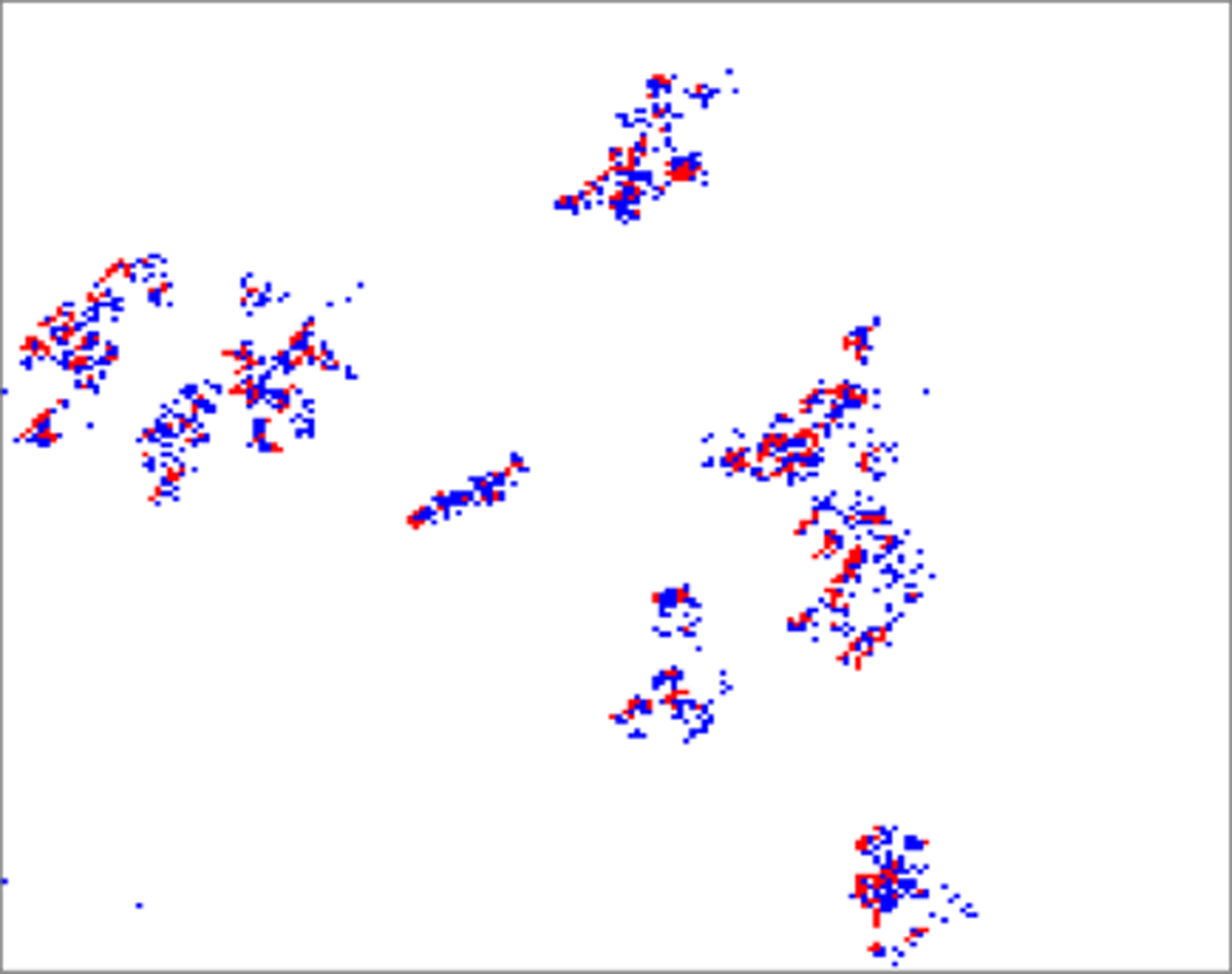
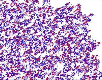
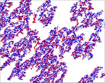
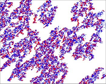
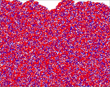
If hosts (e.g. planetary systems) are continuously distributed, life-dispersal spatial patterns can be best seen. Therefore, we assumed 100 randomly inhabited systems in such a grid. In Fig. 1 we exhibit several evolutionary sequences of continuously distributed hosts affected with life. The emerging states are formed either by an entanglement of clusters, ‘turbulences’ or ‘spiral waves’, characterizing the dynamics of the emergence of systems either infected with life, habitable or sterilized.
Spatial patterns in the life-diffusion network for various combinations of parameters when the distribution of hosts is homogeneous. Colours denote: white- homogeneous distribution of habitable hosts; red is life-bearing hosts and blue cells are life-terminated hosts. Upper row: Localized life outbreaks are self-limiting in size for $\beta = 0.62,\;$ at time instant $t = 4.6$
 (subplot a) but as time proceeds life-islands are still self-limited in size $t = 17$
 (subplot b). Middle: appearance of longer and narrow chains (waves) of life-outbreaks for $\beta = 1.2$
 , at time instant $t = 16$
 (subplot c), with time waves have tendency to connect $t = 21$
 (subplot d). Bottom: Stable spiral waves of life outbreaks (filaments) for $\beta = 2.75$
 at $t = 16$
 are broad (subplot e) and do not break with time $t = 20$
 (subplot f).

The parameter $\beta$ , which determines the life-spreading rate $b$
 , affects the spatial patterns. When the condition ($\beta = 0.62)$
 is met, the habitable (white) and inhabited (red) planets coexist in self-organized clusters of restricted size (Fig. 1, top left subplot). It indicates that isolated life outbreaks can fill in the lattice (right top subplot), but they can no longer expand; thus, they diminish and eventually vanish. When the $\beta$
 parameter is increased, the filaments of life-hosting structures grow in size and develop moving patterns (see ‘turbulence’ in the middle subplots and ‘spirals’ in the bottom subplots). The effectiveness of filling in the grid is the difference between two types of waves. Spirals are more effective in filling in the grid so that for a short period, they can populate the whole grid (bottom subplots). The interplay of the introduced CA rules sensitively determines whether life-bearing filaments can coexist on the grid or not. Whether or not life-bearing filaments may live on the grid is determined by the interaction of the introduced CA rules. We will go into more detail about stationary and moving patterns in the following subsection, focusing on conditions within phase space that allow for global extinction and persistence of life transmission as stationary patterns and transition between extinction and persistence as a moving spatio-temporal pattern.
Phase space of life transmission
In this part, we look at two different aspects of stationary and moving life-transmission patterns: (i) the features of life transmission phase spaces specified by model parameters $( b,\; \, g)$ and $( g,\; \, T)$
 ; (ii) the time it takes for life transmission to end in the Galactic patch, which provides information regarding life-spreading stability.
Extinction, persistence and transition
We are particularly interested in determining the phase transition between global termination and persistence of the life-spreading process, taking into account the distribution of planetary systems as described by equation (4). The global termination and persistence of the life-spreading process are both expressed as static spatial patterns. However, the transition between these two states has a spatiotemporal dynamic.
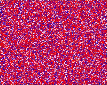
Figure 2 shows a random realization of an initial lattice. Due to the presence of voids, the dynamics of spreading are not obvious as they are in idealized circumstances (compare to Fig. 1).
CA with initial configuration of stellar systems sampled from density distribution given in equation (4). Red, green, blue and yellow stand for habitable, inhabited, sterilized planetary systems and voids between systems.

The phase transition between the persistence and extinction of life diffusion within the Galactic patch is determined via simulations. The interaction of sterilization and life infection rates defines this phase space ($g,\; b$ ). The perseverance part of phase space is defined as the region in which the spread of life will continue for the whole simulation run ${\cal T}$
 . The section of phase space where the life dispersal will terminate at any time instant $t< < {\cal T}$
 is called the termination part. The realizations of ($b,\; g$
 ) parameters space were calculated by simulating $100\times 100$
 cells lattice with 10 independent runnings. With time step 1, each run lasted 500 random time units. The lattice was initially set with a randomly chosen sample of planetary systems from a density distribution (equation (4)) at the start of each session. Then 100 planetary systems were chosen at random to be life-bearing.
Both $\beta$ and $g_0$
 , which were used to calculate the ($b,\; g$
 -plane, have values between 0.05 and 1.25, with an increase of $\Delta \beta = \Delta g_0 = 0.05$
 . After sterilization, the rate of life recovery is set to 0.25. We estimated a joint 2D probability density in ($b,\; g$
 ) phase space by averaging the results of all 10 independent runs (see Fig 3). The extinction zone (blue) is large, but the perseverance zone (yellow) is smaller and triangular in shape (left plot).
Average simulation realization of ($b,\; g$ ) phase space from 10 runs when the rate of life recovery after sterilization is 0.25. Left: The blue colour defines the termination part of phase space, and other colours stand for perseverance subregion. The yellow colour denotes that life-spreading continues during the whole period of simulation. Time is averaged and scaled. Right: The probability that the life spreading has gone extinct after a waiting time $t$
 when the g parameter is varied. Time is averaged but not scaled.

For a range of g between 0.5 and 1.25, typical waiting time ($T$ ) is often brief until life is terminated everywhere on the grid (blue region left plot). However, in $( g,\; \, T)$
 space, we discovered that the life spreading persists only for a limited range $g< 0.4$
 throughout the simulation (right plot). The likelihood of life spreading for a short time, on the other hand, is higher.
With a low probability, life can spread throughout intermediate periods (white dots in blue region). There are also phase space transition zones between extinction (blue region) and perseverance (yellow region), which are coloured with green and orange (left plot). Moreover, transition areas can occur with very low probability (left plot Fig. 3), which size is regulated by parameter $b$ .
The probability density function of the occurrence of habitable, inhabitable and life terminated hosts (planetary systems) for simulations presented in Fig. 3 is summarized in Fig. 4.
Probability density functions of habitable, inhabited and life-terminated planetary systems for simulation in Fig. 3. (a) Habitable hosts occupy almost whole phase space, except a tiny band for small b and larger g; (b) inhabited hosts are more probable to occur in the upper plateau (see right plot in Fig. 3); (c) life-terminated hosts are most likely to occur in lower plateau (compare to right plot in Fig. 3).

For parameter ranges $b< 0.5$ and $g> 0.45$
 , habitable hosts can occupy almost the whole phase space. Inhabited systems are more likely to exist in the zone specified by overall parameter $b$
 values except for $g> 1$
 , which is seen as the upper yellow region in the central plot of Fig. 4. When the parameter $b$
 is smallest and $g> 0.7$
 , life aborted hosts are most likely to occur near the bottom plateau, which is depicted as the yellow region in the right plot in Fig. 4.
The perseverance area of phase space (yellow) and transition section of phase space (green and orange) are expanded when the rate of life recovery is high $0.5$ (see the left plot in Fig 5). As a result, the typical waiting time $T$
 until life ends is usually significant.
The same as Fig. 3 but for the high rate of life recovery $0.5$ . Left plot: The blue colour defines the termination part of phase space, and other colours stand for perseverance subregion. The yellow colour denotes that life-spreading continued during the whole period of simulation. Time is averaged and scaled. The right plot is the probability that the life spreading has gone extinct after a waiting time $t$
 when the $g$
 parameter is varied, and the life recovery rate is high $\sim 0.5$
 . Time is averaged but not scaled.

The probability of life termination occurring early in simulation is extremely low (see the right plot in Fig. 5), as seen by the disappearance of the bottom plateau.
The probability density functions of occurrence of habitable, inhabitable and life terminated hosts are given in Fig. 6 for large values ($\sim 0.5$ ) of recovery rate of life. There are noticeable differences between Fig. 4, and Fig. 6. Habitable planets occur with a high probability (left panel) in more than half of phase space. However, the probability density space of inhabited hosts (middle panel) is slightly larger than for $b< 0.5$
 . A life-terminated system's probability density region is also slightly larger (right panel).
Probability density of habitable, inhabited and terminated systems for simulation in Fig. 5. From left to right: habitable systems occupy larger than a half of phase space; inhabitable systems are more probable to occur in the upper plateau (see the right plot in Fig. 5); terminated hosts are most likely bellow the upper plateau (compare to right plot in Fig. 5).

On the stability of life spreading
Through the simulations, when the parameter $b$ is larger, the waiting period $T$
 before life transmission is stopped can be quite long, but when $b< 0.5$
 , the waiting time is regulated by $g$
 (see Figs. 3 and 5). This shows that the waiting time $T$
 dependence on $g$
 is something to ponder carefully. When $b< 0.5$
 , the usual waiting time strongly increases as the ratio $T/g$
 approaches infinity in the asymptotic limit of small $g$
 . We can consider this arrangement to be stable for life spreading across the Galactic patch. If life recovery parameter $b$
 is smaller, the probability is high, as seen as an upper plateau, whose reflection in $( b,\; \, g)$
 phase space is shorter (see right plots in Fig. 3 and compare it to Fig. 5). When $T/g \rightarrow O( 1)$
 (i.e. the ratio approaches a finite non-zero value, see right plot in Fig. 3) a lower plateau appears, which can vanish completely when $b\geq 0.5$
 (see right plot in Fig. 5). It could be interpreted as a circumstance in which the life spreading is unstable, with a decreased probability. The third region with close to zero probabilities can occur anywhere between these two plateaus and is influenced by the $b$
 parameter (see left column of plots Figs. 3 and 5).
Discussion
Within a simulated Galactic patch, we discovered at least two probable spatial patterns of life transmission, corresponding either to stationary cluster patterns proposed by Lin and Loeb (Reference Lin and Loeb2015) or moving spatio-temporal patterns (in the form of waves or turbulences). The ‘speed’ with which the spatio-temporal patterns fill the spatial patch varies. The value of parameter $\beta$ , which determines the life-infection rate $b$
 , affects the diverse life-spreading spatial patterns. As $\beta$
 increases, the spatial forms of life transmission develop in size and form moving patterns of various speeds. The sterilization and life infection rates ($g,\; b$
 ) were used to create a phase space of life transmission. The CA simulations indicate the partitioning of phase space into two subregions: the perseverance subregion, where life diffusion will continue for $t = {\cal T}$
 , and the termination subregion, where life diffusion will come to a halt at substantially little time instants $t< < {\cal T}$
 . The third transition subregion is related to time instants progressively approaching the total simulation time ${\cal T}$
 . These phase space partitions are defined by the parameters $b$
 and $g$
 , as indicated. Larger values of $b$
 , for example, dramatically expand the phase space region where life can spread.
This statement is interesting, as it seems to be the opposite of what one would expect. In a given patch, the origin of life can be intrinsic abiogenesis or the ‘infection’ of the patch by panspermia. In either case, its probability is the site's inherent property and cannot relate to the independent probability of a catastrophe. For example, the life-terminating events could be non-local, e.g. SNe or $\gamma$ -ray bursts, affecting multiple habitable sites. In fact, by allowing greater flexibility, one can speculate that effects similar to those in the context of a metapopulation in biology (Chesson Reference Chesson2013) can take place. If the rate of extinction exceeds the rate of recolonization, the metapopulation as a whole will go extinct in the Galactic patch, and vice versa. Even if recolonization exceeds the extinction rate, there is a risk that metapopulations with only a few local populations will all go extinct simultaneously, resulting in the metapopulation's extinction (Chesson Reference Chesson2013). At any given period, catastrophic events in space must hit irregularly enough to wipe out only a part of local populations in the Galactic patch, or the metapopulation as a whole could perish (Chesson Reference Chesson2013). For example, environmental disturbance agents on our planet, such as fires and storms, are known to distribute death unevenly in space, despite their ability to affect a huge area in a short time (Chesson Reference Chesson2013). Still, as a result of climate change, catastrophic events are affecting much broader areas. Galactic patches may include two types of environment-disturbing agents: those that strike randomly and those that strike systematically. However, based on our simulations, it appears that the persistence of life spreading is impacted by the life-infection rate in irregular disasters.
For the self-formation of spatial patterns, the discrete character of the hosts involved in life-spreading mechanisms, as well as the transmission process rate, are critical.
We also observe that life transmission is sensitive to the rate of life recovery. The perseverance and transition parts of phase space are extended when the life recovery rate is large (0.5). This is because the time it takes for life to end in the Galactic region is usually significant. On the other hand transition zones (i.e. moving spatial patterns) can occur with very low probability when the rate of life recovery is lower (0.25). This parameter may vary from host to host, but we accounted for it as a constant for simplicity's sake. Because large-scale systems can have varying couplings among their components (Takeuchi et al. Reference Takeuchi, Chaté, Ginelli, Politi and Torcini2011), life-transfer observables on long-range temporal and spatial scales within the Galactic region are expected to be less resolvable than those on smaller scales, such as life spreading within a single planetary system.
The waiting time's dependency on $g$ appears to be critical to measure the stability of life-spreading mechanisms inside the patch under consideration. The ratio $T/g$
 is likely to approach an infinite or finite non-zero value. In the latter instance, there is a risk of life termination over the region due to instabilities in life transmission. The former could be interpreted as a scenario in which the spread of life is stable. Inter-species interactions such as competition, predation and symbiosis can define biodiversity within a region throughout life-spreading processes. However, because they can join to form a more extensive and complicated network of connections, these are not the only sorts of interactions. Species, on the other hand, can minimize competitive interaction and improve the chances of future colonization. Species can, for example, use alternate life dispersion methods that are usually encouraged by natural selection. This could be influenced by physical occurrences that provide an opportunity for non-competitive dispersal. The patterns may develop in size and eventually outgrow the system of natural hosts (i.e. planetary systems or planets) when the parameter $b$
 increases, as shown in the middle panel of Fig. 1. In the parameter space of larger values of $b$
 , life-bearing hosts may colonize another patch (see bottom panel of Fig. 1). We can not expect patches to be completely separated from one another if we assume the latter scenario. Finally, because life diffusion is disseminated mainly through vectors, the variables are naturally discontinuous and heterogeneously distributed. Larger and more sophisticated multi-patch settings will be the focus of our future research. We expect each patch to evolve separately through successive and varied forms of biotic forcing (colonization ability, reproduction, growth efficiency, dispersal capacityand other life strategies) according to the patch-mosaic model in biology. These processes promote the coexistence of a large number of species on much larger spatio-temporal scales (see Guilini et al. Reference Guilini, Soltwedel, van Oevelen and Vanreusel2011).
High levels of isolation, according to the biogeography of our planet, discriminate against dispersal. The loss of dispersal ability on oceanic islands, such as flightless birds (Carlquist Reference Carlquist1974), is an example of this.
Organisms in unique isolated habitats as subterranean caves, mountaintops, deep-sea trenches, thermal vents and hot springs pose reduced dispersal characteristics. Darwin (Reference Darwin1859) explained this phenomenon by counteracting selective forces acting before and after colonization of a remote island. Because of high-level isolation, species can lose their ability to disperse in just a few generations. Based on this, we can speculate that life forms on other planets can be either interplanetary dispersal-prone or -against depending on their host planet isolation (or level of possible material exchange in that region). We can hypothesize possible categories of interplanetary dispersal barriers based on various stresses organisms must endure: physiological, environmental or behavioural, environmental hazards, or behavioural difficulties in the environments they traverse.
In addition, dispersal barrier traversability can be classed as corridors, filters or sweepstakes, based on the complete range of probabilities of passing a barrier, from extremely probable to exceedingly improbable, respectively.(Simpson Reference Simpson1965). In densely packed planetary systems, such as the TRAPPIST-1 system, corridors may be formed. For example, three of seven planets are located within the HZ and have rocky compositions (Gillon et al. Reference Gillon, Jehin and Lederer2016, Reference Gillon, Triaud and Demory2017). Estimated orbital periods on the order of days, as well as orbital separations of $< 0.01$ AU, speed up material transfer between these planets, perhaps four to five times faster than between Earth and Mars (Lingam and Loeb Reference Lingam and Loeb2017; Krijt et al. Reference Krijt, Bowling, Lyons and Ciesla2017). For solar-like planetary systems and cosmic regions akin to the solar neighbourhood, filters and sweepstakes (extremely improbable transmission pathways) would be beneficial.
On our planet, life recovery happens after each mass extinction as correlated events (Newman and Eble Reference Newman and Eble1999; Newman and Palmer 2003), but with non-uniform ‘speed’. One can imagine a context in which violent events in synergy with spatial patterns in Galactic patches can induce selection for ‘the rate’ of life recovery and spread, similar to what we know about different speeds of diversity and complexity recovery after the Permian-Triassic (PT) catastrophe (Song et al. Reference Song, Wignall and Dunhill2018). Violent global regulatory mechanisms can be supernova explosions that have been first discussed as such by Vukotić (Reference Vukotić2010), while local ones comprise meteor impacts, volcanism and chemical compositions. For instance, according to Newman and Eble (Reference Newman and Eble1999) extinctions on Earth at various times are correlated, and extinctions within a single stage are not independent events. Newman and Palmer (2003) examined the number of families of marine animals that appeared with the number that went extinct in each geological stage since the Phanerozoic began and found that there are origination peaks that match all of the significant extinction peaks. However, there is no perfect correlation between the two curves characterizing these two sorts of events. Moreover, on our planet, different aspects of life recovery do not occur at the same time. There is a distinction to be made between diversity and complexity recovery. For example, nearly all life on Earth was wiped around 252 million years ago during Earth's largest mass extinction (Sepkoski Reference Sepkoski1984), known as the PT mass extinction, named after the two geologic periods it delineates. The recovery of marine ecosystems is thought to have taken several million years (Erwin Reference Erwin1998), with gradual recovery from the bottom to the top trophic levels (Chen and Benton Reference Chen and Benton2012). However, data imply (Song et al. Reference Song, Wignall and Dunhill2018) that the restoration of the marine ecosystem ($\sim 50$ Myr) took an order of magnitude longer than the recovery of biological diversity($\sim 5$
 Myr).
In the same way that a synergy of mechanisms controls the evolution of life forms on our planet, a synergy of mechanisms may exist to govern the evolution of life forms that cause relatively moderate but frequent life recovery and spread after each reset of life on a planet or planetary system. Individual life forms migrate over space, which is a critical element of Earth's ecosystems. Migration may also be a key competitor with local planetary interactions within the Galactic patch, thereby influencing species preservation and biodiversity.
The parameters $b$ and $g$
 could be generalized functions that include interplanetary system covariates such as observable biological, chemical or other environmental characteristics. It is also feasible to add data, either in a static sense, where the distance kernel may allow for material exchange direction or in a dynamic sense, where the kernel could alter over time as new exoplanet data become available. The phase space of life spreading can thus be recreated using the biomarkers and biosignatures data from a specific Galaxy patch. It is critical to understand that these spatially heterogeneous reactions might modify transmission patterns in unexpected ways. As a result, in order to qualitatively explain these findings, thorough knowledge is still required, which could lead to additional research.
According to the recent study by Totani (Reference Totani2020) the predicted number of abiogenesis events for a star, galaxy or perhaps the entire observable universe is $< 1$ . Because the volume of the observable universe is $< 10^{-78}$
 of the total inflation universe, Totani (Reference Totani2020) suggested that it is impossible to predict more than one abiogenesis event in such a small location without sufficient evidence. Even if Earth were the only planet with life within the observable universe, life could nonetheless emerge on innumerable planets throughout the inflationary cosmos. If abiogenesis is the only process for the origination of life everywhere, Totani (Reference Totani2020) calculations demonstrate that detecting non-terrestrial biosignatures in Solar and extraterrestrial systems will be extremely improbable.
Totani's analysis has some strong counterarguments. First, although the early Big Bang's inflation episode provides elegant solutions to some observable universe dilemmas, it has significant difficulty explaining how the inflation process began and ended. Iijas et al. (Reference Iijas, Loeb and Steinhardt2013); Iijas et al. (Reference Iijas, Steinhardt and Loeb2014) and Ijjas and Steinhardt (Reference Ijjas and Steinhardt2016) demonstrated that Planck satellite data ruled out the simplest inflation models and that the remaining inflation models necessitate more parameters, fine-tuning and more improbable initial conditions. At the very least, it appears that the inflation theory will need to be extensively revised, while numerous suggested changes do not appear to impact Totani's main conclusion. Second, Totani's research is limited to carbon-based biology (RNA-based biology). However, while other elements may be used to create live organisms, carbon-based biochemistry is widely acknowledged as the most ideal for producing complex molecules, which is essential for any possible kind of living or sentient beings. Finally, while Totani's analysis is based on current research, it is still vulnerable to future laboratory tests of the RNA world hypothesis. If extraterrestrial species of a different origin than those on Earth are discovered in the future, it will imply an unknown mechanism at work to polymerize nucleotides considerably quicker than random statistical processes, as Totani himself points out.
However, if interplanetary and (or) interstellar transmission of viable material is allowed (Nicholson Reference Nicholson2009; Wesson Reference Wesson2010) life detection elsewhere is more likely to occur. In seminal works such as Zuckerman (Reference Zuckerman1985) and Ćirković and Bradbury (Reference Ćirković and Bradbury2006) various plausible motivations for life migrations have been found.
Nonetheless, certain violent events may indirectly improve life transmission. The presence of the supermassive black hole at the Galactic core, for example, might result in a large flux of ionizing radiation, causing planetary atmospheric erosion and possibly severe consequences on surface life (Wisłocka et al. Reference Wisłocka, Kovačević and Balbi2019). At the same time, erosion effects could have increased the number of terrestrial planets formed from a gaseous envelope of sub-Neptune planets (Chen et al. Reference Chen, Forbes and Loeb2018), or stimulated prebiotic chemistry or even photosynthetic activity on planets without incoming radiation (Lingam et al. Reference Lingam, Ginsburg and Bialy2019).
If life can be transmitted across stellar systems, the highest rate of catastrophic events could be mitigated by the possibility that life can relocate swiftly to safer areas (Balbi et al. Reference Balbi, Hami and Kovačević2020) or that life recovery rate is high within denser Galactic regions like the bulge.
The phase volume within which life diffusion occurs is the multidimensional space, determined by mass–viable transfer–extinction interactions, wherein life can exist. This phase space represents an emergent property informed by all levels of interactions and the laws of thermodynamics. Indeed, specific neighbourhood systems are just one point within this space. The phase space, as we have seen, can increase or decrease depending on assumed interactions. We believe there is a concentration gradient, so the material will predominantly move from high to low concentration regions in the Galactic patch. The phase space itself may have its gradient defined by the ability of life diffusion to overcome the threshold imposed by parameter $b$ , leading to an increase or a decline in diversity.
Conclusion
The availability of biosignatures from planned ground and space surveys will allow precise measurement of phase-space as the ‘standard’ for understanding life-spreading mechanisms.
According to our results, we identify three qualitatively different phase space regions in terms of possible interstellar life-spreading outcomes based on transmission and sterilization parameters: perseverance, extinction and transition zone. Based on our simulations, the size of these three regions is apparently governed by infection rate (parameter $b$ ). Thus, three possible geometrical shapes (‘waves’) of interstellar life spreading have been identified. Finally, our results suggest the sensitivity of interstellar life-transmission processes by revealing how small changes in the parameters can cause changes in population-level outcomes such as the probability density of inhabited and sterilized hosts (planetary systems). Though proposing a generative mechanism for life-transmission is beyond the scope of this research, our work brings a new piece to the puzzle of (un)correlated life-origin.
Acknowledgments
The reviewers have provided extremely detailed and useful suggestions regarding the text clarity and presentation, for which we are grateful. The author acknowledge funding provided by the Faculty of Mathematics University of Belgrade (the contract 451-03-68/2020-14/200104), through the grants by the Ministry of Education, Science, and Technological Development of the Republic of Serbia. A.K. acknowledges the support by Chinese Academy of Sciences President's International Fellowship Initiative (PIFI) for visiting scientist. A part of this work has been presented as a short oral presentation at the Europlanet Science Congress (Virtual meeting) 2020.