1 Introduction
Numerous studies support the idea that wavepackets, obtained as linear stability solutions with the mean velocity field as a base flow, dominate at least the low-angle sound radiation (Jordan & Colonius Reference Jordan and Colonius2013) of subsonic turbulent jets. The structure of the sound field is consistent with a wavepacket source at low emission angles (Cavalieri et al.
Reference Cavalieri, Jordan, Colonius and Gervais2012), and wavepackets educed from data in the hydrodynamic region agree closely with linear theory in regions upstream of the end of the potential core and over a broad range of Strouhal numbers (Cavalieri et al.
Reference Cavalieri, Rodriguez, Jordan, Colonius and Gervais2013). The agreement is, however, poor in all regions at Strouhal numbers below
 $St=0.3$
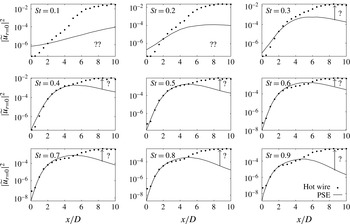
, and downstream of the end of the potential core for all Strouhal numbers (see figure 1). Moreover, noise predictions by such linear wavepacket models are orders of magnitude lower than experimental results (Jordan et al.
Reference Jordan, Colonius, Brès, Zhang, Towne and Lele2014; Zhang et al.
Reference Zhang, Jordan, Lehnasch, Cavalieri and Agarwal2014). Two-point coherence is another quantity that linear models cannot model correctly (Cavalieri & Agarwal Reference Cavalieri and Agarwal2014; Baqui et al.
Reference Baqui, Agarwal, Cavalieri and Sinayoko2015). These discrepancies are all believed to be due to a dynamic trait of wavepackets, related to nonlinearities, and which has been designated as jitter. The early study of Ffowcs-Williams & Kempton (Reference Ffowcs-Williams and Kempton1978) showed that jitter of wavepackets might significantly increase the associated sound radiation, and recent studies have confirmed its importance for obtaining quantitatively accurate noise prediction (Cavalieri et al.
Reference Cavalieri, Jordan, Agarwal and Gervais2011b
; Kerhervé et al.
Reference Kerhervé, Jordan, Cavalieri, Delville, Bogey and Juvé2012; Jordan et al.
Reference Jordan, Colonius, Brès, Zhang, Towne and Lele2014; Baqui et al.
Reference Baqui, Agarwal, Cavalieri and Sinayoko2015).
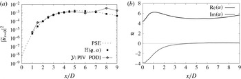
Measured streamwise velocity fluctuation on the jet centreline (circles) from Cavalieri et al. (Reference Cavalieri, Rodriguez, Jordan, Colonius and Gervais2013) and the results of PSE (line).

A simplified dynamical model, which attempts to account for this behaviour by implicitly incorporating nonlinearity via an unsteady base flow, was recently tested by Jordan et al. (Reference Jordan, Colonius, Brès, Zhang, Towne and Lele2014) and Zhang et al. (Reference Zhang, Jordan, Lehnasch, Cavalieri and Agarwal2014). The model produced jittering wavepackets with considerably enhanced sound radiation, but it was found that the noise increase was not sufficient to explain the observed levels. It appears, therefore, that nonlinearity must be accounted for in a more complete manner.
In this work, we consider the nonlinearity – which can be rigourously expressed via generalised Reynolds stresses – as an ‘external’ forcing, and we focus on its influence on wavepackets by studying the flow response to such forcing. Such a framework was first envisaged by Landahl (Reference Landahl1967), and has recently been applied to wall-bounded flows by McKeon & Sharma (Reference Mckeon and Sharma2010) and Sharma & McKeon (Reference Sharma and Mckeon2013) and to a backward facing step by Beneddine et al. (Reference Beneddine, Sipp, Arnault, Dandois and Lesshafft2016). The jets here considered issue from nozzles with turbulent boundary layers, and hence comprise a broad range of frequencies and wavenumbers. Among the relevant turbulence structures, wavepackets play a dominant role in sound radiation, but they are not isolated from other structures. We consider here the simplified scenario of one-way interaction, where the background turbulence affects the evolution of wavepackets via nonlinear interactions, but we do not study the effect of wavepackets on the nonlinear term; it is this assumption that enables the interpretation of turbulence as an ‘external forcing’.
In linear stability analysis of inviscid parallel shear flows, the critical layer, defined as that transverse location at which the phase speed of a wave is equal to the local speed of the base flow, gives rise to a singularity (Lin Reference Lin1954; Huerre Reference Huerre1980; Huerre & Scott Reference Huerre and Scott1980; Maslowe Reference Maslowe1986; Cowley & Wu Reference Cowley and Wu1994). When studying the transition of such flows, the critical-layer singularity is usually overcome by considering either viscous or nonlinear effects in the evolution of instabilities (Haberman Reference Haberman1976); both effects produce significant effects even when present at low amplitudes. In this work, we are in a different situation, as we study the evolution of wavepackets immersed in a turbulent flow, as described above. It is therefore more appropriate to consider the response of wavepackets to external forcing, and the physical interpretation of what happens at the critical layer is different from that which would be usual in laminar–turbulent transition. For wavepackets in turbulence, the key behaviour involves an increased sensitivity of the former to the latter when the growth rates of the former become weak, favouring a transition from modal to non-modal evolution.
A resolvent analysis is first considered. It involves a consideration of the flow in terms of the operator that is obtained by linearisation about the turbulent mean. This framework permits a forcing–response (or input–output) type interpretation, where the nonlinear terms are the forcing (input), and the linear waves supported by the operator are the response (output). Optimal harmonic forcing and associated responses are obtained by performing singular value decomposition of the resolvent of the linearised Navier–Stokes operator. This non-modal stability technique has been applied by Sharma & McKeon (Reference Sharma and Mckeon2013) to model coherent structures in turbulent pipe flow and has been considered in the context of the critical-layer mechanism by McKeon & Sharma (Reference Mckeon and Sharma2010). The method has been applied recently for a number of amplifier flows (globally stable flows, which can present spatial amplification of incoming disturbances): a backward facing step has been studied in a global setting by Dergham, Sipp & Robinet (Reference Dergham, Sipp and Robinet2013), who showed the link between harmonic and stochastic forcing analyses; Garnaud et al. (Reference Garnaud, Lesshafft, Schmid and Huerre2013), Nichols & Jovanović (Reference Nichols and Jovanović2014), Jeun, Nichols & Jovanović (Reference Jeun, Nichols and Jovanović2016) and Semeraro et al. (Reference Semeraro, Jaunet, Jordan, Cavalieri and Lesshafft2016) also considered a global approach to explore the amplifier character of jets. In our study, we adopt a locally parallel framework. In addition to the computational ease in comparison with global analysis, the local analysis serves as a complementary tool, providing insight regarding the local mechanisms (Lesshafft Reference Lesshafft2015) and supporting the interpretation of results obtained in the second study where non-parallel effects are permitted. Specifically, optimal response modes (forced wavepackets) and optimal forcing modes (the modes through which nonlinear interactions force wavepackets) are thus computed in different regions of the jet and compared with linear wavepacket results and experimental data for a Mach 0.4 jet, which has been examined in several previous studies (Cavalieri et al. Reference Cavalieri, Jordan, Colonius and Gervais2012, Reference Cavalieri, Rodriguez, Jordan, Colonius and Gervais2013; Baqui et al. Reference Baqui, Agarwal, Cavalieri and Sinayoko2015).
By means of a non-parallel approach, 4D variational data assimilation (4D-Var), we solve the input–output problem in an inverse manner by searching for the optimal forcing profile giving rise to improved agreement between flow response, obtained as solutions of the forced parabolised stability equation (PSE) system, and measurements. The approach allows us to identify the pieces that are missing in the linear model and whose addition would enable accurate prediction of the observed wavepacket behaviour. The 4D-Var technique is data driven in nature and has been used extensively in weather forecasting (Navon Reference Navon2009) to combine different sources of inhomogeneous information: a simplified model, noisy and sparse observations, and an a priori knowledge of the solution. It has also evolved as a powerful flow-control technique (Cordier et al. Reference Cordier, Noack, Daviller, Tissot, Lehnasch, Delville, Balajewicz and Niven2013). We introduce a novel use of this method for wavepacket modelling, in a slowly diverging base flow using the PSE; we thus avoid the locally parallel assumption. Interpretation of the results obtained is considerably aided by the results of the locally parallel analysis. We exploit the versatility of 4D-Var in order to gain insight on how different forcings affect wavepackets. We first determine the sensitivity of wavepackets to external forcing; this sensitivity analysis can be compared with the results of the resolvent analysis. In a second step, we compute optimal infinitesimal forcings, where optimality is in the sense of minimisation of the error between model and experiment; this analysis allows us to identify forcing terms that are lacking in standard linear wavepacket models. Finally, with such forcings we perform the optimisation and obtain the minimal forcing that produces wavepackets that match the experimental measurements.
The paper is organised as follows. In § 2, we introduce the framework, which consists of considering the harmonic external forcing as Fourier components of the nonlinear terms in the Navier–Stokes equations. In § 3, we present the locally parallel resolvent analysis. In § 4, we show the PSE-4D-Var approach. Finally, in § 5, we conclude the paper with a discussion of the results and some perspectives.
2 Nonlinear effects as external forcing
In what follows, we recall earlier results (Cavalieri et al.
Reference Cavalieri, Rodriguez, Jordan, Colonius and Gervais2013) where a detailed comparison between linear wavepacket models and experimental results was performed for a turbulent subsonic jet of Mach number
 $M=0.4$
. Extensive measurements were taken which allowed Fourier decomposition of velocity and (near- and far-field) pressure fluctuations into azimuthal wavenumbers and frequencies (expressed in terms of the Strouhal number,
 $St=fD/U$
, where
 $f$
is the frequency,
 $D$
is the jet diameter and
 $U$
is the jet exit velocity). The space variable is
 $\boldsymbol{x}=(x,r,\unicode[STIX]{x1D703})$
, where
 $x$
is the downstream distance from the nozzle exit,
 $r$
is the radius measured from the jet axis and
 $\unicode[STIX]{x1D703}$
is the azimuthal angle. The Reynolds number,
 $Re=\unicode[STIX]{x1D70C}UD/\unicode[STIX]{x1D707}$
, is equal to
 $4.2\times 10^{5}$
, where
 $\unicode[STIX]{x1D70C}$
and
 $\unicode[STIX]{x1D707}$
are reference density and dynamic viscosity values, taken at the nozzle exit. The boundary layer inside the nozzle is tripped, and measurements show that it is turbulent; hence, we consider the jet as turbulent from the outset. A more complete description of the experimental set-up and measurements can be found in Cavalieri et al. (Reference Cavalieri, Rodriguez, Jordan, Colonius and Gervais2013). The variables of the compressible equations are non-dimensionalised using the jet diameter, the ambient speed of sound and thermodynamic variables.
The spatial evolution of wavepackets, resulting from the well-known Kelvin–Helmholtz instability of the turbulent mean flow, is well predicted by linear models (Jordan & Colonius Reference Jordan and Colonius2013), such as linear PSE, for a wide range of frequencies until approximately the end of the potential core. Throughout this work we focus on the axisymmetric mode (
 $m=0$
, where
 $m$
is the azimuthal wavenumber), which is the most acoustically efficient (Cavalieri et al.
Reference Cavalieri, Rodriguez, Jordan, Colonius and Gervais2013). Figure 1 summarises a comparison (Cavalieri et al.
Reference Cavalieri, Rodriguez, Jordan, Colonius and Gervais2013) between the linear PSE and the Fourier component of hot-wire measurements of axial velocity fluctuations
 $\tilde{u}$
on the centreline of an
 $M=0.4$
jet, with Strouhal numbers,
 $St$
, ranging from
 $0.1$
to
 $0.9$
. Good agreement is observed for
 $St$
higher than
 $0.3$
, for the spatial amplification from the nozzle exit (
 $x=0$
) up to the end of the potential core (
 $x\approx 5D$
). Beyond the potential core, due to the spreading of the jet, the linear model predicts a decay. However, experiments (Cavalieri et al.
Reference Cavalieri, Rodriguez, Jordan, Colonius and Gervais2013) show an increase of the amplitude of the axisymmetric wavepacket on the centreline. Similar discrepancies between the linear model and experiment are observed in the near pressure field (Gudmundsson & Colonius Reference Gudmundsson and Colonius2011; Breakey et al.
Reference Breakey, Jordan, Cavalieri, Léon, Zhang, Lehnasch, Colonius and Rodriguez2013). For Strouhal numbers of
 $0.1$
and
 $0.2$
, the agreement in amplitudes, as seen in figure 1, is not good; comparison of phases shows better agreement even for these lower values of
 $St$
(Gudmundsson & Colonius Reference Gudmundsson and Colonius2011). This low-Strouhal behaviour is not considered here; we focus on wavepackets for values of
 $St$
above
 $0.3$
. In order to accurately model wavepackets throughout the flow, the linear model is clearly not sufficient and nonlinearities must be incorporated in some way; this is particularly relevant where sound radiation of subsonic jets is concerned, as discussed by Cavalieri & Agarwal (Reference Cavalieri and Agarwal2014), Jordan et al. (Reference Jordan, Colonius, Brès, Zhang, Towne and Lele2014) and Baqui et al. (Reference Baqui, Agarwal, Cavalieri and Sinayoko2015). We have chosen in this paper to consider nonlinear effects on the wavepacket as a harmonic forcing.
For the flow variable,
 $\boldsymbol{q}_{\unicode[STIX]{x1D719}}=(\boldsymbol{u},T,\unicode[STIX]{x1D70C})$
, containing the
 $N_{c}$
components of velocity, temperature and density, we consider the Reynolds decomposition,
 $\boldsymbol{q}_{\unicode[STIX]{x1D719}}(\boldsymbol{x},t)=\bar{\boldsymbol{q}}(\boldsymbol{x})+\boldsymbol{q}^{\prime }(\boldsymbol{x},t)$
, where
 $\bar{\boldsymbol{q}}(\boldsymbol{x})$
is the mean flow and
 $\boldsymbol{q}^{\prime }(\boldsymbol{x},t)$
is the fluctuation;
 $t$
is the non-dimensional time. For a jet, using homogeneity in the azimuthal direction, we decompose the fluctuation into Fourier modes,
 $$\begin{eqnarray}\displaystyle \boldsymbol{q}^{\prime }(x,r,\unicode[STIX]{x1D703},t)=\frac{1}{(2\unicode[STIX]{x03C0})^{2}}\mathop{\sum }_{m}\int _{-\infty }^{\infty }\widetilde{\boldsymbol{q}}_{\unicode[STIX]{x1D714},m}(x,r)\text{e}^{\text{i}(m\unicode[STIX]{x1D703}-\unicode[STIX]{x1D714}t)}\,\text{d}\unicode[STIX]{x1D714}. & & \displaystyle\end{eqnarray}$$
Introducing decomposition (2.1) in the Navier–Stokes (NS) equations, we obtain, in operator notation,
 $$\begin{eqnarray}\displaystyle {\mathcal{L}}_{\bar{\boldsymbol{q}},\unicode[STIX]{x1D714},m}\widetilde{\boldsymbol{q}}_{\unicode[STIX]{x1D714},m}={\mathcal{N}}_{\bar{\boldsymbol{q}},\unicode[STIX]{x1D714},m}(\boldsymbol{q}^{\prime }), & & \displaystyle\end{eqnarray}$$
where
 ${\mathcal{L}}_{\bar{\boldsymbol{q}},\unicode[STIX]{x1D714},m}$
is the NS operator linearised around the base flow,
 $\bar{\boldsymbol{q}}$
, and
 ${\mathcal{N}}_{\bar{\boldsymbol{q}},\unicode[STIX]{x1D714},m}(\boldsymbol{q}^{\prime })$
, neglected in linear analysis, represents the Fourier component
 $(\unicode[STIX]{x1D714},m)$
of the nonlinear terms. In linear stability theory for jet flow (Michalke Reference Michalke1984), one usually finds
 $\widetilde{\boldsymbol{q}}_{\unicode[STIX]{x1D714},m}$
, the Kelvin–Helmholtz (K–H) mode, as an unstable mode giving rise to exponential perturbation growth in space in the near-nozzle region; this corresponds to the homogeneous linear system
 ${\mathcal{L}}_{\bar{\boldsymbol{q}},\unicode[STIX]{x1D714},m}\widetilde{\boldsymbol{q}}_{\unicode[STIX]{x1D714},m}=0$
. The nonlinear terms
 ${\mathcal{N}}_{\bar{\boldsymbol{q}},\unicode[STIX]{x1D714},m}(\boldsymbol{q}^{\prime })$
become significant when disturbances manifest large amplitudes, but also if the linear operator becomes particularly sensitive to this forcing. Because of the quadratic nature of the nonlinear term,
 ${\mathcal{N}}_{\bar{\boldsymbol{q}},\unicode[STIX]{x1D714}_{i},m_{i}}(\boldsymbol{q}^{\prime })$
is the result of a convolution between all frequency–azimuthal pairs
 $(\unicode[STIX]{x1D714}_{j},m_{j})$
and
 $(\unicode[STIX]{x1D714}_{k},m_{k})$
verifying
 $(\unicode[STIX]{x1D714}_{k}-\unicode[STIX]{x1D714}_{j},m_{k}-m_{j})=(\unicode[STIX]{x1D714}_{i},m_{i})$
, and thus necessitates knowledge of all
 $\widetilde{\boldsymbol{q}}_{\unicode[STIX]{x1D714},m}$
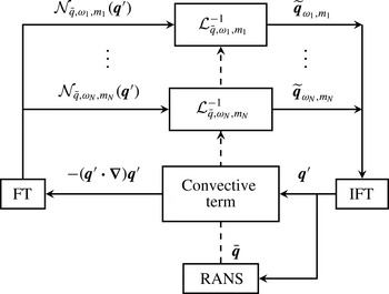
, as illustrated in figure 2.
Schematic representation of the full nonlinear system in the point of view of the response of the linearised operator to a nonlinear forcing; inspired by Moarref et al. (Reference Moarref, Jovanović, Tropp, Sharma and Mckeon2014). Here, ‘FT’ refers to the Fourier transform (2.1) and ‘IFT’ refers to the inverse Fourier transform; ‘RANS’ refers to the Reynolds-averaged Navier–Stokes equations.

In § 3, we consider a locally parallel framework for axisymmetric compressible shear flows. This formulation allows a further Fourier decomposition in the streamwise direction, and so the linearised model is there written as
 ${\mathcal{L}}_{\bar{\boldsymbol{q}},\unicode[STIX]{x1D6FC},\unicode[STIX]{x1D714},m}$
, where
 $\unicode[STIX]{x1D6FC}$
is the axial wavenumber of the perturbation considered. This locally parallel flow assumption is then relaxed in the PSE-4D-Var approach of § 4.
Of interest in this paper is the characterisation of the operator
 ${\mathcal{L}}_{\bar{\boldsymbol{q}},\unicode[STIX]{x1D714},m}$
in terms of its response to an external forcing,
 $\unicode[STIX]{x1D63D}\widetilde{\boldsymbol{f}}_{\unicode[STIX]{x1D714},m}$
, which plays the role of the nonlinearities
 ${\mathcal{N}}_{\bar{\boldsymbol{q}},\unicode[STIX]{x1D714},m}(\boldsymbol{q}^{\prime })$
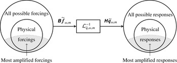
. As depicted in figure 3, we isolate the linearised operator for one frequency–wavenumber combination, and then characterise its response to forcing. For further consistency, an input matrix,
 $\unicode[STIX]{x1D63D}$
, is introduced, in order that the forcing be restricted to a subspace, spanned by the image of
 $\unicode[STIX]{x1D63D}$
. It can restrict, for instance, the forcing to act only on the momentum equation. Similarly, an output matrix,
 $\unicode[STIX]{x1D643}$
, is introduced to span an output observation space. It will be used explicitly in § 3.2 for the resolvent analysis and will be generalised to an observation operator in § 4.1 for taking data into account in the data-assimilation procedure.
Schematic representation of the study of the input/output behaviour of the linearised operator.

From a reduced-order-modelling perspective, as represented in figure 3, the goal is to shrink the space of all possible forcings to only those that will be highly amplified by the flow. Consideration of how the nonlinear term in the real jet exploits these mechanisms will be the subject of a later effort.
3 Locally parallel analysis
In this section, we present the mathematical formulation by which we explore the flow response to external harmonic forcing in a locally parallel setting. The critical-layer concept is first presented (§ 3.1) in order to highlight and discuss the associated physical mechanisms. We then use resolvent analysis to determine optimal forcing/response modes for base flows corresponding to several streamwise stations of the Mach 0.4 jet. The analysis highlights regions of the jet that are sensitive to external forcing; moreover, the optimal responses to forcing can be compared with measurements. The analysis gives a first indication of how linear wavepacket models might be enhanced with missing nonlinearities in order to match experimental data.
3.1 Critical layer
Critical layers arise in inviscid locally parallel shear flows as a singularity of the linearised Euler equations in wavenumber–frequency space, at points where the phase velocity,
 $c$
, is equal to the local fluid velocity (
 $c=\bar{U}(y_{c})$
). The position,
 $y_{c}$
, where this happens is called the critical point. This can be illustrated by considering the Rayleigh equation, here expressed in terms of the stream function,
 $\unicode[STIX]{x1D719}(x,y,t)=\widetilde{\unicode[STIX]{x1D719}}(y)\text{e}^{\text{i}\unicode[STIX]{x1D6FC}(x-ct)}$
,
 $$\begin{eqnarray}\displaystyle (\bar{U}(y)-c)\left(\frac{\unicode[STIX]{x2202}^{2}}{\unicode[STIX]{x2202}y^{2}}-\unicode[STIX]{x1D6FC}^{2}\right)\widetilde{\unicode[STIX]{x1D719}}-\frac{\unicode[STIX]{x2202}^{2}\bar{U}}{\unicode[STIX]{x2202}y^{2}}\widetilde{\unicode[STIX]{x1D719}}=0. & & \displaystyle\end{eqnarray}$$
At the critical point,
 $(\bar{U}(y_{c})-c)$
vanishes, and the highest derivative of the differential equation has a coefficient equal to zero, resulting in the said singularity. Solutions of this problem can be obtained by application of a Frobenius expansion (Adam Reference Adam1984; Maslowe Reference Maslowe1986; Campos, Oliveira & Kobayashi Reference Campos, Oliveira and Kobayashi1999; Brambley, Darau & Rienstra Reference Brambley, Darau and Rienstra2012) in the neighbourhood of the singularity, revealing a discontinuity (a phase jump of
 $\unicode[STIX]{x03C0}$
) of the stream function across the critical layer. These solutions comprise the continuous spectrum of the Rayleigh equation, with eigenvalues given by
 $c=U(y_{c})$
for some
 $y_{c}$
; we refer to these as critical-layer modes.
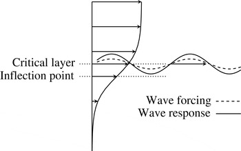
Having considered the homogeneous problem of (3.1), characteristic of intrinsic small disturbances in a shear flow, we consider the inhomogeneous problem, where background turbulence is understood as an extrinsic disturbance that forces the linear waves. Wave-like forces are considered, with the same phase speed and wavenumber as the linear wave, as illustrated in figure 4.
Schematic representation of a wave travelling over the mean flow and of a forcing having the same wave structure in the streamwise direction as the perturbation. The critical layer is the position where the phase velocity coincides with the local mean velocity.

Adjoint critical-layer modes can be determined (Drazin & Reid Reference Drazin and Reid2004) as
 $\widetilde{\unicode[STIX]{x1D719}}^{+}=\text{constant}\times \widetilde{\unicode[STIX]{x1D719}}/(\bar{U}(y)-c)$
. The adjoint modes become infinite at the critical point, and it can be shown that forcing at the critical point leads to infinite response. In a real flow, this singularity is regularised by other effects not present in the Rayleigh equation, such as viscosity (§ 3.2) or flow divergence (§ 4); both effects have low magnitude in the high-Reynolds-number turbulent jet considered here, and the critical layer is thus a region where high sensitivity to forcing can be expected. This high sensitivity has been explored in canonical shear flows in Tissot et al. (Reference Tissot, Zhang, Lajús, Cavalieri, Jordan and Colonius2015).
Alternatively, the singularity can be observed in the linear operator of the system expressed in primitive variables, by considering its response to an external force. In principle, a linear operator may lead to large responses in two ways (Schmid & Henningson Reference Schmid and Henningson2001). The first involves forcing the system at its resonance, which would be equivalent to exciting a shear flow with a frequency–wavenumber combination close to a solution of the dispersion relation, such as wavenumbers and frequencies corresponding to the K–H mode in mixing layers or jets. In the second case, even for an off-resonance excitation, the linear operator has a set of non-orthogonal eigenfunctions that, when considered in combination, can also produce a large response. These possibilities of large response have been discussed by McKeon & Sharma (Reference Mckeon and Sharma2010) in the case of turbulent pipe flows, where the role of critical layers was emphasised. Here, we discuss their observations by considering a 2D Cartesian
 $(x,y)$
incompressible viscous and parallel flow, forced via the momentum equations, where the use of normal modes allows the equations to be recast in matrix form as
 $$\begin{eqnarray}\displaystyle \left(\begin{array}{@{}c@{}}\tilde{u} \\ \tilde{v}\\ \tilde{p}\end{array}\right)=\left(\begin{array}{@{}ccc@{}}\text{i}\unicode[STIX]{x1D6FC}(\bar{U}-c)-\displaystyle \frac{1}{Re}\unicode[STIX]{x1D6FB}^{2} & \displaystyle \frac{\unicode[STIX]{x2202}\bar{U}}{\unicode[STIX]{x2202}y} & \text{i}\unicode[STIX]{x1D6FC}\\ 0 & \text{i}\unicode[STIX]{x1D6FC}(\bar{U}-c)-\displaystyle \frac{1}{Re}\unicode[STIX]{x1D6FB}^{2} & \displaystyle \frac{\unicode[STIX]{x2202}\cdot }{\unicode[STIX]{x2202}y}\\ \text{i}\unicode[STIX]{x1D6FC} & \displaystyle \frac{\unicode[STIX]{x2202}\cdot }{\unicode[STIX]{x2202}y} & 0\end{array}\right)^{-1}\left(\begin{array}{@{}c@{}}\tilde{f}_{x}\\ \tilde{f}_{y}\\ 0\end{array}\right), & & \displaystyle\end{eqnarray}$$
where
 $\unicode[STIX]{x1D6FB}^{2}=-\unicode[STIX]{x1D6FC}^{2}+\unicode[STIX]{x2202}^{2}/\unicode[STIX]{x2202}y^{2}$
. For high Reynolds number,
 $Re$
, the linear operator becomes ill-conditioned at the critical layer, as the convective terms composing the main diagonal tend to zero. This situation corresponds to a resonance of a critical-layer mode. Additionally, the presence of
 $\unicode[STIX]{x2202}U/\unicode[STIX]{x2202}y$
in an off-diagonal term clearly highlights that the operator is not self-adjoint. A strong shear, coupling the velocity components, is a source of non-normality which may intensify the forcing response independently of the critical-layer effect. In the following section, we compute optimal forcing and responses of the forced problem discussed above in the case of a turbulent compressible axisymmetric jet flow.
3.2 Resolvent analysis
Resolvent analysis provides orthogonal modes for both forcing and response, these being ranked according to the gain. The method is first presented in § 3.2.1. In § 3.2.2, it is applied to experimentally measured axisymmetric jet profiles.
3.2.1 Formulation
Let the output response,
 $\unicode[STIX]{x1D643}\widetilde{\boldsymbol{q}}_{\unicode[STIX]{x1D6FC},\unicode[STIX]{x1D714},m}$
, where
 $\unicode[STIX]{x1D643}$
is an observation operator, be rewritten in terms of the forcing as follows:
 $$\begin{eqnarray}\displaystyle \unicode[STIX]{x1D643}\widetilde{\boldsymbol{q}}_{\unicode[STIX]{x1D6FC},\unicode[STIX]{x1D714},m}=\unicode[STIX]{x1D643}{\mathcal{L}}_{\bar{\boldsymbol{q}},\unicode[STIX]{x1D6FC},\unicode[STIX]{x1D714},m}^{-1}\unicode[STIX]{x1D63D}\widetilde{\boldsymbol{f}}_{\bar{\boldsymbol{q}},\unicode[STIX]{x1D6FC},\unicode[STIX]{x1D714},m}=R_{\bar{\boldsymbol{q}},\unicode[STIX]{x1D6FC},\unicode[STIX]{x1D714},m}\widetilde{\boldsymbol{f}}_{\bar{\boldsymbol{q}},\unicode[STIX]{x1D6FC},\unicode[STIX]{x1D714},m}, & & \displaystyle\end{eqnarray}$$
where
 $R_{\bar{\boldsymbol{q}},\unicode[STIX]{x1D6FC},\unicode[STIX]{x1D714},m}=\unicode[STIX]{x1D643}{\mathcal{L}}_{\bar{\boldsymbol{q}},\unicode[STIX]{x1D6FC},\unicode[STIX]{x1D714},m}^{-1}\unicode[STIX]{x1D63D}$
is the resolvent operator (Schmid Reference Schmid2007). Once the problem is discretised, the operators become matrices, and will be considered as such in what follows. The goal of the analysis is to determine the forcing such that the norm of the associated response is maximised,
 $$\begin{eqnarray}\displaystyle \max _{\widetilde{\boldsymbol{f}}_{\unicode[STIX]{x1D6FC},\unicode[STIX]{x1D714},m}}\frac{\Vert \unicode[STIX]{x1D643}\widetilde{\boldsymbol{q}}_{\unicode[STIX]{x1D6FC},\unicode[STIX]{x1D714},m}\Vert _{\unicode[STIX]{x1D652}}^{2}}{\Vert \widetilde{\boldsymbol{f}}_{\unicode[STIX]{x1D6FC},\unicode[STIX]{x1D714},m}\Vert _{\unicode[STIX]{x1D652}}^{2}}=\frac{\Vert R_{\bar{\boldsymbol{q}},\unicode[STIX]{x1D6FC},\unicode[STIX]{x1D714},m}\widetilde{\boldsymbol{f}}_{\unicode[STIX]{x1D6FC},\unicode[STIX]{x1D714},m}\Vert _{\unicode[STIX]{x1D652}}^{2}}{\Vert \widetilde{\boldsymbol{f}}_{\unicode[STIX]{x1D6FC},\unicode[STIX]{x1D714},m}\Vert _{\unicode[STIX]{x1D652}}^{2}}, & & \displaystyle\end{eqnarray}$$
where
 $\ast$
applied to matrices implies conjugate transpose, the weighted norm,
 $\Vert \cdot \Vert _{\unicode[STIX]{x1D652}}$
, is associated with the inner product,
 $(\cdot ,\unicode[STIX]{x1D652}\cdot )$
, with
 $\unicode[STIX]{x1D652}$
a definite positive Hermitian matrix,
 $(\cdot \,,\cdot )$
the Euclidean inner product and
 $\Vert \cdot \Vert$
the Euclidean norm. For simplicity, it is considered that the weighted norm is the same in the input and output spaces. The maximisation of the Rayleigh quotient (3.4) can be achieved by means of the following singular value decomposition:
 $$\begin{eqnarray}\displaystyle (\unicode[STIX]{x1D652}^{1/2})^{\ast }R_{\bar{\boldsymbol{q}},\unicode[STIX]{x1D6FC},\unicode[STIX]{x1D714},m}(\unicode[STIX]{x1D652}^{-1/2})^{\ast }=\unicode[STIX]{x1D650}\unicode[STIX]{x1D72E}\unicode[STIX]{x1D651}^{\ast }, & & \displaystyle\end{eqnarray}$$
where
 $\unicode[STIX]{x1D652}^{1/2}$
is defined by the Cholesky decomposition,
 $\unicode[STIX]{x1D652}=\unicode[STIX]{x1D652}^{1/2}(\unicode[STIX]{x1D652}^{1/2})^{\ast }$
,
 $\unicode[STIX]{x1D650}=(\unicode[STIX]{x1D650}_{1},\ldots ,\unicode[STIX]{x1D650}_{N})$
and
 $\unicode[STIX]{x1D651}=(\unicode[STIX]{x1D651}_{1},\ldots ,\unicode[STIX]{x1D651}_{N})$
are orthonormal matrices and
 $\unicode[STIX]{x1D72E}$
is a diagonal matrix. We define the optimal forcing modes (OF) as
 $\unicode[STIX]{x1D731}_{i}=(\unicode[STIX]{x1D652}^{-1/2})^{\ast }\unicode[STIX]{x1D651}_{i}$
and the associated optimal response modes (OR) as
 $\unicode[STIX]{x1D733}_{i}=(\unicode[STIX]{x1D652}^{-1/2})^{\ast }\unicode[STIX]{x1D650}_{i}$
. The Hankel singular values,
 $\unicode[STIX]{x1D70E}_{i}$
, diagonal elements of
 $\unicode[STIX]{x1D72E}$
sorted in descending order, indicate the gains associated with forcing–response mode pairs. Indeed, we obtain the relationship
 $$\begin{eqnarray}\displaystyle \unicode[STIX]{x1D643}{\mathcal{L}}_{\bar{\boldsymbol{q}},\unicode[STIX]{x1D6FC},\unicode[STIX]{x1D714},m}^{-1}\unicode[STIX]{x1D63D}\unicode[STIX]{x1D731}_{i}=\unicode[STIX]{x1D70E}_{i}\unicode[STIX]{x1D733}_{i}, & & \displaystyle\end{eqnarray}$$
which shows that the optimal response is that of the optimal forcing amplified by the corresponding Hankel singular value
 $\unicode[STIX]{x1D70E}_{i}$
.
3.2.2 Resolvent analysis in an axisymmetric compressible jet
Resolvent analysis is applied in a locally parallel jet configuration and results are compared with measurements. As discussed previously, linear wavepackets computed using the homogeneous linearised system closely match measurements performed in an
 $M=0.4$
jet up to the end of the potential core, downstream of which the agreement deteriorates. We use resolvent analysis to explore whether this discrepancy might be remedied by considering optimally forced wavepackets.
In performing the resolvent analysis, we assume the jet flow to be viscous, compressible, isothermal and axisymmetric in a locally parallel setting. The base flows are taken from the measurements of Cavalieri et al. (Reference Cavalieri, Rodriguez, Jordan, Colonius and Gervais2013). In order to numerically converge the resolvent analysis, a lower Reynolds number than that of the experiment must be used (Meseguer & Trefethen Reference Meseguer and Trefethen2003); this is chosen as
 $Re=10\,000$
. As discussed in § 3.1, this viscosity regularises the solution, avoiding infinite responses. Due to the locally parallel flow assumption, only the axial component of the base-flow velocity is used, and the thermodynamic variables are determined using the Crocco–Busemann relation and the perfect gas law, thus defining the base flow as
 $\bar{\boldsymbol{q}}=(\bar{U},0,\bar{T},\bar{\unicode[STIX]{x1D70C}})^{\text{T}}$
. The viscosity
 $\bar{\unicode[STIX]{x1D707}}$
is determined using Sutherland’s law. The bulk viscosity is taken as
 $\unicode[STIX]{x1D707}_{B}=0.6\unicode[STIX]{x1D707}$
for air in accordance with Freund (Reference Freund1997). The equations are supplemented with homogeneous Dirichlet boundary conditions in the far field, as done in several previous studies (Hanifi, Schmid & Henningson Reference Hanifi, Schmid and Henningson1996; Gloor, Obrist & Kleiser Reference Gloor, Obrist and Kleiser2013). Application of a non-reflecting boundary condition is more accurate, using asymptotic (Gudmundsson Reference Gudmundsson2010) or characteristic methods (Poinsot & Lele Reference Poinsot and Lele1992). Nonetheless, the exponentially decaying modes in a sufficiently large computation domain will generate only negligible reflected waves. The full set of equations in cylindrical coordinates under such assumptions is provided in appendix A.
The equations are discretised and solved on a Chebyshev grid using a spectral collocation method (Weideman & Reddy Reference Weideman and Reddy2000) in the radial direction. To compute the singular value decomposition of the resolvent operator, one must define the matrices
 $\unicode[STIX]{x1D63D}$
and
 $\unicode[STIX]{x1D643}$
, and the norm
 $\Vert \cdot \Vert _{\unicode[STIX]{x1D652}}$
. We make the choice of restricting the input–output spaces to clarify physical interpretation of the results. Given the relatively low Mach number, nonlinearities of the continuity equation can be neglected (see the low-Mach-number limit in Alazard Reference Alazard2006). Moreover, since we are studying a cold jet, we can also neglect the nonlinear terms arising in the energy equation, such as the transport of the fluctuating temperature by the velocity fluctuations. We thus constrain the nonlinearities to act solely on the momentum equation. Moreover, in order to simplify interpretation, we focus on outputs in the momentum equations also, which leads to the matrices
 $$\begin{eqnarray}\displaystyle \unicode[STIX]{x1D63D}=\left(\begin{array}{@{}cc@{}}1 & 0\\ 0 & 1\\ 0 & 0\\ 0 & 0\end{array}\right),\quad \unicode[STIX]{x1D643}=\left(\begin{array}{@{}cccc@{}}1 & 0 & 0 & 0\\ 0 & 1 & 0 & 0\end{array}\right). & & \displaystyle\end{eqnarray}$$
Numerical tests show that the results remain qualitatively the same if the output matrix
 $\unicode[STIX]{x1D643}$
is the identity matrix. We recall that, despite the simplifications in the input/output behaviour, the full linearised equations for compressible flow are used.
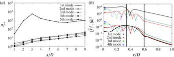
Characterisation of the optimal forcing–response modes. (a) Optimal response energy gain
 $\unicode[STIX]{x1D70E}_{i}^{2}$
for all axial positions for
 $St=0.6$
. (b) Optimal forcing/response at
 $x/D=8$
. For clarity, the forcing modes
 $\unicode[STIX]{x1D731}_{i}$
, in solid lines, have been multiplied by
 $10^{-3}$
. The associated responses
 $\unicode[STIX]{x1D70E}_{i}\unicode[STIX]{x1D733}_{i}$
are in dashed lines. Vertical solid: critical layer, vertical dashed: inflection point.

For compressible flows, as discussed in Hanifi et al. (Reference Hanifi, Schmid and Henningson1996) and Rowley, Colonius & Murray (Reference Rowley, Colonius and Murray2004), there exists no unique choice for the norm definition. Since we have restricted the inputs and outputs to the momentum equations, these norms simplify to the standard incompressible energy norm;
 $\unicode[STIX]{x1D652}$
is then defined such that
 $\Vert \unicode[STIX]{x1D643}\widetilde{\boldsymbol{q}}\Vert _{\unicode[STIX]{x1D652}}^{2}=\int _{\unicode[STIX]{x1D6FA}}(\bar{\unicode[STIX]{x1D70C}}/2)(\widetilde{u}^{\ast }\widetilde{u}+\widetilde{v}^{\ast }\widetilde{v})r\,\text{d}r$
.
In what follows, the phase velocity,
 $c$
, is that predicted by a PSE computation for the same jet, detailed in § 4.1.1. We have taken a real-valued
 $c$
, obtained as
 $\unicode[STIX]{x1D714}/\text{Re}(\unicode[STIX]{x1D6FC})$
,
 $\unicode[STIX]{x1D6FC}$
being the local wavenumber in the PSE computation. The justification of this choice is given in appendix B. The axisymmetric mode,
 $m=0$
, is considered, as it is the most acoustically efficient (Cavalieri et al.
Reference Cavalieri, Jordan, Colonius and Gervais2012, Reference Cavalieri, Rodriguez, Jordan, Colonius and Gervais2013), and
 $St=0.6$
is arbitrarily chosen to illustrate the salient features of forced-wavepacket behaviour.
The resolvent analysis identifies a basis of forcing modes spanning
 $\text{Ker}(\unicode[STIX]{x1D643}{\mathcal{L}}_{\bar{\boldsymbol{q}},\unicode[STIX]{x1D6FC},\unicode[STIX]{x1D714},m}^{-1}\unicode[STIX]{x1D63D})^{\text{T}}$
and a basis of response modes spanning
 $\text{Im}(\unicode[STIX]{x1D643}{\mathcal{L}}_{\bar{\boldsymbol{q}},\unicode[STIX]{x1D6FC},\unicode[STIX]{x1D714},m}^{-1}\unicode[STIX]{x1D63D})$
. Figure 5(a) shows the optimal energy gain
 $\unicode[STIX]{x1D70E}_{i}^{2}$
of the five first modes as a function of axial position. This figure shows that for all axial positions, the first optimal forcing–response mode pair clearly dominates. This suggests that the optimal forcing–response mode pair is the most relevant for the dynamics of wavepackets forced by background turbulence. This idea is supported by the recent work of Beneddine et al. (Reference Beneddine, Sipp, Arnault, Dandois and Lesshafft2016), which shows that when the first optimal energy gain is clearly higher than the others and if the turbulent forcing does not project preferentially onto a suboptimal mode, the response is dominated by the first optimal response mode. Figure 5(b) shows the radial structure of the first four optimal forcing modes at
 $x/D=8$
and of the associated responses. Beyond the fact that the first optimal response mode dominates by one order of magnitude, the shape of the forcing and the associated response are typical of the critical-layer mechanism highlighted in the direct forcing study in Tissot et al. (Reference Tissot, Zhang, Lajús, Cavalieri, Jordan and Colonius2015). While the forcing has broad radial support, its maximum is at the critical layer and the response has here one dip and a phase jump of approximately
 $\unicode[STIX]{x03C0}$
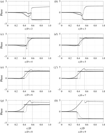
(phases are shown in appendix C, figure 22), consistent with the shape of critical-layer modes, and indicative of a vortex-like structure, where axial velocity fluctuations at either side of the vortex are in phase opposition, and zero amplitude is found at the vortex centre (see the discussion in Cavalieri et al.
Reference Cavalieri, Rodriguez, Jordan, Colonius and Gervais2013). The higher modes show several dips and can be interpreted as functions that span the response to less relevant turbulent structures. The dominance of the first mode pair is encouraging vis-à-vis an eventual reduced-order model, and so in what follows we consider only this first mode pair.
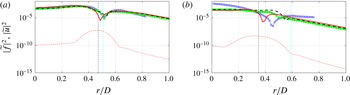
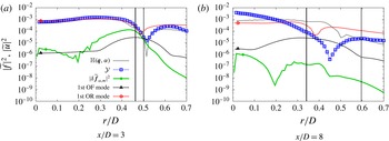
Comparison of optimal forcing modes (red dashed lines) and optimal response modes (red solid lines) of axial velocity fluctuation at
 $x/D=3$
(a) and
 $x/D=8$
(b) with experimental data (blue squares) and the solution of the homogeneous linear problem (LEE, green line with solid dots; PSE, black dashed line). Here,
 $St=0.6$
,
 $Re=10\,000$
,
 $M=0.4$
. The phase velocity
 $c$
predicted by the PSE is used. The vertical dashed line is the critical-layer position and the vertical dash-dotted line is the inflectional point position.

In figure 6, we show the power spectral density (PSD) of the axial perturbation velocity obtained by the resolvent analysis compared with time-resolved particle image velocimetry (PIV) measurements (TRPIV), and also with two linear wavepacket models, solutions of either the linearised Euler equations (LEE) or the PSE. The LEE solutions are taken from Zhang et al. (Reference Zhang, Jordan, Lehnasch, Cavalieri and Agarwal2014). We focus the comparison on two emblematic positions:
 $x/D=3$
, which typifies results upstream of the end of the potential core, where the homogeneous linear framework matches the data closely, and
 $x/D=8$
, typifying results obtained downstream of the potential core, where linear theory fails. Results for other axial stations are shown in appendix C, figure 21.
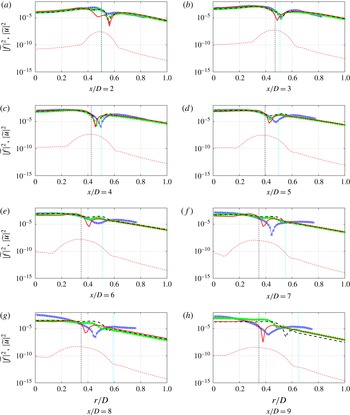
In the experimental results, upstream of
 $x/D\sim 5$
, the first proper orthogonal decomposition (POD) mode of the TRPIV data for
 $m=0$
shows that the turbulent jet flow comprises a vortex-like signature in this region (Cavalieri et al.
Reference Cavalieri, Rodriguez, Jordan, Colonius and Gervais2013). We can also see that, in this region, the linear wavepacket models (PSE and LEE) correctly capture this structure, as these curves collapse with the TRPIV data. This indicates that the homogeneous linear wavepacket model is able to predict the behaviour of the K–H instability in the upstream part of the jet, which undergoes exponential growth in
 $x$
. The resolvent optimal response modes, although corresponding to a forced-wavepacket scenario, clearly dynamically different from the homogeneous linear wavepackets, also match the measurement upstream of
 $x/D\sim 5$
. The similarities between the results of the homogeneous and the forced problems suggest that in the upstream region resolvent analysis leads to a most amplified response corresponding to a pseudo-resonance of the Kelvin–Helmholtz mode; the flow response is approximately the same for both upstream excitation (in the homogeneous problem) and forcing by nonlinearities (in the forced problem).
Downstream of the end of the potential core, on the other hand, the homogeneous linear models (PSE or LEE) predict a quite different radial structure, as can be seen at
 $x/D=8$
, figure 6, or in figure 21. The measurement shows that the flow field in these regions retains a vortex-like structure possessing a local dip in amplitude at approximately
 $r/D\sim 0.4$
(this dip in amplitude is a signature of phase opposition of disturbances on either side of the lipline, as previously discussed) which is not captured by the linear homogeneous wavepacket model. When forcing by nonlinearities is considered in the resolvent analysis, the optimal response displays a radial structure similar to that of the experimentally educed wavepacket. This is an encouraging indication that the notion of forced linear wavepackets may correspond to what is happening in the flow downstream of the potential core.
We note here that the position of the dip does not always correspond exactly with experimental results. This position is sensitive to the perturbation phase velocity
 $c$
, which fixes the critical-layer position. The forced wavepacket, which we assume to be present in experiments, may have a slightly different phase velocity from the unforced wavepacket, explaining the observed discrepancies. Indeed, as shown in appendix B, the agreement at
 $x/D=8$
can be slightly improved with a modification of
 $c$
. Selection of
 $c$
from linear PSE results remains preferable, as this is a choice based on first principles and not a posteriori.
The comparison can be extended to other Strouhal numbers and axial stations by means of an agreement metric between any pair taken from TRPIV, PSE and OR; we thus define the metric
 $\unicode[STIX]{x1D6FD}$
(shown here between PSE and TRPIV, for example),
 $$\begin{eqnarray}\displaystyle \unicode[STIX]{x1D6FD}_{PSE-TRPIV}(x,St)=\frac{(\unicode[STIX]{x1D643}\widetilde{\boldsymbol{q}}_{PSE},{\mathcal{Y}})_{r}}{\sqrt{(\unicode[STIX]{x1D643}\widetilde{\boldsymbol{q}}_{PSE},\unicode[STIX]{x1D643}\widetilde{\boldsymbol{q}}_{PSE})_{r}({\mathcal{Y}},{\mathcal{Y}})_{r}}}, & & \displaystyle\end{eqnarray}$$
where the
 ${\mathcal{Y}}$
are the PSD of velocity components from experimental measurements and
 $$\begin{eqnarray}\displaystyle (\boldsymbol{a},\boldsymbol{b})_{r}=\int _{r_{b}}^{r_{t}}a^{\ast }(r)b(r)r\,\text{d}r, & & \displaystyle\end{eqnarray}$$
 $r_{b}$
and
 $r_{t}$
defining the integration range for each variable. For the axisymmetric mode considered, only
 $\widetilde{u}$
and
 $\widetilde{v}$
are involved in the calculation, since these are the quantities available from the experimental results. The results for the absolute values of
 $\unicode[STIX]{x1D6FD}$
(
 $|\unicode[STIX]{x1D6FD}|$
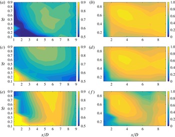
) between TRPIV and PSE or OR are shown in figure 7. When two quantities have similar radial structure, the value of
 $|\unicode[STIX]{x1D6FD}|$
is close to unity.
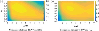
In figure 7(a), we see that PSE matches the experimental data well upstream of the end of the potential core, especially for
 $St=0.3{-}0.9$
, and the agreement deteriorates in the downstream region. This result has been noted in Cavalieri et al. (Reference Cavalieri, Rodriguez, Jordan, Colonius and Gervais2013), for example. For the comparison between TRPIV and OR, we see in figure 7(b) that the values of the
 $\unicode[STIX]{x1D6FD}$
metric are globally higher than those obtained for TRPIV and PSE. Moreover,
 $|\unicode[STIX]{x1D6FD}|$
does not decay in the downstream region as significantly as in figure 7(a). This result has already been inferred and discussed from figure 6 above, but figure 7 is a useful means by which to compress the comparisons for all frequencies and axial positions into a single figure.
Values of
 $|\unicode[STIX]{x1D6FD}|$
. Here,
 $c$
is determined from the PSE calculation.

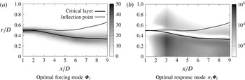
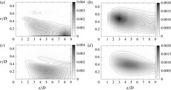
Figure 8(a) shows a map of the optimal forcing mode
 $\unicode[STIX]{x1D731}_{1}$
, whose norm is fixed to 1. With this arbitrary normalisation we cannot evaluate the downstream evolution of forced wavepackets; the purpose of the plot is to examine the radial structure of optimal forcing and response for different axial stations. It is clear that for all
 $x/D$
the optimal forcing is concentrated around the critical layer. The associated response,
 $\unicode[STIX]{x1D70E}_{1}\unicode[STIX]{x1D733}_{1}$
, is shown in figure 8(b). The response also follows the critical layer, with a dip in amplitude consistently close to the critical-layer position, and a clear signature of a vortex-like structure. A maximum response appears at
 $x/D=3$
, in keeping with the peak at that position of the optimal energy gain in figure 5(a).
The PSD of the first optimal forcing and response modes along the axial direction at
 $St=0.6$
, with
 $c$
determined by PSE. The solid line is the critical-layer position and the dashed line is the inflection point position.

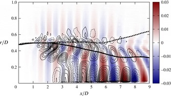
Finally, spatial reconstructions of the optimal forcings and responses (figure 9) at
 $x/D=3$
and
 $x/D=8$
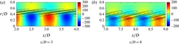
show that the optimal forcing is inclined against the shear, suggesting an exploitation of non-normality by the Orr mechanism.
Spatial reconstruction of the streamwise component of the optimal response (colour) and of the optimal forcing (isolines, solid for positive, dashed for negative).

To summarise, the first optimal forcing mode dominates the higher-order ones and shows a maximum at the critical layer for all axial positions. The response is consistent with the observed flow behaviour downstream of the end of the potential core, supporting the idea that a forced-wavepacket model may be what is needed to describe features present in this region of the jet. Finally, a spot of high sensitivity to forcing is found at
 $x/D=3$
for
 $St=0.6$
, which is where the K–H mode becomes neutral and thus close, in the complex plane, to the real wavenumber associated with the forcing. Because of the locally parallel assumption of the resolvent analysis, conclusions about relationships between different axial positions can be difficult to draw. In § 4.1, we therefore complement the study with a non-parallel approach, PSE-4D-Var, which accommodates the true structure of the mean flow and permits a more complete consideration of the spatially convective nature of the flow.
4 Non-parallel analysis
In this section, we drop the parallel-flow assumption, used in the previous section, and consider a slowly diverging base flow, taken from the mean velocity profile of the same Mach 0.4 jet, using the parabolised stability equations. Having explored the local dynamics with locally parallel resolvent analysis, PSE allows us to take into account the complete wavepacket structure starting from the Kelvin–Helmholtz instability near the nozzle exit. The local wavenumber in the PSE framework nonetheless permits connection with the locally parallel analysis.
Based on PSE, we explore the missing pieces of the linear model using a data-driven approach, 4D-Var. We use a specific variant of this, called weak-constraint variational data assimilation (Papadakis Reference Papadakis2007). This estimation problem is formulated as an optimisation problem, where we authorise modifications of the initial conditions and of an external forcing in the PSE, considered as modelling uncertainties. As discussed in § 2, the external forcing can be interpreted as a nonlinear term, not taken into account by the linear model, and which we would like to identify. We are thus searching, via an inverse problem, for the minimum forcing, interpreted as the effect of nonlinearities, necessary to produce linear waves that match measurements. In what follows, we use 4D-Var to solve three data-assimilation problems. We first solve a standard sensitivity problem, analogous to the previous section, here extended to a diverging base flow. We then compute a 4D-Var sensitivity that corresponds to the sensitivity of PSE to forcing that would reduce the discrepancy between model and measurements. Finally, the entire minimisation problem is solved to convergence.
4.1 The PSE-4D-Var approach
4.1.1 Formulation
The PSE (Herbert Reference Herbert1997) allow instability wave evolution over a slowly varying base flow to be modelled. The formulation used here is similar to that used in previous works (Gudmundsson Reference Gudmundsson2010; Cavalieri et al.
Reference Cavalieri, Rodriguez, Jordan, Colonius and Gervais2013; Sasaki Reference Sasaki2015). The assumption of a slowly varying base flow allows (Crighton & Gaster Reference Crighton and Gaster1976) decomposition of the perturbation associated with mode
 $(\unicode[STIX]{x1D714},m)$
into slowly and rapidly varying (wave-like) parts (Herbert Reference Herbert1997),
 $$\begin{eqnarray}\displaystyle \widetilde{\boldsymbol{q}}_{\unicode[STIX]{x1D714},m}(x,r)=\boldsymbol{q}(x,r)\text{e}^{\text{i}\int _{0}^{x}\unicode[STIX]{x1D6FC}(\unicode[STIX]{x1D709})\,\text{d}\unicode[STIX]{x1D709}}. & & \displaystyle\end{eqnarray}$$
Here,
 $\boldsymbol{q}(x,r)$
is the slowly varying part and
 $\text{e}^{\text{i}\int _{0}^{x}\unicode[STIX]{x1D6FC}(\unicode[STIX]{x1D709})\,\text{d}\unicode[STIX]{x1D709}}$
is the wave-like part. The
 $(\unicode[STIX]{x1D714},m)$
index is dropped for compactness. The decomposition (4.1) is introduced into the compressible Navier–Stokes equations. The nonlinear terms are then neglected, assuming small perturbations, and the first axial derivatives of
 $\unicode[STIX]{x1D6FC}$
and second axial derivatives of
 $\boldsymbol{q}$
are neglected, assuming a slow variation of these variables in the streamwise direction. We thus obtain an equation of the form
 $$\begin{eqnarray}\displaystyle \unicode[STIX]{x1D640}\frac{\unicode[STIX]{x2202}\boldsymbol{q}}{\unicode[STIX]{x2202}x}+(\unicode[STIX]{x1D63C}+\unicode[STIX]{x1D6FC}\unicode[STIX]{x1D63E})\boldsymbol{q}=0, & & \displaystyle\end{eqnarray}$$
where the matrix
 $\unicode[STIX]{x1D63C}$
contains discrete radial derivatives. The domain,
 $x/D=[0,L]$
,
 $r/D=[0,\infty ]$
, is discretised using
 $N_{x}$
points in the axial direction and
 $N_{r}$
Chebyshev collocation points in the radial direction. Details of derivation of the PSE for compressible flow in cylindrical coordinates are given in Sasaki (Reference Sasaki2015).
The decomposition (4.1) is a priori not unique because of the presence of the
 $x$
variable in
 $\boldsymbol{q}(x,r)$
as well as in
 $\unicode[STIX]{x1D6FC}(x)$
, and because no evolution equation is given for
 $\unicode[STIX]{x1D6FC}$
. In order to overcome this ambiguity, a normalisation constraint is added (see Herbert Reference Herbert1997) such that the exponential dependence (real and imaginary) is absorbed by the wave-like term
 $\text{e}^{\text{i}\int _{0}^{x}\unicode[STIX]{x1D6FC}(\unicode[STIX]{x1D709})\,\text{d}\unicode[STIX]{x1D709}}$
:
 $$\begin{eqnarray}\displaystyle \left(\boldsymbol{q},\frac{\unicode[STIX]{x2202}\boldsymbol{q}}{\unicode[STIX]{x2202}x}\right)_{r}=\int _{0}^{\infty }\boldsymbol{q}\boldsymbol{\cdot }\frac{\unicode[STIX]{x2202}\boldsymbol{q}}{\unicode[STIX]{x2202}x}r\,\text{d}r=0. & & \displaystyle\end{eqnarray}$$
Starting with
 $(\boldsymbol{q}_{0},\unicode[STIX]{x1D6FC}_{0})$
, often taken as the K–H mode, solution of the locally parallel problem at the initial position,
 $\boldsymbol{q}(x,r)$
, can be obtained by integrating (4.2) in space using an implicit Euler scheme, with iterations in
 $\unicode[STIX]{x1D6FC}$
such that the constraint (4.3) is respected (Gudmundsson Reference Gudmundsson2010). The linear PSE procedure allows wavepackets for each frequency–azimuthal mode pair to be propagated independently.
In the 4D-Var under weak dynamical constraint, we would like the solution,
 $\boldsymbol{q}(x,r)$
, to follow the observations, and we consider that this solution respects the model – here the linear PSE – only in a weak sense. In order to relax this constraint, we introduce a forcing term,
 $\boldsymbol{f}$
, interpreted as the effect of nonlinearities, and an initial condition perturbation,
 $\boldsymbol{\unicode[STIX]{x1D702}}$
. Combining the nonlinear forcing with (4.2) and (4.3), the forced parabolised stability equations can be written as
 $$\begin{eqnarray}\displaystyle \left.\begin{array}{@{}c@{}}\displaystyle \unicode[STIX]{x1D640}\frac{\unicode[STIX]{x2202}\boldsymbol{q}}{\unicode[STIX]{x2202}x}+(\unicode[STIX]{x1D63C}+\unicode[STIX]{x1D6FC}\unicode[STIX]{x1D63E})\boldsymbol{q}=\boldsymbol{f},\\ \displaystyle \left(\boldsymbol{q},\frac{\unicode[STIX]{x2202}\boldsymbol{q}}{\unicode[STIX]{x2202}x}\right)_{r}=\boldsymbol{q}^{\ast }\unicode[STIX]{x1D652}_{r}\frac{\unicode[STIX]{x2202}\boldsymbol{q}}{\unicode[STIX]{x2202}x}=0,\\ \displaystyle \boldsymbol{q}(0,r)=\boldsymbol{q}_{0}+\boldsymbol{\unicode[STIX]{x1D702}},\quad \unicode[STIX]{x1D6FC}(0)=\unicode[STIX]{x1D6FC}_{0},\end{array}\right\} & & \displaystyle\end{eqnarray}$$
where
 $\unicode[STIX]{x1D652}_{r}$
is the discrete weight matrix associated with the inner product
 $(\cdot \,,\cdot )_{r}$
. It should be noted that we implicitly enforce the shape of the forcing as
 $$\begin{eqnarray}\displaystyle \widetilde{\boldsymbol{f}}_{\unicode[STIX]{x1D714},m}(x,r)=\boldsymbol{f}(x,r)\text{e}^{\text{i}\int _{0}^{x}\unicode[STIX]{x1D6FC}(\unicode[STIX]{x1D709})\,\text{d}\unicode[STIX]{x1D709}}, & & \displaystyle\end{eqnarray}$$
and we can define a forcing in physical space as
 $$\begin{eqnarray}\displaystyle \boldsymbol{f}_{\unicode[STIX]{x1D719}}(x,r,\unicode[STIX]{x1D703},t)=\frac{1}{(2\unicode[STIX]{x03C0})^{2}}\mathop{\sum }_{m}\int _{-\infty }^{\infty }\widetilde{\boldsymbol{f}}_{\unicode[STIX]{x1D714},m}(x,r)\text{e}^{\text{i}(m\unicode[STIX]{x1D703}-\unicode[STIX]{x1D714}t)}\,\text{d}\unicode[STIX]{x1D714}. & & \displaystyle\end{eqnarray}$$
This means that because a harmonic framework is used, the optimal forcing is constrained to have a wavepacket shape. This shape is indeed able to act efficiently on the instability wave because a forcing whose wavenumber matches that of the wavepacket should lead to the most significant dynamic effects. In principle,
 $\boldsymbol{f}$
could come, for instance, from a nonlinear PSE computation taking account of a reduced number of wave–wave interactions. In the present study, all possible nonlinear interactions are potentially considered via the inverse problem.
The objective of 4D-Var is to seek
 $(\boldsymbol{f},\boldsymbol{\unicode[STIX]{x1D702}})$
minimising
 $$\begin{eqnarray}\displaystyle {\mathcal{J}}(\boldsymbol{q},\unicode[STIX]{x1D6FC},\boldsymbol{f},\boldsymbol{\unicode[STIX]{x1D702}}) & = & \displaystyle \frac{1}{2}\int _{0}^{L}\Vert \mathbb{H}(\boldsymbol{q},\unicode[STIX]{x1D6FC})-{\mathcal{Y}}\Vert _{\unicode[STIX]{x1D652}_{o}}^{2}\,\text{d}x+\frac{1}{2}\Vert \mathbb{H}(\boldsymbol{q}_{L},\unicode[STIX]{x1D6FC}_{L})-{\mathcal{Y}}_{L}\Vert _{\unicode[STIX]{x1D652}_{T}}^{2}\nonumber\\ \displaystyle & & \displaystyle +\,\frac{1}{2}\int _{0}^{L}\Vert \boldsymbol{f}\Vert _{\unicode[STIX]{x1D652}_{f}}^{2}\,\text{d}x+\frac{1}{2}\Vert \boldsymbol{\unicode[STIX]{x1D702}}\Vert _{\unicode[STIX]{x1D652}_{\unicode[STIX]{x1D702}}}^{2},\end{eqnarray}$$
where
 $\mathbb{H}(\boldsymbol{q},\unicode[STIX]{x1D6FC})$
is an observation operator allowing passage from the state space to the observation space. The observation operator
 $\mathbb{H}(\boldsymbol{q},\unicode[STIX]{x1D6FC})$
is related to the output matrix
 $\unicode[STIX]{x1D643}$
, introduced in § 2, since both define the output space. Here, it is simply generalised to a nonlinear operator. The
 ${\mathcal{Y}}$
are associated observations, i.e. experimental measurements. A standard sensitivity problem is achieved choosing
 $$\begin{eqnarray}\displaystyle \mathbb{H}(\boldsymbol{q},\unicode[STIX]{x1D6FC})=\boldsymbol{q}\text{e}^{\text{i}\int _{0}^{x}\unicode[STIX]{x1D6FC}(\unicode[STIX]{x1D709})\,\text{d}\unicode[STIX]{x1D709}},\quad {\mathcal{Y}}=0. & & \displaystyle\end{eqnarray}$$
For the 4D-Var problem, we choose
 $$\begin{eqnarray}\displaystyle \mathbb{H}(\boldsymbol{q},\unicode[STIX]{x1D6FC})=\unicode[STIX]{x1D64C}|\boldsymbol{q}\text{e}^{\text{i}\int _{0}^{x}\unicode[STIX]{x1D6FC}(\unicode[STIX]{x1D709})\,\text{d}\unicode[STIX]{x1D709}}|^{2} & & \displaystyle\end{eqnarray}$$
and
 ${\mathcal{Y}}$
as the PSD of streamwise and radial velocity measurements. Here,
 $\unicode[STIX]{x1D64C}$
is a rectangular matrix of zeros and ones. Similarly to the output matrix
 $\unicode[STIX]{x1D643}$
in (3.7), rows of
 $\unicode[STIX]{x1D64C}$
contain a ‘one’ in order to select the components and the radial positions that are observed, here the axial and radial velocities for the positions where there are available TRPIV results. The terms
 $\boldsymbol{q}_{L}$
,
 $\unicode[STIX]{x1D6FC}_{L}$
and
 ${\mathcal{Y}}_{L}$
refer to the values of the variables or parameters at
 $x/D=L$
, where
 $L$
is the downstream end of the computational domain; we penalise errors in the terminal condition in order to avoid transient behaviour at the end of the domain of the adjoint equation, presented later.
The norms
 $\Vert \cdot \Vert _{\unicode[STIX]{x1D652}_{o}}$
,
 $\Vert \cdot \Vert _{\unicode[STIX]{x1D652}_{T}}$
,
 $\Vert \cdot \Vert _{\unicode[STIX]{x1D652}_{f}}$
and
 $\Vert \cdot \Vert _{\unicode[STIX]{x1D652}_{\unicode[STIX]{x1D702}}}$
are respectively associated with the inner products,
 $(\unicode[STIX]{x1D64C}^{\ast }\cdot ,\unicode[STIX]{x1D64C}^{\ast }\unicode[STIX]{x1D652}_{o}\cdot )_{r}$
,
 $(\unicode[STIX]{x1D64C}^{\ast }\cdot ,\unicode[STIX]{x1D64C}^{\ast }\unicode[STIX]{x1D652}_{T}\cdot )_{r}$
,
 $(\cdot ,\unicode[STIX]{x1D652}_{f}\cdot )_{r}$
and
 $(\cdot ,\unicode[STIX]{x1D652}_{\unicode[STIX]{x1D702}}\cdot )_{r}$
. The weight matrices,
 $\unicode[STIX]{x1D652}_{o}$
,
 $\unicode[STIX]{x1D652}_{T}$
,
 $\unicode[STIX]{x1D652}_{f}$
and
 $\unicode[STIX]{x1D652}_{\unicode[STIX]{x1D702}}$
, allow different degrees of confidence to be specified in the observations or in the PSE model. Finally, for later use, we define, for any
 $\unicode[STIX]{x1D648}\in \mathbb{R}^{N_{c}N_{r}\times N_{c}N_{r}}$
, the adjoint matrix
 $\unicode[STIX]{x1D648}^{+}=\unicode[STIX]{x1D652}_{r}^{-1}\unicode[STIX]{x1D648}^{\ast }\unicode[STIX]{x1D652}_{r}$
, such that
 $(\unicode[STIX]{x1D648}\boldsymbol{x},\boldsymbol{y})_{r}=(\boldsymbol{x},\unicode[STIX]{x1D648}^{+}\boldsymbol{y})_{r}$
.
4.1.2 Optimality system
The minimisation problem exposed in § 4.1.1 is a constrained optimisation problem. It consists in minimising (4.7) under the constraint (4.4). This problem is usually solved using a quasi-Newton algorithm, which requires the gradient of the cost functional,
 ${\mathcal{J}}$
, with respect to the control parameters,
 $(\boldsymbol{f},\boldsymbol{\unicode[STIX]{x1D702}})$
. Because the control parameter space is of large dimension, we use an adjoint method, where the gradient of the cost functional
 ${\mathcal{J}}$
, also called sensitivity, is determined by the integration of an adjoint equation (Gunzburger Reference Gunzburger2003). The direct and adjoint systems are then solved iteratively until convergence to the optimal solution.
The continuous adjoint PSE can be determined in different ways. The first consists in parabolising the adjoint LEE, as done by Dobrinsky (Reference Dobrinsky2002) for a receptivity problem. The second is to directly derive the adjoint PSE as in Pralits et al. (Reference Pralits, Airiau, Hanifi and Henningson2000) and Ansaldi & Airiau (Reference Ansaldi and Airiau2015) for a sensitivity analysis or as in Pralits, Hanifi & Henningson (Reference Pralits, Hanifi and Henningson2002) and Airiau et al. (Reference Airiau, Bottaro, Walther and Legendre2003) for flow control. For reasons of consistency between PSE and adjoint PSE, the latter method has been chosen.
In order to derive the adjoint equation, we introduce additional variables,
 $\unicode[STIX]{x1D740}$
,
 $\unicode[STIX]{x1D701}$
and
 $\unicode[STIX]{x1D743}$
, called Lagrange multipliers, whose role is to enforce the constraint (4.4). We then transform the constrained optimisation problem to an unconstrained one, defining the Lagrangian
 $$\begin{eqnarray}\displaystyle {\mathcal{L}}(\boldsymbol{q},\unicode[STIX]{x1D6FC},\boldsymbol{f},\boldsymbol{\unicode[STIX]{x1D702}},\unicode[STIX]{x1D740},\unicode[STIX]{x1D701},\unicode[STIX]{x1D743}) & = & \displaystyle {\mathcal{J}}(\boldsymbol{q},\unicode[STIX]{x1D6FC},\boldsymbol{f},\boldsymbol{\unicode[STIX]{x1D702}})\end{eqnarray}$$
 $$\begin{eqnarray}\displaystyle & & \displaystyle -\,\text{Re}\left(\int _{0}^{L}\left(\unicode[STIX]{x1D640}\frac{\unicode[STIX]{x2202}\boldsymbol{q}}{\unicode[STIX]{x2202}x}+(\unicode[STIX]{x1D63C}+\unicode[STIX]{x1D6FC}\unicode[STIX]{x1D63E})\boldsymbol{q}-\boldsymbol{f},\unicode[STIX]{x1D740}\right)_{r}\,\text{d}x\right)\end{eqnarray}$$
 $$\begin{eqnarray}\displaystyle & & \displaystyle -\,\text{Re}\left(\int _{0}^{L}\left(\boldsymbol{q},\frac{\unicode[STIX]{x2202}\boldsymbol{q}}{\unicode[STIX]{x2202}x}\right)_{r}\unicode[STIX]{x1D701}\,\text{d}x\right).\end{eqnarray}$$
 $$\begin{eqnarray}\displaystyle & & \displaystyle -\,\text{Re}((\boldsymbol{q}(0,r)-\boldsymbol{q}_{0}-\boldsymbol{\unicode[STIX]{x1D702}},\unicode[STIX]{x1D743})_{r}).\end{eqnarray}$$
Direct system:
 $$\begin{eqnarray}\displaystyle \left.\begin{array}{@{}c@{}}\displaystyle \unicode[STIX]{x1D640}\frac{\unicode[STIX]{x2202}\boldsymbol{q}}{\unicode[STIX]{x2202}x}+(\unicode[STIX]{x1D63C}+\unicode[STIX]{x1D6FC}\unicode[STIX]{x1D63E})\boldsymbol{q}=\boldsymbol{f},\\ \displaystyle \left(\boldsymbol{q},\frac{\unicode[STIX]{x2202}\boldsymbol{q}}{\unicode[STIX]{x2202}x}\right)_{r}=0\\ \displaystyle \boldsymbol{q}(0,r)=\boldsymbol{q}_{0}+\boldsymbol{\unicode[STIX]{x1D702}},\quad \unicode[STIX]{x1D6FC}(0)=\unicode[STIX]{x1D6FC}_{0}.\end{array}\right\} & & \displaystyle\end{eqnarray}$$
Adjoint system:
 $$\begin{eqnarray}\displaystyle \left.\begin{array}{@{}c@{}}\displaystyle -\unicode[STIX]{x1D640}^{+}\frac{\unicode[STIX]{x2202}\unicode[STIX]{x1D740}}{\unicode[STIX]{x2202}x}+\left(\unicode[STIX]{x1D63C}+\unicode[STIX]{x1D6FC}\unicode[STIX]{x1D63E}-\frac{\unicode[STIX]{x2202}\unicode[STIX]{x1D640}}{\unicode[STIX]{x2202}x}\right)^{+}\unicode[STIX]{x1D740}+\frac{\unicode[STIX]{x2202}\boldsymbol{q}}{\unicode[STIX]{x2202}x}(\unicode[STIX]{x1D701}-\unicode[STIX]{x1D701}^{\ast })-\boldsymbol{q}\frac{\unicode[STIX]{x2202}\unicode[STIX]{x1D701}^{\ast }}{\unicode[STIX]{x2202}x}=RHS_{1},\\ \displaystyle (\unicode[STIX]{x1D63E}\boldsymbol{q},\unicode[STIX]{x1D740})_{r}=RHS_{2},\\ \displaystyle \unicode[STIX]{x1D640}^{+}\unicode[STIX]{x1D740}(L,r)=RHS_{3},\\ \displaystyle \unicode[STIX]{x1D701}(L)=0.\end{array}\right\} & & \displaystyle\end{eqnarray}$$
The terms
 $RHS_{1}$
,
 $RHS_{2}$
and
 $RHS_{3}$
are expressed in appendix D and depend on the definition of the cost functional (4.7), especially on the observation operator.
Optimality condition:
 $$\begin{eqnarray}\displaystyle \left.\begin{array}{@{}c@{}}\displaystyle \frac{\unicode[STIX]{x2202}J}{\unicode[STIX]{x2202}\boldsymbol{f}}=\unicode[STIX]{x1D740}(x,r)+\unicode[STIX]{x1D652}_{f}\boldsymbol{f},\\ \displaystyle \frac{\unicode[STIX]{x2202}J}{\unicode[STIX]{x2202}\boldsymbol{\unicode[STIX]{x1D702}}}=\unicode[STIX]{x1D640}^{+}\unicode[STIX]{x1D740}(0,r)+\boldsymbol{q}_{0}\unicode[STIX]{x1D701}^{\ast }(0)+\unicode[STIX]{x1D652}_{\unicode[STIX]{x1D702}}\boldsymbol{\unicode[STIX]{x1D702}}.\end{array}\right\} & & \displaystyle\end{eqnarray}$$
The minimisation problem can be solved iteratively (Bewley, Moin & Temam Reference Bewley, Moin and Temam2001) in a computationally efficient manner using this optimality system. Once the direct system (4.11) is solved,
 $(\boldsymbol{q},\unicode[STIX]{x1D6FC})$
are known and one can integrate the adjoint system (4.12) backwards in space to obtain
 $(\unicode[STIX]{x1D740},\unicode[STIX]{x1D701},\unicode[STIX]{x1D743})$
, and finally obtain the gradients
 $(\unicode[STIX]{x2202}J/\unicode[STIX]{x2202}\boldsymbol{f},\unicode[STIX]{x2202}J/\unicode[STIX]{x2202}\boldsymbol{\unicode[STIX]{x1D702}})$
, using the optimality condition (4.13). Using a quasi-Newton algorithm,
 $(\boldsymbol{f},\boldsymbol{\unicode[STIX]{x1D702}})$
can be updated and a new iteration can begin. The procedure stops when convergence is reached, giving access to the optimal forcing
 $\boldsymbol{f}$
and the optimal initial condition perturbation
 $\boldsymbol{\unicode[STIX]{x1D702}}$
. As a verification of the procedure described above, the gradient in (4.13) was also computed using finite differences; several tests demonstrated the consistency of the method.
4.2 The PSE-4D-Var approach in an axisymmetric compressible jet
4.2.1 Standard sensitivity
In the sensitivity study, we explore the effect of a small variation of the control parameters capable of improving the cost functional. For the sensitivity, we will mainly comment on the sensitivity with respect to the forcing, since it is related to the effect of nonlinearity. The sensitivity analysis in this section highlights regions where the wavepacket is most sensitive to nonlinear effects. Sensitivity with respect to changes in the initial condition will be exploited in § 4.2.3.
The gradient of the cost functional,
 ${\mathcal{J}}$
, with respect to the wavepacket forcing,
 $\widetilde{\boldsymbol{f}}_{\unicode[STIX]{x1D714},m}$
, can be ambiguous to define and to interpret because of the scale separation assumption (4.1). We choose therefore to define the forcing that will be used at the second iteration step of the optimisation problem. Considering a Newton-like gradient algorithm, the
 $(n+1)$
th forcing term is found using the following rule:
 $$\begin{eqnarray}\displaystyle \boldsymbol{f}^{(n+1)}=\boldsymbol{f}^{(n)}-\unicode[STIX]{x1D6FE}^{(n)}\left(\frac{\unicode[STIX]{x2202}J}{\unicode[STIX]{x2202}\boldsymbol{f}}\right)^{(n)}, & & \displaystyle\end{eqnarray}$$
where the relaxation parameter
 $\unicode[STIX]{x1D6FE}^{(n)}$
is found using a line-search algorithm (Nocedal & Wright Reference Nocedal and Wright1999). Because we consider the first iteration,
 $\boldsymbol{f}^{(1)}=0$
, and a step sufficiently small such that
 $\unicode[STIX]{x1D6FC}$
varies sufficiently slightly, we have the forcing in physical space expressed as
 $$\begin{eqnarray}\displaystyle \widetilde{\boldsymbol{f}}_{\unicode[STIX]{x1D714},m}^{(2)}\approx -\unicode[STIX]{x1D6FE}^{(1)}\left(\frac{\unicode[STIX]{x2202}J}{\unicode[STIX]{x2202}\boldsymbol{f}}\right)^{(1)}\text{e}^{\text{i}\int _{0}^{x}\unicode[STIX]{x1D6FC}^{(1)}(\unicode[STIX]{x1D709})\,\text{d}\unicode[STIX]{x1D709}}. & & \displaystyle\end{eqnarray}$$
We then define
 $$\begin{eqnarray}\displaystyle \unicode[STIX]{x1D6FF}\widetilde{\boldsymbol{f}}_{\unicode[STIX]{x1D714},m}=-\left(\frac{\unicode[STIX]{x2202}J}{\unicode[STIX]{x2202}\boldsymbol{f}}\right)^{(1)}\text{e}^{\text{i}\int _{0}^{x}\unicode[STIX]{x1D6FC}^{(1)}(\unicode[STIX]{x1D709})\,\text{d}\unicode[STIX]{x1D709}}, & & \displaystyle\end{eqnarray}$$
which represents the direction of the small forcing of the linear PSE, expressed in physical space, and which will improve the cost functional. This infinitesimal forcing, defined up to a constant, will be referred to henceforth as the forcing sensitivity of the cost functional,
 ${\mathcal{J}}$
. An infinitesimal response,
 $\unicode[STIX]{x1D6FF}\widetilde{\boldsymbol{q}}_{\unicode[STIX]{x1D714},m}$
, can be defined in a similar manner. Let
 $\widetilde{\boldsymbol{q}}_{\unicode[STIX]{x1D714},m}^{h}$
be the solution of the homogeneous PSE and
 $\widetilde{\boldsymbol{q}}_{\unicode[STIX]{x1D714},m}^{f}$
the solution of the PSE forced by
 $\unicode[STIX]{x1D6FE}\unicode[STIX]{x1D6FF}\widetilde{\boldsymbol{f}}_{\unicode[STIX]{x1D714},m}$
with
 $\unicode[STIX]{x1D6FE}=10^{-8}$
; we define
 $\unicode[STIX]{x1D6FF}\widetilde{\boldsymbol{q}}_{\unicode[STIX]{x1D714},m}=\widetilde{\boldsymbol{q}}_{\unicode[STIX]{x1D714},m}^{f}-\widetilde{\boldsymbol{q}}_{\unicode[STIX]{x1D714},m}^{h}$
.
Sensitivity of PSE with respect to an external forcing is here explored for the
 $M=0.4$
round jet presented in Cavalieri et al. (Reference Cavalieri, Rodriguez, Jordan, Colonius and Gervais2013), the same as used for the resolvent analysis in § 3.2. The axisymmetric wavepacket (
 $m=0$
) at
 $St=0.6$
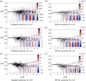
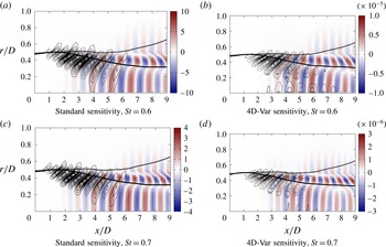
is again used as an example to explore the salient traits of the problem. Complementary results for other Strouhal numbers are shown in appendix E. In this standard sensitivity, we choose
 $\unicode[STIX]{x1D652}_{T}=0$
to be as parameter-free as possible.
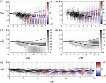
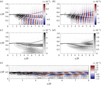
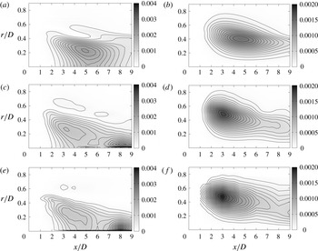
Standard sensitivity study. Superposition of the infinitesimal forcing
 $\unicode[STIX]{x1D6FF}\widetilde{\boldsymbol{f}}_{\unicode[STIX]{x1D714},m}$
(isocontours) with the associated response
 $\unicode[STIX]{x1D6FF}\widetilde{\boldsymbol{q}}_{\unicode[STIX]{x1D714},m}$
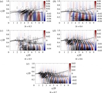
(colourmap). The critical-layer position (thick solid line) and the inflection point position (thick dashed line) are also reported on these graphs. Panel (e) respects the physical aspect ratio. (a) Real part of axial velocity. Positive contours for forcing
 $\text{Re}(\unicode[STIX]{x1D6FF}\widetilde{\boldsymbol{f}}_{\unicode[STIX]{x1D714},m}^{u})$
with solid lines, negative with dashed lines. (b) Real part of radial velocity. Positive contours for forcing
 $\text{Re}(\unicode[STIX]{x1D6FF}\widetilde{\boldsymbol{f}}_{\unicode[STIX]{x1D714},m}^{u})$
with solid lines, negative with dashed lines. (c) PSD of axial velocity. Solid lines are isocontours of forcing
 $|\unicode[STIX]{x1D6FF}\widetilde{\boldsymbol{f}}_{\unicode[STIX]{x1D714},m}^{u}|^{2}$
. Dotted lines are isocontours of the response
 $|\unicode[STIX]{x1D6FF}\widetilde{\boldsymbol{q}}_{\unicode[STIX]{x1D714},m}^{u}|^{2}$
. (d) PSD of radial velocity. Solid lines are isocontours of forcing
 $|\unicode[STIX]{x1D6FF}\widetilde{\boldsymbol{f}}_{\unicode[STIX]{x1D714},m}^{u}|^{2}$
. Dotted lines are isocontours of the response
 $|\unicode[STIX]{x1D6FF}\widetilde{\boldsymbol{q}}_{\unicode[STIX]{x1D714},m}^{u}|^{2}$
. (e) Vector field of
 $\unicode[STIX]{x1D6FF}\widetilde{\boldsymbol{f}}_{\unicode[STIX]{x1D714},m}^{u}$
, coloured by the vorticity of
 $\unicode[STIX]{x1D6FF}\widetilde{\boldsymbol{q}}_{\unicode[STIX]{x1D714},m}^{u}$
. Positive contours for forcing
 $\text{Re}(\unicode[STIX]{x1D6FF}\widetilde{\boldsymbol{f}}_{\unicode[STIX]{x1D714},m}^{u})$
with solid lines, negative with dashed lines.

Results for the forcing sensitivity
 $\unicode[STIX]{x1D6FF}\widetilde{\boldsymbol{f}}_{\unicode[STIX]{x1D714},m}$
and associated response
 $\unicode[STIX]{x1D6FF}\widetilde{\boldsymbol{q}}_{\unicode[STIX]{x1D714},m}$
for
 $\mathbb{H}(\boldsymbol{q},\unicode[STIX]{x1D6FC})=\boldsymbol{q}\text{e}^{\text{i}\int _{0}^{x}\unicode[STIX]{x1D6FC}(\unicode[STIX]{x1D709})\,\text{d}\unicode[STIX]{x1D709}}$
and
 ${\mathcal{Y}}=0$
are presented in figure 10. Since a local wavenumber of the perturbation is defined by PSE, we can draw the critical-layer position, as we did in the resolvent analysis, on
 $x$
–
 $r$
maps of forcing sensitivity and response. It can be seen in figure 10(c,d) that the highest sensitivity follows the critical layer and has a maximum value at approximately
 $x/D=3$
; we note that the locally parallel analysis also identified a maximal sensitivity at this axial station. This axial position is where the wavepacket growth rate
 $-\text{Im}(\unicode[STIX]{x1D6FC})$
becomes small (see figure 13
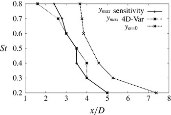
b), such that the phase speed is nearly real and a critical layer is present. Similar computations have been performed for different Strouhal numbers (see appendix E), and the axial position of the maximum value of the forcing sensitivity is reported in figure 11, compared with the axial position at which the wavepacket is neutrally stable, i.e. where
 $-\text{Im}(\unicode[STIX]{x1D6FC})=0$
. The maximum sensitivity appears systematically just upstream of the neutral position and follows the same trend. In the locally parallel analysis, the maximum sensitivity is expected for a neutral wave. Here, the mean velocity profile changes with axial position due to the jet divergence. For lower
 $x/D$
, the profile is steeper and the critical and inflection points are closer; proximity of these two points also leads to higher sensitivity to forcing, as studied in Tissot et al. (Reference Tissot, Zhang, Lajús, Cavalieri, Jordan and Colonius2015). This may explain why the maximum sensitivity appears slightly upstream of the neutral position.
Axial position
 $x_{\unicode[STIX]{x1D6FF}\widetilde{\boldsymbol{f}}_{max}}$
of the maximum forcing sensitivity
 $|\unicode[STIX]{x1D6FF}\widetilde{\boldsymbol{f}}_{\unicode[STIX]{x1D714},m}|^{2}$
(standard and 4D-Var) and axial position
 $x_{\unicode[STIX]{x1D6FC}=0}$
where the wavepacket is neutrally stable, i.e. where
 $-\text{Im}(\unicode[STIX]{x1D6FC})=0$
, function of the Strouhal number.

From
 $x/D=1$
to
 $x/D=5$
, it can be seen in figure 10(a) that the infinitesimal forcing and response are in phase; both follow the critical layer and are inclined against the shear in a manner similar to that of the OF modes of the parallel flow (figure 9). Then, from
 $x/D=5$
to
 $x/D=9$
, the forcing becomes small and the response is convected downstream. Figure 10(a,e) shows how advecting vortices are centred around the critical layer; an observation consistent with the minimum of axial velocity magnitude that follows the critical layer in figure 10(c). These inclined perturbations appear to be tilted by the shear around the critical layer as well. Moreover, figure 10(d) shows, around
 $r/D=0.5$
, a growth and decay from
 $x/D\sim 6$
to
 $x/D\sim 9$
of the PSD of the radial component of the response, while the axial component remains strong and follows the critical layer. This behaviour suggests the presence of an Orr mechanism.
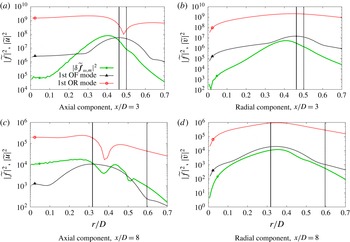
Radial profiles of the PSD. Forcing sensitivity
 $|\unicode[STIX]{x1D6FF}\widetilde{\boldsymbol{f}}_{\unicode[STIX]{x1D714},m}|^{2}$
(green bullet), the first optimal forcing mode
 $\unicode[STIX]{x1D731}_{1}$
(black triangle) and the associated response
 $\unicode[STIX]{x1D70E}_{1}\unicode[STIX]{x1D733}_{1}$
(red circle). The critical-layer position (thick solid line) and the inflection point position (thick dashed line) are also reported on these graphs.

A comparison between forcing sensitivity and response with the locally parallel resolvent analysis of § 3.2.2 can be performed. Figure 12 compares radial profiles of sensitivity
 $\unicode[STIX]{x1D6FF}\widetilde{\boldsymbol{f}}_{\unicode[STIX]{x1D714},m}$
with the optimal forcing mode
 $\unicode[STIX]{x1D731}_{1}$
and associated response
 $\unicode[STIX]{x1D70E}_{1}\unicode[STIX]{x1D733}_{1}$
at
 $x/D=3$
and
 $x/D=8$
. The first location is close to the region of peak sensitivity to forcing. The second is more characteristic of structures downstream of the potential core. A similar trend of the forcing between resolvent and PSE is shown, with maxima located near the critical layer, especially for
 $x/D=3$
. From these results we can conclude that the sensitivity analysis based on locally parallel base flows leads to general trends that are representative of the behaviour for a slowly diverging jet. At
 $x/D=8$
, the forcing is three orders of magnitude weaker. The vertical component of the forcing closely resembles the optimal forcing mode, while the axial component does not, but both peak close to the critical layer. Differences from locally parallel resolvent analysis may be attributed to cumulative effects in the streamwise direction, not accounted for in the resolvent analysis but included in PSE, which considers the entire wavepacket evolution. Disturbances thus have memory of forcing applied upstream.
The sensitivity of wavepackets predicted by PSE corroborates the results of resolvent analysis which have shown high sensitivity around the critical layer with features suggestive of an Orr mechanism. This non-parallel computation shows how the response is active downstream of the forcing locations. Small differences in comparison with the locally parallel analysis have also been noticed due to flow divergence and memory of the upstream perturbations. In order to further probe the effect of nonlinearity, we will drive this sensitivity study using the experimental data, and then push the study to convergence.
4.2.2 Sensitivity of 4D-Var
In order to explain the mismatch between linear models and experimental measurements, the sensitivity is central, but it has to be weighted by the nonlinear term actually present. With 4D-Var, by solving an inverse problem, we use the observation error to get the minimal nonlinearity sufficient to explain the mismatch.
The observations
 ${\mathcal{Y}}$
considered are the PSD of the axial and radial components of the TRPIV measurements radially filtered by POD (Cavalieri et al.
Reference Cavalieri, Rodriguez, Jordan, Colonius and Gervais2013). The observation of the axial component on the centreline,
 $\widetilde{u}_{r=0}$
, is compared in figure 13(a) with the values
 $\mathbb{H}(\boldsymbol{q},\unicode[STIX]{x1D6FC})$
predicted by PSE. It shows the good agreement of the growth of the instability wave, until this wave becomes neutrally stable at approximately
 $x/D\sim 5$
and then begins to decay, while experiments show an increase after the end of the potential core. Figure 13(b) shows the real and imaginary parts of the local wavenumber,
 $\unicode[STIX]{x1D6FC}$
, predicted by PSE.
Characterisation of the observations and of the PSE results. (a) Centerline axial fluctuating kinetic energy. Comparision between the observations
 ${\mathcal{Y}}$
(line with circles) with the PSE (dashed line) and the associated observation operator
 $\mathbb{H}(\boldsymbol{q},\unicode[STIX]{x1D6FC})$
(squares). (b) Local wavenumber predicted by PSE. Real part and imaginary part.

Figure 14(a,b) shows
 $x$
–
 $r$
maps of the observed (experimental) PSD of the axial and radial components, while figure 14(c,d) shows the axial and radial components of the homogeneous PSE solution. These plots show again how linear PSE and experiments match until approximately
 $x/D\sim 4$
. Then, looking at the PSD of the axial velocities of the observations (figure 14
a) and PSE (figure 14
c), we note that PSE has higher values around (
 $x/D=5,r/D=0.25$
) than the experiments. The experiments, on the other hand, have a significant increase of axial fluctuating kinetic energy around the centreline at
 $x/D=8$
, while PSE decays. These differences are clearly visible in the error map figure 15(a). Moreover, this error map shows that, downstream of the end of the potential core, an error follows the critical layer until the end of the domain.
Comparison between observations (first POD mode of TRPIV measurements) and PSE solution. (a)
 ${\mathcal{Y}}$
axial component. (b)
 ${\mathcal{Y}}$
radial component. (c) PSE solution, axial component of
 $|\tilde{\boldsymbol{q}}_{\unicode[STIX]{x1D714},m}|^{2}$
. (d) PSE solution, radial component of
 $|\tilde{\boldsymbol{q}}_{\unicode[STIX]{x1D714},m}|^{2}$
.

Superposition of the observation error
 $(\mathbb{H}(\boldsymbol{q},\unicode[STIX]{x1D6FC})-{\mathcal{Y}})^{2}$
(grey level and thin dotted isocontours) and the forcing sensitivity
 $|\unicode[STIX]{x1D6FF}\widetilde{\boldsymbol{f}}_{\unicode[STIX]{x1D714},m}|^{2}$
(thin solid isocontours). The dashed lines correspond also with the forcing sensitivity
 $|\unicode[STIX]{x1D6FF}\widetilde{\boldsymbol{f}}_{\unicode[STIX]{x1D714},m}|^{2}$
, but the isocontours are 10 times closer to each other in order see the smaller ‘spot’
 ${\mathcal{S}}_{2}$
. The axial component is considered. The critical-layer position (thick solid line) and the inflection point position (thick dashed line) are also reported on these graphs. In figure 15(b), the final axial position
 $L$
is chosen such that the errors near
 $x/D=8$
around the centreline are not observed. As a consequence, the near-centreline forcing
 ${\mathcal{S}}_{2}$
disappears.

In order to explore these errors, the sensitivity has been computed using the new observation space,
 $\unicode[STIX]{x1D652}_{o}=\mathbb{I}$
and
 $\unicode[STIX]{x1D652}_{T}=\unicode[STIX]{x1D70E}_{T}\mathbb{I}$
, with
 $\unicode[STIX]{x1D70E}_{T}=1$
. The terms
 $\unicode[STIX]{x1D652}_{f}$
and
 $\unicode[STIX]{x1D652}_{\unicode[STIX]{x1D702}}$
are unimportant for the sensitivity since
 $\boldsymbol{f}=0$
and
 $\boldsymbol{\unicode[STIX]{x1D702}}=0$
. Two spots of high sensitivity to forcing can be observed. Both are upstream of the locations of disagreement between linear PSE and experiments. The first, denoted
 ${\mathcal{S}}_{1}$
, peaks at approximately (
 $x/D=3,r/D=0.45$
), and is similar to the standard sensitivity presented in § 4.2.1. The second, denoted
 ${\mathcal{S}}_{2}$
, is located near the centreline at approximately
 $x/D=5$
, where the wavepacket amplitude is highest. To further explore what underlies these sensitivities, another computation is performed (results shown in figure 15
b), where the domain is truncated to
 $x_{\max }/D=7$
, such that the increase of experimental values near the centreline at
 $x/D=8$
is not observed;
 ${\mathcal{S}}_{2}$
disappears, and
 ${\mathcal{S}}_{1}$
is slightly deformed but remains qualitatively the same, showing that the small additional centreline forcing identified by 4D-Var appears to arise in order to reduce the downstream error. This suggests that even if the wavepacket is not particularly sensitive in that region, high centreline turbulent fluctuating energy near the end of the potential core contributes to reducing the downstream error. This location has been identified in the literature (Jordan & Gervais Reference Jordan and Gervais2008, and references therein) to comprise fluctuations with significant correlation with the radiated sound, but not as the source itself, as this is more consistent with a spatially extended wavepacket (Jordan & Colonius Reference Jordan and Colonius2013).
The high sensitivity at
 ${\mathcal{S}}_{1}$
is also predicted by the standard PSE sensitivity of § 4.2.1 and by the locally parallel resolvent analysis of § 3.2.2. It is interesting to see that 4D-Var also identifies this region, now considering observations, as sensitive to forcing, such that inclusion of nonlinearities would lead to improvements of model results. Figure 16 is the counterpart of figure 10 for the 4D-Var sensitivity. The similarity between the results indicates that the sensitive regions are actually excited by the background turbulence. Moreover, the position of maximum sensitivity versus
 $St$
is reported in figure 11, and the radial profiles are plotted in figure 17, showing again the same trend.
Superposition of the infinitesimal forcing
 $\unicode[STIX]{x1D6FF}\widetilde{\boldsymbol{f}}_{\unicode[STIX]{x1D714},m}$
(isocontours) with the associated response
 $\unicode[STIX]{x1D6FF}\widetilde{\boldsymbol{q}}_{\unicode[STIX]{x1D714},m}$
(colourmap). The critical-layer position (thick solid line) and the inflection point position (thick dashed line) are also reported on these graphs. Panel (e) respects the physical aspect ratio. (a) Real part of axial velocity. Positive contours for forcing
 $\text{Re}(\unicode[STIX]{x1D6FF}\widetilde{\boldsymbol{f}}_{\unicode[STIX]{x1D714},m}^{u})$
with solid lines, negative with dashed lines. (b) Real part of radial velocity. Positive contours for forcing
 $\text{Re}(\unicode[STIX]{x1D6FF}\widetilde{\boldsymbol{f}}_{\unicode[STIX]{x1D714},m}^{u})$
with solid lines, negative with dashed lines. (c) PSD of axial velocity. Solid lines are isocontours of forcing
 $|\unicode[STIX]{x1D6FF}\widetilde{\boldsymbol{f}}_{\unicode[STIX]{x1D714},m}^{u}|^{2}$
. Dotted lines are isocontours of the response
 $|\unicode[STIX]{x1D6FF}\widetilde{\boldsymbol{q}}_{\unicode[STIX]{x1D714},m}^{u}|^{2}$
. (d) PSD of radial velocity. Solid lines are isocontours of forcing
 $|\unicode[STIX]{x1D6FF}\widetilde{\boldsymbol{f}}_{\unicode[STIX]{x1D714},m}^{v}|^{2}$
. Dotted lines are isocontours of the response
 $|\unicode[STIX]{x1D6FF}\widetilde{\boldsymbol{q}}_{\unicode[STIX]{x1D714},m}^{v}|^{2}$
. (e) Vector field of
 $\unicode[STIX]{x1D6FF}\widetilde{\boldsymbol{q}}_{\unicode[STIX]{x1D714},m}$
, colored by the vorticity of
 $\unicode[STIX]{x1D6FF}\widetilde{\boldsymbol{q}}_{\unicode[STIX]{x1D714},m}$
. Positive contours for forcing
 $\text{Re}(\unicode[STIX]{x1D6FF}\widetilde{\boldsymbol{f}}_{\unicode[STIX]{x1D714},m}^{u})$
with solid lines, negative with dashed lines.

Radial profiles of the PSD of the axial component: observations
 ${\mathcal{Y}}$
(blue squares), PSE (black dashed line), forcing sensitivity
 $|\unicode[STIX]{x1D6FF}\widetilde{\boldsymbol{f}}_{\unicode[STIX]{x1D714},m}|^{2}$
(green bullet), the first optimal forcing mode
 $\unicode[STIX]{x1D731}_{1}$
(black triangle) and the associated response
 $\unicode[STIX]{x1D70E}_{1}\unicode[STIX]{x1D733}_{1}$
(red circle). The critical-layer position (thick solid line) and the inflection point position (thick dashed line) are also reported on these graphs.

Comparison between observations (first POD mode of TRPIV measurements), homogeneous PSE solution and PSE solution forced by 4D-Var for
 $St=0.6$
. (a) Homogeneous PSE solution, axial component of
 $|\tilde{\boldsymbol{q}}_{\unicode[STIX]{x1D714},m}|^{2}$
. (b) Homogeneous PSE solution, radial component of
 $|\tilde{\boldsymbol{q}}_{\unicode[STIX]{x1D714},m}|^{2}$
. (c) Forced PSE solution, axial component of
 $|\tilde{\boldsymbol{q}}_{\unicode[STIX]{x1D714},m}|^{2}$
. (d) Forced PSE solution, radial component of
 $|\tilde{\boldsymbol{q}}_{\unicode[STIX]{x1D714},m}|^{2}$
. (e)
 ${\mathcal{Y}}$
axial component. (f)
 ${\mathcal{Y}}$
radial component.

The response (figure 16 c) and the error (figure 15 a) can be directly compared; their correspondence shows that the response actually decreases the error. The observed mechanism can be described as follows: nonlinearities induce disturbances inclined against the shear in the critical-layer region; advection of such disturbances leads to a tilting of structures with an amplitude growth characteristic of the Orr mechanism; this growth increases amplitudes in the downstream region, and wavepacket amplitudes get closer to experimental results.
All of the results presented in this section are for
 $St=0.6$
, but other Strouhal numbers display the same trends. Some results for other Strouhal numbers are shown in appendix E, and are consistent with the phenomena described here, with some minor differences.
To summarise, the PSE-4D-Var reveals that a high sensitivity to forcing at approximately
 $x/D=3$
promotes the generation of convected perturbations that decrease the error between PSE and experiment at the end of the potential core. This mechanism is consistent with the locally parallel results and is believed to be associated with the critical layer. Downstream of the potential core, results suggest that an Orr mechanism may be active around the critical layer, tilting the structures and generating a growth and decay of the PSD of the radial velocity. The results suggest that nonlinearities may act on wavepackets via this mechanism, with significant effects in the downstream region. Another important region was found on the jet centreline, close to the end of the potential core. This region did not show high sensitivity to forcing in the previous section. Since PSE-4D-Var determines forcings that minimise the error between model and reference measurements, the results suggest that high-amplitude forcings (i.e. significant nonlinear effects) are present in the identified region.
4.2.3 Convergence to experimental results
The solution of the minimisation of (4.7) is the minimal nonlinear term necessary to best approach the measurements. We now solve this problem by iterating the direct/adjoint procedure until convergence. A steepest descent algorithm is used with a backtracking Armijo-type linsearch method. The covariance matrices are chosen as
 $\unicode[STIX]{x1D652}_{o}=\mathbb{I}$
,
 $\unicode[STIX]{x1D652}_{\unicode[STIX]{x1D702}}=\unicode[STIX]{x1D70E}_{\unicode[STIX]{x1D702}}\mathbb{I}$
,
 $\unicode[STIX]{x1D652}_{f}=\unicode[STIX]{x1D70E}_{f}\mathbb{I}$
and
 $\unicode[STIX]{x1D652}_{T}=\unicode[STIX]{x1D70E}_{T}\mathbb{I}$
, with
 $\unicode[STIX]{x1D70E}_{f}=\unicode[STIX]{x1D70E}_{\unicode[STIX]{x1D702}}=1$
and
 $\unicode[STIX]{x1D70E}_{T}=10^{-2}$
. These values have been determined by the L-curve method (Hansen Reference Hansen1992; Cordier, El Majd & Favier Reference Cordier, El Majd and Favier2010).
Figure 18 compares homogeneous PSE, forced PSE and measurements for
 $St=0.6$
, showing that the forcing is successful in producing waves with PSD that match those of the experiments.
The forcing
 $\widetilde{\boldsymbol{f}}_{\unicode[STIX]{x1D714},m}$
and the response
 $\unicode[STIX]{x1D6FF}\widetilde{\boldsymbol{q}}_{\unicode[STIX]{x1D714},m}=\widetilde{\boldsymbol{q}}_{\unicode[STIX]{x1D714},m}^{f}-\widetilde{\boldsymbol{q}}_{\unicode[STIX]{x1D714},m}^{h}$
are plotted in figure 19. The forcing magnitude is approximately
 $10\,\%$
of the wavepacket amplitude, which is significant but remains small. From a reduced-order-modelling perspective, the relatively low amplitude of the required forcing suggests that linear wavepacket models might be substantially improved, in terms of agreement with experiment, by slight modifications via the inclusion of some relevant nonlinear interactions.
The forcing shape is more complex than what was found in the sensitivity analyses, but it possesses the same features. A high-amplitude forcing follows the critical layer, and another important forcing region is concentrated around the centreline. There is, moreover, a third region of relevant forcing that appears to follow the inflection point but vanishes quickly. The two major differences compared with the 4D-Var sensitivity of § 4.2.2 are that the forcing continues along the critical layer much further downstream, and the centreline forcing is as large as the critical-layer forcing, while it is one order of magnitude less for the 4D-Var sensitivity. The downstream continuation of the forcing can be explained by the fact that as long as the forcing excites the wavepacket, nearly neutral growth of amplitudes can be sustained. A critical layer is then still present and the wavepacket continues to be sensitive to turbulence. This scenario remains plausible since high turbulent levels are still present at these downstream stations. Since wavy disturbances are continuously excited while propagating downstream, the tilting of structures by an Orr-like mechanism is a little less clear in figure 19 than in the sensitivity study, but the overall trend can still be perceived. Concerning the strong centreline forcing, the present result confirms the analysis that even though the wavepacket is not particularly sensitive near the centreline, it has to be forced there in order to lead to the observed experimental amplitudes.
Superposition of the converged 4D-Var forcing
 $\unicode[STIX]{x1D6FF}\widetilde{\boldsymbol{f}}_{\unicode[STIX]{x1D714},m}$
(isocontours) with the associated response
 $\unicode[STIX]{x1D6FF}\widetilde{\boldsymbol{q}}_{\unicode[STIX]{x1D714},m}=\widetilde{\boldsymbol{q}}_{\unicode[STIX]{x1D714},m}^{f}-\widetilde{\boldsymbol{q}}_{\unicode[STIX]{x1D714},m}^{h}$
(colourmap); real part of the axial velocity; positive contours for forcing
 $\text{Re}(\widetilde{\boldsymbol{f}}_{\unicode[STIX]{x1D714},m}^{u})$
with solid lines, negative with dashed lines. The critical-layer position (thick solid line) and the inflection point position (thick dashed line) are also reported. The physical aspect ratio is respected.

Finally, the observation errors seem to be insensitive to the inflow initial condition (sensitivity not plotted), which is probably a consequence of the dominance of the K–H mode in the upstream region and a fast decay of all of the other modes.
We have learnt by converging 4D-Var that the minimal forcing excites the wavepacket along the critical layer throughout its evolution, which, in the downstream region, maintains nearly constant disturbance amplitudes as these are advected. Moreover, detection of a relevant forcing near the centreline, despite the relatively low sensitivity of this region to external forcing, suggests the presence of strong active turbulence in that region, capable of considerably influencing wavepacket evolution.
5 Conclusion
We have considered the effect of nonlinearities on wavepackets in jets. Representing the nonlinear term as a harmonic, ‘external’ forcing acting on the linearised operator is found to be a useful means by which to incorporate nonlinearity in standard linear wavepacket models. The response of such models to forcing has been computed and compared with available experimental data, and forced-wavepacket signatures thus confirmed downstream of the end of the potential core, where linear models fail. By considering problems of varying degrees of complexity, the sensitivity of the linear operator to such forcing is shown to be systematically maximal at the critical layer, indicating that this plays a central role.
Optimal forcing modes and corresponding flow responses, predicted by a locally parallel resolvent analysis, were shown to dominate the input–output behaviour of the linearised operator, and also to display traits typical of a critical-layer mechanism. A maximum sensitivity at approximately
 $x/D=3$
, upstream of the end of the potential core, is predicted by the locally parallel resolvent analysis and subsequently confirmed, in a non-parallel framework, by a sensitivity analysis performed using PSE-4D-Var. This last method was introduced in this work in order to account for slowly diverging base flows, and determine missing nonlinear forcing terms such that results of linear models would approach measurements. The PSE-4DVar approach, by correctly including non-parallel effects, permits analysis of the convection of the response in the axial direction. This method has been used in a pure sensitivity analysis, in a sensitivity analysis driven by the discrepancy between PSE and data, and, finally, for resolution of the associated optimisation problem. One large discrepancy between homogeneous linear PSE and measurements, downstream of the end of the potential core, has been associated with this highly sensitive zone (at approximately
 $x/D=3$
). When full optimisation is performed, this zone extends downstream. Results suggest that the response to the identified forcing in PSE-4D-Var is driven around the critical layer by an Orr-like mechanism continuously sustained by turbulence.
The critical layer appears thus to play a central role in the forced-wavepacket scenario considered, acting in two ways. The first involves providing a high sensitivity for nonlinear forcing; whenever such forcing has a phase speed matching the local mean-flow velocity, it excites significant disturbance amplitudes. The second is manifested in the tilting of perturbations, which are advected at the local flow velocity with corresponding amplitude growth via the Orr mechanism.
Moreover, we have identified another region where forcing is relevant, near the centreline. In this region, the wavepacket is not particularly sensitive, but the forcing permits a better match with the measurements, suggesting the presence of significant turbulent nonlinear interactions exciting the wavepacket.
From a reduced-order-modelling perspective, the optimal forcing modes, identified in a locally parallel framework, are good candidates for the modelling of nonlinearities. The optimal response mode dominates, suggesting that single-mode representations might be sufficient for modelling purposes. Before building a nonlinear autonomous model, however, it is necessary to discern how nonlinearities in the jet project onto these modes. This complementary issue, which is presently being explored, is central for identification of the essential features necessary for prediction of wavepacket dynamics. It will allow the generation of a balanced basis of nonlinear structures, which are both present in the jet and highly amplified by the linearised operator.
Finally, for the problem of sound radiation of subsonic turbulent jets considered here, the coherence decay would appear to be a key property to be matched by nonlinear wavepacket models (Cavalieri & Agarwal Reference Cavalieri and Agarwal2014), if jitter (Cavalieri et al. Reference Cavalieri, Daviller, Comte, Jordan, Tadmor and Gervais2011a ) and quantitatively accurate sound predictions are to be obtained. Because a harmonic analysis was considered in this work, a perfectly coherent forcing is obtained by PSE-4D-Var and resolvent analyses. Knowledge of the responses of the linear operator to nonlinear forcing terms is nonetheless an important step in the understanding of how nonlinearities affect coherence decay and sound radiation. Additional post-processing will be considered in further work, in the spirit of Baqui et al. (Reference Baqui, Agarwal, Cavalieri and Sinayoko2015), to exploit the optimal solution for acoustic prediction.
Acknowledgements
We thank T. Colonius for advice and fruitful discussions during the course of the research reported here. We also thank K. Sasaki for his contribution to the development of the PSE code. This work was supported by the program Science Without Borders (project A073/2013), the ANR project COOLJAZZ and through funding from the Fondation Université de Poitiers.
Appendix A. The full set of equations used in the resolvent analysis
For completeness, in this appendix we present the full equations of the homogeneous linearised Navier–Stokes system for an axisymmetric disturbance (
 $m=0$
), used in the resolvent analysis. The equations are written in terms of (
 $\widetilde{u},\widetilde{v},\widetilde{\unicode[STIX]{x1D70C}},\widetilde{T}$
) in cylindrical coordinates.
Equation for
 $x$
-momentum:
 $$\begin{eqnarray}\displaystyle & & \displaystyle \!\!\!-\text{i}\unicode[STIX]{x1D714}\widetilde{u}+\text{i}\unicode[STIX]{x1D6FC}\bar{U}\widetilde{u}+\widetilde{v}\bar{U}^{\prime }=-\frac{\unicode[STIX]{x1D6FE}-1}{\unicode[STIX]{x1D6FE}}\text{i}\unicode[STIX]{x1D6FC}\widetilde{T}-\frac{\unicode[STIX]{x1D6FE}-1}{\unicode[STIX]{x1D6FE}}\frac{\bar{T}}{\bar{\unicode[STIX]{x1D70C}}}\text{i}\unicode[STIX]{x1D6FC}\widetilde{\unicode[STIX]{x1D70C}}\nonumber\\ \displaystyle & & \displaystyle \quad +\,\frac{1}{\bar{\unicode[STIX]{x1D70C}}Re}\left[\bar{\unicode[STIX]{x1D707}}\left(-\unicode[STIX]{x1D6FC}^{2}\widetilde{u}+\frac{1}{r}\frac{\unicode[STIX]{x2202}}{\unicode[STIX]{x2202}r}\left(r\frac{\unicode[STIX]{x2202}\widetilde{u}}{\unicode[STIX]{x2202}r}\right)\right)+\frac{\bar{\unicode[STIX]{x1D707}}}{3}\left(-\unicode[STIX]{x1D6FC}^{2}\widetilde{u}+\text{i}\unicode[STIX]{x1D6FC}\frac{\unicode[STIX]{x2202}\widetilde{v}}{\unicode[STIX]{x2202}r}+\frac{\text{i}\unicode[STIX]{x1D6FC}}{r}\widetilde{v}\right)\right.\nonumber\\ \displaystyle & & \displaystyle \quad +\,\frac{\unicode[STIX]{x2202}\bar{\unicode[STIX]{x1D707}}}{\unicode[STIX]{x2202}r}\left.\!\left(\text{i}\unicode[STIX]{x1D6FC}\widetilde{v}+\frac{\unicode[STIX]{x2202}\widetilde{u}}{\unicode[STIX]{x2202}r}\right)+\frac{\unicode[STIX]{x1D707}}{r}\frac{\unicode[STIX]{x2202}}{\unicode[STIX]{x2202}r}\left(r\frac{\unicode[STIX]{x2202}\bar{U}}{\unicode[STIX]{x2202}r}\right)+\frac{\unicode[STIX]{x2202}\unicode[STIX]{x1D707}}{\unicode[STIX]{x2202}r}\frac{\unicode[STIX]{x2202}\bar{U}}{\unicode[STIX]{x2202}r}+\bar{\unicode[STIX]{x1D707}}_{B}\left(\!-\unicode[STIX]{x1D6FC}^{2}\widetilde{u}+\text{i}\unicode[STIX]{x1D6FC}\frac{\unicode[STIX]{x2202}\widetilde{v}}{\unicode[STIX]{x2202}r}+\frac{\text{i}\unicode[STIX]{x1D6FC}}{r}\widetilde{v}\right)\right].\hspace{-5.0pt}\nonumber\\ \displaystyle & & \displaystyle\end{eqnarray}$$
Equation for
 $r$
-momentum:
 $$\begin{eqnarray}\displaystyle & & \displaystyle -\text{i}\unicode[STIX]{x1D714}\widetilde{v}+\text{i}\unicode[STIX]{x1D6FC}\bar{U}\widetilde{v}=-\frac{\unicode[STIX]{x1D6FE}-1}{\unicode[STIX]{x1D6FE}}\frac{\unicode[STIX]{x2202}\widetilde{T}}{\unicode[STIX]{x2202}r}-\frac{\unicode[STIX]{x1D6FE}-1}{\unicode[STIX]{x1D6FE}}\frac{\bar{T}}{\bar{\unicode[STIX]{x1D70C}}}\frac{\unicode[STIX]{x2202}\widetilde{\unicode[STIX]{x1D70C}}}{\unicode[STIX]{x2202}r}-\frac{\unicode[STIX]{x1D6FE}-1}{\unicode[STIX]{x1D6FE}}\frac{\widetilde{\unicode[STIX]{x1D70C}}}{\bar{\unicode[STIX]{x1D70C}}}\frac{\unicode[STIX]{x2202}\bar{T}}{\unicode[STIX]{x2202}r}-\frac{\unicode[STIX]{x1D6FE}-1}{\unicode[STIX]{x1D6FE}}\frac{\widetilde{T}}{\bar{\unicode[STIX]{x1D70C}}}\frac{\unicode[STIX]{x2202}\bar{\unicode[STIX]{x1D70C}}}{\unicode[STIX]{x2202}r}\nonumber\\ \displaystyle & & \displaystyle \quad +\,\frac{1}{\bar{\unicode[STIX]{x1D70C}}Re}\left[\bar{\unicode[STIX]{x1D707}}\left(-\unicode[STIX]{x1D6FC}^{2}\widetilde{v}+\frac{1}{r}\frac{\unicode[STIX]{x2202}}{\unicode[STIX]{x2202}r}\left(r\frac{\unicode[STIX]{x2202}\widetilde{v}}{\unicode[STIX]{x2202}r}\right)\right)+\frac{\bar{\unicode[STIX]{x1D707}}}{3}\left(\text{i}\unicode[STIX]{x1D6FC}\frac{\unicode[STIX]{x2202}\widetilde{u}}{\unicode[STIX]{x2202}r}+\frac{\unicode[STIX]{x2202}^{2}\widetilde{v}}{\unicode[STIX]{x2202}r^{2}}+\frac{1}{r}\frac{\unicode[STIX]{x2202}\widetilde{v}}{\unicode[STIX]{x2202}r}-\frac{\widetilde{v}}{r^{2}}\right)\right.\nonumber\\ \displaystyle & & \displaystyle \quad -\,\frac{\bar{\unicode[STIX]{x1D707}}\widetilde{v}}{r^{2}}+\frac{\unicode[STIX]{x2202}\bar{\unicode[STIX]{x1D707}}}{\unicode[STIX]{x2202}r}\left(2\frac{\unicode[STIX]{x2202}\widetilde{v}}{\unicode[STIX]{x2202}r}-\frac{2\text{i}\unicode[STIX]{x1D6FC}}{3}\widetilde{u}-\frac{2}{3}\frac{\unicode[STIX]{x2202}\widetilde{v}}{\unicode[STIX]{x2202}r}-\frac{2}{3}\frac{\widetilde{v}}{r}\right)+\text{i}\unicode[STIX]{x1D6FC}\unicode[STIX]{x1D707}\bar{U}^{\prime }\nonumber\\ \displaystyle & & \displaystyle \quad +\,\bar{\unicode[STIX]{x1D707}}_{B}\left.\left(\text{i}\unicode[STIX]{x1D6FC}\frac{\unicode[STIX]{x2202}\widetilde{u}}{\unicode[STIX]{x2202}r}+\frac{\unicode[STIX]{x2202}^{2}\widetilde{v}}{\unicode[STIX]{x2202}r^{2}}+\frac{1}{r}\frac{\unicode[STIX]{x2202}\widetilde{v}}{\unicode[STIX]{x2202}r}-\frac{\widetilde{v}}{r^{2}}\right)+\frac{\unicode[STIX]{x2202}\bar{\unicode[STIX]{x1D707}}_{B}}{\unicode[STIX]{x2202}r}\left(\text{i}\unicode[STIX]{x1D6FC}\widetilde{u}+\frac{\unicode[STIX]{x2202}\widetilde{v}}{\unicode[STIX]{x2202}r}+\frac{\widetilde{v}}{r}\right)\right].\end{eqnarray}$$
Continuity equation:
 $$\begin{eqnarray}\displaystyle -\!\text{i}\unicode[STIX]{x1D714}\widetilde{\unicode[STIX]{x1D70C}}+\text{i}\unicode[STIX]{x1D6FC}\bar{U}\widetilde{\unicode[STIX]{x1D70C}}+\bar{\unicode[STIX]{x1D70C}}\text{i}\unicode[STIX]{x1D6FC}\widetilde{u}+\bar{\unicode[STIX]{x1D70C}}\frac{\unicode[STIX]{x2202}\widetilde{v}}{\unicode[STIX]{x2202}r}+\widetilde{v}\frac{\unicode[STIX]{x2202}\bar{\unicode[STIX]{x1D70C}}}{\unicode[STIX]{x2202}r}+\frac{\bar{\unicode[STIX]{x1D70C}}\widetilde{v}}{r}=0. & & \displaystyle\end{eqnarray}$$
Energy equation:
 $$\begin{eqnarray}\displaystyle & & \displaystyle -\text{i}\unicode[STIX]{x1D714}\widetilde{T}+\widetilde{v}\frac{\unicode[STIX]{x2202}\bar{T}}{\unicode[STIX]{x2202}r}+\text{i}\unicode[STIX]{x1D6FC}\bar{U}\widetilde{T}+(\unicode[STIX]{x1D6FE}-1)\bar{T}\left(\text{i}\unicode[STIX]{x1D6FC}\widetilde{u}+\frac{\unicode[STIX]{x2202}\widetilde{v}}{\unicode[STIX]{x2202}r}+\frac{\widetilde{v}}{r}\right)\nonumber\\ \displaystyle & & \displaystyle \quad =\frac{\unicode[STIX]{x1D6FE}}{\bar{\unicode[STIX]{x1D70C}}RePr}\left[\bar{\unicode[STIX]{x1D707}}\left(-\unicode[STIX]{x1D6FC}^{2}\widetilde{T}+\frac{\unicode[STIX]{x2202}^{2}\widetilde{T}}{\unicode[STIX]{x2202}r^{2}}+\frac{1}{r}\frac{\unicode[STIX]{x2202}\widetilde{T}}{\unicode[STIX]{x2202}r}\right)+\unicode[STIX]{x1D707}\left(\frac{\unicode[STIX]{x2202}^{2}\bar{T}}{\unicode[STIX]{x2202}r^{2}}+\frac{1}{r}\frac{\unicode[STIX]{x2202}\bar{T}}{\unicode[STIX]{x2202}r}\right)+\frac{\unicode[STIX]{x2202}\bar{\unicode[STIX]{x1D707}}}{\unicode[STIX]{x2202}r}\frac{\unicode[STIX]{x2202}\widetilde{T}}{\unicode[STIX]{x2202}r}+\frac{\unicode[STIX]{x2202}\unicode[STIX]{x1D707}}{\unicode[STIX]{x2202}r}\frac{\unicode[STIX]{x2202}\bar{T}}{\unicode[STIX]{x2202}r}\right]\nonumber\\ \displaystyle & & \displaystyle \qquad +\,\frac{\unicode[STIX]{x1D6FE}}{\bar{\unicode[STIX]{x1D70C}}}\left[\frac{2\bar{\unicode[STIX]{x1D707}}}{Re}\frac{\unicode[STIX]{x2202}\bar{U}}{\unicode[STIX]{x2202}r}\left(\text{i}\unicode[STIX]{x1D6FC}\widetilde{v}+\frac{\unicode[STIX]{x2202}\widetilde{u}}{\unicode[STIX]{x2202}r}\right)+\frac{\unicode[STIX]{x1D707}}{Re}\left(\frac{\unicode[STIX]{x2202}\bar{U}}{\unicode[STIX]{x2202}r}\right)^{2}\right].\end{eqnarray}$$
Appendix B. Selection of the phase velocity in the resolvent analysis
In the locally parallel resolvent analysis, the phase velocity of the perturbation is a free parameter. In this work, we focus on real-valued phase velocities, since we are interested in quasi-neutral waves excited by turbulence downstream of the end of the potential core.
Values of the phase speed and
 $|\unicode[STIX]{x1D6FD}_{RA-TRPIV}|$
metric, defined in (3.8), measuring the agreement between the optimal response mode and measurements, are displayed in figure 20 for three different choices of
 $c$
. We first choose at each axial position
 $c$
that maximises
 $|\unicode[STIX]{x1D6FD}_{RA-TRPIV}|$
. It is the optimal value, used here as a reference for the maximum possible agreement with experimental results. We then choose
 $c$
to be either the real part of the value predicted by homogeneous PSE or the value leading to the maximum energy gain
 $\unicode[STIX]{x1D70E}_{i}^{2}$
.
The effect of phase velocity on agreement between TRPIV and the resolvent analysis. (a) Phase velocity
 $c$
chosen to maximise
 $|\unicode[STIX]{x1D6FD}_{RA\text{-}TRPIV}|$
. (b) Optimal
 $|\unicode[STIX]{x1D6FD}_{RA\text{-}TRPIV}|$
metric. (c) Phase velocity
 $c$
determined by PSE. (d)
 $|\unicode[STIX]{x1D6FD}_{RA\text{-}TRPIV}|$
metric for
 $c$
determined by PSE. (e) Phase velocity
 $c$
chosen to maximise the optimal energy gain
 $\unicode[STIX]{x1D70E}_{i}^{2}$
. (f)
 $|\unicode[STIX]{x1D6FD}_{RA\text{-}TRPIV}|$
metric for
 $c$
chosen to maximise the optimal energy gain
 $\unicode[STIX]{x1D70E}_{i}^{2}$
.

It can be seen that the values of
 $|\unicode[STIX]{x1D6FD}_{RA-TRPIV}|$
for
 $c$
determined by PSE are quite close to the optimal ones, while the values of
 $|\unicode[STIX]{x1D6FD}_{RA-TRPIV}|$
for
 $c$
maximising
 $\unicode[STIX]{x1D70E}_{i}^{2}$
lead to worse agreement (lower
 $|\unicode[STIX]{x1D6FD}|$
) with experimental results. Use of the phase speed given by PSE seems then to be a good choice.
Beyond the choice of the phase speed, the above result is informative of phenomena at play. A resolvent analysis based on a PSE-predicted phase speed represents the study of the response of the wavepacket to external turbulent forcing. On the other hand, a maximum energy gain would study the generation of a new wave, eventually with completely different phase speed, by turbulence. We have found that the former is more representative of the data than the latter, which is in line with the hypotheses of the present study.
Appendix C. Complementary results of the resolvent analysis
In this appendix, a complete view of the resolvent analysis is given. Figure 21 compares for a range of axial positions
 $x/D=[2-9]$
the PSD of the axial velocity fluctuation measured by TRPIV, predicted by PSE and of the optimal response modes. The corresponding phases are shown in figure 22.
Comparison of optimal forcing (red dashed lines) and the optimal response modes (red solid lines) of axial velocity fluctuation at
 $x/D=2{-}9$
with experimental data (blue squares) and the solution of the homogeneous linear problem (LEE, green line with solid dots; PSE, black dashed line). Here,
 $St=0.6,Re=10\,000$
,
 $M=0.4$
;
 $c$
is determined from the PSE calculation. The vertical dashed line is the critical-layer position and the vertical dash-dotted line is the inflectional point position.

As mentioned in the text, PSE and LEE begin to get away from measurements at
 $x/D=5$
, while the optimal response continues to have a dip in amplitude at a radial position close to the experimental one. The optimal forcing systematically has a maximum at the critical layer.
Comparison of the shifted phases of axial velocity fluctuation at
 $x/D=2{-}9$
: OR of resolvent analysis, squares; TRPIV, line; PSE, crosses. The phases are shifted to have zero reference phase at
 $r/D=0$
. Here,
 $St=0.6,Re=10000,M=0.4$
and PSE-determined
 $c$
. The two horizontal dashed lines are at
 $-\unicode[STIX]{x03C0}$
and
 $\unicode[STIX]{x03C0}$
. The vertical dashed line is the critical-layer position (according to the PSE solution) and the vertical dash-dotted line is the inflectional point position.

For the TRPIV and OR profiles, the phase jump shown in figure 22 is systematically a
 $\unicode[STIX]{x03C0}$
jump, a sign of a vortex-like structure. Experiments and PSE predict a smooth change of the phase. At downstream stations, phases from PSE have an increasing mismatch with experimental values. The modes from the resolvent analysis present a sharper jump, but closer to the experimental results for downstream stations.
Appendix D. Derivation of gradient of PSE-4D-Var
In this appendix, we will detail the derivation of the Lagrangian in the case of the cost functional minimising the error between PSE and experiments according to (4.9). In the case of the standard sensitivity, the distinction will be made only for the final result.
In order to obtain the optimality system (4.11), (4.12) and (4.13), we have to derive the Lagrangian (4.10a
)–(4.10c
) with respect to each variable. We denote by
 $\unicode[STIX]{x1D735}_{\unicode[STIX]{x1D753}}{\mathcal{L}}$
the gradient of
 ${\mathcal{L}}$
with respect to a variable
 $\unicode[STIX]{x1D753}$
, defined such that for any variation
 $\unicode[STIX]{x1D6FF}\unicode[STIX]{x1D753}$
, we have
 $$\begin{eqnarray}\displaystyle (\unicode[STIX]{x1D735}_{\unicode[STIX]{x1D753}}{\mathcal{L}},\unicode[STIX]{x1D6FF}\unicode[STIX]{x1D753})_{\unicode[STIX]{x1D753}}=\lim _{\unicode[STIX]{x1D716}\rightarrow 0}\frac{{\mathcal{L}}(\unicode[STIX]{x1D753}+\unicode[STIX]{x1D716}\unicode[STIX]{x1D6FF}\unicode[STIX]{x1D753})-{\mathcal{L}}(\unicode[STIX]{x1D753})}{\unicode[STIX]{x1D716}}. & & \displaystyle\end{eqnarray}$$
The inner product
 $(\cdot \,,\cdot )_{\unicode[STIX]{x1D753}}$
is the inner product in the space where
 $\unicode[STIX]{x1D753}$
lies. For PSE, we define three different inner products:
 $$\begin{eqnarray}\displaystyle & \displaystyle (a,b)_{x}=\int _{0}^{L}a(x)b(x)\,\text{d}x, & \displaystyle\end{eqnarray}$$
 $$\begin{eqnarray}\displaystyle & \displaystyle (a,b)_{r}=\int _{0}^{\infty }a(r)b(r)r\,\text{d}r, & \displaystyle\end{eqnarray}$$
 $$\begin{eqnarray}\displaystyle & \displaystyle (a,b)_{xr}=\int _{0}^{L}\int _{0}^{\infty }a(x,r)b(x,r)r\,\text{d}r\,\text{d}x=\int _{0}^{L}(a,b)_{r}\,\text{d}x. & \displaystyle\end{eqnarray}$$
D.1 Directional derivative in the directions
 $\unicode[STIX]{x1D6FF}\unicode[STIX]{x1D740}$
,
$\unicode[STIX]{x1D6FF}\unicode[STIX]{x1D701}$
and
$\unicode[STIX]{x1D6FF}\unicode[STIX]{x1D743}$


Using the definition (D 1), we obtain
 $$\begin{eqnarray}\displaystyle & \displaystyle (\unicode[STIX]{x1D735}_{\unicode[STIX]{x1D740}}{\mathcal{L}},\unicode[STIX]{x1D6FF}\unicode[STIX]{x1D740})_{xr}=-\text{Re}\left(\int _{0}^{L}\left(\unicode[STIX]{x1D640}\frac{\unicode[STIX]{x2202}\boldsymbol{q}}{\unicode[STIX]{x2202}x}+(\unicode[STIX]{x1D63C}+\unicode[STIX]{x1D6FC}\unicode[STIX]{x1D63E})\boldsymbol{q}-\boldsymbol{w},\unicode[STIX]{x1D6FF}\unicode[STIX]{x1D740}\right)_{r}\,\text{d}x\right), & \displaystyle\end{eqnarray}$$
 $$\begin{eqnarray}\displaystyle & \displaystyle (\unicode[STIX]{x1D735}_{\unicode[STIX]{x1D701}}{\mathcal{L}},\unicode[STIX]{x1D6FF}\unicode[STIX]{x1D701})_{x}=-\text{Re}\left(\int _{0}^{L}\left(\boldsymbol{q},\frac{\unicode[STIX]{x2202}\boldsymbol{q}}{\unicode[STIX]{x2202}x}\right)_{r}\unicode[STIX]{x1D6FF}\unicode[STIX]{x1D701}\,\text{d}x\right), & \displaystyle\end{eqnarray}$$
 $$\begin{eqnarray}\displaystyle & \displaystyle (\unicode[STIX]{x1D735}_{\unicode[STIX]{x1D743}}{\mathcal{L}},\unicode[STIX]{x1D6FF}\unicode[STIX]{x1D743})_{r}=-\text{Re}((\boldsymbol{q}(0,r)-\boldsymbol{q}_{0}-\boldsymbol{\unicode[STIX]{x1D702}},\unicode[STIX]{x1D6FF}\unicode[STIX]{x1D743})_{r}). & \displaystyle\end{eqnarray}$$
 $\unicode[STIX]{x1D735}_{\unicode[STIX]{x1D740}}{\mathcal{L}}=\unicode[STIX]{x1D735}_{\unicode[STIX]{x1D701}}{\mathcal{L}}=\unicode[STIX]{x1D735}_{\unicode[STIX]{x1D743}}{\mathcal{L}}=0$
for each
 $\unicode[STIX]{x1D6FF}\unicode[STIX]{x1D740}$
,
 $\unicode[STIX]{x1D6FF}\unicode[STIX]{x1D701}$
and
 $\unicode[STIX]{x1D6FF}\unicode[STIX]{x1D743}$
. The direct system (4.11) is then a part of the optimality system. As a consequence, when the minimum is reached, we also have
 ${\mathcal{J}}={\mathcal{L}}$
.
D.2 Directional derivative in the directions
$\unicode[STIX]{x1D6FF}\boldsymbol{q}$

Because the derivation is long, we will treat the different terms (4.10a )–(4.10d ) separately.
Term (4.10a ):
 $$\begin{eqnarray}\displaystyle & & \displaystyle \!\!\!\!(\unicode[STIX]{x1D735}_{\boldsymbol{q}}{\mathcal{L}},\unicode[STIX]{x1D6FF}\boldsymbol{q})_{xr}^{(4.10a)}=\lim _{\unicode[STIX]{x1D716}\rightarrow 0}\frac{1}{\unicode[STIX]{x1D716}}\text{ Re}\left(\int _{0}^{L}\!(\unicode[STIX]{x1D64C}(|\boldsymbol{q}+\unicode[STIX]{x1D716}\unicode[STIX]{x1D6FF}\boldsymbol{q}|^{2}-|\boldsymbol{q}|^{2})|\text{e}^{\text{i}\int _{0}^{x}\unicode[STIX]{x1D6FC}(\unicode[STIX]{x1D709})\,\text{d}\unicode[STIX]{x1D709}}|^{2},\mathbb{H}(\boldsymbol{q},\unicode[STIX]{x1D6FC})-{\mathcal{Y}})_{\unicode[STIX]{x1D652}_{o}}\,\text{d}x\!\right)\nonumber\\ \displaystyle & & \displaystyle \qquad +\,\lim _{\unicode[STIX]{x1D716}\rightarrow 0}\frac{1}{\unicode[STIX]{x1D716}}\text{ Re}((\unicode[STIX]{x1D64C}(|\boldsymbol{q}_{L}+\unicode[STIX]{x1D716}\unicode[STIX]{x1D6FF}\boldsymbol{q}_{L}|^{2}-|\boldsymbol{q}_{L}|^{2})|\text{e}^{\text{i}\int _{0}^{L}\unicode[STIX]{x1D6FC}(\unicode[STIX]{x1D709})\,\text{d}\unicode[STIX]{x1D709}}|^{2},\mathbb{H}(\boldsymbol{q}_{L},\unicode[STIX]{x1D6FC}_{L})-{\mathcal{Y}}_{L})_{\unicode[STIX]{x1D652}_{T}})\nonumber\\ \displaystyle & & \displaystyle \quad =\text{Re}\left(\int _{0}^{L}(\unicode[STIX]{x1D6FF}\boldsymbol{q},2|\text{e}^{\text{i}\int _{0}^{x}\unicode[STIX]{x1D6FC}(\unicode[STIX]{x1D709})\,\text{d}\unicode[STIX]{x1D709}}|^{2}((\unicode[STIX]{x1D64C}^{\ast }\unicode[STIX]{x1D64C}\unicode[STIX]{x1D63F}_{\bar{\boldsymbol{q}}})^{+}\unicode[STIX]{x1D64C}^{\ast }\unicode[STIX]{x1D652}_{o}(\mathbb{H}(\boldsymbol{q},\unicode[STIX]{x1D6FC})-{\mathcal{Y}})))_{r}\,\text{d}x\right)\nonumber\\ \displaystyle & & \displaystyle \qquad +\,\text{Re}((\unicode[STIX]{x1D6FF}\boldsymbol{q}_{L},2|\text{e}^{\text{i}\int _{0}^{L}\unicode[STIX]{x1D6FC}(\unicode[STIX]{x1D709})\,\text{d}\unicode[STIX]{x1D709}}|^{2}((\unicode[STIX]{x1D64C}^{\ast }\unicode[STIX]{x1D64C}\unicode[STIX]{x1D63F}_{\bar{\boldsymbol{q}}})^{+}\unicode[STIX]{x1D64C}^{\ast }\unicode[STIX]{x1D652}_{T}(\mathbb{H}(\boldsymbol{q}_{L},\unicode[STIX]{x1D6FC}_{L})-{\mathcal{Y}}_{L})))_{r}),\end{eqnarray}$$
where
 $\unicode[STIX]{x1D63F}_{\bar{\boldsymbol{q}}}=\text{diag}(\bar{\boldsymbol{q}})$
.
Term (4.10b ):
 $$\begin{eqnarray}\displaystyle (\unicode[STIX]{x1D735}_{\boldsymbol{q}}{\mathcal{L}},\unicode[STIX]{x1D6FF}\boldsymbol{q})_{xr}^{(4.10b)} & = & \displaystyle -\text{Re}\left(\int _{0}^{L}\left(\unicode[STIX]{x1D640}\frac{\unicode[STIX]{x2202}\unicode[STIX]{x1D6FF}\boldsymbol{q}}{\unicode[STIX]{x2202}x}+(\unicode[STIX]{x1D63C}+\unicode[STIX]{x1D6FC}\unicode[STIX]{x1D63E})\unicode[STIX]{x1D6FF}\boldsymbol{q},\unicode[STIX]{x1D740}\right)_{r}\,\text{d}x\right)\nonumber\\ \displaystyle & = & \displaystyle -\text{Re}\left(\int _{0}^{L}\left(\unicode[STIX]{x1D6FF}\boldsymbol{q},-\unicode[STIX]{x1D640}^{+}\frac{\unicode[STIX]{x2202}\unicode[STIX]{x1D740}}{\unicode[STIX]{x2202}x}+\left(\unicode[STIX]{x1D63C}+\unicode[STIX]{x1D6FC}\unicode[STIX]{x1D63E}-\frac{\unicode[STIX]{x2202}\unicode[STIX]{x1D640}}{\unicode[STIX]{x2202}x}\right)^{+}\unicode[STIX]{x1D740}\right)_{r}\,\text{d}x\right)\quad\end{eqnarray}$$
 $$\begin{eqnarray}\displaystyle -\text{Re}([(\unicode[STIX]{x1D6FF}\boldsymbol{q},\unicode[STIX]{x1D640}^{+}\unicode[STIX]{x1D740})_{r}]_{0}^{L}). & & \displaystyle\end{eqnarray}$$
The treatment of this term reveals the terminal condition
 $\unicode[STIX]{x1D740}(L)$
, equation (D 9b
). No boundary condition appears explicitly, but because the discrete adjoint in the radial direction is used, symmetries at
 $r/D=0$
and the Dirichlet boundary condition at
 $r/D\rightarrow \infty$
are implicitly enforced.
Term (4.10c ):
 $$\begin{eqnarray}\displaystyle (\unicode[STIX]{x1D735}_{\boldsymbol{q}}{\mathcal{L}},\unicode[STIX]{x1D6FF}\boldsymbol{q})_{xr}^{(4.10c)} & = & \displaystyle -\text{Re}\left(\int _{0}^{L}\left(\unicode[STIX]{x1D6FF}\boldsymbol{q},\frac{\unicode[STIX]{x2202}\boldsymbol{q}}{\unicode[STIX]{x2202}x}\right)_{r}\unicode[STIX]{x1D701}+\left(\boldsymbol{q},\frac{\unicode[STIX]{x2202}\unicode[STIX]{x1D6FF}\boldsymbol{q}}{\unicode[STIX]{x2202}x}\right)_{r}\unicode[STIX]{x1D701}\,\text{d}x\right)\nonumber\\ \displaystyle & = & \displaystyle -\text{Re}\left(\int _{0}^{L}\left(\unicode[STIX]{x1D6FF}\boldsymbol{q},\frac{\unicode[STIX]{x2202}\boldsymbol{q}}{\unicode[STIX]{x2202}x}(\unicode[STIX]{x1D701}-\unicode[STIX]{x1D701}^{\ast })-\boldsymbol{q}\frac{\unicode[STIX]{x2202}\unicode[STIX]{x1D701}^{\ast }}{\unicode[STIX]{x2202}x}\right)_{r}\,\text{d}x\right)\end{eqnarray}$$
 $$\begin{eqnarray}\displaystyle -\text{Re}([(\unicode[STIX]{x1D6FF}\boldsymbol{q},\boldsymbol{q})_{r}\unicode[STIX]{x1D701}^{\ast }]_{0}^{L}). & & \displaystyle\end{eqnarray}$$
Equation (D 10b
) gives the terminal condition
 $\unicode[STIX]{x1D701}(L)=0$
.
Term (4.10d ):
 $$\begin{eqnarray}\displaystyle (\unicode[STIX]{x1D735}_{\boldsymbol{q}}{\mathcal{L}},\unicode[STIX]{x1D6FF}\boldsymbol{q})_{xr}^{(4.10d)}=-\text{Re}((\unicode[STIX]{x1D6FF}\boldsymbol{q}(0,r),\unicode[STIX]{x1D743})_{r}). & & \displaystyle\end{eqnarray}$$
D.3 Directional derivative in the directions
$\unicode[STIX]{x1D6FF}\unicode[STIX]{x1D6FC}$

Here, the variations of
 ${\mathcal{L}}$
with respect to the real and imaginary parts of
 $\unicode[STIX]{x1D6FC}=\unicode[STIX]{x1D6FC}_{r}+\text{i}\unicode[STIX]{x1D6FC}_{i}$
are considered separately:
 $$\begin{eqnarray}\displaystyle & & \displaystyle (\unicode[STIX]{x1D735}_{\unicode[STIX]{x1D6FC}_{r}}{\mathcal{L}},\unicode[STIX]{x1D6FF}\unicode[STIX]{x1D6FC}_{r})_{x}\nonumber\\ \displaystyle & & \displaystyle \quad =\lim _{\unicode[STIX]{x1D716}\rightarrow 0}\frac{1}{\unicode[STIX]{x1D716}}\text{ Re}\left(\int _{0}^{L}(\unicode[STIX]{x1D64C}|\boldsymbol{q}\text{e}^{\text{i}\int _{0}^{x}\unicode[STIX]{x1D6FC}(\unicode[STIX]{x1D709})+\unicode[STIX]{x1D716}\unicode[STIX]{x1D6FF}\unicode[STIX]{x1D6FC}_{r}(\unicode[STIX]{x1D709})\,\text{d}\unicode[STIX]{x1D709}}|^{2}-\unicode[STIX]{x1D64C}|\boldsymbol{q}\text{e}^{\text{i}\int _{0}^{x}\unicode[STIX]{x1D6FC}(\unicode[STIX]{x1D709})\,\text{d}\unicode[STIX]{x1D709}}|^{2},\mathbb{H}(\boldsymbol{q},\unicode[STIX]{x1D6FC})-{\mathcal{Y}})_{\unicode[STIX]{x1D652}_{o}}\,\text{d}x\right)\nonumber\\ \displaystyle & & \displaystyle \qquad +\,\lim _{\unicode[STIX]{x1D716}\rightarrow 0}\frac{1}{\unicode[STIX]{x1D716}}\text{ Re}((\unicode[STIX]{x1D64C}|\boldsymbol{q}_{L}\text{e}^{\text{i}\int _{0}^{L}\unicode[STIX]{x1D6FC}(\unicode[STIX]{x1D709})+\unicode[STIX]{x1D716}\unicode[STIX]{x1D6FF}\unicode[STIX]{x1D6FC}_{r}(\unicode[STIX]{x1D709})\,\text{d}\unicode[STIX]{x1D709}}|^{2}-\unicode[STIX]{x1D64C}|\boldsymbol{q}_{L}\text{e}^{\text{i}\int _{0}^{L}\unicode[STIX]{x1D6FC}(\unicode[STIX]{x1D709})\,\text{d}\unicode[STIX]{x1D709}}|^{2},\mathbb{H}(\boldsymbol{q}_{L},\unicode[STIX]{x1D6FC}_{L})-{\mathcal{Y}}_{L})_{\unicode[STIX]{x1D652}_{T}})\nonumber\\ \displaystyle & & \displaystyle \qquad -\,\text{Re}\left(\int _{0}^{L}(\unicode[STIX]{x1D6FF}\unicode[STIX]{x1D6FC}_{r}\unicode[STIX]{x1D63E}\boldsymbol{q},\unicode[STIX]{x1D740})_{r}\,\text{d}x\right)\nonumber\\ \displaystyle & & \displaystyle \quad =-\text{Re}\left(\int _{0}^{L}\unicode[STIX]{x1D6FF}\unicode[STIX]{x1D6FC}_{r}(\unicode[STIX]{x1D63E}\boldsymbol{q},\unicode[STIX]{x1D740})_{r}\,\text{d}x\right),\end{eqnarray}$$
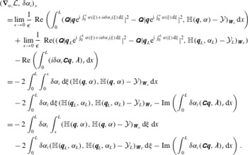 $$\begin{eqnarray}\displaystyle & & \displaystyle (\unicode[STIX]{x1D735}_{\unicode[STIX]{x1D6FC}_{i}}{\mathcal{L}},\unicode[STIX]{x1D6FF}\unicode[STIX]{x1D6FC}_{i})_{x}\nonumber\\ \displaystyle & & \displaystyle \quad =\lim _{\unicode[STIX]{x1D716}\rightarrow 0}\frac{1}{\unicode[STIX]{x1D716}}\text{ Re}\left(\int _{0}^{L}(\unicode[STIX]{x1D64C}|\boldsymbol{q}\text{e}^{\text{i}\int _{0}^{x}\unicode[STIX]{x1D6FC}(\unicode[STIX]{x1D709})+i\unicode[STIX]{x1D716}\unicode[STIX]{x1D6FF}\unicode[STIX]{x1D6FC}_{i}(\unicode[STIX]{x1D709})\,\text{d}\unicode[STIX]{x1D709}}|^{2}-\unicode[STIX]{x1D64C}|\boldsymbol{q}\text{e}^{\text{i}\int _{0}^{x}\unicode[STIX]{x1D6FC}(\unicode[STIX]{x1D709})\,\text{d}\unicode[STIX]{x1D709}}|^{2},\mathbb{H}(\boldsymbol{q},\unicode[STIX]{x1D6FC})-{\mathcal{Y}})_{\unicode[STIX]{x1D652}_{o}}\,\text{d}x\right)\nonumber\\ \displaystyle & & \displaystyle \qquad +\,\lim _{\unicode[STIX]{x1D716}\rightarrow 0}\frac{1}{\unicode[STIX]{x1D716}}\text{ Re}((\unicode[STIX]{x1D64C}|\boldsymbol{q}_{L}\text{e}^{\text{i}\int _{0}^{L}\unicode[STIX]{x1D6FC}(\unicode[STIX]{x1D709})+i\unicode[STIX]{x1D716}\unicode[STIX]{x1D6FF}\unicode[STIX]{x1D6FC}_{i}(\unicode[STIX]{x1D709})\,\text{d}\unicode[STIX]{x1D709}}|^{2}-\unicode[STIX]{x1D64C}|\boldsymbol{q}_{L}\text{e}^{\text{i}\int _{0}^{L}\unicode[STIX]{x1D6FC}(\unicode[STIX]{x1D709})\,\text{d}\unicode[STIX]{x1D709}}|^{2},\mathbb{H}(\boldsymbol{q}_{L},\unicode[STIX]{x1D6FC}_{L})-{\mathcal{Y}}_{L})_{\unicode[STIX]{x1D652}_{T}})\nonumber\\ \displaystyle & & \displaystyle \qquad -\,\text{Re}\left(\int _{0}^{L}(i\unicode[STIX]{x1D6FF}\unicode[STIX]{x1D6FC}_{i}\unicode[STIX]{x1D63E}\boldsymbol{q},\unicode[STIX]{x1D740})_{r}\,\text{d}x\right)\nonumber\\ \displaystyle & & \displaystyle \quad =-\,2\int _{0}^{L}\int _{0}^{x}\unicode[STIX]{x1D6FF}\unicode[STIX]{x1D6FC}_{i}\,\text{d}\unicode[STIX]{x1D709}(\mathbb{H}(\boldsymbol{q},\unicode[STIX]{x1D6FC}),\mathbb{H}(\boldsymbol{q},\unicode[STIX]{x1D6FC})-{\mathcal{Y}})_{\unicode[STIX]{x1D652}_{o}}\,\text{d}x\nonumber\\ \displaystyle & & \displaystyle \qquad -\,2\int _{0}^{L}\unicode[STIX]{x1D6FF}\unicode[STIX]{x1D6FC}_{i}\,\text{d}\unicode[STIX]{x1D709}(\mathbb{H}(\boldsymbol{q}_{L},\unicode[STIX]{x1D6FC}_{L}),\mathbb{H}(\boldsymbol{q}_{L},\unicode[STIX]{x1D6FC}_{L})-{\mathcal{Y}}_{L})_{\unicode[STIX]{x1D652}_{T}}-\text{Im}\left(\int _{0}^{L}\unicode[STIX]{x1D6FF}\unicode[STIX]{x1D6FC}_{i}(\unicode[STIX]{x1D63E}\boldsymbol{q},\unicode[STIX]{x1D740})_{r}\,\text{d}x\right)\nonumber\\ \displaystyle & & \displaystyle \quad =-\,2\int _{0}^{L}\unicode[STIX]{x1D6FF}\unicode[STIX]{x1D6FC}_{i}\int _{x}^{L}(\mathbb{H}(\boldsymbol{q},\unicode[STIX]{x1D6FC}),\mathbb{H}(\boldsymbol{q},\unicode[STIX]{x1D6FC})-{\mathcal{Y}})_{\unicode[STIX]{x1D652}_{o}}\,\text{d}\unicode[STIX]{x1D709}\,\text{d}x\nonumber\\ \displaystyle & & \displaystyle \qquad -\,2\int _{0}^{L}\unicode[STIX]{x1D6FF}\unicode[STIX]{x1D6FC}_{i}(\mathbb{H}(\boldsymbol{q}_{L},\unicode[STIX]{x1D6FC}_{L}),\mathbb{H}(\boldsymbol{q}_{L},\unicode[STIX]{x1D6FC}_{L})-{\mathcal{Y}}_{L})_{\unicode[STIX]{x1D652}_{T}}\,\text{d}\unicode[STIX]{x1D709}-\text{Im}\left(\int _{0}^{L}\unicode[STIX]{x1D6FF}\unicode[STIX]{x1D6FC}_{i}(\unicode[STIX]{x1D63E}\boldsymbol{q},\unicode[STIX]{x1D740})_{r}\,\text{d}x\right).\nonumber\\ \displaystyle & & \displaystyle\end{eqnarray}$$
 $$\begin{eqnarray}\displaystyle (\unicode[STIX]{x1D735}_{\unicode[STIX]{x1D6FC}}{\mathcal{L}},\unicode[STIX]{x1D6FF}\unicode[STIX]{x1D6FC})_{x} & = & \displaystyle \text{Re}\left(\int _{0}^{L}\unicode[STIX]{x1D6FF}\unicode[STIX]{x1D6FC}\left(-2\text{i}\int _{x}^{L}(\mathbb{H}(\boldsymbol{q},\unicode[STIX]{x1D6FC}),\mathbb{H}(\unicode[STIX]{x1D6FC})-{\mathcal{Y}})_{\unicode[STIX]{x1D652}_{o}}\,\text{d}\unicode[STIX]{x1D709}\right.\right.\nonumber\\ \displaystyle & & \displaystyle -\,2\text{i}\left.\left.(\mathbb{H}(\boldsymbol{q}_{L},\unicode[STIX]{x1D6FC}_{L}),\mathbb{H}(\unicode[STIX]{x1D6FC}_{L})-{\mathcal{Y}}_{L})_{\unicode[STIX]{x1D652}_{T}}-(\unicode[STIX]{x1D63E}\boldsymbol{q},\unicode[STIX]{x1D740})_{r}\right)\,\text{d}x\right).\end{eqnarray}$$
D.4 Directional derivative in the directions
$\unicode[STIX]{x1D6FF}\boldsymbol{w}$

 $$\begin{eqnarray}\displaystyle (\unicode[STIX]{x1D735}_{\boldsymbol{w}}{\mathcal{L}},\unicode[STIX]{x1D6FF}\boldsymbol{w})_{xr} & = & \displaystyle \text{Re}\left(\int _{0}^{L}(\unicode[STIX]{x1D6FF}\boldsymbol{w},\boldsymbol{w})_{\unicode[STIX]{x1D652}_{w}}\,\text{d}x\right)-\text{Re}\left(\int _{0}^{L}(-\unicode[STIX]{x1D6FF}\boldsymbol{w},\unicode[STIX]{x1D740})_{r}\,\text{d}x\right)\nonumber\\ \displaystyle & = & \displaystyle \text{Re}\left(\int _{0}^{L}(\unicode[STIX]{x1D6FF}\boldsymbol{w},\unicode[STIX]{x1D652}_{w}\boldsymbol{w}+\unicode[STIX]{x1D740})_{r}\,\text{d}x\right).\end{eqnarray}$$
D.5 Directional derivative in the directions
$\unicode[STIX]{x1D6FF}\boldsymbol{\unicode[STIX]{x1D702}}$

 $$\begin{eqnarray}\displaystyle (\unicode[STIX]{x1D735}_{\boldsymbol{\unicode[STIX]{x1D702}}}{\mathcal{L}},\unicode[STIX]{x1D6FF}\boldsymbol{\unicode[STIX]{x1D702}})_{r} & = & \displaystyle \text{Re}((\unicode[STIX]{x1D6FF}\boldsymbol{\unicode[STIX]{x1D702}},\boldsymbol{\unicode[STIX]{x1D702}})_{\unicode[STIX]{x1D652}_{\unicode[STIX]{x1D702}}})-\text{Re}((-\unicode[STIX]{x1D6FF}\boldsymbol{\unicode[STIX]{x1D702}},\unicode[STIX]{x1D743})_{r})\nonumber\\ \displaystyle & = & \displaystyle \text{Re}((\unicode[STIX]{x1D6FF}\boldsymbol{\unicode[STIX]{x1D702}},\unicode[STIX]{x1D652}_{\unicode[STIX]{x1D702}}\boldsymbol{\unicode[STIX]{x1D702}}+\unicode[STIX]{x1D640}^{+}\unicode[STIX]{x1D740}(0,r)+\boldsymbol{q}_{0}\unicode[STIX]{x1D701}^{\ast }(0))_{r}).\end{eqnarray}$$
D.6 Assembling
Enforcing that
 $(\unicode[STIX]{x1D735}_{\boldsymbol{q}}{\mathcal{L}},\unicode[STIX]{x1D6FF}\boldsymbol{q})_{xr}=0$
leads to
 $$\begin{eqnarray}\displaystyle & & \displaystyle -\text{Re}\left(\int _{0}^{L}\left(\unicode[STIX]{x1D6FF}\boldsymbol{q},-\unicode[STIX]{x1D640}^{+}\frac{\unicode[STIX]{x2202}\unicode[STIX]{x1D740}}{\unicode[STIX]{x2202}x}+\left(\unicode[STIX]{x1D63C}+\unicode[STIX]{x1D6FC}\unicode[STIX]{x1D63E}-\frac{\unicode[STIX]{x2202}\unicode[STIX]{x1D640}}{\unicode[STIX]{x2202}x}\right)^{+}\unicode[STIX]{x1D740}+\frac{\unicode[STIX]{x2202}\boldsymbol{q}}{\unicode[STIX]{x2202}x}(\unicode[STIX]{x1D701}-\unicode[STIX]{x1D701}^{\ast })-\boldsymbol{q}\frac{\unicode[STIX]{x2202}\unicode[STIX]{x1D701}^{\ast }}{\unicode[STIX]{x2202}x}\right.\right.\nonumber\\ \displaystyle & & \displaystyle -\,2|\text{e}^{\text{i}\int _{0}^{x}\unicode[STIX]{x1D6FC}(\unicode[STIX]{x1D709})\,\text{d}\unicode[STIX]{x1D709}}|^{2}\left.\left.((\unicode[STIX]{x1D64C}^{\ast }\unicode[STIX]{x1D64C}\unicode[STIX]{x1D63F}_{\bar{\boldsymbol{q}}})^{+}\unicode[STIX]{x1D64C}^{\ast }\unicode[STIX]{x1D652}_{o}(\mathbb{H}(\boldsymbol{q},\unicode[STIX]{x1D6FC})-{\mathcal{Y}}))\right)_{r}\,\text{d}x\right)=0\end{eqnarray}$$
and
 $$\begin{eqnarray}\displaystyle & & \displaystyle -\text{Re}([(\unicode[STIX]{x1D6FF}\boldsymbol{q},\unicode[STIX]{x1D640}^{+}\unicode[STIX]{x1D740})_{r}]_{0}^{L})\nonumber\\ \displaystyle & & \displaystyle +\,\text{Re}((\unicode[STIX]{x1D6FF}\boldsymbol{q}_{L},2|\text{e}^{\text{i}\int _{0}^{L}\unicode[STIX]{x1D6FC}(\unicode[STIX]{x1D709})\,\text{d}\unicode[STIX]{x1D709}}|^{2}((\unicode[STIX]{x1D64C}^{\ast }\unicode[STIX]{x1D64C}\unicode[STIX]{x1D63F}_{\bar{\boldsymbol{q}}})^{+}\unicode[STIX]{x1D64C}^{\ast }\unicode[STIX]{x1D652}_{T}(\mathbb{H}(\boldsymbol{q}_{L},\unicode[STIX]{x1D6FC}_{L})-{\mathcal{Y}}_{L})))_{r})=0.\end{eqnarray}$$
Enforcing that
 $(\unicode[STIX]{x1D735}_{\unicode[STIX]{x1D6FC}}{\mathcal{L}},\unicode[STIX]{x1D6FF}\unicode[STIX]{x1D6FC})_{x}=0$
leads to
 $$\begin{eqnarray}\displaystyle & & \displaystyle \text{Re}\left(\int _{0}^{L}\unicode[STIX]{x1D6FF}\unicode[STIX]{x1D6FC}\left(-2\text{i}\int _{x}^{L}(\mathbb{H}(\boldsymbol{q},\unicode[STIX]{x1D6FC}),\mathbb{H}(\unicode[STIX]{x1D6FC})-{\mathcal{Y}})_{\unicode[STIX]{x1D652}_{o}}\,\text{d}\unicode[STIX]{x1D709}\right.\right.\nonumber\\ \displaystyle & & \displaystyle -\,2\text{i}\left.\left.(\mathbb{H}(\boldsymbol{q}_{L},\unicode[STIX]{x1D6FC}_{L}),\mathbb{H}(\unicode[STIX]{x1D6FC}_{L})-{\mathcal{Y}}_{L})_{\unicode[STIX]{x1D652}_{T}}-(\unicode[STIX]{x1D63E}\boldsymbol{q},\unicode[STIX]{x1D740})_{r}\right)\,\text{d}x\right)=0.\end{eqnarray}$$
If this is true for any
 $\unicode[STIX]{x1D6FF}\boldsymbol{q}$
and
 $\unicode[STIX]{x1D6FF}\unicode[STIX]{x1D6FC}$
, and (D 15) is respected for any
 $\unicode[STIX]{x1D6FF}\boldsymbol{w}$
, then we get the adjoint system (4.12) with
 $$\begin{eqnarray}\displaystyle \left.\begin{array}{@{}c@{}}\displaystyle RHS_{1}=2|\text{e}^{\text{i}\int _{0}^{x}\unicode[STIX]{x1D6FC}(\unicode[STIX]{x1D709})\,\text{d}\unicode[STIX]{x1D709}}|^{2}((\unicode[STIX]{x1D64C}^{\ast }\unicode[STIX]{x1D64C}\unicode[STIX]{x1D63F}_{\bar{\boldsymbol{q}}})^{+}\unicode[STIX]{x1D64C}^{\ast }\unicode[STIX]{x1D652}_{o}(\mathbb{H}(\boldsymbol{q},\unicode[STIX]{x1D6FC})-{\mathcal{Y}})),\\ \displaystyle RHS_{2}=-2\text{i}\int _{x}^{L}(\mathbb{H}(\boldsymbol{q},\unicode[STIX]{x1D6FC}),\mathbb{H}(\boldsymbol{q},\unicode[STIX]{x1D6FC})-{\mathcal{Y}})_{\unicode[STIX]{x1D652}_{o}}\,\text{d}\unicode[STIX]{x1D709}-2\text{i}(\mathbb{H}(\boldsymbol{q}_{L},\unicode[STIX]{x1D6FC}_{L}),\mathbb{H}(\boldsymbol{q}_{L},\unicode[STIX]{x1D6FC}_{L})-{\mathcal{Y}}_{L})_{\unicode[STIX]{x1D652}_{T}},\\ \displaystyle RHS_{3}=2|\text{e}^{\text{i}\int _{0}^{L}\unicode[STIX]{x1D6FC}(\unicode[STIX]{x1D709})\,\text{d}\unicode[STIX]{x1D709}}|^{2}((\unicode[STIX]{x1D64C}^{\ast }\unicode[STIX]{x1D64C}\unicode[STIX]{x1D63F}_{\bar{\boldsymbol{q}}})^{+}\unicode[STIX]{x1D64C}^{\ast }\unicode[STIX]{x1D652}_{T}(\mathbb{H}(\boldsymbol{q}_{L},\unicode[STIX]{x1D6FC}_{L})-{\mathcal{Y}}_{L})),\end{array}\right\} & & \displaystyle \nonumber\\ \displaystyle & & \displaystyle\end{eqnarray}$$
with
 $\unicode[STIX]{x1D63F}_{\bar{\boldsymbol{q}}}=\text{diag}(\bar{\boldsymbol{q}})$
.
The real parts of the axial components
 $\unicode[STIX]{x1D6FF}\widetilde{\boldsymbol{f}}_{\unicode[STIX]{x1D714},m}$
(isocontours) and
 $\unicode[STIX]{x1D6FF}\widetilde{\boldsymbol{q}}_{\unicode[STIX]{x1D714},m}$
(colourmap) for various Strouhal numbers. Isocontours of the forcing
 $\text{Re}(\unicode[STIX]{x1D6FF}\widetilde{\boldsymbol{f}}_{\unicode[STIX]{x1D714},m}^{u})$
are plotted as solid lines for positive values and dashed lines for negative values.

Finally, if the same procedure is performed using the standard sensitivity observation operator (4.8) instead of (4.9), we obtain the same optimality system, except for
 $$\begin{eqnarray}\displaystyle \left.\begin{array}{@{}c@{}}\displaystyle RHS_{1}=|\text{e}^{\text{i}\int _{0}^{x}\unicode[STIX]{x1D6FC}(\unicode[STIX]{x1D709})\,\text{d}\unicode[STIX]{x1D709}}|^{2}\unicode[STIX]{x1D652}_{o}\boldsymbol{q},\\ \displaystyle RHS_{2}=-\text{i}\int _{x}^{L}\Vert \boldsymbol{q}\text{e}^{\text{i}\int _{0}^{x}\unicode[STIX]{x1D6FC}(\unicode[STIX]{x1D709})\,\text{d}\unicode[STIX]{x1D709}}\Vert _{\unicode[STIX]{x1D652}_{o}}^{2}\,\text{d}\unicode[STIX]{x1D709}-\text{i}\Vert \boldsymbol{q}\text{e}^{\text{i}\int _{0}^{L}\unicode[STIX]{x1D6FC}(\unicode[STIX]{x1D709})\,\text{d}\unicode[STIX]{x1D709}}\Vert _{\unicode[STIX]{x1D652}_{T}}^{2},\\ \displaystyle RHS_{3}=|\text{e}^{\text{i}\int _{0}^{L}\unicode[STIX]{x1D6FC}(\unicode[STIX]{x1D709})\,\text{d}\unicode[STIX]{x1D709}}|^{2}\unicode[STIX]{x1D652}_{T}\boldsymbol{q}.\end{array}\right\} & & \displaystyle\end{eqnarray}$$
D.7 Adjoint of a cumulative integral
In this section, the adjoint of a cumulative integral is detailed. Consider the following term:
 $$\begin{eqnarray}\displaystyle \left(\int _{0}^{x}\unicode[STIX]{x1D6FC}(\unicode[STIX]{x1D709})\,\text{d}\unicode[STIX]{x1D709},y\right)_{x}=\int _{0}^{L}\int _{0}^{x}\unicode[STIX]{x1D6FC}(\unicode[STIX]{x1D709})\,\text{d}\unicode[STIX]{x1D709}y(x)\,\text{d}x. & & \displaystyle\end{eqnarray}$$
We define
 $\unicode[STIX]{x1D6FD}(x)=\int _{0}^{x}\unicode[STIX]{x1D6FC}(\unicode[STIX]{x1D709})\,\text{d}\unicode[STIX]{x1D709}$
such that
 $\text{d}\unicode[STIX]{x1D6FD}/\text{d}x(x)=\unicode[STIX]{x1D6FC}(x)$
, and
 $\unicode[STIX]{x1D6FE}(x)=\int _{L}^{x}y(\unicode[STIX]{x1D709})\,\text{d}\unicode[STIX]{x1D709}$
such that
 $\text{d}\unicode[STIX]{x1D6FE}/\text{d}x(x)=y(x)$
. We have then
 $$\begin{eqnarray}\displaystyle \left(\int _{0}^{x}\unicode[STIX]{x1D6FC}(\unicode[STIX]{x1D709})\,\text{d}\unicode[STIX]{x1D709},y\right)_{x} & = & \displaystyle \int _{0}^{L}\unicode[STIX]{x1D6FD}(x)\frac{\text{d}\unicode[STIX]{x1D6FE}}{\text{d}x}(x)\,\text{d}x\nonumber\\ \displaystyle & = & \displaystyle [\unicode[STIX]{x1D6FD}(x)\unicode[STIX]{x1D6FE}(x)]_{0}^{L}-\int _{0}^{L}\frac{\text{d}\unicode[STIX]{x1D6FD}}{\text{d}x}(x)\unicode[STIX]{x1D6FE}(x)\,\text{d}x\nonumber\\ \displaystyle & = & \displaystyle \left[\int _{0}^{x}\unicode[STIX]{x1D6FC}(\unicode[STIX]{x1D709})\,\text{d}\unicode[STIX]{x1D709}\int _{L}^{x}y(\unicode[STIX]{x1D709})\,\text{d}\unicode[STIX]{x1D709}\right]_{0}^{L}-\int _{0}^{L}\unicode[STIX]{x1D6FC}(x)\int _{L}^{x}y(\unicode[STIX]{x1D709})\,\text{d}\unicode[STIX]{x1D709}\,\text{d}x\nonumber\\ \displaystyle & = & \displaystyle \left(\unicode[STIX]{x1D6FC}(x),\int _{x}^{L}y(\unicode[STIX]{x1D709})\,\text{d}\unicode[STIX]{x1D709}\right)_{x}.\end{eqnarray}$$
The real parts of the axial components
 $\unicode[STIX]{x1D6FF}\widetilde{\boldsymbol{f}}_{\unicode[STIX]{x1D714},m}$
(isocontours) and
 $\unicode[STIX]{x1D6FF}\widetilde{\boldsymbol{q}}_{\unicode[STIX]{x1D714},m}$
(colourmap) for various Strouhal numbers. Isocontours of the forcing
 $\text{Re}(\unicode[STIX]{x1D6FF}\widetilde{\boldsymbol{f}}_{\unicode[STIX]{x1D714},m}^{u})$
are plotted as solid lines for positive values and dashed lines for negative values.

Centreline streamwise fluctuating energy: first POD mode of PIV measurements (○), observation operator for homogeneous PSE (


Converged 4D-Var: real parts of the axial components
 $\widetilde{\boldsymbol{f}}_{\unicode[STIX]{x1D714},m}$
(isocontours) and
 $\unicode[STIX]{x1D6FF}\widetilde{\boldsymbol{q}}_{\unicode[STIX]{x1D714},m}$
(colourmap) for various Strouhal numbers. Isocontours of the forcing
 $\text{Re}(\unicode[STIX]{x1D6FF}\widetilde{\boldsymbol{f}}_{\unicode[STIX]{x1D714},m}^{u})$
plotted as solid lines for positive values and dashed lines for negative values.

Appendix E. Sensitivity of PSE-4D-Var for various Strouhal numbers
In this appendix, we show the behaviour of the sensitivity of a wavepacket to forcing for various Strouhal numbers. Figures 23 and 24 show
 $\text{Re}(\unicode[STIX]{x1D6FF}\widetilde{\boldsymbol{f}}_{\unicode[STIX]{x1D714},m}^{u})$
and the associated response
 $\text{Re}(\unicode[STIX]{x1D6FF}\widetilde{\boldsymbol{q}}_{\unicode[STIX]{x1D714},m}^{u})$
. The behaviour is qualitatively the same in the frequency range between
 $St=0.3$
and
 $St=0.7$
, with a contraction in space as the Strouhal number increases. For
 $St<0.3$
, mismatches between wavepacket models and experiments remain misunderstood (see figure 1), and were not investigated here. High Strouhal numbers are limited here by aliasing effects of experimental measurements of
 ${\mathcal{Y}}$
(Cavalieri et al.
Reference Cavalieri, Rodriguez, Jordan, Colonius and Gervais2013) used in 4D-Var.
Appendix F. Converged PSE-4D-Var results for various Strouhal numbers
We display here results of the converged 4D-Var for various Strouhal numbers in order to show that the trend discussed in § 4.2.3 is preserved. Figure 25 displays centreline values of the streamwise component of measurements, homogeneous PSE and PSE forced by 4D-Var. For all Strouhal numbers, the forcing is able to make the PSE follow the reference experimental results accurately.
Figure 26 plots the forcing and response of the converged 4D-Var. The trend detailed in § 4.2.3 is also preserved.