1. Introduction
1.1 Overview
The purpose of this paper is to establish a version of Seiberg–Witten Floer K-theory for knots that is derived from a version of Seiberg–Witten Floer K-theory for 3-manifolds with involutions through double branched covers. Our construction is based on Manolescu’s Seiberg–Witten Floer stable homotopy type [Reference ManolescuMan03] and an involutive symmetry on the Seiberg–Witten equations introduced by Kato [Reference KatoKat22]. Kato’s involution on the Seiberg–Witten equations takes the effects of given involutions on 4-manifolds into account, but his framework is not an equivariant Seiberg–Witten theory in the usual sense. (See § 1.7 for details.) While Kato [Reference KatoKat22] considered closed spin 4-manifolds, in this paper we develop a three-dimensional version of [Reference KatoKat22] and extend Kato’s work to 4-manifolds with boundary.
While various researchers have studied the effects of group actions in several types of Floer homology and their applications to knots, e.g. [Reference HendricksHen12, Reference Karakurt and LidmanKL15, Reference Hendricks, Lipshitz and SarkarHLS16, Reference Hendricks and ManolescuHM17, Reference Lidman and ManolescuLM18, Reference Lin, Ruberman and SavelievLRS18, Reference KangKan18b, Reference KangKan18a, Reference Hendricks and LipshitzHL19, Reference LargeLar19, Reference Hendricks, Lipshitz and SarkarHLS20a, Reference Alfieri, Kang and StipsiczAKS20, Reference Lin, Ruberman and SavelievLRS22, Reference Hendricks, Lipshitz and SarkarHLS20b, Reference Hendricks, Lidman and LipshitzHLL22, Reference Dai, Hedden and MallickDHM22, Reference Baraglia and HekmatiBH24, Reference Collin and SteerCS99, Reference Kronheimer and MrowkaKM11, Reference Daemi and ScadutoDS24], to the best of our knowledge, this paper is the first study of Floer K-theory defined for knots with a 10/8-type inequality. Like the original 10/8-inequality by Furuta [Reference FurutaFur01] and its generalization to 4-manifolds with boundary by Manolescu [Reference ManolescuMan14], constraints on knots obtained from our 10/8-type inequality are much different from constraints obtained from usual (i.e. ordinary cohomological) Floer theory for 3-manifolds with involutions. More concretely, our framework has the advantage that it yields a constraint on the intersection forms of indefinite 4-manifolds. Moreover, the constraint is significantly different from [Reference FurutaFur01, Reference ManolescuMan14] as an effect of the existence of involutions, which shall be explained in Remark 1.3.
Our main results are 10/8-type inequalities for spin 4-manifolds with boundary and with involution, and for surfaces bounded by knots. The 10/8-inequality for knots yields numerous interesting applications to bounds on stabilizing numbers and relative genera. Representative applications to knots from our framework shall be described in Theorems 1.13 and 1.14. Theorem 1.13 detects a difference between the topological category and the smooth category from a new point of view: a comparison between topological and smooth stabilizing numbers. Theorem 1.14 shows that there is a discrepancy between topological and smooth minimal genera for knots embedded into the boundary of a punctured 4-manifold. These applications shall be derived from a Floer K-theoretic knot concordance invariant we shall define. At first glance it is difficult to calculate this invariant because we use analytic information from the Seiberg–Witten equations to define the invariant. However, we can calculate this invariant for some class of knots: 2-bridge knots (Theorem 1.8), torus knots (Theorem 1.9), and their linear combinations (Theorem 1.10). Our 10/8-type inequality also obstructs extending involutions on 3-manifolds to spin 4-manifolds, as stated in Theorem 1.16. This obstruction is strong enough to detect non-smoothable group actions: this is summarized in Theorem 5.6.
We hope that, in future work, ideas in this paper will be developed further; for example, defining an invariant of surface knots and giving a lower bound on unoritable genera of knots as next steps.
1.2 Relative 10/8-inequality for involutions
Let Y be an oriented rational homology 3-sphere,
 $\mathfrak{t}$
be a spin structure on Y, and
 $\iota$
be an orientation-preserving smooth involution whose fixed-point set is non-empty and of codimension-2. Suppose that
 $\iota$
preserves the spin structure
 $\mathfrak{t}$
. (If Y is a
 $\mathbb{Z}_2$
-homology 3-sphere, this is the case for all
 $\iota$
.) We shall define a numerical invariant
 \[\kappa(Y, \mathfrak{t}, \iota) \in \tfrac{1}{16}\mathbb{Z} \]
of a
 $\mathbb{Z}/2\mathbb{Z}$
-equivariant diffeomorphism class of a triple
 $(Y, \mathfrak{t}, \iota)$
. We call this invariant
 $\kappa(Y, \mathfrak{t}, \iota)$
the K-theoretic Frøyshov invariant of the triple
 $(Y, \mathfrak{t}, \iota)$
. This is a version (taking the effects of
 $\iota$
into account) of the K-theoretic invariant
 $\kappa(Y,\mathfrak{t})$
introduced by Manolescu [Reference ManolescuMan14], which was used in [Reference ManolescuMan14] to establish a relative version of Furuta’s 10/8-inequality [Reference FurutaFur01].
Most of the results of this paper follow from a relative 10/8-type inequality for spin 4-manifolds with involution as described below. For triples
 $(Y_0, \mathfrak{t}_0,\iota_0)$
and
 $(Y_1, \mathfrak{t}_1,\iota_1)$
, we call a triple
 $(W,\mathfrak{s},\iota)$
a smooth spin cobordism with involution from
 $(Y_0, \mathfrak{t}_0,\iota_0)$
to
 $(Y_1, \mathfrak{t}_1,\iota_1)$
if
 $(W,\mathfrak{s})$
is a smooth compact connected oriented spin cobordism from
 $(Y_0, \mathfrak{t}_0)$
to
 $(Y_1, \mathfrak{t}_1)$
and
 $\iota$
is a smooth involution of W which preserves the orientation and the spin structure
 $\mathfrak{s}$
and whose restriction to the boundary is given by
 $\iota_0 \sqcup \iota_1$
. Let
 $b^+_\iota(W)$
denote the maximal dimension of
 $\iota$
-invariant positive-definite subspaces of
 $H^2(W;\mathbb{R})$
. The focus of the following theorem is property (iv), which is our relative 10/8-inequality for involutions.
Theorem 1.1. Let
 $(Y, \mathfrak{t})$
be an oriented spin rational homology 3-sphere and
 $\iota$
be an orientation-preserving smooth involution on Y whose fixed-point set is non-empty and of codimension-2 and which preserves the spin structure
 $\mathfrak{t}$
. We can associate an invariant
 $\kappa(Y, \mathfrak{t}, \iota) \in \frac{1}{16}\mathbb{Z}$
to every such triple
 $(Y, \mathfrak{t}, \iota)$
with the following properties.
-
(i) The mod 2 reduction of
 $-2\kappa(Y, \mathfrak{t}, \iota)$
coincides with the Rokhlin invariant
$\mu(Y,\mathfrak{t})$
:
\[-2 \kappa (Y, \mathfrak{t}, \iota) = \mu (Y , \mathfrak{t}) \text{ in } ( \tfrac{1}{8} \mathbb{Z} ) / 2\mathbb{Z} \cong \mathbb{Z}/16\mathbb{Z}. \]
-
(ii) The quantity
$\kappa (Y, \mathfrak{t}, \iota)$
is invariant under conjugation: for every diffeomorphism f on Y preserving the orientation and the spin structure
$\mathfrak{t}$
, we have
\[\kappa (Y, \mathfrak{t}, \iota) = \kappa (Y, \mathfrak{t}, f^{-1} \circ \iota \circ f). \]
-
(iii) For
$-Y$
, the same manifold with the reversed orientation, we have
\[\kappa(Y,\mathfrak{t},\iota) + \kappa(-Y,\mathfrak{t},\iota)\geqslant 0. \]
-
(iv) Let
$(W,\mathfrak{s},\iota)$
be a smooth spin cobordism with involution from
$(Y_0, \mathfrak{t}_0,\iota_0)$
to
$(Y_1, \mathfrak{t}_1,\iota_1)$
with
$b_1(W)=0$
. Then we have


 \begin{align}-\frac{\sigma(W)}{16} + \kappa (Y_0, \mathfrak{t}_0, \iota_0 )\leqslant b^+(W)-b^+_{\iota}(W) + \kappa (Y_1, \mathfrak{t}_1, \iota_1 ).\end{align}
Remark 1.2. If
 $Y=S^3$
, regarded as a subset of
 $\mathbb{C}^2$
, and
 $\iota : Y\to Y$
is the complex conjugation, we shall see in Example 3.46 that
 $\kappa(Y,\mathfrak{t},\iota)=0$
for the unique spin structure
 $\mathfrak{t}$
on
 $S^3$
. Thus we can deduce from (1.1) a similar statement for a one-boundary component spin 4-manifold with involution. Also, taking
 $Y_0=Y_1=S^3$
with complex conjugation, Theorem 1.1 recovers Kato’s 10/8-inequality [Reference KatoKat22, Theorem 2.3] for closed spin 4-manifolds.
Remark 1.3. A notable point in the inequality (1.1) is that, in the right-hand side,
 $b^+(W)-b^+_{\iota}(W)$
appears rather than
 $b^+(W)$
as in Furuta’s 10/8-inequality or Manolescu’s relative 10/8-inequality. It shall turn out that this difference is crucial in our applications to knots.
Moreover, we can generalize Theorem 1.1 to fixed-point free odd involutions. See Theorems 3.29 and 3.30.
1.3 K-theoretic knot concordance invariant
Applying Floer theory with involutive symmetry to the double branched covers, several knot (concordance) invariants are defined in Heegaard Floer homology [Reference HendricksHen12, Reference Karakurt and LidmanKL15, Reference Hendricks, Lipshitz and SarkarHLS16, Reference Hendricks, Lidman and LipshitzHLL22, Reference Hendricks, Lipshitz and SarkarHLS20a, Reference Alfieri, Kang and StipsiczAKS20, Reference Dai, Hedden and MallickDHM22] and Seiberg–Witten Floer theory [Reference Baraglia and HekmatiBH24]. Via orbifold gauge theory, several versions of knot instanton Floer homology are developed [Reference Collin and SteerCS99, Reference Kronheimer and MrowkaKM11, Reference Daemi and ScadutoDS24]. We also provide a knot concordance invariant from our Floer K-theory for 3-manifolds with involution.
For simplicity, we consider oriented knots throughout the paper, while our invariant of knots itself is independent of the choice of orientation. For a given knot K in
 $S^3$
, one can associate an oriented rational homology 3-sphere
 $\Sigma(K)$
called the branched covering space along K, which is equipped with the covering involution
 $\iota_K$
. Define the K-theoretic Frøyshov invariant for the knot K by
 \[\kappa (K) := \kappa (\Sigma(K) , \mathfrak{t}, \iota_K) \in \tfrac{1}{16}\mathbb{Z}, \]
where
 $\mathfrak{t}$
is a spin structure on
 $\Sigma(K)$
, which is unique since it is known that
 $H^1(\Sigma(K);\mathbb{Z}/2)=0$
. As a consequence of Theorem 1.1, we prove the following properties of
 $\kappa(K)$
, which includes a 10/8-type inequality for knots: the property (v) below.
Theorem 1.4. The invariant
 $\kappa (K)$
satisfies the following properties.
-
(i) The invariant
$\kappa (K)$
is a knot concordance invariant with
$\kappa(U)=0$
, where U is the unknot. -
(ii) For every knot K, we have
$\kappa (K) = \kappa (-K)$
, where
$-K$
is the knot with the opposite orientation. -
(iii) For every knot K in
$S^3$
, we have
\[2 \kappa (K) =- \tfrac{1}{8} \sigma (K) \text{ in } ( \tfrac{1}{8} \mathbb{Z} ) / 2\mathbb{Z} \cong \mathbb{Z}/16\mathbb{Z}. \]
-
(iv) For every knot K in
$S^3$
, we have
$\kappa (K) + \kappa (K^* ) \geqslant 0$
, where
$K^*$
denotes the mirror image of K. -
(v) Let K and K’ be knots in
$S^3$
, X be an oriented smooth compact connected cobordism from
$S^3$
to
$S^3$
with
$H_1(X; \mathbb{Z})=0$
, and S be an oriented compact connected properly and smoothly embedded cobordism in X from K to K’ such that the homology class [S] of S is divisible by 2 and
$PD(w_2(X)) = [S]/2 \operatorname{mod} 2$
. Then we have(1.2)
\begin{align} -\frac{\sigma(X)}{8} + \frac{9}{32}[S]^2-\frac{9}{16}\sigma(K') + \frac{9}{16}\sigma(K) \leqslant b^+(X) + g(S) + \kappa(K')-\kappa(K), \end{align}
where
$\sigma(K)$
denotes the signature of K (with the sign convention
$\sigma(T(2,3))=-2$
) and g(S) is the genus of S.


Remark 1.5. If X is spin, K, K’ are the unknots, and S is a null-homologous smoothly embedded annulus, then the inequality (1.2) implies
 $-\sigma(X)/8 \leqslant b^+(X)$
, which recovers Furuta’s original 10/8-inequality [Reference FurutaFur01] except for adding 1 on the left-hand side. Note that one can deduce a constraint on surfaces bounded by knots from Manolescu’s relative 10/8-inequality [Reference ManolescuMan14] applied to the branched covering spaces. In Appendix A, we shall summarize such constraints following from known results. Also, the invariant
 $\kappa$
can be extended to an invariant of a pair (Y, K) of an oriented homology 3-sphere Y and a knot K in Y. For more details, see Remark 3.55.
Remark 1.6. It could be interesting to consider an approach to the 11/8-conjecture due to Matsumoto [Reference MatsumotoMat82] from Theorem 1.4. In short, if one can find a suitable embedded surface S in a spin 4-manifold X, one can refine the 10/8-inequality for X. See Corollary 4.5.
We record a genus bound on closed surfaces in a closed 4-manifold deduced from Theorem 1.4.
Corollary 1.7. Let X be a closed oriented smooth 4-manifold with
 $H_1(X ;\mathbb{Z}) =0 $
, and let S be an oriented compact properly smoothly embedded surface S in X such that the homology class [S] of S is divisible by 2 and
 $PD(w_2(X)) = [S]/2 \operatorname{mod} 2$
. Then we have
 \[-\frac{\sigma(X)}{8} + \frac{9}{32}[S]^2 \leqslant b^+(X) + g(S). \]
Proof. Setting
 $K= K ' = U$
, the unknot, the inequality (1.2) gives the claim.
As another genus bound for closed 4-manifolds obtained via double branched coverings, see also [Reference Kotschick and MatićKM95, Theorem 3.1], where the authors applied Donaldson’s theorems A, B and C to double branched coverings.
Next, we shall exhibit calculations of
 $\kappa(K)$
for 2-bridge knots.
Theorem 1.8. For coprime integers p, q with p odd, let K(p, q) be the two bridge knot of type (p, q) whose branched cover is the lens space L(p, q). Then we have
 \begin{align}\kappa (K(p,q)) = -\tfrac{1}{16} \sigma (K(p,q)).\end{align}
Equation (1.3) also holds for every connected sum of two bridge knots.
More interestingly, we can also compute
 $\kappa(K)$
for many torus knots. This is a consequence of the fact that our Seiberg–Witten Floer stable homotopy types for torus knots turn out to be sphere spectra, which correspond to the simplest type of Floer homology. This makes a striking contrast to known knot Floer homology theories, since they tend to have more complicated Floer homology for torus knots.
Theorem 1.9. Let p,q be coprime odd integers and T(p,q) be the torus knot of type (p,q). Then the equality
 \[\kappa ( T(p,q) ) = - \tfrac{1}{2} \bar{\mu} (\Sigma (2,p,q) ) \]
holds, where
 $\bar{\mu}$
is the Neumann–Siebenmann invariant. Moreover, the equality
 $\kappa (K) =- \frac{1}{2}\bar{\mu} (\Sigma (K))$
holds for every connected sum of torus knots T(p,q) for coprime odd integers p and q.
To further compute
 $\kappa (K)$
, we provide the following connected sum formula.
Theorem 1.10. Let K be a knot in
 $S^3$
and K’ be a connected sum of knots appearing in Theorems 1.8 and 1.9. Then we have
 \[ \kappa (K \# K') = \kappa (K) + \kappa (K') . \]
We also give a crossing change formula of
 $\kappa$
using Theorem 1.4.
Theorem 1.11. Let K and K’ be knots in
 $S^3$
.
-
(i) Suppose K’ is obtained from K by a sequence of n-crossing changes. Then the inequality
holds.
\[|\kappa (K')- \kappa (K) + \tfrac{9}{16}\sigma (K') - \tfrac{9}{16}\sigma (K) | \leqslant n \]
-
(ii) Suppose K’ is obtained from K by a sequence of positive crossing changes. Then the inequality
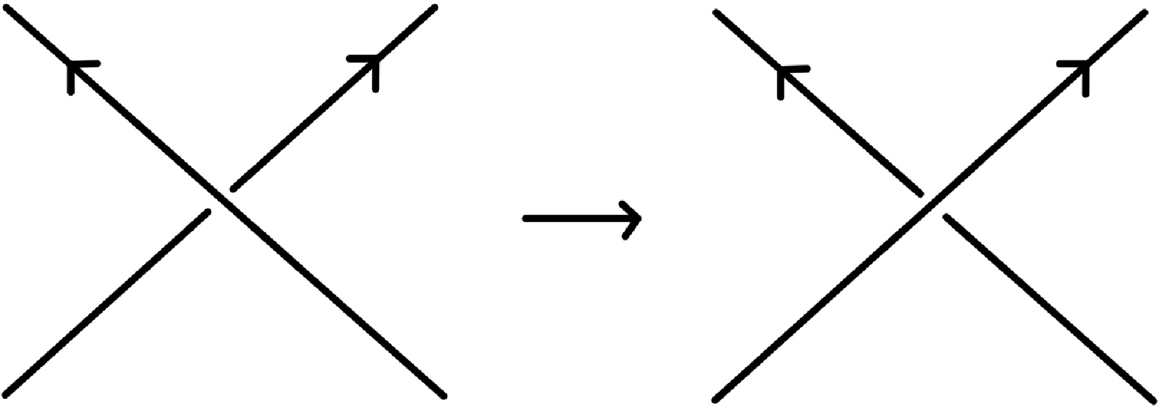
holds, where our convention on the positive crossing change is described in Figure 1.
\[ \kappa (K')- \kappa (K) \leqslant - \tfrac{9}{16}\sigma (K') + \tfrac{9}{16}\sigma(K) \]
Figure 1.Positive crossing change.


It is not difficult to prove a similar full-twist formula under a certain assumption. See Remark 4.6. In Appendix B, we give calculations of
 $\kappa (K)$
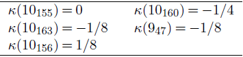
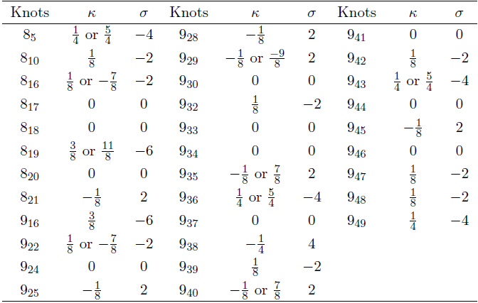
for prime knots with 8- or 9-crossings using Theorem 1.11 combined with Theorem 1.4 (iii). The result is summarized in Theorem 4.7.
1.4 Applications to stabilizing numbers
The results explained in § 1.3 have various applications to four-dimensional aspects of knot theory. We exhibit some of representative applications in this introduction. The first one is to detect the difference of topological and smooth stabilizing numbers. A given knot K in
 $S^3$
is said to be smoothly (respectively topologically) H-slice in X if there exists a proper and smooth (respectively locally flat) null-homologus embedding of a two-dimensional disk bounded by K in
 $X \setminus \operatorname{int}D^4$
. It is proven in [Reference KauffmanKau87, p. 84, Corollary 5.11] and [Reference SchneidermanSch10] that, for every knot K in
 $S^3$
whose Arf invariant
 $\operatorname{Arf}(K)$
is zero, there is a positive integer N such that K is smoothly H-slice in
 $\#_N S^2\times S^2$
, the N-fold connected sum of copies of
 $S^2 \times S^2$
. This result enables us to define invariants

and

when
 $\operatorname{Arf}(K)$
is zero. These quantities have been studied in the literature, and for example in [Reference Conway and NagelCN20], the invariant
 $\operatorname{sn}(K)$
(respectively
 $\operatorname{sn}^{\mathrm{Top}}(K)$
) is called the smooth (respectively topological) stabilizing number of K.
Our invariant
 $\kappa (K)$
can be used to give a lower bound on
 $\operatorname{sn}(K)$
.
Theorem 1.12. For every knot K in
 $S^3$
with
 $\operatorname{Arf}(K) =0$
, we have
 \[ -\tfrac{9 }{16} \sigma (K) - \kappa (K) \leqslant \operatorname{sn}(K). \]
It is a natural and basic question whether the topological stabilizing number and smooth stabilizing number have an essential difference. More concretely, it is asked in [Reference Conway and NagelCN20, Question 1.4] whether there exists a knot K such that
 \[ 0 \lt \operatorname{sn}^{\mathrm{Top}}(K) \lt \operatorname{sn}(K). \]
We give an affirmative answer to this question, and more.
Theorem 1.13. There exists a knot K in
 $S^3$
with
 $\operatorname{Arf}(K) = 0$
that satisfies the following properties.
-
– We have
 \[ 0 \lt \operatorname{sn}^{\mathrm{Top}}(K) \lt \operatorname{sn}(K). \]
-
– We have
$0<\operatorname{sn}(\#_n K )$
for all positive integers n, and
\[ \lim_{n\to \infty }( \operatorname{sn}(\#_n K )- \operatorname{sn}^{\mathrm{Top}}(\#_n K) ) = \infty. \]


For example, we can take K in Theorem 1.13 to be T(3, 11). Moreover, in fact, we may detect many examples of K that satisfy the statement of Theorem 1.13. See Theorem 4.13 for more examples.
To the best of the authors’ knowledge, Theorem 1.13 cannot be derived from any known method, including a constraint from Manolescu’s relative 10/8-inequality summarized in Theorem A.1.
1.5 Applications to relative genera
One of the most classical problems in low-dimensional topology is the study of genus bounds of embedded surfaces in 4-manifolds. For a given knot in
 $S^3$
, one may consider bounds on genera of surfaces bounded by the knot in a punctured 4-manifold. We shall apply the results explained in § 1.3 to this problem.
Let X be an oriented smooth closed 4-manifold with a second homology class
 $x \in H_2(X;\mathbb{Z})$
. For a knot K in
 $S^3$
, let
 $g_{X,x}(K)$
be the minimum of genera of surfaces S that are properly and smoothly embedded oriented connected compact surfaces in
 $X \setminus \operatorname{int} D^4$
such that
 $\partial S =K$
and
 $[S] =x \in H_2(X;\mathbb{Z})$
. Here, [S] denotes the relative fundamental class of S, and
 $H_2(X;\mathbb{Z})$
is naturally identified with
 $H_2(X \setminus \operatorname{int} D^4;\mathbb{Z})$
. This quantity
 $g_{X,x}(K)$
is called the smooth (X,x)-genus of K, and the topological version
 $g^{\mathrm{Top}}_{X,x}(K)$
is defined by considering locally flat embeddings instead of smooth embeddings. The genera
 $g^{\mathrm{Top}}_{X,x}(K)$
and
 $g_{X,x}(K)$
are natural generalizations of classical invariants: the topological and smooth 4-genera (or slice genera), which are defined as
 $g^{\mathrm{Top}}_{S^4,0}(K)$
and
 $g_{S^4,0}(K)$
. There are various known lower bounds on
 $g^{\mathrm{Top}}_{X,x}(K)$
, such as those in [Reference GilmerGil81, Reference Manolescu, Marengon and PiccirilloMMP20, Reference RobertelloRob65, Reference Freedman and KirbyFK78, Reference Klug and RuppikKR21, Reference Conway and NagelCN20]. There are also known lower bounds on
 $g_{X,x}(K)$
for both definite 4-manifolds (for examples, see [Reference Ozsváth and SzabóOS03, Reference Kronheimer and MrowkaKM13, Reference Manolescu, Marengon, Sarkar and WillisMMSW23]) and indefinite 4-manifolds [Reference Mrowka and RollinMR06, Reference Hedden and RaouxHR23, Reference Iida, Mukherjee and TaniguchiIMT21]. However, for indefinite 4-manifolds with vanishing gauge-theoretic invariant, there are few ways to obtain lower bounds on
 $g_{X,x}(K)$
, except for an approach based on 10/8-inequality [Reference Manolescu, Marengon and PiccirilloMMP20].
There is a big difference between the topological and smooth 4-genera: it follows from the affirmative answer to the Milnor conjecture by Kronheimer and Mrowka [Reference Kronheimer and MrowkaKM93] and a recent result by Baader, Banfield and Lewark [Reference Baader, Banfield and LewarkBBL20] on topological slice genus that
 \[\lim_{n\to \infty} (g_{S^4,0}(K_n ) - g^{\mathrm{Top}}_{S^4,0}( K_n )) = \infty \]
for
 $K_n=T(3,12n-1)$
, the torus knot of type
 $(3,12n-1)$
. A similar observation can be applied to definite 4-manifolds X and to every
 $x \in H_2(X;\mathbb{Z})$
using the Ozváth–Szabó
 $\tau$
-invariant [Reference Ozsváth and SzabóOS03], and one obtains
 $\lim_{n\to \infty} (g_{X,x}(K_n ) - g^{\mathrm{Top}}_{X,x}(K_n )) = \infty$
.
We prove that, for every smooth closed 4-manifold X with vanishing first homology, there is a big difference between
 $g_{X,x}(K)$
and
 $g^{\mathrm{Top}}_{X,x}(K)$
.
Theorem 1.14. There exists a knot K’ that satisfies the following property. Let X be a smooth closed oriented 4-manifold with
 $H_1(X;\mathbb{Z}) =0$
, and let
 $x \in H_2(X;\mathbb{Z})$
be a second homology class which is divisible by 2 and satisfies
 $x/2 = PD(w_2(X)) \operatorname{mod} 2$
. Then, for every knot K in
 $ S^3$
, we have
 \[ \lim_{n\to \infty} (g_{X,x}( K \# (\#_n K') ) - g^{\mathrm{Top}}_{X,x}(K \# (\#_n K') ) ) = \infty. \]
Concretely, we can take K’ in Theorem 1.14 to be, for example,
 $K'=T(3,11)$
. A remarkable feature of Theorem 1.14 is that we do not have to impose any restriction on the intersection form of X.
Remark 1.15. The existence of a family of knots
 $\{K_n\}_{n\in \mathbb{Z}_{>0}} $
satisfying
 \[\lim_{n\to \infty} (g_{X,x}(K_n ) - g^{\mathrm{Top}}_{X,x}(K_n )) = \infty \]
under the same assumption on (X, x) in Theorem 1.14 also follows from a constraint obtained from Manolescu’s relative 10/8-inequality [Reference ManolescuMan14] summarized in Theorem A.1. Indeed, one can take
 $K_n=T(3,12n+1)$
for
 $n \geqslant 1$
.
In § 4.2, we give several lower bounds on relative genera stronger than known ones for a class of 4-manifolds including
 $\#_n K3$
and
 $\#_n\mathbb{C} P^2\#_m\overline{\mathbb{C} P}^2$
, summarized in Theorems 4.18 and 4.20, respectively.
1.6 Applications to non-extendable and non-smoothable actions
In § 5, we use Theorem 1.1 to obstruct an extension of involutions on 3-manifolds to spin 4-manifolds. Regard Brieskorn homology spheres
 $\Sigma(p,q,r)$
as a subset of
 $\mathbb{C}^3$
following the standard definition. Consider the involution
 $\iota$
on
 $\Sigma(2,q,r)$
defined by
 $\iota(z_1,z_2,z_3)=(-z_1,z_2,z_3)$
. A recent result by Anvari and Hambleton [Reference Anvari and HambletonAH21, Theorem A] showed that the standard finite cyclic group actions on
 $\Sigma(p,q,r)$
does not extend to any contractible smooth 4-manifold bounded by
 $\Sigma(p,q,r)$
(if it exists) as a smooth involution. In particular,
 $\iota$
does not extend to any contractible smooth 4-manifold bounded by
 $\Sigma(2,q,r)$
as a smooth involution. (See also recent work by Baraglia and Hekmati [Reference Baraglia and HekmatiBH24, Example 7.7].) As a complementary result, we prove the obstruction to extending such
 $\iota$
to non-contractible 4-manifolds for some class of Brieskorn homology spheres.
Theorem 1.16. Let
 $a_{1}, \ldots, a_{n}$
be pairwise coprime natural numbers. Suppose that
 $a_{1}$
is an even number. Set
 $Y=\Sigma(a_{1}, \ldots, a_{n})$
, and define an involution
 $\iota : Y \to Y$
by
 \[\iota(z_1,z_2, \ldots,z_n)=(-z_1,z_2,\ldots,z_n). \]
For all compact connected smooth oriented spin 4-manifold W bounded by Y with
 $b_1(W)=0$
, we have the following.
-
(i) The involution
$\iota$
does not have an extension to W as a smooth involution satisfying
\begin{align*}-\frac{\sigma(W)}{16}> b^+(W)-b^+_{\iota}(W) - \frac{\bar{\mu}(Y)}{2}.\end{align*}
-
(ii) Suppose that
$\sigma(W) \neq 8\bar{\mu}(Y)$
. Then
$\iota$
cannot extend to W as a homologically trivial smooth involution, while
$\iota$
can extend to W as a homologically trivial diffeomorphism.


It is well known that if a Seifert homology sphere bounds a smooth homology 4-ball, then its Neumann–Siebenmann invariant vanishes. This shows that Theorem 1.16 is complementary to the aforementioned results by Anvari and Hambleton [Reference Anvari and HambletonAH21] and by Baraglia and Hekmati [Reference Baraglia and HekmatiBH24] about contractible or homology ball bounds. The results of Theorem 1.16 shall be extended to connected sums of Seifert homology spheres in Theorem 5.3.
The constraint on smooth involutions given in Theorem 1.16 is strong enough to detect non-smoothable group actions as follows. Let
 $\iota_r : S^2\times S^2 \to S^2\times S^2$
be an orientation-preserving smooth involution defined as the product of the
 $\pi$
-rotation of
 $S^2$
along an axis and the identity of
 $S^2$
. Let M(p,q,r) denote the Milnor fiber associated to the singularity
 $z_1^p+z_2^q+z_3^r=0$
.
Theorem 1.17. Let W be the 4-manifold defined by
 \[W = M(2,3,6n-1)\#_{2n+1} S^2 \times S^2 \]
for
 $n\geqslant 2$
, with boundary
 $\Sigma(2,3,6n-1)$
. Then there exists a locally linear topological involution
 $\iota_W : W \to W$
with non-empty fixed-point set that satisfies the following properties.
-
(I) The involution
$\iota_W$
is not smooth with respect to every smooth structure on W. -
(II) The restriction of
$\iota_W$
to the boundary
$\partial{W}$
is the involution
$\iota : \Sigma(2,3,6n-1) \to \Sigma(2,3,6n-1)$
defined by
$\iota(z_1, z_2, z_3) = (-z_1, z_2, z_3)$
. In particular,
$\iota_W|_{\partial W}$
extends as a diffeomorphism of W for every smooth structure on W. -
(III) For any
$N>1$
, the equivariant connected sum along fixed points is also a non-smoothable involution with respect to every smooth structure on
\[\iota_W \#_N \iota_r : W \#_N S^2 \times S^2 \to W \#_N S^2 \times S^2 \]
$W \#_N S^2 \times S^2$
.
-
(IV) The quotient orbifold
$W/\iota_W$
is indefinite. More precisely,
$b^+(W/\iota_W) = b^-(W/\iota_W) = 4n$
.


Property (III) means that the non-smoothability of
 $\iota_W$
is stable under a suitable equivariant connected sum. Theorem 1.17 shall be generalized in Theorem 5.6 for connected sums of W, and also
 $M(2,3,6n+1)$
shall be treated instead of
 $M(2,3,6n-1)$
.
1.7 Floer homotopy type and Floer K-theory
All the results explained until the previous subsection are derived from Theorem 1.1. The main ingredients to establish Theorem 1.1 are versions of Floer homotopy type and of Floer K-theory. Let us clarify the nature of our construction of these ingredients in this subsection.
Based upon Manolescu’s construction of Seiberg–Witten Floer stable homotopy type [Reference ManolescuMan03], we shall construct versions of Seiberg–Witten Floer stable homotopy type for involutions
 \[\textit{DSWF}_G(Y, \mathfrak{t},\iota) \]
and of Seiberg–Witten Floer K-theory for involutions
 \[\textit{DSWFK}_G(Y, \mathfrak{t},\iota), \]
which are defined for a spin rational homology 3-sphere
 $(Y, \mathfrak{t})$
with an involution
 $\iota$
which preserves
 $\mathfrak{t}$
and whose fixed-point set is of codimension-2. Here G stands for
 $G=\mathbb{Z}_4$
, which is the subgroup of
 $\mathrm{Pin}(2)$
generated by
 $j \in \mathrm{Pin}(2)$
, and D stands for a ‘doubling’ construction that is introduced in § 3.3.
Via double branched covers, we obtain the Seiberg–Witten Floer stable homotopy type of a knot K in
 $S^3$
 \[\textit{DSWF}(K) \]
and the Seiberg–Witten Floer K-theory of a knot K
 \[\textit{DSWFK}(K). \]
These are closely related to recent work by Baraglia and Hekmati [Reference Baraglia and HekmatiBH24], where they established an equivariant Seiberg–Witten Floer stable homotopy type for finite group actions on spin
 $^c$
3-manifolds, and an equivariant Seiberg–Witten Floer cohomology, and defined knot invariants in a similar way. (Note also a recent combinatorial construction of knot Floer homotopy type by Manolescu and Sarkar [Reference Manolescu and SarkarMS21].)
However, even restricting our attention to involutions and the case of spin 3-manifolds, there are significant differences between the equivariant Floer homotopy type by Baraglia and Hekmati [Reference Baraglia and HekmatiBH24] and our Floer homotopy type for involutions. The first major difference is that our construction is based on an involutive symmetry on the Seiberg–Witten equations introduced by Kato [Reference KatoKat22]. Equivariant gauge theory such as [Reference BaragliaBar19, Reference Baraglia and HekmatiBH24] for involutions tends to replace
 $b^+(W)$
with
 $b^+_{\iota}(W)$
, the
 $\iota$
-invariant part of the involution
 $\iota$
of a 4-manifold W. Complementarily, in the setup of Kato,
 $b^+(W)$
is replaced with
 $b^+(W) - b^+_{\iota}(W)$
, which appears in (1.1) in Theorem 1.1 also in our setting.
To simplify complications in the construction of Seiberg–Witten Floer K-theory in our setup, we shall consider the ‘complexification’ or ‘double’ of the whole construction of the Floer homotopy type. See § 3.3 for more details on this point.
1.8 Structure of the paper
We finish off this introduction with an outline of the contents of this paper. In § 2, following the work of Kato [Reference KatoKat22], we introduce the involution I on the configuration space for Seiberg–Witten equations on 3-manifolds, which we mainly use in the construction of our invariant. We apply equivariant Conley index theory to the fixed-point part of the symmetry I, and this shall be a main ingredient of our Seiberg–Witten Floer stable homotopy type. In §3, for a rational homology sphere with an involution, we construct the (doubled) Seiberg–Witten Floer stable homotopy type, Floer K-theory, K-theoretic Frøyshov invariant, and corresponding invariants for knots. The proof of Theorem 1.1 is given in §3.7. We also give several computations of our Seiberg–Witten Floer homotopy type and K-theoretic Frøyshov invariant in § 3.10. In § 4, we give applications of Theorem 1.1 to four-dimensional aspects of knot theory. We first review several fundamental calculations related to double branched covering spaces for properly embedded surfaces in punctured 4-manifolds. Using such calculations and Theorem 1.1, we prove Theorem 1.4. We discuss several examples, including
 $\#_n S^2\times S^2$
,
 $\#_nK3$
, and
 $\#_n\mathbb{C} P^2\#_m(- \mathbb{C} P^2)$
. In § 5, we obtain results on non-extendable actions of Seifert homology 3-spheres and non-smoothable actions on 4-manifolds with boundary using Theorem 1.1. In particular, we prove Theorem 1.16. Appendix A is devoted to summarizing other methods to obtain relative genus bounds such as Manolescu’s relative 10/8-inequality and the Tristram–Levine signature, which are related to our inequality (1.2) in Theorem 1.4. In appendix B, we provide several computations of the kappa invariant for prime knots with 8- or 9-crossings.
2. An involution on the configuration space
Following Kato’s work [Reference KatoKat22] for closed spin 4-manifolds, we shall define an involution on the configuration space for the Seiberg–Witten equations in the three-dimensional setting. First, let us recall some notions related to involutions on spin manifolds [Reference Atiyah and BottAB68, Reference BryanBry98]. We call a smooth involution
 $\iota$
on a smooth spin manifold a spin involution of odd type if
 $\iota$
lifts to an automorphism of the spin structure as a
 $\mathbb{Z}_4$
-action. If the fixed-point set is non-empty, this is equivalent to that
 $\iota$
lifts to a spin automorphism and the fixed-point set is of codimension-2, as far as the spin manifold is of
 $\dim \leqslant 4$
[Reference Atiyah and BottAB68, Proposition 8.46]. Throughout this paper, all involutions on spin 3- or 4-manifolds we consider are of odd type.
Let
 $(Y, \mathfrak{t})$
be a spin rational homology 3-sphere and
 $\iota$
be an involution on Y preserving the isomorphism class of
 $\mathfrak{t}$
. Take an
 $\iota$
-invariant Riemannian metric g on Y. Let us denote by
 $\mathbb{S}$
the spinor bundle of Y. Suppose that
 $\iota$
is of odd type. Then we can take a lift
 $\tilde{\iota}$
of
 $\iota$
to an automorphism of
 $\mathbb{S}$
satisfying that
 \[\tilde{\iota}^2 =-1 . \]
This lift
 $\tilde{\iota}$
yields a
 $\mathbb{Z}_4$
-action on
 $\mathbb{S}$
. There exists exactly one more lift of
 $\iota$
, which is given by
 $-\tilde{\iota}$
.
On the quaternionic structure of the spinor bundle, we adopt the convention that the quaternion scalars act on the right. Following Kato [Reference KatoKat22, § 4.2], we define an involution
 \begin{align}I : T^*Y \oplus \mathbb{S} \to T^*Y \oplus \mathbb{S}\end{align}
by
 \[I ( a, \phi) = ( -\iota^*a, \tilde{\iota}( \phi)\cdot j ). \]
Here,
 $a \in T_y^\ast Y$
and
 $\phi \in \mathbb{S}_y$
for
 $y \in Y$
. This involution I is a direct sum of involutions
 $I : T^*Y \to T^*Y$
and
 $I : \mathbb{S} \to \mathbb{S}$
, and the involution I on the spinors commutes with the right action of
 $j \in \mathrm{Pin}(2)$
, but anti-commutes with the right action of i.
We define the action of I to the gauge group
 $\mathcal G(Y)=\{ u \colon Y \to S^1 \}$
as follows. Let
 $u \colon Y \to S^1$
be an element in
 $\mathcal G(Y)$
. We set
 \[I(u)(y):=u(\iota(y))^{-1} \]
for
 $y \in Y$
. It is easy to see that this action is compatible with the action of I to the spinor bundle.
Remark 2.1. This involution I is the composition of the action of
 $(\iota^{\ast}, \tilde{\iota})$
and the right action of
 $(-1, j)$
. The second action was considered by Furuta [Reference FurutaFur01] in his proof of the 10/8-inequality.
The above I induces an involution on the space of sections of
 $T^\ast Y \oplus \mathbb{S}$
, and restricting this to the global slice, we obtain an involution
 \[I : \operatorname{Ker}(d^* : \Omega^1(Y) \to \Omega^0(Y)) \times \Gamma(\mathbb{S}) \to \operatorname{Ker}(d^* : \Omega^1(Y) \to \Omega^0(Y)) \times \Gamma(\mathbb{S}). \]
Here, we consider the Sobolev norms
 $L^2_{k-\frac{1}{2}}$
for a fixed integer
 $ k \geqslant 3$
for the spaces
 $\operatorname{Ker}(d^* : \Omega^1(Y) \to \Omega^0(Y))$
and
 $\Gamma(\mathbb{S})$
defined using the
 $\iota$
-invariant metric and
 $\iota$
-invariant connections. Henceforth,
 $\operatorname{Ker}(d^* : \Omega^1(Y) \to \Omega^0(Y))$
shall be simply denoted by
 $\operatorname{Ker} d^*$
. We shall consider the Chern–Simons–Dirac functional [Reference Kronheimer and MrowkaKM07, Definition 4.1.1] over this global slice.
Remark 2.2. There are two choices of lift of
 $\iota$
, namely
 $\tilde{\iota}$
and
 $-\tilde{\iota}$
. Thus we have two involutions I, I’ from the lifts
 $\tilde{\iota}$
and
 $-\tilde{\iota}$
respectively. We have an isomorphism from the I-fixed part to the I’-fixed part which is given by
 $(a, \phi) \mapsto (a, \phi \cdot i)$
. This isomorphism preserves the formal gradient flow of the Chern–Simons–Dirac functional. This is the reason why our Seiberg–Witten Floer stable homotopy type which we shall construct in § 3.4 is independent of the choice of lift of
 $\iota$
.
Lemma 2.3. The formal gradient of the Chern–Simons–Dirac functional
 \[\sigma : \operatorname{Ker}\,d^* \times \Gamma(\mathbb{S}) \to \operatorname{Ker}\,d^* \times \Gamma(\mathbb{S}) \]
is equivariant with respect to the action I.
Proof. The action I is the composition of the action of
 $(\iota^{\ast}, \tilde{\iota})$
and the right
 $(-1, j)$
-action. It is obvious that the action of
 $(-1, j)$
preserves the formal gradient flow of the Chern–Simons–Dirac functional since this is an element of
 $\mathrm{Pin}(2)$
, which acts on
 $\operatorname{Ker}d^* \times \Gamma(\mathbb{S})$
. Let P be the principal
 $\mathrm{Spin}(3)$
-bundle which gives the spin structure
 $\mathfrak{t}$
. The automorphism
 $\tilde{\iota}$
on P is a lift of the involution on the oriented frame bundle of Y given by
 $d\iota$
. The vector bundles TY and
 $\mathbb{S}$
are all associated bundles of P, and the Clifford multiplication
 $TY \otimes \mathbb{S} \to \mathbb{S}$
and the map
 $\mathbb{S} \ni \phi \mapsto (\phi \phi^{\ast})_0 \in \sqrt{-1}\Lambda^2 T^{\ast}Y$
are induced from the quaternionic multiplication of elements of
 $\mathrm{Spin}(3)=\mathrm{Sp}(1)$
. Thus we have that the formal gradient of the Chern–Simons–Dirac functional is equivariant under the action of
 $(\iota^{\ast}, \tilde{\iota})$
.
Define
 \[V(Y, \mathfrak{t}, \iota) := ( \operatorname{Ker}d^* \times \Gamma(\mathbb{S}))^I , \]
which denotes the I-invariant part. It follows from Lemma 2.3 that the vector field
 $\sigma$
induces a vector field
 \begin{align} \sigma' : V(Y, \mathfrak{t}, \iota) \to V(Y, \mathfrak{t}, \iota).\end{align}
The vector field
 $\sigma'$
decomposes into the linear part l and quadratic part c:
 $\sigma' = l+ c$
. Here, l is given as
 $(*d, D)$
, where D is the spin Dirac operator. For
 $\lambda \lt 0 \leqslant \mu$
, define the subspace
 $V_\lambda^\mu$
of
 $V(Y, \mathfrak{t}, \iota)$
as the direct sum of eigenspaces for l whose eigenvalues lie in
 $(\lambda, \mu]$
. Note that
 $V_\lambda^\mu$
is finite-dimensional for any
 $\lambda, \mu$
, and we think of
 $V_\lambda^\mu$
as a finite-dimensional approximation of
 $V(Y, \mathfrak{t}, \iota)$
.
Also, we may define an involution I on
 $\mathrm{Pin}(2)$
by
 \[I \cdot g := j g j^{-1}, \]
and it is easy to see that
 \[ \mathrm{Pin}(2)^I = \{ 1, j, -1, -j\} \cong \mathbb{Z}_4. \]
Set
 \[ G := \{ 1, j, -1, -j\} \subset \mathrm{Pin}(2). \]
It follows from a direct calculation that
 \[I (g^* (a,\phi)) = (I \cdot g)^* (a,\phi). \]
In summary, the flow (2.2) inherits G-equivariance from the original
 $\mathrm{Pin}(2)$
-symmetry of the Seiberg–Witten flow.
For this G-equivariant flow
 $\sigma'$
, we may repeat the construction by Manolescu [Reference ManolescuMan03] of the equivariant Conley index associated with the Seiberg–Witten flow. Thus we have a G-equivariant Conley index
 \[ I^\mu_\lambda (Y, \mathfrak{t}, \iota, \tilde{\iota}, g) \]
for sufficiently large
 $-\lambda$
,
 $\mu$
.
Remark 2.4. While
 $I^\mu_\lambda (Y, \mathfrak{t}, \iota, \tilde{\iota}, g)$
depends also on the choice of lift
 $\tilde{\iota}$
of
 $\iota$
, this does not affect our construction of stable Floer homotopy type in an essential way. See Lemma 3.19.
Remark 2.5. Kato’s [Reference KatoKat22] and our setup is related to the Spin
 $^{c_-}$
structure, which is introduced by Nakamura in [Reference NakamuraNak13]. When the involution
 $\iota$
is free, our setting coincides with the Spin
 $^{c_-}$
structure on
 $X/\iota$
which comes from a spin structure. In that situation, our involution I coincides with the involution I in [Reference NakamuraNak13, § 3, (iii)] in the case of the Spin
 $^c$
structure of
 $\tilde X$
.
Our situation is also related to the situation dealt with by Bryan [Reference BryanBry98]. Our involution I corresponds to
 $[j, \tilde{\iota}] \in G_{\text{odd}}=(\mathrm{Pin}(2)\times \mathbb{Z}_4)/\mathbb{Z}_2$
in Bryan’s notation, where
 $\tilde{\iota}$
is a generator of
 $\mathbb{Z}_4$
.
3. Seiberg–Witten Floer homotopy theory for involutions
3.1 Representations
Recall that we defined the group G to be the cyclic group of order 4 generated by
 $j \in \mathrm{Pin}(2)$
, i.e.
 \[G = \{1, j, -1, -j\}. \]
Define a subgroup H of G by
 \[H = \{1,-1\} \subset G. \]
Let
 $\mathbb{R}$
denote the trivial one-dimensional real representation of G. Let
 $\tilde{\mathbb{R}}$
be the one-dimensional real representation space of G defined by the surjection
 $G \to \mathbb{Z}_2=\{1,-1\}$
and the scalar multiplication of
 $\mathbb{Z}_2$
on
 $\mathbb{R}$
.
Let
 $\tilde{\mathbb{C}}$
be a one-dimensional complex representation of G defined via the surjection
 $G \to \mathbb{Z}_2$
and the scalar multiplication of
 $\mathbb{Z}_2$
on
 $\mathbb{C}$
. Note that for an even natural number s, say 2t, there is an isomorphism of real representations
 $\tilde{\mathbb{R}}^{2s} \cong \tilde{\mathbb{C}}^t$
.
We also introduce G-representations
 \begin{align*} \mathbb{C}_+,\ \mathbb{C}_-, \end{align*}
where
 $\mathbb{C}_+, \mathbb{C}_-$
are complex one-dimensional representations defined by assigning to
 $j \in G$
multiplication of
 $i, -i$
, respectively. Note that we have the relation
 $\mathbb{C}_- = \tilde{\mathbb{C}} \cdot \mathbb{C}_+$
in the complex representation ring R(G).
We can think of these spaces
 \begin{align} \mathbb{R},\ \tilde{\mathbb{R}},\ \mathbb{C}_+,\ \mathbb{C}_-\end{align}
as H-representations through the inclusion
 $H \subset G$
, and they correspond to
 \[ \mathbb{R},\ \mathbb{R},\ \tilde{\mathbb{C}},\ \tilde{\mathbb{C}} \]
as H-representations, respectively.
It is straightforward to check that the representation ring R(G) is given by
 \[R(G) = \mathbb{Z}[w,z]/(w^2-2w, w-2z+z^2). \]
Here, the generators w,z are given as the K-theoretic Euler classes of
 $\tilde{\mathbb{C}}, \mathbb{C}_+$
, namely,
 \[w=1-\tilde{\mathbb{C}},\quad z=1-\mathbb{C}_+. \]
The augmentation map
 $R(G) \to \mathbb{Z}$
is given by
 $w,z \mapsto 0$
, so the augmentation ideal is given by
 $(w,z) \subset R(G)$
.
Readers may compare this expression with the standard expression of R(G), given by
 $R(G)=\mathbb{Z}[t]/(t^4-1)$
, an isomorphism
 \[\mathbb{Z}[w,z]/(w^2-2w, w-2z+z^2) \to \mathbb{Z}[t]/(t^4-1) \]
is given by
 $w \mapsto 1-t^2$
and
 $z \mapsto 1-t$
.
It is also straightforward to check that

In a finite-dimensional approximation of the configuration space on which the (finite-dimensional approximation of) G-equivariant Seiberg–Witten flow acts, only three of the representations (3.1) may appear:
 $\tilde{\mathbb{R}},\ \mathbb{C}_+,\ \mathbb{C}_-$
. Here
 $\mathbb{C}_+, \mathbb{C}_-$
appear in the following way. Originally a finite-dimensional approximation of the configuration space is of the form
 $\tilde{\mathbb{R}}^N \oplus \mathbb{H}^{N'}$
as
 $\mathrm{Pin}(2)$
-representation for large N, N’. Restricting attention to the I-invariant part, the remaining symmetry on the configuration space is given by G, and as G-representation space,
 $\mathbb{H}$
splits into
 $\mathbb{C}_+ \oplus \mathbb{C}_-$
. More concretely, let us write the set of quaternions by
 \begin{align}\mathbb{H}= \mathbb{C} \oplus j\mathbb{C}= \mathbb{R} \oplus i\mathbb{R} \oplus j\mathbb{R} \oplus (-k)\mathbb{R}\cong (\mathbb{R} \oplus j\mathbb{R}) \oplus i(\mathbb{R}\oplus(-j)\mathbb{R}).\end{align}
Let us equip
 $\mathbb{R} \oplus j\mathbb{R}$
with the complex structure by j, and
 $\mathbb{R} \oplus (-j)\mathbb{R}$
with the complex structure by
 $-j$
. Then the
 $(\mathbb{R} \oplus j\mathbb{R})$
-component of (3.3) corresponds to
 $\mathbb{C}_+$
, and the
 $(\mathbb{R} \oplus (-j)\mathbb{R})$
-component corresponds to
 $\mathbb{C}_-$
.
3.2 Spaces of type G-SWF and a numerical invariant
In this subsection, we first define a variant of spaces of type SWF introduced by Manolescu [Reference ManolescuMan16] in our setup, and then define a numerical invariant which is the main ingredient of the
 $\kappa$
-invariant of involutions.
In general, for a finite-dimensional vector space V, let
 $V^+$
denote the one-point compactification of V.
Definition 3.1. Let X be a pointed finite G-CW complex. We call X a space of type G-SWF if:
-
–
$X^H$
is G-homotopy equivalent to
$(\tilde{\mathbb{R}}^s)^+$
for some
$s \geqslant 0$
; -
– G acts freely on
$X \setminus X^H$
.


The natural number s is called the level of X.
Let X be a space of type G-SWF at even level
 $s=2t$
. Let
 $\iota : X^H \to X$
denote the inclusion. The image of
 $\iota^\ast : \tilde{K}_G(X) \to \tilde{K}_G(X^H)$
is expressed in the form
 $\mathfrak{J}(X) \cdot b_{t\tilde{\mathbb{C}}}$
, where
 $\mathfrak{J}(X)$
is an ideal of R(G) and
 $b_{t\tilde{\mathbb{C}}}$
is the Bott element [Reference ManolescuMan14, § 2.1].
Repeating the proof of [Reference ManolescuMan14, Lemma 1], replacing
 $\mathrm{Pin}(2)$
and
 $S^1$
with G and H respectively, the G-equivariant localization theorem deduces the following lemma.
Lemma 3.2. Let X be a space of type G-SWF at even level
 $s=2t$
. Then there exists
 $k \geqslant 0$
such that
 $w^k, z^k \in \mathfrak{J}(X)$
.
Definition 3.3. For a space of type G-SWF, define
 \[k(X) := \min\{k \geqslant 0 \,|\, \exists\, x \in \mathfrak{J}(X), wx = 2^k w\}. \]
By Lemma 3.2, there exists
 $k \geqslant 0$
such that
 $wx = 2^k w$
for some
 $x \in \mathfrak{J}(X)$
, and thus k(X) is a well-defined natural number.
The rest of this subsection is devoted to establishing basic properties of the quantity k(X).
Lemma 3.4. Let X and X’ be spaces of type G-SWF at the same even level. Suppose that there exists a pointed G-equivariant map
 $f : X \to X'$
whose H-fixed-point set map is a G-homotopy equivalence. Then we have
 \[k(X) \leqslant k(X'). \]
Proof. We have a commutative diagram

where
 $(f^H)^\ast$
is an isomorphism that is given by a multiplication of a unit. This implies
 $\mathfrak{J}(X') \subset \mathfrak{J}(X)$
, and hence
 $k(X) \leqslant k(X')$
.
We need to know the behavior of the ideal
 $\mathfrak{J}(X)$
under suspension to define the K-theoretic Frøyshov invariant
 $\kappa(Y,\iota)$
.
Lemma 3.5. Let X be a space of type G-SWF at an even level. Then we have
 \begin{align} \mathfrak{J}(\Sigma^{\tilde{\mathbb{C}}}X) = \mathfrak{J}(X),\quad \mathfrak{J}(\Sigma^{\mathbb{C}_+}X) = z\cdot \mathfrak{J}(X),\quad \mathfrak{J}(\Sigma^{\mathbb{C}_-}X) = (w+z-wz)\cdot \mathfrak{J}(X), \end{align}
and
 \begin{align} k(\Sigma^{\tilde{\mathbb{C}}}X) = k(X),\quad k(\Sigma^{\mathbb{C}_+ \oplus \mathbb{C}_-}X) = k(X)+1. \end{align}
Proof. The proof is similar to the proof of [Reference ManolescuMan14, Lemma 2]. First we shall prove (3.4). The statement about
 $\tilde{\mathbb{C}}$
follows from
 $(\Sigma^{\tilde{\mathbb{C}}}X)^H = \Sigma^{\tilde{\mathbb{C}}}(X^H)$
and the naturality of the Bott element.
Next, to prove the statement about
 $\mathbb{C}_+$
, consider the diagram induced from the inclusion
 $i : X \to \Sigma^{\mathbb{C}_+}X$
and the inclusions from the H-invariant part.

Since
 $(\Sigma^{\mathbb{C}_+}X)^H = X^H$
, the bottom map
 $(i^H)^\ast$
is the identity. By the Bott isomorphism, the top map
 $i^\ast$
is given by multiplication by the Euler class z associated to the representation
 $\mathbb{C}_+$
. This implies that
 \[\mathfrak{J}(\Sigma^{\mathbb{C}_+} X) = z \cdot \mathfrak{J}(X) \]
in R(G).
Similarly, for the statement on
 $\mathbb{C}_-$
we have the following diagram.

The top map
 $i^\ast$
is given by multiplication by the Euler class
 $1-\mathbb{C}_-$
, and by the relation
 $\mathbb{C}_-=\tilde{\mathbb{C}} \cdot \mathbb{C}_-$
. This Euler class is given by
 \[1-\mathbb{C}_-= 1-(1-w)(1-z)= w+z-wz. \]
Next we prove (3.5). The statement about
 $\tilde{\mathbb{C}}$
is clear by (3.4). To show the statement about
 $\mathbb{C}_+ \oplus \mathbb{C}_-$
, first note that we have
 \[\mathfrak{J}(\Sigma^{\mathbb{C}_+ \oplus \mathbb{C}_-}X) = z(w+z-wz) \cdot \mathfrak{J}(X) \]
by (3.4). Using the relations
 $w^2-2w=0, w-2z+z^2=0$
, we deduce that
 \begin{align} w(z(w+z-wz)) =zw^2+wz^2-w^2z^2 =2zw-wz^2 =2zw-2zw+w^2 = 2w.\end{align}
For
 $x \in \mathfrak{J}(X)$
and
 $k \geqslant 0$
, it follows from (3.7) that
 $wx = 2^{k}w$
holds if and only if
 $w(z(w+z-wz))x = 2^{k+1}w$
holds. Thus, we have
 $k(\Sigma^{\mathbb{C}_+ \oplus \mathbb{C}_-}X) = k(X)+1$
.
Remark 3.6. We do not state the behavior of k(X) under suspension by
 $\mathbb{C}_+$
and by
 $\mathbb{C}_-$
in Lemma 3.5. In fact, k(X) does not behave well under these suspensions, unlike in Manolescu’s original argument. (Compare this with [Reference ManolescuMan14, Lemma 2].) For
 $\mathbb{C}_+$
, the reason why k(X) does not behave well is that the relation
 $zw-2w=0$
does not hold in R(G), unlike in
 $R(\mathrm{Pin}(2))$
. For
 $\mathbb{C}_-$
, the reason is that the behavior of
 $\mathfrak{J}(X)$
is already complicated, as seen in (3.4).
Remark 3.7. To obtain the suspension shift formula (3.5), the representation space of
 $\mathbb{Z}/4$
does not necessarily have to be
 $\mathbb{C}_+ \oplus \mathbb{C}_-$
. As
 $\mathbb{Z}/4$
-spaces,
 $(\mathbb{C}_+)^+$
and
 $(\mathbb{C}_-)^+$
are homeomorphic, so if we consider suspension of X by
 $\mathbb{C}_+ \oplus \mathbb{C}_+$
or
 $\mathbb{C}_- \oplus \mathbb{C}_-$
, we obtain a similar relation to (3.5) using the relations
 $w^2=2w$
and
 $z^2=2z-w$
. Moreover, one can directly check that the two ideals
 $z\mathfrak{I}(X)$
and
 $(w+z-wz)\mathfrak{I}(X)$
are the same. However, it seems difficult to figure out the difference between k(X) and
 $k(\Sigma^{n\mathbb{C}_+ \oplus m\mathbb{C}_-}X)$
if
 $n+m$
is odd.
Example 3.8. By definition, it is easy to see that
 $k(S^0)=0$
. Combining this with Lemma 3.5, we have that
 \begin{align}k((\tilde{\mathbb{C}}^s \oplus (\mathbb{C}_+\oplus \mathbb{C}_-)^l)^+)=l\end{align}
for
 $s, l \geqslant 0$
.
Lemma 3.9. Let X and X’ be spaces of type G-SWF at levels 2t and 2t’, respectively, such that
 $t \lt t'$
. Suppose that there exists a pointed G-equivariant map
 $f : X \to X'$
whose G-fixed-point set map is a homotopy equivalence. Then we have
 \[k(X) + t \leqslant k(X') + t'. \]
Proof. The proof is similar to that of [Reference ManolescuMan14, Lemma 5], but for readers’ convenience, we spell out the proof. Let us start with the following diagram.

Since
 $\tilde{K}_G((X')^H), \tilde{K}_G(X^H), \tilde{K}_G((X')^G), \tilde{K}_G(X^G)$
are free R(G)-modules of rank 1, we may regard the four maps among them as multiplication by elements of R(G). Note that
 $(f^G)^\ast$
is just the identity map, since f is supposed so that
 $f^G$
is a homotopy equivalence. The vertical maps
 $\tilde{K}_G((X')^H) \to \tilde{K}_G((X')^G)$
and
 $\tilde{K}_G(X^H) \to \tilde{K}_G(X^G)$
are given by multiplication with the K-theoretic Euler classes
 $w^{t'}, w^{t}$
, respectively. Thus we have that
 $(f^H)^\ast$
is given as multiplication by an element
 $y \in R(G)$
satisfying that
 \begin{align} w^{t} \cdot y = w^{t'}.\end{align}
We claim that
 $(f^H)^\ast$
in the diagram (3.9) is given by multiplication by
 $2^{t'-t-1}w$
; in other words, we show that
 $y=2^{t'-t-1}w$
. First, since
 $t \lt t'$
, the map
 \[(f^H)^\ast : \tilde{K}_H((X')^H) \to \tilde{K}_H(X^H) \]
is the zero map. Hence the image of y under the restriction
 $R(G) \to R(H)$
is zero. From this and (3.2) we deduce that
 $y = cw$
for some
 $c \in \mathbb{Z}$
. Then it follows from (3.10) and the relation
 $w^2=2w$
that
 \[2^tcw = cw^{t+1} = w^{t'}= 2^{t'-1}w, \]
and thus we have
 $c=2^{t'-t-1}$
and
 $y=2^{t'-t-1}w$
, as claimed.
Take
 $x \in \mathfrak{J}(X')$
such that
 $wx=2^{k'}w$
, where
 $k'=k(X')$
. By the previous paragraph, we have
 \[ (f^H)^\ast(x) = 2^{t'-t-1}wx=2^{k'+t'-t-1}w. \]
It follows from this that
 \[w\cdot(f^H)^\ast(x) = 2^{k'+t'-t}w. \]
However, by the commutativity of the diagram (3.9),
 $(f^H)^\ast(x)$
belongs to
 $\mathfrak{J}(X)$
. Thus we obtain
 $k'+t'-t \geqslant k(X)$
.
Next, following [Reference ManolescuMan14], we consider equivariant Spanier–Whitehead duality in our setup. See also [Reference ManolescuMan16, § 2.2].
Definition 3.10 (Cf. [Reference May, Cole, Comezaña, Costenoble, Elmendorf, Greenlees, Lewis, Piacenza, Triantafillou and WanerMay96, § XVI. 8]). Let V be a finite-dimensional representation of G and X, X’ be pointed finite G-CW complexes. We say that X and X’ are equivariantly V-dual if there exist continuous pointed G-maps
 $\epsilon : X' \wedge X \to V^+$
and
 $\eta : V^+ \to X' \wedge X$
that make the following diagrams stably homotopy commutative, where
 $r : V^+ \to V^+$
denotes the map defined by
 $r(v)=-v$
, and
 $\gamma$
denote the transpositions.

Here, we define the notion of stable commutability only using the representations
 $\tilde{\mathbb{R}}, \mathbb{C}_+, \mathbb{C}_-$
.
The following lemma is modeled on [Reference ManolescuMan14, Lemma 7].
Lemma 3.11. Let X and X’ be spaces of type G-SWF at levels 2t and 2t’, respectively. Suppose that X and X’ are equivariantly V-dual for some G-representation
 $V \cong \tilde{\mathbb{C}}^s \oplus (\mathbb{C}_+\oplus \mathbb{C}_-)^{l}$
with
 $s, l\geqslant 0$
. Then we have
 \[k(X) + k(X') \geqslant l. \]
Proof. Let
 $\epsilon$
and
 $\eta$
be the maps associated to the V-duality between X and X’. The restrictions of
 $\epsilon$
and
 $\eta$
induce a
 $V^{H}$
-duality between
 $X^H$
and
 $(X')^{H}$
, and this implies that
 $t+t'=s$
. Think of
 $\epsilon^H$
and
 $\eta^H$
as
 $G/H \cong \mathbb{Z}_2$
-equivariant self-maps of
 $(\tilde{\mathbb{C}}^s)^+$
. The restriction of
 $\epsilon^H$
and
 $\eta^H$
on
 $G/H$
-fixed-point sets gives rise to a self-bijection of
 $S^0$
, which is a self-duality of
 $S^0$
. Thus we see that
 $\epsilon^H$
and
 $\eta^H$
are unreduced suspensions of self-maps of the unit sphere
 $S(\tilde{\mathbb{C}}^s)$
, up to
 $G/H$
-equivalence. Since self-maps of
 $S(\tilde{\mathbb{C}}^s)$
are determined by their degree, so are
 $\epsilon^H$
and
 $\eta^H$
. The duality diagrams imply that the product of the degree of
 $\epsilon^H$
and that of
 $\eta^H$
is
 $\pm1 \in \mathbb{Z}$
, and hence each degree is also 1 or
 $-1$
. This implies that
 $\epsilon^H$
and
 $\eta^H$
are
 $G/H$
-homotopy equivalence, which is equivalent to that they are G-homotopy equivalence. By Lemma 3.4 applied to
 $\epsilon$
and
 $\eta$
and (3.8), we have that
 \begin{align}k(X \wedge X') = k(V^+) = l.\end{align}
However, for
 $x \in \mathfrak{J}(X)$
and
 $x' \in \mathfrak{J}(X')$
with
 $wx=2^{k(X)}w$
and
 $wx'=2^{k(X')}w$
, we have that
 $xx' \in \mathfrak{J}(X \wedge X')$
, where xx’ is the image of
 $x \otimes x'$
under a natural map
 $\tilde{K}_G(X) \otimes \tilde{K}_G(X') \to \tilde{K}_G(X \wedge X')$
. We also have
 $w(xx') = 2^{k(X)}wx'=2^{k(X)+k(X')}w$
, and thus obtain
 $k(X \wedge X') \leqslant k(X)+k(X')$
. This combined with (3.11) implies the desired conclusion.
3.3 Doubling construction and spectrum classes
Given a spin rational homology 3-sphere
 $(Y,\mathfrak{t})$
with a smooth odd involution
 $\iota$
, in § 3.5 we shall define the Seiberg–Witten Floer K-theory and the K-theoretic Frøyshov invariant. This is based on a space-valued 3-manifold invariant constructed in § 3.4, which is an analog of Manolescu’s stable homotopy type. In this subsection, we prepare a set in which the space-valued invariant takes value.
Fixing an
 $\iota$
-invariant metric g on Y, we obtain a G-equivariant Conley index
 $I^\mu_\lambda (Y, \iota, g)$
as explained. One option of the definition of the Seiberg–Witten Floer K-theory is just the (certain degree shift of) K-cohomology of
 $I^\mu_\lambda (Y, \iota, g)$
, but it is not convenient to define the K-theoretic Frøyshov invariant. This is because if we consider the suspension by one of the representation spaces
 $\mathbb{C}_+$
and
 $\mathbb{C}_-$
, then it is difficult to describe the difference between k(X) and
 $k(\Sigma^{\mathbb{C}_{\pm}})$
for the topological space X. However, as we explain in Lemma 3.5 and Remark 3.7, we have
 $k(\Sigma^{\mathbb{C}_{\pm} \oplus \mathbb{C}_{\pm}}X)=k(\Sigma^{\mathbb{C}_{\pm} \oplus \mathbb{C}_{\mp}}X)=k(X)+1$
.
This observation leads us to consider the ‘complexification’ or ‘double’ of
 $I^\mu_\lambda (Y, \iota, g)$
and of the relative Bauer–Furuta invariant because if we consider the ‘double’, the suspension is always given by even-dimensional representation space.
To do this, let us define the double of a general space of type G-SWF. Define a group automorphism
 $\alpha : G \to G$
by
 $\alpha(j)=-j$
.
Definition 3.12. Let X be a space of type G-SWF at level t. Denote by
 $X^\dagger$
the space of type G-SWF at level t defined as the same topological space with X, but the G-action on X is given by composing the original G-action on X with
 $\alpha$
. Then
 $X \wedge X^\dagger$
is also a space of type G-SWF at level 2t. Define the space of type G-SWF D(X) by
 \[D(X) = X \wedge X^\dagger, \]
which we call the double of X.
Similarly, for a real or complex representation V of G, define a representation
 $V^\dagger$
by the same vector space with V, but with G-action obtained by composing the original G-action on V with
 $\alpha$
. Define a representation D(V) of G by
 \[D(V) = V \oplus V^\dagger. \]
Example 3.13. Since the automorphism
 $\alpha : G \to G$
does not affect the real representation
 $\tilde{\mathbb{R}}$
, we have
 \[D(\tilde{\mathbb{R}}^t) = \tilde{\mathbb{R}}^{2t} \cong \tilde{\mathbb{C}}^t \]
for
 $t \geqslant 0$
.
However,
 $\alpha$
swaps
 $\mathbb{C}_+$
for
 $\mathbb{C}_-$
:
 \begin{align*}(\mathbb{C}_+)^\dagger = \mathbb{C}_-,\quad(\mathbb{C}_-)^\dagger = \mathbb{C}_+.\end{align*}
Thus we have isomorphisms of G-representations
 \begin{align*}&D(\mathbb{C}_+) \cong D(\mathbb{C}_-) \cong \mathbb{C}_+ \oplus \mathbb{C}_- \cong (\mathbb{C}_+)_\mathbb{C} \cong (\mathbb{C}_-)_\mathbb{C},\end{align*}
where
 $(\mathbb{C}_\pm)_\mathbb{C}$
denotes the complexification of
 $\mathbb{C}_\pm$
. More generally, we have
 \[D(\mathbb{C}_+^m \oplus \mathbb{C}_-^n) \cong (\mathbb{C}_+\oplus \mathbb{C}_-)^{m+n} \]
for
 $m,n \geqslant 0$
.
Following [Reference ManolescuMan14, § 4], consider a triple (D,m,n), where D is a space of type G-SWF at an even level, and
 $m \in \mathbb{Z}$
and
 $n \in \mathbb{Q}$
. We have in mind the case that D is given as
 $D=D(X)$
for some X, not necessarily at an even level.
Definition 3.14. For such triples (D,m,n), (D’,m’,n’), we say that they are G-stably equivalent to each other if
 $n-n' \in \mathbb{Z}$
and there exist
 $M,N \geqslant 0$
and a pointed G-homotopy equivalence
 \[\Sigma^{(M-m)\tilde{\mathbb{C}}} \Sigma^{(N-n)(\mathbb{C}_+ \oplus \mathbb{C}_-)}D\to \Sigma^{(M-m')\tilde{\mathbb{C}}} \Sigma^{(N-n')(\mathbb{C}_+ \oplus \mathbb{C}_-)}D'. \]
Define
 $\mathfrak{C}_{\iota}$
to be the set of G-stable equivalence classes of triples (D,m,n). An element of
 $\mathfrak{C}_{\iota}$
is called a spectrum class.
Informally, we may think of the triple (D,m,n) as the formal desuspension of X by
 $m \tilde{\mathbb{C}}$
and by
 $n(\mathbb{C}_+ \oplus \mathbb{C}_-)$
, so symbolically one may write
 \[(D,m,n) = \Sigma^{-m \tilde{\mathbb{C}}}\Sigma^{-n(\mathbb{C}_+ \oplus \mathbb{C}_-)}D, \]
while we need to keep in mind that n may not be an integer.
As well as the non-equivariant case, we can define the notion of local equivalence, which was introduced by Stoffregen [Reference StoffregenSto20], in our G-equivariant setting.
Definition 3.15. Let (D,m,n), (D’,m’,n’) be triples as above. A G-stable map
 $(D,m,n) \to (D',m',n')$
is a pointed G-map
 \[\Sigma^{(M-m)\tilde{\mathbb{C}}} \Sigma^{(N-n)(\mathbb{C}_+ \oplus \mathbb{C}_-)}D\to \Sigma^{(M-m')\tilde{\mathbb{C}}} \Sigma^{(N-n')(\mathbb{C}_+ \oplus \mathbb{C}_-)}D' \]
for some
 $M,N \geqslant 0$
. A G-stable map
 $(D,m,n) \to (D',m',n')$
is called a G-local map if it induces a G-homotopy equivalence on the H-fixed-point sets. We say that (D,m,n) and (D’,m’,n’) are G-locally equivalent if there exist G-local maps
 $(D,m,n) \to (D',m',n')$
and
 $(D',m',n') \to (D,m,n)$
.
The G-local equivalence is evidently an equivalence relation, and we call an equivalence class for this relation a G-local equivalence class. The set of G-local equivalence classes is denoted by
 $\mathcal{LE}_G$
. We write an element of
 $\mathcal{LE}_G$
as
 $[(D,m,n)]_{\mathrm{loc}}$
. Evidently the G-stable equivalence implies the G-local equivalence, and we have a natural surjection
 $\mathfrak{C}_{\iota} \to \mathcal{LE}_G$
.
Once we have a G-stable map
 $f: (D, m,n) \to (D', m',n')$
written as
 \[f: \Sigma^{(M-m)\tilde{\mathbb{C}}} \Sigma^{(N-n)(\mathbb{C}_+ \oplus \mathbb{C}_-)}D\to \Sigma^{(M-m')\tilde{\mathbb{C}}} \Sigma^{(N-n')(\mathbb{C}_+ \oplus \mathbb{C}_-)}D', \]
by suspensions, we can enlarge M and N as arbitrary large positive integers. So we can define the formal (de)suspension
 $\Sigma^{ l (\mathbb{C}_+ \oplus \mathbb{C}_-) } f$
of
 $f: (D, m,n-l) \to (D', m',n'-l)$
by
 \[\Sigma^{ l (\mathbb{C}_+ \oplus \mathbb{C}_-) } f : \Sigma^{(M-m)\tilde{\mathbb{C}}} \Sigma^{(N-n+l)(\mathbb{C}_+ \oplus \mathbb{C}_-)}D\to \Sigma^{(M-m')\tilde{\mathbb{C}}} \Sigma^{(N-n'+ l )(\mathbb{C}_+ \oplus \mathbb{C}_-)}D'. \]
Remark 3.16. It is easy to check that if f is a G-local map, then
 $\Sigma^{ l (\mathbb{C}_+ \oplus \mathbb{C}_-) } f$
is also a G-local map.
For a triple (D,m,n) as defined above, we define
 \[\tilde{K}_G^\ast(D,m,n) := \tilde{K}^{\ast+m+2n}(D) \]
and
 \[k(D,m,n) := k(D) - n \in \mathbb{Q}. \]
The second statement of the following lemma is the main motivation that we work with
 $\mathfrak{C}_{\iota}$
, allowing only suspension by
 $\tilde{\mathbb{C}}$
and
 $\mathbb{C}_+ \oplus \mathbb{C}_-$
.
Lemma 3.17. Let (D, m, n) be a triple as defined above. Then the following are invariants of the equivalence class
 $\mathcal{D} = [(D, m, n)] \in \mathfrak{C}_{\iota}$
.
-
(1) The isomorphism class of equivariant K-cohomology,
as a graded R(G)-module.
\[ \tilde{K}_G^\ast(\mathcal{D}) = [\tilde{K}_G^\ast(D,m,n)], \]
-
(2) The rational number
$k(\mathcal{D}) = k(D,m,n) \in \mathbb{Q}$
.


Proof. The first statement immediately follows from the Bott periodicity about suspensions by complex representations. The second statement follows from Lemma 3.5.
The statement for (2) in Lemma 3.17 can be improved as follows.
Lemma 3.18. The rational number
 $k(\mathcal{D})$
is a G-local equivalence invariant, i.e.
 $k(\mathcal{D})$
depends only on the G-local equivalence class of
 $\mathcal{D} \in \mathfrak{C}_{\iota}$
.
Proof. Given two triples (D, m, n), (D’, m’, n’), suppose that they are G-local equivariant. Let
 \[\Sigma^{(M-m)\tilde{\mathbb{C}}} \Sigma^{(N-n)(\mathbb{C}_+ \oplus \mathbb{C}_-)}D\to \Sigma^{(M-m')\tilde{\mathbb{C}}} \Sigma^{(N-n')(\mathbb{C}_+ \oplus \mathbb{C}_-)}D' \]
be a G-local map from (D,m,n) to (D’,m’,n’), where
 $M,N \geqslant 0$
. Applying Lemma 3.4 to this, we obtain
 \[k(\Sigma^{(M-m)\tilde{\mathbb{C}}} \Sigma^{(N-n)(\mathbb{C}_+ \oplus \mathbb{C}_-)}D)\leqslant k(\Sigma^{(M-m')\tilde{\mathbb{C}}} \Sigma^{(N-n')(\mathbb{C}_+ \oplus \mathbb{C}_-)}D'). \]
By Lemma 3.5, this is equivalent to that
 $k(D,m,n) \leqslant k(D',m',n')$
. Similarly, we obtain
 $k(D',m',n') \leqslant k(D,m,n)$
from a G-local map
 $(D', m', n') \to (D', m', n')$
, and thus have
 $k(D,m,n) = k(D',m',n')$
.
3.4 Doubled Seiberg–Witten Floer stable homotopy type for involutions
Now we are ready to construct an invariant of 3-manifolds with involution. Let
 $(Y,\mathfrak{t})$
be a spin rational homology 3-sphere and
 $\iota$
be a smooth orientation-preserving involution on Y. Suppose that
 $\iota$
also preserves the given spin structure
 $\mathfrak{t}$
on Y and is of odd type. Fix an
 $\iota$
-invariant metric g on Y, and choose a lift
 $\tilde{\iota}$
of
 $\iota$
of order 4 on the spin structure. Then we obtain a G-equivariant Conley index
 $I^\mu_\lambda (Y, \iota, \tilde{\iota}, g)$
once we fix
 $\lambda \ll 0 \ll \mu$
. Recall that the finite-dimensional approximation of the configuration space is decomposed into
 \begin{align}V_\lambda^\mu =V(\tilde{\mathbb{R}})^\mu_\lambda \oplus V(\mathbb{C}_+)^\mu_\lambda\oplus V(\mathbb{C}_-)^\mu_\lambda.\end{align}
Here, each direct summand is isomorphic to the direct sum of some copies of
 $\tilde{\mathbb{R}}, \mathbb{C}_+, and \mathbb{C}_-$
, respectively. The H-invariant part of
 $I^\mu_\lambda (Y, \iota, g)$
is given by
 $V(\tilde{\mathbb{R}})^\mu_\lambda$
.
First, we see that the dependence on the choice of lift
 $\tilde{\iota}$
. Recall that
 $\iota$
has exactly two lifts, and once we pick a lift
 $\tilde{\iota}$
, the other lift is
 $-\tilde{\iota}$
.
Lemma 3.19. The double
 $D(I^\mu_\lambda (Y,\mathfrak{t}, \iota, \tilde{\iota}, g))$
is independent of the choice of
 $\tilde{\iota}$
. Namely, there is a canonical G-equivariant homeomorphism
 \begin{align}D(I^\mu_\lambda (Y,\mathfrak{t}, \iota, \tilde{\iota}, g))\cong D(I^\mu_\lambda (Y,\mathfrak{t}, \iota, -\tilde{\iota}, g)).\end{align}
Proof. To record the dependence, denote the involution I introduced in (2.1) by
 $I^+$
if it is defined using
 $\tilde{\iota}$
, and by
 $I^-$
if it is defined using
 $-\tilde{\iota}$
. Then it is straightforward to check that
 \[I^+(a,\phi i) = I^-(a,\phi)i \]
for all
 $(a,\phi) \in \Omega^1(Y) \oplus \Gamma(\mathbb{S})$
.
Recall also how the representations
 $\mathbb{C}_+, \mathbb{C}_-$
appear in the configuration space for the Seiberg–Witten Floer theory. Decompose
 $\mathbb{H}$
so that
 \begin{align*}\mathbb{H}= \mathbb{C} \oplus j\mathbb{C}= \mathbb{R} \oplus i\mathbb{R} \oplus j\mathbb{R} \oplus (-k)\mathbb{R}\cong (\mathbb{R} \oplus j\mathbb{R}) \oplus i(\mathbb{R}\oplus(-j)\mathbb{R}).\end{align*}
Then
 $(\mathbb{R} \oplus j\mathbb{R}, j)$
and
 $(i(\mathbb{R}\oplus(-j)\mathbb{R}), -j)$
are isomorphic to
 $\mathbb{C}_+$
and
 $\mathbb{C}_-$
, respectively. Note that the right multiplication of i gives complex linear isomorphisms
 \[(\mathbb{R} \oplus j\mathbb{R}, j) \to (i(\mathbb{R}\oplus(-j)\mathbb{R}), -j),\quad (i(\mathbb{R}\oplus(-j)\mathbb{R}), -j) \to (\mathbb{R} \oplus j\mathbb{R}, j). \]
Denote a finite-dimensional approximation of the
 $I^\pm$
-invariant part of the configuration space by
 \[V(\tilde{\mathbb{R}})^\mu_\lambda \oplus V_\pm(\mathbb{C}_+)^\mu_\lambda\oplus V_\pm(\mathbb{C}_-)^\mu_\lambda. \]
(Note that the choice of lift of
 $\iota$
does not affect the H-invariant part
 $V(\tilde{\mathbb{R}})^\mu_\lambda$
.) By the above two paragraphs, we see that the right multiplication of i gives complex linear isomorphisms
 \[V_+(\mathbb{C}_+)^\mu_\lambda \to V_-(\mathbb{C}_-)^\mu_\lambda,\quad V_+(\mathbb{C}_-)^\mu_\lambda \to V_-(\mathbb{C}_+)^\mu_\lambda. \]
Therefore, the right multiplication of i induces a G-equivariant homeomorphism
 \[I^\mu_\lambda (Y,\mathfrak{t}, \iota, \tilde{\iota}, g)\to I^\mu_\lambda (Y, \mathfrak{t},\iota, -\tilde{\iota}, g)^\dagger, \]
and this gives rise to the desired G-equivariant homeomorphism (3.13).
In view of Lemma 3.19, henceforth we drop from our notation the choice of lift of
 $\iota$
.
We also need a kind of correction term to absorb the dependence of the invariant metric. Recall a correction term introduced in [Reference ManolescuMan03]:
 \[n(Y, \mathfrak{t},g) := \tfrac{1}{2}(\eta_{\mathrm{dir}}(Y, \mathfrak{t},g)-\dim_{\mathbb{C}}\mathop{\mathrm{Ker}}\nolimits D_{(Y, \mathfrak{t},g)}-\tfrac{1}{4}\eta_{\mathrm{sign}}(Y,g)) \in \mathbb{Q}. \]
Here,
 $\eta_{\mathrm{dir}}(Y, \mathfrak{t},g)$
and
 $\eta_{\mathrm{sign}}(Y,g)$
are the eta invariants of the Dirac operator and the signature operator, respectively, and
 $D_{(Y, \mathfrak{t},g)}$
is the Dirac operator on
 $(Y, \mathfrak{t},g)$
. Alternatively, we can write
 $n(Y, \mathfrak{t},g)$
as
 \begin{align}n(Y, \mathfrak{t},g) = \mathop{\mathrm{ind}}\nolimits_\mathbb{C} D_W + \frac{\sigma (W)}{8},\end{align}
where W is a compact spin Riemann 4-manifold bounded by (Y, g), and
 $\mathop{\mathrm{ind}}\nolimits_\mathbb{C} D_W$
is the complex spin Dirac index on W with spectral boundary condition. From the description (3.14), we have that
 $n(Y, \mathfrak{t},g) \in \frac{1}{8}\mathbb{Z}$
. Regarding the orientation reversal property, we have
 \begin{align}n(Y, \mathfrak{t},g) + n(-Y, \mathfrak{t},g) = \dim_{\mathbb{C}}\mathop{\mathrm{Ker}}\nolimits D_{(Y, \mathfrak{t},g)},\end{align}
where
 $D_{(Y, \mathfrak{t},g)}$
is the three-dimensional Dirac operator on
 $(Y, \mathfrak{t},g)$
(see [Reference ManolescuMan16, p. 167]).
In our G-equivariant setting, a direct analog of Manolescu’s Floer stable homotopy type is a triple
 \begin{align}(\Sigma^{-V(\tilde{\mathbb{R}})^0_\lambda}\Sigma^{-V(\mathbb{C}_+)^0_\lambda}\Sigma^{-V(\mathbb{C}_-)^0_\lambda}I^\mu_\lambda (Y, \mathfrak{t}, \iota, g),0,n(Y, \mathfrak{t},g)/4),\end{align}
where the division by 4 for the last factor shall be explained in Remark 3.21. However, the triple (3.16) does not lie in
 $\mathfrak{C}_{\iota}$
. So, instead, we consider the ‘double’ of this triple:
 \begin{align}(\Sigma^{-D(V(\tilde{\mathbb{R}})^0_\lambda)}\Sigma^{-D(V(\mathbb{C}_+)^0_\lambda)}\Sigma^{-D(V(\mathbb{C}_-)^0_\lambda)}D(I^\mu_\lambda (Y, \mathfrak{t}, \iota, g)),0,n(Y, \mathfrak{t},g)/2).\end{align}
Rewriting desuspensions to make (3.17) precise, in view of Example 3.13, we arrive at the following definition.
Definition 3.20. Given
 $Y, \mathfrak{t}, \iota, g$
as above, define an element
 $\textit{DSWF}_G(Y, \mathfrak{t},\iota) \in \mathfrak{C}_{\iota}$
by
 \begin{align*}\textit{DSWF}_G(Y, \mathfrak{t},\iota):=[(D(I^\mu_\lambda (Y, \mathfrak{t}, \iota, g)),\dim_{\mathbb{R}}V(\tilde{\mathbb{R}})^0_\lambda,\dim_{\mathbb{C}}V(\mathbb{C}_+)^0_\lambda+\dim_{\mathbb{C}}V(\mathbb{C}_-)^0_\lambda+n(Y, \mathfrak{t},g)/2)].\end{align*}
We call
 $\textit{DSWF}_G(Y, \mathfrak{t},\iota)$
the doubled G-equivariant Seiberg–Witten Floer stable homotopy type or doubled Seiberg–Witten Floer G-spectrum class.
Recall that, symbolically,
 $\textit{DSWF}_G(Y, \mathfrak{t},\iota)$
can be thought of as
 \[\Sigma^{-(\dim_{\mathbb{R}}V(\tilde{\mathbb{R}})^0_\lambda)\tilde{\mathbb{C}}}\Sigma^{-(\dim_{\mathbb{C}}V(\mathbb{C}_+)^0_\lambda+\dim_{\mathbb{C}}V(\mathbb{C}_-)^0_\lambda+n(Y, \mathfrak{t},g)/2)(\mathbb{C}_+ \oplus \mathbb{C}_-)}D(I^\mu_\lambda (Y, \mathfrak{t}, \iota, g)). \]
Remark 3.21. The number
 $n(Y, \mathfrak{t},g)/4$
in (3.16) was chosen by the following observation. First, since I and i anti-commute, the dimension of the I-invariant part of the kernel/cokernel of the Dirac operator is half of the dimension of the original kernel/cokernel. Second, passing to the double, the dimension turns into the double of the original one. Last, for suspensions corresponding to the third factor of triples, we use the direct sum
 $\mathbb{C}_+ \oplus \mathbb{C}_-$
rather than a one-dimensional complex vector space. So, in summation,
 \[\tfrac{1}{2}\cdot2\cdot \tfrac{1}{2}n(Y, \mathfrak{t},g) = \tfrac{1}{2}n(Y, \mathfrak{t},g) \]
should be put at the third factor of the triple (3.17). Adopting this number is important to prove the invariance of the doubled G-Floer homotopy type shown in the following proposition.
Next, we shall show the invariance of
 $\textit{DSWF}_G(Y, \mathfrak{t},\iota)$
. Before that, we note a technicality about trivializations of representations. Since
 $\tilde{\mathbb{C}}$
is a complex representation of G and
 $GL(N,\mathbb{C})$
is connected for all N, for any triple (D,m,n) and for any complex N-dimensional representation V of G which is isomorphic to the direct sum of copies of
 $\tilde{\mathbb{C}}$
, we have a G-stable equivalence
 \[(V^+ \wedge D, N + m, n) \simeq (D, m, n), \]
and this G-stable equivalence is canonical up to homotopy. A similar remark applies also to the desuspension by
 $\mathbb{C}_+\oplus \mathbb{C}_-$
since
 $\mathbb{C}_+\oplus \mathbb{C}_-$
is also a complex representation.
Proposition 3.22. The spectrum class
 $\textit{DSWF}_G(Y, \mathfrak{t},\iota) \in \mathfrak{C}_{\iota}$
is an invariant of
 $(Y, \mathfrak{t},\iota)$
, independent of
 $\lambda, \mu$
, and g.
Proof. We basically follow the original argument by Manolescu [Reference ManolescuMan14, proof of Theorem 1]. First, we fix g and show the independence on
 $\lambda, \mu$
. Recall the behavior of the Conley index under suspension. That is, for
 $\lambda<\lambda'\ll0\ll \mu'<\mu$
,
 \begin{align*} I^{\mu}_{\lambda} = I^{\mu'}_{\lambda},\quad I^{\mu}_{\lambda} \cong I^{\mu}_{\lambda'} \wedge (V^{\lambda'}_{\lambda})^+ = I^{\mu}_{\lambda'} \wedge (V(\tilde{\mathbb{R}})^{\lambda'}_{\lambda} \oplus V(\mathbb{C}_+)^{\lambda'}_{\lambda}\oplus V(\mathbb{C}_-)^{\lambda'}_{\lambda})^+.\end{align*}
This combined with Example 3.13 implies that
 \begin{align*} D(I^{\mu}_{\lambda}) &= D(I^{\mu'}_{\lambda}),\\ D(I^{\mu}_{\lambda}) &\cong D(I^{\mu}_{\lambda'}) \wedge (D(V^{\lambda'}_{\lambda}))^+\\ &\cong D(I^{\mu}_{\lambda'}) \wedge (\widetilde{\mathbb{C}}^{\dim_{\mathbb{R}}V(\tilde{\mathbb{R}})^{\lambda'}_{\lambda}} \oplus (\mathbb{C}_+ \oplus \mathbb{C}_-)^{\dim_{\mathbb{C}}V(\mathbb{C}_+)^{\lambda'}_{\lambda}+ \dim_{\mathbb{C}}V(\mathbb{C}_-)^{\lambda'}_{\lambda}})^+,\end{align*}
and from this the independence on
 $\lambda, \mu$
follows.
Next, we show the independence on g. Fix
 $\lambda, \mu$
, and to record the choice of g used in the construction, we temporarily denote by
 $\textit{DSWF}_G(Y, \mathfrak{t},\iota,g)$
the doubled G-spectrum class constructed using
 $\lambda, \mu$
. Take two
 $\iota$
-invariant metrics
 $g_0$
and
 $g_1$
. Since the space of G-invariant metrics is contractible, we may take a path of
 $\iota$
-invariant metrics
 $\{g_t\}_{t \in [0,1]}$
between
 $g_0$
and
 $g_1$
. The assumption that
 $b_1(Y)=0$
tells us that the de Rham operator is not involved here, as in the original case by Manolescu [Reference ManolescuMan03], and we focus on the family of Dirac operators
 $D_{t}$
associated with this path of metrics.
Recall that the I-invariant part of each Dirac operator
 $D_t^I$
is G-equivariant, and we obtain the G-equivariant spectral flow
 \[\operatorname{sf}_G(\{D_{t}^I\}) \in R(G), \]
which can be written as a linear combination only of
 $\mathbb{C}_+, \mathbb{C}_-$
. Under the natural map
 $R(G) \to \mathbb{Z}$
induced from taking the dimension of the representation, the image of the equivariant spectral flow
 $\operatorname{sf}_G(\{D_{t}^I\})$
is given by the usual (non-equivariant) spectral flow
 $\operatorname{sf}(\{D_{t}^I\}) \in \mathbb{Z}$
. The difference between the doubled G-spectrum classes
 $\textit{DSWF}_G(Y, \mathfrak{t},\iota,g_0)$
and
 $\textit{DSWF}_G(Y, \mathfrak{t},\iota,g_1)$
is given by the ‘doubled’ equivariant spectral flow
 \[D(\operatorname{sf}_G(\{D_{t}^I\})) \in R(G), \]
which is given by
 \begin{align} (\mathbb{C}_+ \oplus \mathbb{C}_-)^{\operatorname{sf}(\{D_{t}^I\})}.\end{align}
Recall that we have the formula
 \begin{align}\operatorname{sf}(\{D_{t}\}) = n(Y, \mathfrak{t},g_1) - n(Y, \mathfrak{t},g_0),\end{align}
and thus have
 \begin{align}\operatorname{sf}(\{D_{t}^I\}) = n(Y, \mathfrak{t},g_1)/2 - n(Y, \mathfrak{t},g_0)/2.\end{align}
Note that
 $\operatorname{sf}(\{D_{t}\})$
is an even integer because of the existence of the action I. Thus we finally get
 \[D(\operatorname{sf}_G(\{D_{t}^I\}))= (\mathbb{C}_+ \oplus \mathbb{C}_-)^{n(Y, \mathfrak{t},g_1)/2 - n(Y, \mathfrak{t},g_0)/2}\in R(G), \]
and this completes the proof.
Remark 3.23. As noted in [Reference Baraglia and HekmatiBH24], it is subtle to split the equivariant spectral flow
 $\operatorname{sf}_G(\{D_{t}\})$
as in the non-equivariant case (3.19). However, we consider a G-action generated by j, and by the anti-commutativity of i and j, we can see that the I-invariant part (3.20) of the spectral flow is just obtained from non-equivariant spectral flow.
3.5 Seiberg–Witten Floer K-theory for involutions
As in the last subsection, let
 $(Y, \mathfrak{t})$
be a spin rational homology 3-sphere and
 $\iota$
be a smooth orientation-preserving involution
 $\iota$
. Suppose that
 $\iota$
also preserves the given spin structure
 $\mathfrak{t}$
and is of odd type.
Definition 3.24. Define the doubled Seiberg–Witten Floer K-cohomology by
 \[\textit{DSWFK}_G(Y, \mathfrak{t},\iota) := \tilde{K}_G(\textit{DSWF}_G(Y, \mathfrak{t},\iota)), \]
defined as the isomorphism class of an R(G)-graded module. We define also the K-theoretic Frøyshov invariant by
 \[\kappa(Y, \mathfrak{t},\iota) := k(\textit{DSWF}_G(Y, \mathfrak{t},\iota)). \]
Note that
 \[\kappa(Y, \mathfrak{t},\iota) \in \tfrac{1}{16}\mathbb{Z} \]
since we have that
 $n(Y, \mathfrak{t},g) \in \frac{1}{8}\mathbb{Z}$
.
Lemma 3.25. The isomorphism class
 $\textit{DSWFK}_G(Y, \mathfrak{t},\iota)$
and the rational number
 $\kappa(Y, \mathfrak{t},\iota)$
are invariant of
 $(Y, \mathfrak{t},\iota)$
.
Using additional non-topological data
 $g, \lambda, \mu$
, the invariant
 $\kappa(Y,\mathfrak{t},\iota)$
is concretely described as
 \begin{align}\kappa(Y,\mathfrak{t},\iota)= k(D(I^\mu_\lambda(Y,\mathfrak{t},\iota,g)))-\dim_\mathbb{C}(V(\mathbb{C}_+)^0_\lambda)-\dim_\mathbb{C}(V(\mathbb{C}_-)^0_\lambda)-n(Y,\mathfrak{t},g)/2.\end{align}
Proposition 3.26. Let
 $(Y,\mathfrak{t},\iota)$
be an oriented spin rational homology sphere with odd involution. Then we have
 \[\kappa(Y,\mathfrak{t},\iota) + \kappa(-Y,\mathfrak{t},\iota)\geqslant 0. \]
Proof. Denote by
 $\bar{V}_{-\lambda}^\mu$
the finite-dimensional vector space for
 $-Y$
used in the definition of the I-invariant part Conley index. Set
 $V(\mathbb{C})^{\mu}_{\lambda} = V(\mathbb{C}_+)^\mu_{\lambda}\oplus V(\mathbb{C}_-)^\mu_{\lambda}$
in the expression (3.12). Note that we have
 \[\dim_{\mathbb{C}} V(\mathbb{C})^0_{\lambda} + \dim_{\mathbb{C}} \bar{V}(\mathbb{C})^0_{-\mu} + \tfrac{1}{2}\dim_{\mathbb{C}}\mathop{\mathrm{Ker}}\nolimits D_{(Y,\mathfrak{t},g)} = \dim_{\mathbb{C}} V(\mathbb{C})^\mu_{\lambda}, \]
where
 $D_{(Y, \mathfrak{t},g)}$
is the three-dimensional Dirac operator on
 $(Y, \mathfrak{t},g)$
. (The coefficient
 $1/2$
emerges from that we took the I-invariant part.) Combining this with (3.15), we obtain
 \begin{align}\dim_{\mathbb{C}} V(\mathbb{C})^0_{\lambda} + \dim_{\mathbb{C}} \bar{V}(\mathbb{C})^0_{-\mu} + \tfrac{1}{2}(n(Y,\mathfrak{t},g)+n(-Y,\mathfrak{t},g)) = \dim_{\mathbb{C}} V(\mathbb{C})^\mu_{\lambda}.\end{align}
Now, in expression (3.12), take
 $\mu=-\lambda$
. As described in [Reference ManolescuMan16, § 3.6] and [Reference Khandhawit, Lin and SasahiraKLS23, § 4.4], the doubled I-invariant part Conley indices
 $D(I_{-\mu}^\mu(Y, \mathfrak{t}, \iota,g))$
and
 $D(I_{-\mu}^\mu(-Y, \mathfrak{t}, \iota,g))$
are equivariantly
 $D(V^\mu_{-\mu})$
-dual. It follows from this combined with Lemma 3.11, (3.21), and (3.22) that
 \begin{align*}\kappa(Y,\mathfrak{t},\iota)\, + &\,\kappa(-Y,\mathfrak{t},\iota)\\=&\, k(D(I^\mu_{-\mu}(Y,\mathfrak{t},\iota,g)))+k(D(I^\mu_{-\mu}(-Y,\mathfrak{t},\iota,g)))\\&-(\dim_\mathbb{C}(V(\mathbb{C})^0_{-\mu})+\dim_\mathbb{C}(\bar{V}(\mathbb{C})^0_{-\mu}))-(n(Y,\mathfrak{t},g)+n(-Y,\mathfrak{t},g))/2\\= &\,k(D(I^\mu_{-\mu}(Y,\mathfrak{t},\iota,g)))+k(D(I^\mu_{-\mu}(-Y,\mathfrak{t},\iota,g)))-\dim_\mathbb{C}(V(\mathbb{C})^\mu_{-\mu}) \\\geqslant & \dim_\mathbb{C}(V(\mathbb{C})^\mu_{-\mu}) -\dim_\mathbb{C}(V(\mathbb{C})^\mu_{-\mu})=0.\end{align*}
This completes the proof.
3.6 Cobordisms
Let
 $(Y_0, \mathfrak{t}_0)$
and
 $(Y_1, \mathfrak{t}_1)$
be spin closed 3-manifolds with
 $b_1(Y_i)=0$
. We do not assume that
 $Y_0$
and
 $Y_1$
are connected. Suppose that we have an involution
 $\iota_i$
on each
 $Y_i$
that preserves the components and the orientation and spin structure, and suppose that
 $\iota_i$
is of odd type. Let
 $(W,\mathfrak{s})$
be a smooth spin four-dimensional oriented cobordism with
 $b_1(W)=0$
. We assume that there is a involution
 $\iota$
on W such that
 $\iota|_{Y_i}=\iota_i$
for
 $i=0,1$
, and suppose that
 $\iota$
preserves
 $\mathfrak{s}$
and is of odd type. We may take an
 $\iota$
-invariant Riemannian metric g on W so that g is a cylindrical metric near
 $\partial W$
. Then the metrics defined by
 $g_i=g|_{Y_i}$
on
 $Y_i$
are
 $\iota_i$
-invariant metrics. Then
 $\iota$
lifts to some
 $\tilde{\iota}$
, which is a
 $\mathbb{Z}_4$
-lift of
 $\iota$
to the spinor bundle of
 $\mathfrak{s}$
. As well as the case of dimension 3, following [Reference KatoKat22], we may define the involutions
 \begin{align*}I : \Omega^\ast(W) \to \Omega^\ast(W),\quad I : \Gamma(\mathbb{S}^{\pm}) \to \Gamma(\mathbb{S}^{\pm})\end{align*}
by
 \begin{align*}I(a)=-\iota^{\ast}a,\quad I(\phi) = \tilde{\iota}( \phi)\cdot j,\end{align*}
where
 $\mathbb{S}^{\pm}$
are positive and negative spinor bundles. Here we consider the Sobolev norms
 $L^2_{k}$
for the spaces
 $\Omega^\ast(W)$
and
 $\Gamma(\mathbb{S}^{\pm})$
obtained from
 $\iota$
-invariant metrics and
 $\iota$
-invariant connections for a fixed integer
 $ k \geqslant 3$
. The relative Bauer–Furuta invariant of W introduced by Manolescu [Reference ManolescuMan03] gives a map between the Seiberg–Witten Floer stable homotopy types of
 $Y_0$
and
 $Y_1$
. This is obtained from the Seiberg–Witten map on W, which is given as a finite-dimensional approximation of a map
 \begin{align} SW : \Omega_{CC}^1(W) \times \Gamma(\mathbb{S}^+)\to \Omega^+(W) \times \Gamma(\mathbb{S}^-) \times \hat{V}(-Y_0)^{\mu}_{-\infty} \times \hat{V}(Y_1)^{\mu}_{-\infty}\end{align}
for large
 $\mu$
. Here,

is the space of 1-forms satisfying the double Coulomb condition. This is introduced by Khandhawit in [Reference KhandhawitKha15]. Here, for a general rational spin homology sphere Y,
 $\hat{V}(Y, \mathfrak{t})^\mu_{-\infty}$
is a subspace of
 $\hat{V}(Y, \mathfrak{t}) = \operatorname{Ker}d^* \times \Gamma(\mathbb{S})$
, which is defined as the direct sum of eigenspaces whose eigenvalues are less than
 $\mu$
. The
 $\Omega^+(W) \times \Gamma(\mathbb{S}^-)$
-factor of the map SW is given as the Seiberg–Witten equations, and the
 $\hat{V}(-Y_0)^{\mu}_{-\infty} \times \hat{V}(Y_1)^{\mu}_{-\infty}$
-factor is given, roughly, as the restriction of four-dimensional configurations to three-dimensional ones. Taking the I-invariant part of (3.23), we obtain a G-equivariant map, and a finite-dimensional approximation of this gives us a G-equivariant map of the form
 \begin{align}f : \Sigma^{m_0\tilde{\mathbb{R}}}\Sigma^{n_0^+\mathbb{C}_+}\Sigma^{n_0^-\mathbb{C}_+}I_{-\mu}^{-\lambda} (Y_0) \to \Sigma^{m_1\tilde{\mathbb{R}}}\Sigma^{n_1^+\mathbb{C}_+}\Sigma^{n_1^-\mathbb{C}_+}I^\mu_\lambda (Y_1),\end{align}
where
 $I^\mu_\lambda (Y_i) = I^\mu_\lambda (Y_i, \mathfrak{t}_i, \iota_i, g_i)$
, and
 $m_i, n_i^\pm \geqslant 0$
and
 $-\lambda, \mu$
are sufficiently large. Taking the double of f, we obtain the ‘doubled cobordism map’ or the ‘doubled relative Bauer–Furuta invariant’
 \begin{align}D(f) :\Sigma^{m_0\tilde{\mathbb{C}}}\Sigma^{n_0(\mathbb{C}_+ \oplus \mathbb{C}_-)}D(I_{-\mu}^{-\lambda} (Y_0)) \to \Sigma^{m_1\tilde{\mathbb{C}}}\Sigma^{n_1(\mathbb{C}_+ \oplus \mathbb{C}_-)}D(I^\mu_\lambda (Y_1)),\end{align}
where
 $n_i=n_i^+ + n_i^-$
.
Denote by
 $V_i(\tilde{\mathbb{R}})_\lambda^\mu$
the vector space
 $V(\tilde{\mathbb{R}})_\lambda^\mu$
, a finite-dimensional approximation of the I-invariant part, for
 $Y_i$
, and let us use similar notation for other representations.
Remark 3.27. Note that, since the Dirac index
 $\mathop{\mathrm{ind}}\nolimits_{\mathbb{C}}D$
is even by the existence of the quaternionic structure, we have that
 \[- \frac{\sigma(W)}{16}+ \frac{n(Y_1, \mathfrak{t}_1, g_1)}{2}-\frac{n(Y_0, \mathfrak{t}_0, g_0)}{2} \]
is an integer.
Lemma 3.28. We have
 \begin{align}m_0-m_1=&\dim_\mathbb{R} (V_1(\tilde{\mathbb{R}})^0_{\lambda})-\dim_\mathbb{R}(V_0(\tilde{\mathbb{R}})^0_{-\mu}) - b^+(W) + b^+_\iota(W),\end{align}
 \begin{align}n_0-n_1=&\dim_\mathbb{C}(V_1(\mathbb{C}_+)^0_{\lambda}) +\dim_\mathbb{C}(V_1(\mathbb{C}_-)^0_{\lambda})\\&-\dim_\mathbb{C}(V_0(\mathbb{C}_+)^0_{-\mu})-\dim_\mathbb{C}(V_0(\mathbb{C}_-)^0_{-\mu})\\&- \frac{\sigma(W)}{16}+ \frac{n(Y_1, \mathfrak{t}_1, g_1)}{2}-\frac{n(Y_0, \mathfrak{t}_0, g_0)}{2}.\end{align}
Proof. It is sufficient to show the equality when
 $\mu$
and
 $\lambda$
are not eigenvalues. The proof of this lemma is parallel to the proof of [Reference KhandhawitKha15, Proposition 2]. We set
 \[U_i =\mathrm{Im}(d : \Omega^0(Y_i) \to \Omega^1(Y_i))^I. \]
Denote by
 $\Gamma(Y_i, \mathbb{S}_i)$
the space of sections of the spinor bundle on
 $Y_i$
. Let
 $r_i$
be the restriction from W to
 $Y_i$
, and
 \[\Pi^- : \Omega^1(Y_i)^I \times \Gamma(Y_i, \mathbb{S}_i)^I \to V(Y_i)^{0}_{-\infty} \]
and
 \[ \Pi_2 : \Omega^1(Y_i)^I \times \Gamma(Y_i, \mathbb{S}_i)^I \to U_i \]
be projections. Let
 $\textbf{t}a$
be the tangent component of the restriction of a 1-form a to the boundary.
When
 $\mu=0$
, the index of the linearization of the I-invariant part of the map (3.23) coincides with the index of the map
 \begin{align} \begin{split} F \colon& \Omega^1(W)^I \times \Gamma(\mathbb{S}^+)^I\\&\to\Omega^+(W)^I \times \Gamma(\mathbb{S}^-)^I \times \Omega^0(W)^I \times V(-Y_0)^{0}_{-\infty}\times V(Y_1)^{0}_{-\infty}\times U_0 \times U_1 \end{split}\end{align}
given by
 \[F(a, \phi)=(d^+a,\; D\phi,\; d^{\ast}a,\; \Pi^- \circ r_0(a,\phi),\; \Pi^- \circ r_1(a, \phi),\; \Pi_2 \circ r_0(a, \phi), \;\Pi_2 \circ r_1(a, \phi)) \]
since the kernel of the map
 \begin{align}d^{\ast}\oplus \Pi_2 \circ r_0 \oplus \Pi_2 \circ r_1:\Omega^1(W)^I \times \Gamma(\mathbb{S}^+)^I\to \Omega^0(W)^I \times U_0 \times U_1\end{align}
coincides with
 $\Omega_{CC}^1(W)^I \times \Gamma(\mathbb{S}^+)^I$
and the cokernel of this map (3.29) is 0 since constant functions on W are not fixed by
 $-\iota^{\ast}$
. Note that
 $\int_{Y_i} \ast \textbf{t}a=0$
for all
 $a \in \Omega^1(W)^I$
.
Let
 $L_1$
be the self-operator acting on
 $ U_i \times\Omega^0(Y_i)^I$
by

Let
 $\Pi^-_1$
be the projection to the non-negative eigenspace of the operator
 $L_1$
. The kernel of the projection
 $\Pi_2 |_{\Omega^1(Y_i)^I}$
is
 $\text{Ker}(d^{\ast})^I_{Y_i}$
and the image of the
 $\Pi_1^-$
is
 \[\{(b, d^{\ast}(dd^{\ast})^{-1/2}b) \mid b \in \Omega^1 (Y_i)^I \}. \]
The kernel of
 $(\Pi_2|_{\Omega^1(Y_i)^I})\circ r_i$
is complementary to the non-positive eigenspace of
 $L_1$
in the space
 $\Omega^1(Y_i)^I \times \Omega^0(Y_i)^I$
. Let
 $\hat{U}^0_{-\infty}(-Y_0)$
and
 $\hat{U}^0_{-\infty}(Y_1)$
denote the sums of the non-positive eigenspaces in
 \[\Omega_1(Y_0)^I \times \Omega_0(Y_0)^I \times \Gamma(Y_0, \mathbb{S}_0)^I \]
and
 \[\Omega_1(Y_1)^I \times \Omega_0(Y_1)^I \times \Gamma(Y_1, \mathbb{S}_1)^I \]
of
 $(L_1, D)^I$
, respectively. By [Reference Kronheimer and MrowkaKM07, Proposition 17.2.6], we have that the operator F is Fredholm and the index coincides with the index of the operator
 \begin{align} F' \colon \Omega^1(W)^I \times \Gamma(\mathbb{S}^+)^I\to\Omega^+(W)^I \times \Gamma(\mathbb{S}^-)^I \times \Omega^0(W)^I \times\hat{U}^0_{-\infty}(-Y_0) \times \hat{U}^0_{-\infty}(Y_1),\end{align}
where the components of F’ for
 $\hat{U}^0_{-\infty}(-Y_0)$
and
 $\hat{U}^0_{-\infty}(Y_1)$
are defined as the compositions of the restriction to
 $Y_i$
and the projections to
 $\hat{U}^0_{-\infty}(-Y_0)$
and
 $\hat{U}^0_{-\infty}(Y_1)$
. We also use the decomposition of
 \[F' = F'_\mathbb{R} \oplus F'_\mathbb{C}, \]
where
 $F'_\mathbb{R}$
and
 $F'_\mathbb{C}$
are the real part and complex part of F’, respectively. We have that the index of
 $F'_\mathbb{C}$
is the half of the Atiyah–Patodi–Singer index of the
 $\mathrm{Spin}^c$
Dirac operator since I anti-commutes with i. We see that the index of
 $F'_\mathbb{R}$
is given by
 $- b^+(W) + b^+_\iota(W)$
as follows. Elements in the kernel and the cokernel of
 $F'_\mathbb{R}$
are able to be extended to
 $L^2$
-harmonic forms of
 \[\hat{W}=((-\infty, 0] \times Y_0 ) \cup_{Y_0} W \cup_{Y_1} ([0, \infty) \times Y_1) \]
since
 $Y_i$
are rational homology spheres. We see that the space of
 $L^2$
-harmonic forms on
 $\hat{W}$
coincides with the de Rham cohomology of
 $\hat{W}$
from [Reference Atiyah, Patodi and SingerAPS75, Proposition 4.9] and
 $F'_\mathbb{R}$
is injective and its cokernel coincides with the (
 $-\iota^{\ast}$
)-invariant part of the space of self-dual
 $L^2$
-harmonic forms. Thus we have that the index of
 $F'_\mathbb{R}$
is given by
 $b^+(W) - b^+_{\iota}(W)$
. When
 $\eta=0$
, the formula (3.27) follows from Atiyah–Patodi–Singer index theorem for Spin
 $^c$
Dirac operators.
In the case
 $\mu >0$
, we have that
 \begin{align}\mathop{\mathrm{ind}}\nolimits_\mathbb{C}{F'_\mathbb{C}}=\tfrac{1}{2}\mathrm{ind}_{\mathbb{C}}(D^+)-\dim_{\mathbb{C}}(V_0(\mathbb{C}_+ \oplus \mathbb{C}_-)^{0}_{-\mu})-\dim_{\mathbb{C}}(V_1(\mathbb{C}_+ \oplus \mathbb{C}_-)^{\mu}_0),\end{align}
and the index of
 $F'_\mathbb{R}$
is
 \begin{align}\mathop{\mathrm{ind}}\nolimits_\mathbb{R}{F'_\mathbb{R}}=- b^+(W) + b^+_\iota(W)-\dim(V_0(\tilde{\mathbb{R}})^{0}_{-\mu})-\dim(V_1(\tilde{\mathbb{R}})^{\mu}_0).\end{align}
Recall that the map (3.24) is given in the same way in [Reference ManolescuMan16, § 3.6] and that
 $V^\mu_\lambda(-Y_0)=V_{-\mu}^{-\lambda}(Y_0)$
. From the construction of the map (3.25), we easily see that
 \begin{align}\begin{split}&\mathop{\mathrm{ind}}\nolimits F'_\mathbb{R}+ \dim(V_0(\tilde{\mathbb{R}})_{-\mu}^{-\lambda})-\dim(V_1(\tilde{\mathbb{R}})_{0}^{\mu})-\dim(V_0(\tilde{\mathbb{R}})^{0}_{-\mu})\\&\quad =\mathop{\mathrm{ind}}\nolimits F'_\mathbb{R}+ \dim(V_0(\tilde{\mathbb{R}})_{0}^{-\lambda})-\dim(V_1(\tilde{\mathbb{R}})_{0}^{\mu})\\&\quad =m_0+\dim(V_0(\tilde{\mathbb{R}})_{-\mu}^{-\lambda})-m_1-\dim(V_1(\tilde{\mathbb{R}})^{\mu}_{\lambda})\end{split}\end{align}
and
 \begin{align}\begin{split}&\mathop{\mathrm{ind}}\nolimits_\mathbb{C} F'_\mathbb{C}+\dim_\mathbb{C}(V_0(\mathbb{C}_+)_{-\mu}^{-\lambda})+\dim_\mathbb{C}(V_0(\mathbb{C}_-)_{-\mu}^{-\lambda})\\&\qquad-\dim_\mathbb{C}(V_0(\mathbb{C}_+ \oplus \mathbb{C}_-)_{-\mu}^{0}) -\dim_\mathbb{C}(V_1(\mathbb{C}_+ \oplus \mathbb{C}_-)^{\mu}_{0})\\&\quad=\mathop{\mathrm{ind}}\nolimits_\mathbb{C} F'_\mathbb{C}+\dim_\mathbb{C}(V_0(\mathbb{C}_+ \oplus\mathbb{C}_-)_{0}^{-\lambda}) -\dim_\mathbb{C}(V_1(\mathbb{C}_+\oplus \mathbb{C}_-)^{\mu}_{0})\\&\quad=n_0+\dim_\mathbb{C}(V_0( \mathbb{C}_+\oplus \mathbb{C}_-)_{-\mu}^{-\lambda})-n_1-\dim_\mathbb{C}(V_1(\mathbb{C}_+ \oplus \mathbb{C}_-)^{\mu}_{\lambda}).\end{split}\end{align}
Thus we have the formula (3.26) from (3.32) and (3.33), and the formula (3.27) from (3.31) and (3.34).
3.7 Proof of Theorem 1.1
First, we state and prove the main result of this paper in the most general form.
Theorem 3.29. Let
 $(Y_0, \mathfrak{t}_0)$
,
 $(Y_1, \mathfrak{t}_1)$
be spin rational homology 3-spheres. Let
 $\iota_0, \iota_1$
be smooth involutions on
 $Y_0, Y_1$
. Suppose that
 $\iota_0, \iota_1$
preserve the given orientations and spin structures
 $\mathfrak{t}_0, \mathfrak{t}_1$
on
 $Y_0, Y_1$
, respectively, and suppose that
 $\iota_0, \iota_1$
are of odd type. Let
 $(W,\mathfrak{s})$
be a smooth compact oriented spin cobordism with
 $b_1(W)=0$
from
 $(Y_0, \mathfrak{t}_0)$
to
 $(Y_1, \mathfrak{t}_1)$
. Suppose that there exists a smooth involution
 $\iota$
on W such that
 $\iota$
preserves the given orientation and spin structure
 $\mathfrak{s}$
on W, and that the restriction of
 $\iota$
to the boundary is given by
 $\iota_0, \iota_1$
. Then we have
 \begin{align}-\frac{\sigma(W)}{16} + \kappa (Y_0, \mathfrak{t}_0, \iota_0 )\leqslant b^+(W)-b^+_{\iota}(W) + \kappa (Y_1, \mathfrak{t}_1, \iota_1 ).\end{align}
Proof. As in §3.6, take an
 $\iota$
-invariant metric g on W so that g is a cylindrical metric near
 $\partial W$
. The involution
 $\iota$
lifts to the spin structure
 $\mathfrak{s}$
as
 $\mathbb{Z}_4$
-action, and we have the doubled cobordism map (3.25). In this proof, we take
 $\mu=\nu$
and
 $\lambda=-\nu$
. Recall that the H-invariant part of
 $I^\nu_{-\nu} (Y_i)$
is G-homotopy equivalent to a sphere of (real) dimension
 $\dim_\mathbb{R}(V_i(\tilde{\mathbb{R}})^0_{-\nu})$
. Hence the level of
 $\Sigma^{m_i\tilde{\mathbb{C}}}\Sigma^{n_i(\mathbb{C}_+ \oplus \mathbb{C}_-)}D(I^\nu_{-\nu} (Y_i))$
is given by
 $2(m_i + \dim_\mathbb{R}(V_i(\tilde{\mathbb{R}})^0_{-\nu}))$
.
First, consider the case that
 $b^+(W) - b^+_\iota(W)>0$
. Then, by (3.26), the level of the domain of the doubled cobordism map (3.25) is smaller than that of the codomain of (3.25). Therefore, we can apply Lemma 3.9 to (3.25), and obtain that
 \begin{align*} &k(\Sigma^{m_0\tilde{\mathbb{C}}}\Sigma^{n_0(\mathbb{C}_+ \oplus \mathbb{C}_-)}D(I^\nu_{-\nu} (Y_0))) + m_0 + \dim_\mathbb{R}(V_0(\tilde{\mathbb{R}})^0_{-\nu})\\ &\quad\leqslant k(\Sigma^{m_1\tilde{\mathbb{C}}}\Sigma^{n_1(\mathbb{C}_+ \oplus \mathbb{C}_-)}D(I^\nu_{-\nu} (Y_1))) + m_1 + \dim_\mathbb{R}(V_1(\tilde{\mathbb{R}})^0_{-\nu}).\end{align*}
By Lemma 3.5, this is equivalent to
 \begin{align*} \begin{split} &k(D(I^\nu_{-\nu}(Y_0)))+n_0+m_0+\dim_\mathbb{R}(V_0(\tilde{\mathbb{R}})^0_{-\nu})\\ &\quad\leqslant k(D(I^\nu_{-\nu}(Y_1)))+n_1+m_1+\dim_\mathbb{R}(V_1(\tilde{\mathbb{R}})^0_{-\nu}). \end{split}\end{align*}
From this combined with (3.21), (3.26) and (3.27), we obtain the desired inequality (1.1).
Next, consider the case that
 $b^+(W) - b^+_\iota(W)=0$
. Then, by (3.26), the level of the domain of the doubled cobordism map (3.25) is the same as that of the codomain of (3.25). Then we can apply Lemma 3.4 to (3.25), instead of Lemma 3.9, and obtain the desired inequality (1.1) by the same argument for the case that
 $b^+(W) - b^+_\iota(W)>0$
above.
Proof of Theorem 1.1. Property (i) follows from the equality
 $n(Y,\mathfrak{t},g) = \mu(Y,\mathfrak{t}) \operatorname{mod} 2$
, which follows from the expression of
 $n(Y,\mathfrak{t},g)$
given as (3.14), and the expression of
 $\kappa(Y,\mathfrak{t},\iota)$
given as (3.21).
Next, we prove property (ii). Denote by
 $I_\iota$
the involution on the configuration space discussed in § 2 defined by
 $\iota$
and an
 $\iota$
-invariant metric g. Denote the configuration space by
 $\mathcal{C}(Y,g)=\mathop{\mathrm{Ker}}\nolimits(d^{*_g} \times \Gamma(\mathbb{S}))$
defined by the metric g. Similarly, denote by
 $I_{f^{-1} \circ \iota \circ f}$
the involution defined by
 $f^{-1} \circ \iota \circ f$
and the metric
 $f^{\ast}g$
. Then the pull-back under f induces a G-homeomorphism
 \[\mathcal{C}(Y,g) \to \mathcal{C}(Y,f^{\ast}g), \]
which is equivariant under the action of
 $I_\iota$
and
 $I_{f^{-1} \circ \iota \circ f}$
. This induces a G-equivariant homeomorphism
 \begin{align*}I^\mu_\lambda (Y, \mathfrak{t},\iota, g)\to I^\mu_\lambda (Y, \mathfrak{t}, f^{-1} \circ \iota \circ f, f^{\ast}g),\end{align*}
and an equivalence between representatives of
 $\textit{DSWF}_G(Y, \mathfrak{t},\iota)$
and of
 $\textit{DSWF}_G(Y, \mathfrak{t},f^{-1} \circ \iota \circ f)$
. Thus we have that
 \[\textit{DSWF}_G(Y, \mathfrak{t},\iota)= \textit{DSWF}_G(Y, \mathfrak{t},f^{-1} \circ \iota \circ f) \]
in
 $\mathfrak{C}_{\iota}$
. This and Lemma 3.17 imply property (ii) of Theorem 1.1.
Property (iii) was proved in Proposition 3.26.
Last, we give the proof of property (iv). In general, for a spin manifold of
 $\dim \leqslant 4$
and an involution
 $\iota$
on this manifold preserving the spin structure with non-empty fixed-point set, the condition that
 $\iota$
is of odd type is equivalent to that the fixed-point set of
 $\iota$
is of codimension-2 [Reference Atiyah and BottAB68, Proposition 8.46]. Thus property (iv) immediately follows from Theorem 3.29.
Note that a statement similar to Theorem 3.29 for a spin 4-manifold W with one boundary component follows from Theorem 3.29 by removing a ball in W near a fixed point, as far as the involution has non-empty fixed-point set. But, for free involutions, it seems that the case of one boundary component is not deduced from the two-component case of Theorem 3.29. However, we can also carry out the proof of Theorem 3.29 for the one boundary component case without any essential change.
We record this as a statement as follows. We wish to thank David Baraglia for pointing this out. See also Nakamura’s work [Reference NakamuraNak13] in his
 $\mathrm{Pin}^-(2)$
-monopole setting for free involutions.
Theorem 3.30. Let
 $(Y, \mathfrak{t})$
be a spin rational homology 3-sphere. Let
 $\iota$
be a smooth involution on Y. Suppose that
 $\iota_Y$
preserves the given orientation and spin structure
 $\mathfrak{t}$
, respectively, and suppose that
 $\iota_Y$
is of odd type. Let
 $(W,\mathfrak{s})$
be a smooth compact oriented spin 4-manifold
 $b_1(W)=0$
bounded by
 $(Y, \mathfrak{t})$
. Suppose that there exists a smooth involution
 $\iota$
on W such that
 $\iota$
preserves the given orientation and spin structure
 $\mathfrak{s}$
on W, and that the restriction of
 $\iota$
to the boundary is given by
 $\iota_Y$
. Then we have
 \begin{align}-\frac{\sigma(W)}{16} \leqslant b^+(W)-b^+_{\iota}(W) + \kappa (Y, \mathfrak{t}, \iota_Y).\end{align}
Here, we summarize the proof. We shall obtain an
 $\mathbb{Z}_4$
-equivariant map
 \begin{align}D(f) :\Sigma^{m_0\tilde{\mathbb{C}}}\Sigma^{n_0(\mathbb{C}_+ \oplus \mathbb{C}_-)}S^0 \to \Sigma^{m_1\tilde{\mathbb{C}}}\Sigma^{n_1(\mathbb{C}_+ \oplus \mathbb{C}_-)}D(I^\mu_\lambda (Y))\end{align}
instead of (3.25) as a finite-dimensional approximation of the real part of the Seiberg–Witten equation as constructed in § 3.6, where the notation is the same as in § 3.6. By combining Lemma 3.9 applied to (3.37) with the fact that
 $k (D(S^0)) = 0$
, we get the desired conclusion.
3.8 Stronger 10/8-inequalities for SWF-spherical triples
For some class of spin rational homology spheres with odd involution, we can refine the 10/8-type inequality stated in Theorem 1.1. In order to do this, we need to recall our construction of the Seiberg–Witten Floer stable homotopy type. Let
 $(Y,\mathfrak{t})$
be a spin rational homology sphere with odd involution
 $\iota$
. Fix an
 $\iota$
-invariant metric g on Y and a lift
 $\tilde{\iota}$
of
 $\iota$
to the spin structure. Then we consider a finite-dimensional approximation of the I-invariant part of the configuration space on which we have the formal gradient flow for the Chern–Simons–Dirac functional, and obtain the Conley index
 $I^\mu_\lambda (Y, \mathfrak{t}, \iota, \tilde{\iota}, g)$
. Recall that
 $\mathbb{C}_+$
is the standard cyclic one-dimensional complex representation of
 $G=\mathbb{Z}_4$
.
Definition 3.31. We say that a triple
 $(Y, \mathfrak{t}, \iota)$
of a rational homology 3-sphere, spin structure, and an odd involution is SWF-spherical if there exist an
 $\iota$
-invariant metric g on Y and a lift
 $\tilde{\iota}$
of
 $\iota$
to the spin structure such that the Conley index
 $I^\mu_\lambda (Y, \mathfrak{t}, \iota, \tilde{\iota}, g)$
is G-homotopy equivalent to a one-point compactification
 $V^+$
of G-representation space
 $V \cong \tilde{\mathbb{R}}^l \oplus \mathbb{C}_-^m \oplus \mathbb{C}_+^n$
.
The definition of SWF-spherical triples may seem to be modeled on Seiberg–Witten Floer stable homotopy type of 3-manifolds with positive scalar curvature metric. However, in our setup with involution, many Seifert homology spheres are examples of this kind. In Example 3.46 and Theorem 3.48 we shall see that some natural involutions on
 $S^3$
, lens spaces, and Seifert homology spheres give examples of SWF-spherical triples.
Lemma 3.32. If
 $(Y, \mathfrak{t}, \iota)$
is SWF-spherical so that, for an
 $\iota$
-invariant metric g, we have
 $I^\mu_\lambda (Y, \mathfrak{t}, \iota, \tilde{\iota}, g) \cong V^+$
for some G-representation space
 $V\cong \tilde{\mathbb{R}}^l \oplus \mathbb{C}_-^m \oplus \mathbb{C}_+^n$
. Then we have
 \[\kappa (Y, \mathfrak{t}, \iota) = -n(Y, \mathfrak{t},g)/2. \]
Proof. We have
 \[\dim_{\mathbb{C}}V(\mathbb{C}_+)^0_\lambda+\dim_{\mathbb{C}}V(\mathbb{C}_-)^0_\lambda=n+m=:n', \]
and thus obtain
 \begin{align*}\textit{DSWF}_G(Y, \mathfrak{t},\iota)=&\,[(\tilde{\mathbb{R}}^{2l}\oplus(\mathbb{C}_+ \oplus \mathbb{C}_-)^{n'},2l,\dim_{\mathbb{C}}V(\mathbb{C}_+)^0_\lambda+\dim_{\mathbb{C}}V(\mathbb{C}_-)^0_\lambda+n(Y, \mathfrak{t},g)/2)]\\=&\,[(S^0,0,n(Y, \mathfrak{t},g)/2)].\end{align*}
The assertion of the lemma follows from this.
The main input in this subsection is the following Borsuk–Ulam-type theorem. For
 $N \in \mathbb{Z}$
, define
 $A(N) \in \{1,2,3\}$
by
 \begin{align}A(N) =\begin{cases}1, \quad N=0,2 \operatorname{mod} 8,\\2, \quad N=1,3,4,5,7 \operatorname{mod} 8,\\3, \quad N=6 \operatorname{mod} 8.\end{cases}\end{align}
Denote by
 $\tilde{\mathbb{R}}$
the non-trivial real one-dimensional representation of G, and by
 $\mathbb{C}$
the complex one-dimensional representation of G given by composing the natural inclusion
 $G \subset U(1)$
and the multiplication of U(1) on
 $\mathbb{C}$
.
Theorem 3.33 (Cf. Crabb [Reference CrabbCra89] and Stolz [Reference StolzSto89]). Suppose that
 $N \geqslant 2, N' \geqslant 1$
. Then there exists a pointed continuous G-map
 \[f : (\mathbb{C}^N)^+ \to (\tilde{\mathbb{R}}^{N'})^+ \]
whose G-fixed-point set map is G-homotopy equivalence if and only if
 \[N+A(N) \leqslant N'. \]
Remark 3.34. Note that, from the argument of the proof of Lemma 3.9, we already have the following Borsuk–Ulam-type theorem: if there exists a pointed continuous G-map
 \[f : (\mathbb{C}^{n_0} \oplus \tilde{\mathbb{R}}^{m_0})^+ \to (\mathbb{C}^{n_1} \oplus \tilde{\mathbb{R}}^{m_1})^+ \]
that induces a homotopy equivalence on G-fixed-point sets, then we have
 \begin{align}n_0 - n_1 \leqslant m_1-m_0.\end{align}
Theorem 3.33 means that, if f is ‘desuspended’ so that f is a map from the complex representation space
 $\mathbb{C}^N$
to the real representation space
 $\tilde{\mathbb{R}}^{N'}$
, then we may get a stronger constraint.
Let us also recall a classical fact from equivariant stable homotopy theory. This is a version of the equivariant Freudenthal suspension theorem.
Theorem 3.35 (See, for example, [Reference Greenlees and MayGM95, Theorem 1.5]). Let G’ be a compact Lie group,
 $X_0, X_1$
be pointed G’-CW complexes, and V be a representation of G’. Denote by
 $\mathrm{Sub}(G')$
the set of subgroups of G’ and by
 $\mathrm{conn}(X)$
the connectivity of a given space X. Suppose that there exists a conjugation-invariant function
 \[\mathcal{N} : \mathrm{Sub}(G') \to \{-1, 0, 1, 2, \ldots, +\infty\} \]
that satisfies the following properties.
-
(i) For all
$H \in \mathrm{Sub}(G')$
with
$V^H\neq \{0\}$
, we have
$\mathcal{N}(H) \leqslant 2\mathrm{conn}(X_1^H)+1$
. -
(ii) For all
$H \in \mathrm{Sub}(G')$
and subgroup
$K \subset H$
with
$V^K \neq V^H$
, we have
$\mathcal{N}(H) \leqslant \mathrm{conn}(X_1^K)$
. -
(iii) For all
$H \in \mathrm{Sub}(G')$
, we have
$\dim X_0^H \leqslant \mathcal{N}(H)$
, where
$\dim X_0^H$
denotes the dimension as a CW complex.


Then the suspension map
 \[\Sigma^{V} : [X_0, X_1]_{G'} \to [\Sigma^{V}X_0, \Sigma^{V}X_1]_{G'} \]
is surjective.
Remark 3.36. If we replace condition (iii) of Theorem 3.35 with the condition that
 $\dim X_0^H \leqslant \mathcal{N}(H) - 1$
for all
 $H \in \mathrm{Sub}(G')$
, we have that
 $\Sigma^{V} : [X_0, X_1]_{G'} \to [\Sigma^{V}X_0, \Sigma^{V}X_1]_{G'}$
is isomorphic. But we do not have to use this version of suspension theorem.
The next proposition refines the weak Borsuk–Ulam theorem (3.39).
Proposition 3.37. Suppose that there exists a pointed continuous G-map
 \[f : (\mathbb{C}^{n_0} \oplus \tilde{\mathbb{R}}^{m_0})^+ \to (\mathbb{C}^{n_1} \oplus \tilde{\mathbb{R}}^{m_1})^+ \]
that induces a homotopy equivalence on the G-fixed-point sets for natural numbers
 $n_0, n_1, m_0, m_1$
. Suppose that
 $n_0-n_1 \geqslant 2$
and
 $m_1-m_0 \geqslant 1$
. Then we have
 \begin{align}n_0-n_1+A(n_0-n_1) \leqslant m_1-m_0.\end{align}
Proof. For
 $G=\mathbb{Z}_4$
, define a function
 $\mathcal{N} : \mathrm{Sub}(G) \to \{-1, 0, 1, 2, \ldots\}$
by
 \[\mathcal{N}(H)=\begin{cases}m_1-m_0-2, & H=\mathbb{Z}_2 \text{ or } G,\\2(m_1-m_0)-2, &H=\{1\}.\end{cases} \]
We shall apply Theorem 3.35 to this
 $\mathcal{N}$
and
 \[G'=G,\quad X_0 = (\mathbb{C}^{n_0-n_1})^+,\quad X_1 = (\tilde{\mathbb{R}}^{m_1-m_0})^+, \quad V=\mathbb{C}^{n_1}\oplus \tilde{\mathbb{R}}^{m_0}. \]
Let us check that these satisfy the assumptions of Theorem 3.35. For
 $H=\mathbb{Z}_2$
or G, it is straightforward to check that assumptions (i), (ii) and (iii) in Theorem 3.35 are satisfied. For
 $H=\{1\}$
, again it is easy to check that assumptions (i) and (ii) are satisfied, and assumption (iii) is equivalent to that
 \[n_0 - n_1 \leqslant m_1 -m_0 -1. \]
But this inequality follows from the weaker Borsuk–Ulam-type theorem mentioned in Remark 3.34. Thus we can apply Theorem 3.35 and deduce that there exists a pointed continuous G-map
 \[f' : (\mathbb{C}^{n_0-n_1})^+ \to (\tilde{\mathbb{R}}^{m_1-m_0})^+ \]
that induces a homotopy equivalence on the G-fixed-point sets. By applying Theorem 3.33 to this map f’, we obtain the inequality (3.40).
Let us apply the refined Borsuk–Ulam-type theorem Proposition 3.37 to our setup.
Theorem 3.38. Let
 $(Y_0, \mathfrak{t}_0)$
,
 $(Y_1, \mathfrak{t}_1)$
be spin rational homology 3-spheres. Let
 $\iota_0, \iota_1$
be smooth involutions on
 $Y_0, Y_1$
. Suppose that
 $\iota_0, \iota_1$
preserve the given orientations and spin structures
 $\mathfrak{t}_0, \mathfrak{t}_1$
on
 $Y_0, Y_1$
respectively, and suppose that
 $\iota_0, \iota_1$
are of odd type. Suppose that
 $(Y_0, \mathfrak{t}_0, \iota_0)$
,
 $(Y_1, \mathfrak{t}_1,\iota_1)$
are SWF-spherical. Let
 $(W,\mathfrak{s})$
be a smooth compact oriented spin cobordism with
 $b_1(W)=0$
from
 $(Y_0, \mathfrak{t}_0)$
to
 $(Y_1, \mathfrak{t}_1)$
. Suppose that there exists a smooth involution
 $\iota$
on W such that
 $\iota$
preserves the given orientation and spin structure
 $\mathfrak{s}$
on W, and that the restriction of
 $\iota$
to the boundary is given by
 $\iota_0, \iota_1$
. Set
 \[N(W, Y_0, \mathfrak{t}_0, \iota_0, Y_1, \mathfrak{t}_1, \iota_1):=-\frac{\sigma(W)}{16} + \kappa (Y_0, \mathfrak{t}_0, \iota_0 ) - \kappa (Y_1, \mathfrak{t}_1, \iota_1). \]
Then
 $N(W, Y_0, \mathfrak{t}_0, \iota_0, Y_1, \mathfrak{t}_1, \iota_1)$
is an integer, and if we have
 \[N(W, Y_0, \mathfrak{t}_0, \iota_0, Y_1, \mathfrak{t}_1, \iota_1) \geqslant 2 \quad \text{and} \quad b^+(W) - b^+_\iota(W) \geqslant 1, \]
then the inequality
 \begin{align}\begin{split}-&\frac{\sigma(W)}{16} + \kappa (Y_0, \mathfrak{t}_0, \iota_0 ) + A(N(W, Y_0, \mathfrak{t}_0, \iota_0, Y_1, \mathfrak{t}_1, \iota_1))\\&\leqslant b^+(W)-b^+_{\iota}(W) + \kappa (Y_1, \mathfrak{t}_1, \iota_1 )\end{split}\end{align}
holds.
Proof. Since we suppose that
 $(Y_0, \mathfrak{t}_0, \iota_0)$
,
 $(Y_1, \mathfrak{t}_1,\iota_1)$
are SWF-spherical, the I-invariant-relative Bauer–Furuta invariant (3.24) is given by
 \[f : (\mathbb{C}^{n_0} \oplus \tilde{\mathbb{R}}^{m_0})^+ \to (\mathbb{C}^{n_1} \oplus \tilde{\mathbb{R}}^{m_1})^+ \]
with
 \begin{align*}m_1 - m_0 &= b^+(W) - b^+_\iota(W),\\n_0 - n_1 &= - \frac{\sigma(W)}{16}+ \frac{n(Y_1, \mathfrak{t}_1, g_1)}{2}-\frac{n(Y_0, \mathfrak{t}_0, g_0)}{2}= N(W, Y_0, \mathfrak{t}_0, \iota_0, Y_1, \mathfrak{t}_1, \iota_1).\end{align*}
By Remark 3.27 and this expression of
 $n_0-n_1$
,
 $N(W, Y_0, \mathfrak{t}_0, \iota_0, Y_1, \mathfrak{t}_1, \iota_1)$
is an integer. The assertion of Theorem 3.38 follows from Proposition 3.37 applied to this f.
Remark 3.39. Without any essential change, Theorem 3.38 holds for
 $(Y_i, \mathfrak{t}_i, \iota_i)$
that are disjoint union of spin rational homology spheres with odd involution that are SWF-spherical.
3.9 Connected sum formula
First, we recall the operation of an equivariant connected sum. Let
 $(Y_0, \mathfrak{t}_0, y_0)$
and
 $ (Y_1,\mathfrak{t}_1, y_1)$
be spin rational homology 3-spheres with base points. Let
 $\iota_0$
and
 $\iota_1$
be involutions on
 $Y_0$
and
 $Y_1$
, respectively. Suppose that the fixed-point set of
 $\iota_i$
are codimension-2 and
 $\iota_i(y_i)=y_i$
, and that
 $\iota_i$
preserves the spin structure
 $\mathfrak{t}_i$
for
 $i=0, 1$
. We give an orientation
 $o(\iota_i)$
of the set of fixed points of the involution
 $\iota_i$
. For these data, the equivariant connected sum
 \[(Y_0, \mathfrak{t}_0, y_0, \iota_0, o(\iota_0)) \# (Y_1, \mathfrak{t}_1, y_1, \iota_1, o(\iota_1)) \]
is defined.
If the fixed-point set of
 $\iota_i$
is connected for
 $i=0, 1$
, we have that the
 $\mathbb{Z}/2$
-equivariant isotopy class of the connected sum
 $(Y_0, \mathfrak{t}_0, y_0,\iota_0, o(\iota_0)) \# (Y_1, \mathfrak{t}_1, y_1, \iota_1, o(\iota_1))$
is independent of the choice of base points
 $y_0$
and
 $y_1$
, and we sometimes drop
 $y_0, y_1$
from our notation. Similarly, if the orientations
 $o(\iota_i)$
of the fixed-point sets are given, we drop
 $o(\iota_i)$
from our notation. By construction, for oriented knots K and K’ in
 $S^3$
, there is a
 $\mathbb{Z}_2$
-equivariant orientation-preserving diffeomorphism between
 $(\Sigma (K\# K'), \iota_{K\# K'} )$
and
 $(\Sigma (K), \iota_{K} )\# (\Sigma (K'), \iota_{K'} )$
, where
 $\Sigma (K)$
denotes the double branched covering space along K and
 $\iota_K$
is the covering involution on
 $\Sigma (K)$
.
The standard 3-handle cobordism between the connected sum and disjoint union of two manifolds can be considered equivariantly. Namely, we have an oriented homology cobordism
 $W_{01}$
from
 $(Y_0, \mathfrak{t}_0, \iota_0, o(\iota_0)) \# (Y_1, \mathfrak{t}_1, \iota_1, o(\iota_1))$
to
 $(Y_0, \mathfrak{t}_0, \iota_0, o(\iota_0)) \sqcup (Y_1, \mathfrak{t}_1, \iota_1, o(\iota_1))$
that is equipped with an involution
 $\iota$
whose restriction to the boundary is given by
 $\iota_0, \iota_1$
. We suppose that
 $W_{01}$
also admits a spin structure whose restriction to the boundary is given by
 $\mathfrak{t}_0, \mathfrak{t}_1$
, but, in all examples in this paper, we consider only the case that
 $Y_i$
are a
 $\mathbb{Z}_2$
-homology 3-spheres, and hence
 $W_{01}$
admits a unique spin structure whose restriction to the boundary is given by
 $\mathfrak{t}_0, \mathfrak{t}_1$
.
We prove a certain connected sum formula of
 $[\textit{DSWF}(Y, \mathfrak{t}, \iota )]_{\operatorname{loc}}$
. See [Reference StoffregenSto20, Fact 4.4] for the original connected sum formula of local equivalence classes of usual Seiberg–Witten Floer stable homotopy types.
Theorem 3.40. Let
 $(Y_0, \mathfrak{t}_0, \iota_0)$
and
 $ (Y_1,\mathfrak{t}_1, \iota_1)$
be spin
 $\mathbb{Z}_2$
-homology 3-spheres with odd involutions
 $\iota_0$
and
 $\iota_1$
. Suppose that the fixed-point set of
 $\iota_i$
is non-empty and connected for each
 $i=0,1$
. Then we have
 \[[\textit{DSWF}_G (Y_0, \mathfrak{t}_0, \iota_0) \wedge \textit{DSWF}_G (Y_1, \mathfrak{t}_1, \iota_1) ]_{\operatorname{loc}} = [\textit{DSWF}_G(Y^\#, \mathfrak{t}^\#, \iota^\#)]_{\operatorname{loc}}, \]
where
 $(Y^\#, \mathfrak{t}^\#, \iota^\#) := (Y_0, \mathfrak{t}_0,\iota_0) \# (Y_1, \mathfrak{t}_1, \iota_1)$
.
Proof. Noting that we have
 $b^+(W_{01})=0$
, and hence
 $b^+_\iota(W_{01})=0$
, as well as [Reference StoffregenSto20, Fact 4.4], the doubled relative Bauer–Furuta invariant for the cobordism
 $W_{01}$
constructed in (3.25) gives rise to a local map
 \[f : \textit{DSWF} (Y_0, \mathfrak{t}_0, \iota_0) \wedge \textit{DSWF} (Y_1, \mathfrak{t}_1, \iota_1) \to \textit{DSWF}(Y^\#, \mathfrak{t}^\#, \iota^\#), \]
and similarly the induced map for the cobordism
 $-W_{01}$
gives rise to a local map
 \[f' : \textit{DSWF}(Y^\#, \mathfrak{t}^\#, \iota^\#) \to \textit{DSWF} (Y_0, \mathfrak{t}_0, \iota_0) \wedge \textit{DSWF} (Y_1, \mathfrak{t}_1, \iota_1). \]
This completes the proof.
Let us introduce a slight variant of the notion of SWF-spherical.
Definition 3.41. We say that a spin rational homology 3-sphere
 $(Y, \mathfrak{t}, \iota)$
with odd involution preserving the spin structure is locally DSWF-spherical if we have
 \[[\textit{DSWF}_G(Y, \mathfrak{t}, \iota) ]_{\mathrm{loc}} = [(S^0,0, n)]_{\mathrm{loc}} \]
for some n. Note that, in this case, we have
 $\kappa (Y, \mathfrak{t}, \iota) = -n$
.
The difference between locally DSWF-spherical and SWF-spherical is that we consider the double and local equivalence class in the definition of locally DSWF-spherical. It is clear that if
 $(Y, \mathfrak{t}, \iota)$
is SWF-spherical, then this triple is locally DSWF-spherical. As a corollary of Theorem 3.40, we prove the following.
Corollary 3.42. Let
 $(Y, \mathfrak{t}, \iota)$
and
 $(Y', \mathfrak{t}', \iota')$
be as in Theorem 3.40. If
 $(Y, \mathfrak{t}, \iota)$
and
 $(Y', \mathfrak{t}', \iota')$
are locally DSWF-spherical, then
 $(Y, \mathfrak{t}, \iota)\#(Y',\mathfrak{t}', \iota')$
and
 $(-Y, \mathfrak{t}, \iota)$
are also locally DSWF-spherical.
Proof. The first claim follows from Theorem 3.40. We prove the latter statement on orientation reversal. Doing a surgery on
 $[0,1] \times Y/\iota$
and the fixed-point set and taking the double branched cover, we have an equivariant
 $\mathbb{Z}_2$
-homology cobordism W from
 $(Y, \mathfrak{t}, \iota)\#(-Y, \mathfrak{t}, \iota)$
to
 $(S^3,\mathfrak{t}_0 ,\iota_0)$
, where
 $\mathfrak{t}_0$
is the unique spin structure on
 $S^3$
and
 $\iota_0$
is restriction of the complex conjugation on
 $\mathbb{C}^2 (\supset S^3)$
. It follows from the existence of the doubled relative Bauer–Furuta invariants of W and
 $-W$
that
 \begin{align}[\textit{DSWF} ( (Y, \mathfrak{t}, \iota)\#(-Y, \mathfrak{t}, \iota) )]_{\mathrm{loc}} = [(S^0, 0, 0)]_{\mathrm{loc}}.\end{align}
Let
 $(I(-Y), m',n' )$
be a representative of
 $\textit{DSWF}(-Y, \mathfrak{t}, \iota)$
. Since we supposed that
 $( Y, \mathfrak{t}, \iota)$
is locally DSWF-spherical,
 $\textit{DSWF} ( Y, \mathfrak{t}, \iota)$
is represented by
 $(S^0,0,n)$
for some n. It follows from conn sum of Theorem 3.40 and (3.42) that
 \[[ ( I(-Y), m',n' + n )]_{\mathrm{loc}} =[\textit{DSWF} ( (Y, \mathfrak{t}, \iota)\wedge \textit{DSWF}(-Y, \mathfrak{t}, \iota) )]_{\mathrm{loc}} = [(S^0, 0, 0)]_{\mathrm{loc}}. \]
Thus we have
 \begin{align}[ \textit{DSWF}(-Y, \mathfrak{t}, \iota)]_{\mathrm{loc}} = [ ( I(-Y), m',n' )]_{\mathrm{loc}} = [(S^0, 0, -n)]_{\mathrm{loc}}\end{align}
from Remark 3.16.
Corollary 3.43. Let
 $(Y, \mathfrak{t})$
be a spin rational homology sphere equipped with an odd involution
 $\iota$
with non-empty fixed-point set. Suppose that
 $(Y, \mathfrak{t}, \iota)$
is locally DSWF-spherical. Then, for any spin rational homology 3-sphere
 $(Y', \mathfrak{t}')$
equipped with an odd involution
 $\iota'$
with non-empty fixed-point set, we have
 \[\kappa ( Y\# Y', \mathfrak{t} \# \mathfrak{t}' , \iota\# \iota') = \kappa (Y, \mathfrak{t}, \iota) + \kappa (Y', \mathfrak{t}', \iota'). \]
Here, the connected sum of
 $(Y, \mathfrak{t}, \iota)$
and
 $(Y', \mathfrak{t}', \iota')$
can be taken along any fixed points. We also have that
 \[\kappa(-Y,\mathfrak{t},\iota)=-\kappa(Y,\mathfrak{t},\iota). \]
Proof. By Theorem 3.40, we see
 \[[\textit{DSWF} (Y, \mathfrak{t}, \iota) \wedge \textit{DSWF}(Y', \mathfrak{t}', \iota') ]_{\mathrm{loc}} = [\textit{DSWF}( Y\# Y', \mathfrak{t} \# \mathfrak{t}' , \iota\# \iota')]_{\mathrm{loc}}. \]
Thus, we have
 \[\kappa (\textit{DSWF} (Y, \mathfrak{t}, \iota) \wedge \textit{DSWF} (Y', \mathfrak{t}', \iota')) = \kappa (\textit{DSWF}( Y\# Y', \mathfrak{t} \# \mathfrak{t}' , \iota\# \iota')). \]
Since we assumed that
 $[\textit{DSWF}(Y, \mathfrak{t}, \iota) ]_{\mathrm{loc}} = [(S^0,0, m )]_{\mathrm{loc}}$
for some m, and hence
 $\kappa(Y, \mathfrak{t}, \iota)=-m$
, we see that
 \[[\textit{DSWF} (Y, \mathfrak{t}, \iota) \wedge \textit{DSWF} (Y', \mathfrak{t}', \iota')]_{\mathrm{loc}} = [(I(Y', \mathfrak{t}', \iota'),0,m'+ m )]_{\mathrm{loc}}, \]
where
 $I(Y', \mathfrak{t}', \iota')$
and m’ represent
 $\textit{DSWF} (Y', \mathfrak{t}', \iota')$
, i.e.
 \[[(I(Y', \mathfrak{t}', \iota'), 0 , m')] = \textit{DSWF} (Y', \mathfrak{t}', \iota'). \]
Also, we have
 \[\kappa (I(Y', \mathfrak{t}', \iota'),0 ,m'+ m )= \kappa (Y', \mathfrak{t}', \iota') - m \]
by the definition of
 $\kappa$
. This completes the proof.
The statement about the orientation reversal
 $-Y$
follows from (3.43) in the proof of Corollary 3.42).
We also note the stronger 10/8-inequality, Theorem 3.38, holds also for equivariant connected sums of SWF-spherical triples.
Theorem 3.44. For
 $N, N' \geqslant 0$
and
 $i \in \{1, \ldots, N\}, j \in \{1, \ldots, N'\}$
, let
 $(Y_i, \mathfrak{t}_i, \iota_i), (Y_j', \mathfrak{t}_j', \iota_j')$
be spin rational homology spheres with odd involution. Suppose that
 $(Y_i, \mathfrak{t}_i, \iota_i), (Y_j', \mathfrak{t}_j', \iota_j')$
are SWF-spherical and
 $\iota_i, \iota_j'$
have a non-empty fixed-point set. Form the equivariant connected sums
 \[(Y, \mathfrak{t}, \iota)= \#_{i=1}^N (Y_i, \mathfrak{t}_i, \iota_i),\quad(Y', \mathfrak{t}', \iota')= \#_{j=1}^{N'} (Y_j', \mathfrak{t}_j', \iota_j') \]
along fixed points. Suppose that
 $(Y, \mathfrak{t}, \iota)$
,
 $(Y', \mathfrak{t}',\iota')$
are SWF-spherical. Let
 $(W,\mathfrak{s})$
be a smooth compact oriented spin cobordism with
 $b_1(W)=0$
from
 $(Y, \mathfrak{t})$
to
 $(Y', \mathfrak{t}')$
. Suppose that there exists a smooth involution
 $\iota$
on W such that
 $\iota$
preserves the given orientation and spin structure
 $\mathfrak{s}$
on W, and that the restriction of
 $\iota$
to the boundary is given by
 $\iota, \iota'$
. Set
 \[N(W, Y, \mathfrak{t}, \iota, Y', \mathfrak{t}', \iota'):=-\frac{\sigma(W)}{16} + \kappa (Y, \mathfrak{t}, \iota) - \kappa (Y', \mathfrak{t}', \iota'). \]
Then
 $N(W, Y, \mathfrak{t}, \iota, Y', \mathfrak{t}', \iota')$
is an integer, and if we have
 \[N(W, Y, \mathfrak{t}, \iota, Y', \mathfrak{t}', \iota') \geqslant 2 \quad \text{and} \quad b^+(W) - b^+_\iota(W) \geqslant 1, \]
then the inequality
 \begin{align*}-\frac{\sigma(W)}{16} + \kappa (Y, \mathfrak{t}, \iota ) + A(N(W, Y, \mathfrak{t}, \iota, Y', \mathfrak{t}', \iota'))\leqslant b^+(W)-b^+_{\iota}(W) + \kappa (Y', \mathfrak{t}', \iota' )\end{align*}
holds.
Proof. As noted in Remark 3.39, Theorem 3.38 holds also for disjoint unions of spin rational homology spheres with odd involution that are SWF-spherical. Applying this to
 $\tilde{Y} = \bigsqcup_{i=1}^N (Y_i, \mathfrak{t}_i, \iota_i)$
and
 $\tilde{Y}' =\bigsqcup_{j=1}^{N'} (Y_j', \mathfrak{t}_j', \iota_j')$
, we have
 \begin{align*}-\frac{\sigma(W)}{16} + \kappa (\tilde{Y}, \mathfrak{t}, \iota ) + A(N(W, \tilde{Y}, \mathfrak{t}, \iota, \tilde{Y}', \mathfrak{t}', \iota'))\leqslant b^+(W)-b^+_{\iota}(W) + \kappa (\tilde{Y}', \mathfrak{t}', \iota' ).\end{align*}
Since these disjoint unions
 $\tilde{Y}, \tilde{Y}'$
are equivariantly homology cobordant to Y and Y’, they induce local equivalences between
 $\textit{DSWF}$
. Since
 $\kappa$
is local equivalence invariant, this completes the proof.
3.10 Calculations
We carry out calculations of the doubled Seiberg–Witten Floer stable homotopy type
 $\textit{DSWF}_G(Y, \mathfrak{t},\iota)$
and the invariant
 $\kappa(Y, \mathfrak{t},\iota)$
for some
 $(Y,\mathfrak{t},\iota)$
. The most general statement on our calculation in this subsection is summarized in Theorem 3.52.
Proposition 3.45. Let
 $(Y,\mathfrak{t})$
be a spin rational homology 3-sphere equipped with an odd involution
 $\iota$
preserving
 $\mathfrak{t}$
. Assume that Y admits an
 $\iota$
-invariant positive scalar curvature metric g. Construct
 $\textit{DSWF}_G(Y, \mathfrak{t},\iota)$
using g. Then we have that
 \begin{align}\textit{DSWF}_G(Y, \mathfrak{t},\iota)=[(S^0,0,n(Y, \mathfrak{t},g)/2)]\end{align}
and
 \[\kappa(Y, \mathfrak{t}, \iota) = -n(Y, \mathfrak{t},g)/2\quad{\text and}\quad\kappa(-Y, \mathfrak{t}, \iota) = -\kappa(Y, \mathfrak{t}, \iota). \]
Moreover,
 $(Y, \mathfrak{t}, \iota)$
is SWF-spherical.
Proof. The proof is essentially the same as Manolescu’s original case without involution [Reference ManolescuMan03]. We sketch the argument below. First, note that the three-dimensional Dirac operator on
 $(Y,\mathfrak{t},g)$
has zero kernel since g is a positive scalar curvature metric. Using this fact, under a homotopy to kill the quadratic term of the Seiberg–Witten flow, we may take a common isolating neighborhood of the reducible solution throughout all parameters of the homotopy, and thus we may take an index pair of the reducible solution to be a standard index pair of a linear flow. Hence the Conley index of the I-invariant part is a (virtual) sphere of certain dimension. By the assumption that
 $b_1(Y)=0$
, the representation
 $\tilde{\mathbb{C}}$
does not appear in this sphere. This shows that
 $(Y,\iota)$
is SWF-spherical: for every lift
 $\tilde{\iota}$
, the I-invariant part Conley index is a (virtual) sphere consisting of copies of
 $\mathbb{C}_+\oplus \mathbb{C}_-$
. The contribution from the spinor part is
 $(\mathbb{C}_+ \oplus \mathbb{C}_-)^{\dim_{\mathbb{C}} V(\mathbb{C}_+)^0_{\lambda}+\dim_{\mathbb{C}} V(\mathbb{C}_-)^0_{\lambda}}$
, but this cancels out the desuspension in the definition of the doubled Seiberg–Witten Floer G-spectrum class. This implies (3.44).
The equality
 $\kappa(-Y, \mathfrak{t}, \iota) = -\kappa(Y, \mathfrak{t}, \iota)$
follows from Corollary 3.43.
Example 3.46. Let p,q be coprime natural numbers. Regard the lens space
 $Y=L(p,q)$
as the quotient of the unit sphere of
 $\mathbb{C}^2$
, and equip Y with the standard quotient metric g, which has positive scalar curvature. The complex conjugation on
 $\mathbb{C}^2$
defines an involution
 $\iota$
on Y that preserves g. The fixed-point set of
 $\iota$
is non-empty and of codimension-2, which is called a two bridge knot/link. The lens space Y admits at most two spin structures. If p is odd, a spin structure is unique. In any case, it is easy to see that
 $\iota$
preserves each spin structure. Indeed,
 $\iota$
is a diffeomorphism that lifts to an involution
 $\tilde{\iota} : S^3 \to S^3$
, obtained as the restriction of the complex conjugation of
 $\mathbb{C}^2$
. Since
 $S^3$
admits the unique spin structure
 $\tilde{\mathfrak{t}}$
,
 $\tilde{\iota}$
preserves
 $\tilde{\mathfrak{t}}$
. Hence
 $\iota$
preserves the spin structure
 $\mathfrak{t}$
on Y decent from
 $\tilde{\mathfrak{t}}$
. If p is even, this forces that
 $\iota$
preserves the other spin structure on Y.
Thus we have, for a spin structure
 $\mathfrak{t}$
on L(p,q),
 \begin{align*}\textit{DSWF}_G(L(p,q), \mathfrak{t},\iota)=[(S^0,0,n(L(p,q), \mathfrak{t},g)/2)]\end{align*}
and
 \[\kappa(L(p,q), \mathfrak{t}, \iota) = -n(L(p,q), \mathfrak{t},g)/2 = -\kappa(-L(p,q), \mathfrak{t}, \iota). \]
Using the Frøyshov invariant
 $\delta$
(with the convention that
 $\delta(\Sigma(2,3,5))=1$
), we have
 \[\kappa(L(p,q), \mathfrak{t}, \iota) = \delta(L(p,q), \mathfrak{t},g)/2 = -\kappa(-L(p,q), \mathfrak{t}, \iota). \]
In particular, we have
 \begin{align*}\textit{DSWF}_G(S^3, \mathfrak{t}, \iota)=[(S^0,0,0)],\quad \kappa(S^3, \mathfrak{t},\iota) = 0\end{align*}
for the complex conjugation
 $\iota$
on
 $S^3 (\subset \mathbb{C}^2)$
preserving the standard metric g, where
 $\mathfrak{t}$
is the unique spin structure on
 $S^3$
.
We also provide several hyperbolic examples.
Example 3.47. Let
 $Y_W$
be the Weeks manifold, which is the closed hyperbolic 3-manifold with minimal volume
 $0.94270 \ldots$
. It is known that
 $Y_W$
can be written as the branched double covering space of
 $S^3$
along the knot
 $9_{49}$
[Reference Mednykh and VesninMV98, § A.4]. Let
 $\iota$
be the covering involution
 $\iota$
on
 $Y_W$
. By [Reference Boileau and PortiBP01, Corollary 2], we can take
 $\iota$
so that
 $\iota$
preserves the hyperbolic metric on
 $Y_W$
. Let
 $\mathfrak{t}$
denote the unique spin structure on
 $Y_W$
. From [Reference Lin and LipnowskiLL21, Theorem 1], we see that there is no irreducible solution to the Seiberg–Witten equations on
 $(Y_W, \mathfrak{t})$
. In particular,
 $(Y_W, \mathfrak{t})$
is a minimal L-space, introduced in [Reference Lin and LipnowskiLL25]. Also, it is proven in [Reference Lin and LipnowskiLL25, Lemma 1.2] that there is no non-trivial kernel of the Dirac operator on a minimal L-space with respect to the unique reducible flat U(1)-connection, and thus the Dirac operator on
 $(Y_W, \mathfrak{t})$
has zero kernel.
As a summary, the situation is completely the same as Proposition 3.45. Thus we have
 $\kappa (Y_W, \mathfrak{t}, \iota) = \frac{1}{2}\delta (Y_W, \mathfrak{t})$
. From [Reference Manolescu and OwensMO07, Theorem 1.3], we have
 $\delta (Y_W, \mathfrak{t}) = - \sigma (9_{49})/8= 1/2$
. Thus we conclude that
 $\kappa (Y_W, \mathfrak{t}, \iota) = 1/4$
. Similarly, for the hyperbolic
 $\mathbb{Z}_2$
-homology 3-spheres listed in [Reference Lin and LipnowskiLL21, Table 1], analogous computations hold.
A large class of examples are obtained from Seifert homology spheres. Recall that, for coprime natural numbers
 $a_{1}, \ldots, a_{n}$
, the Seifert 3-manifold
 $\Sigma(a_{1}, \ldots, a_{n})$
is given as a subset of
 $\mathbb{C}^n$
, and
 $\Sigma(a_{1}, \ldots, a_{n})$
is an integral homology 3-sphere. Denote by
 $\mathfrak{t}$
the unique spin structure on
 $\Sigma(a_{1}, \ldots, a_{n})$
, but we shall often drop
 $\mathfrak{t}$
from our notation. A Seifert metric g on
 $\Sigma(a_{1}, \ldots, a_{n})$
is a Riemannian metric of the form
 $\eta^2 + g_{S^2(a_{1}, \ldots, a_{n}) }$
where
 $g_{S^2(a_{1}, \ldots, a_{n})}$
is an orbifold metric on the orbifold 2-sphere
 $S^2(a_{1}, \ldots, a_{n})$
of type
 $(a_{1}, \ldots, a_{n})$
and
 $i\eta$
is a connection on the circle bundle
 $\Sigma(a_{1}, \ldots, a_{n}) \to S^2(a_{1}, \ldots, a_{n})$
. Henceforth, we consider such a metric on
 $\Sigma(a_{1}, \ldots, a_{n})$
.
Theorem 3.48. Let
 $a_{1}, \ldots, a_{n}$
be coprime natural numbers. Suppose that
 $a_{1}$
is an even number. Set
 $Y=\Sigma(a_{1}, \ldots, a_{n})$
, and define an involution
 $\iota : Y \to Y$
by
 \[\iota(z_1,z_2, \ldots,z_n)=(-z_1,z_2,\ldots,z_n). \]
Then we have that
 \begin{align}\textit{DSWF}_G(Y, \iota)=[(S^0,0,\bar{\mu}(Y)/2)]\end{align}
and that
 \begin{align*}\kappa(Y, \iota) = -\bar{\mu}(Y)/2\quad {\text and} \quad \kappa(-Y, \iota) = -\kappa(Y, \iota).\end{align*}
Moreover,
 $(Y, \iota)$
is SWF-spherical.
Proof. First, let us recall a generality of Conley index theory. We use some terms of Conley index theory explained in [Reference ManolescuMan03]. Let G’ be a finite group and H’ be a normal subgroup of G’. Let X be a pointed G’-space. Suppose that X is equipped with an
 $\mathbb{R}$
-action, and that the
 $\mathbb{R}$
-action commutes with the G’-action. Given an isolated invariant set S in X of the
 $\mathbb{R}$
-action, we claim that there is a
 $G'/H'$
-homotopy equivalence from the
 $G'/H'$
-Conley index
 $I(S^{H'})$
to the H’-invariant part
 $I(S)^{H'}$
of the G’-Conley index of S. Indeed, it is straightforward to see that, for an index pair (N,L) for S, the pair
 $(N^{H'}, L^{H'})$
is an index pair for
 $S^{H'}$
. Then the claim follows from the uniqueness of the Conley index up to
 $G'/H'$
-homotopy equivalence.
Apply the argument in the paragraph above to
 $G'=\mathbb{Z}_2 \times \mathbb{Z}_4$
generated by I and
 $j \in G$
and
 $H'=\mathbb{Z}_2$
. Then the remaining main task is to calculate the I-invariant part of the Conley index associated to a finite-dimensional approximation of the global slice. By a result by Mrowka, Ozsváth and Yu [Reference Mrowka, Ozsváth and YuMOY97], the set of irreducible solutions on a Seifert 3-manifold Y with a Seifert metric splits into two disjoint sets
 $\mathrm{Sol}^+(Y,\mathfrak{t},g)$
and
 $\mathrm{Sol}^-(Y,\mathfrak{t},g)$
, and they are interchanged by the action of j. (See also [Reference StoffregenSto20].)
In Lemma 3.50, we shall see that
 $(\iota, \tilde{\iota})$
is isotopic to an element of the kernel of the natural map from the automorphism group of the spin structure to the isometry group of Y for a Seifert metric. Using this fact, we shall see in Lemma 3.51 that the intersection of the I-invariant part and the
 $\mathbb{R}$
-invariant part (i.e. the critical point of the Chern–Simons–Dirac functional) of the configuration space consists of only the reducible solution.
The remaining argument is almost the same as the proof of Proposition 3.45. First, Nicolaescu [Reference NicolaescuNic99, § 2.3] proved that the Dirac operator has zero kernel for general Seifert homology spheres with Seifert metrics. As in the proof of Proposition 3.45, the doubled Floer homotopy type is the complex sphere of dimension
 $n(Y,g)/2$
, which coincides with
 $\bar{\mu}(Y)/2$
by a result of Ruberman and Saveliev [Reference Ruberman and SavelievRS11, Theorem 1]. This completes the proof of (3.45). The calculation of
 $\kappa$
immediately follows from this.
Remark 3.49. By the proof of Theorem 3.48, it is evident that the statement of Theorem 3.48 holds for all odd involutions on
 $\Sigma(a_{1}, \ldots, a_{n})$
, which is isotopic to the identity so that the isotopy preserves the Seifert metric.
It is known that, up to conjugation, there are not many types of involutions (or, more generally, finite group actions) on Seifert homology spheres. For example, for the Brieskorn homology sphere
 $Y=\Sigma(p,q,r)$
, any finite group action on Y is conjugate to a subgroup of the canonical O(2)-action generated by the standard
 $S^1$
action on Y and the complex conjugation on
 $Y \subset \mathbb{C}^3$
. See [Reference Anvari and HambletonAH21], for example.
Recall also that, except for
 $S^3$
and
 $\Sigma(2,3,5)$
, the mapping class group
 $\Sigma(p,q,r)$
is isomorphic to
 $\mathbb{Z}_2$
:
 $\pi_0(\mathrm{Diff}^+(\Sigma(p,q,r))) \cong \mathbb{Z}_2$
. (See, for example, [Reference Boileau and OtalBO91, Reference McCullough and SomaMS13].) Therefore, the ‘half’ of the orientation-preserving diffeomorphisms of
 $\Sigma(p,q,r)$
are isotopic to the identity whose isotopy can be taken to preserve the Seifert metric.
We give proofs of facts used in the proof of Theorem 3.48. Let
 $\operatorname{Isom}^+(Y,g)$
and
 $\mathrm{Aut}(Y,\mathfrak{t},g)$
denote the group of orientation-preserving isometries of a Riemannian 3-manifold (Y,g) and the automorphism group of a spin 3-manifold
 $(Y,\mathfrak{t},g)$
, respectively. Note that we have a natural exact sequence
 \begin{align}1 \to \{\pm1\} \to \mathrm{Aut}(Y,\mathfrak{t},g)\to \mathop{\operatorname{Isom}}\nolimits^+(Y,g) \to 1.\end{align}
Lemma 3.50. Let
 $(Y,\mathfrak{t})$
be a spin rational homology sphere. Let
 $\iota$
be a smooth involution preserving
 $\mathfrak{t}$
. Let g be an
 $\iota$
-invariant metric on Y. Suppose that
 $\iota$
is isotopic to the identity of Y through
 $\mathop{\operatorname{Isom}}\nolimits^+(Y,g)$
. Then a path from
 $\iota$
to
 $\mathrm{id}_Y$
in
 $\mathop{\operatorname{Isom}}\nolimits^+(Y,g)$
lifts to a path from
 $\tilde{\iota}$
to the identity id or
 $-\mathrm{id}$
on the spin structure in
 $\mathrm{Aut}(Y,\mathfrak{t},g)$
.
Proof. This follows from the path lifting property of the fibration (3.46).
Lemma 3.51. Let
 $(Y,\mathfrak{t})$
be a spin rational homology sphere,
 $\iota$
be a smooth odd involution preserving
 $\mathfrak{t}$
, and g be an
 $\iota$
-invariant metric on Y. Suppose that the set of irreducible solutions
 $\mathrm{Sol}^\mathrm{irr}(Y,\mathfrak{t},g)$
to the Seiberg–Witten equations on
 $(Y,\mathfrak{t},g)$
consists of two disjoint sets
 $\mathrm{Sol}^+(Y,\mathfrak{t},g)$
and
 $\mathrm{Sol}^-(Y,\mathfrak{t},g)$
, and
 $\mathrm{Sol}^+(Y,\mathfrak{t},g)$
and
 $\mathrm{Sol}^-(Y,\mathfrak{t},g)$
are interchanged by the action of j. Suppose also that
 $\iota$
is isotopic to the identity of Y through
 $\mathop{\operatorname{Isom}}\nolimits^+(Y,g)$
. Then we have
 \[\mathrm{Sol}^\mathrm{irr}(Y,\mathfrak{t},g)^{I}=\emptyset. \]
Proof. First, recall some generalities on actions on
 $\mathrm{Sol}^\mathrm{irr}(Y,\mathfrak{t},g)$
. The automorphism group
 $\mathrm{Aut}(Y,\mathfrak{t},g)$
of the spin structure acts on
 $\mathrm{Sol}^\mathrm{irr}(Y,\mathfrak{t},g)$
via pull-back. The gauge group
 $\mathcal{G}=\mathrm{Map}(Y,S^1)$
and
 $\mathrm{Aut}(Y,\mathfrak{t},g)$
have non-empty intersection
 $\{1, -1\} \subset \mathcal{G}$
, which corresponds to
 $\{(\mathrm{id}_Y, \mathrm{id}_{\mathfrak{t}}), (\mathrm{id}_Y, -\mathrm{id}_{\mathfrak{t}})\} \subset \mathrm{Aut}(Y,\mathfrak{t},g)$
. For two isotopic elements
 $\varphi, \varphi'$
in
 $\mathrm{Aut}(Y,\mathfrak{t},g)$
or in
 $\mathcal{G}$
, if
 $\varphi$
does not interchange the two disjoint sets
 $\mathrm{Sol}^+(Y,\mathfrak{t},g)$
and
 $\mathrm{Sol}^-(Y,\mathfrak{t},g)$
, then neither does
 $\varphi'$
.
By Lemma 3.50, the pair
 $(\iota, \tilde{\iota}) \in \mathrm{Aut}(Y,\mathfrak{t},g)$
is isotopic to either the identity element
 $(\mathrm{id}_Y, \mathrm{id}_{\mathfrak{t}})$
or
 $(\mathrm{id}_Y, -\mathrm{id}_{\mathfrak{t}})$
in
 $\mathrm{Aut}(Y,\mathfrak{t},g)$
. Neither
 $(\mathrm{id}_Y, \mathrm{id}_{\mathfrak{t}})$
nor the element
 $(\mathrm{id}_Y, -\mathrm{id}_{\mathfrak{t}})$
interchange
 $\mathrm{Sol}^+(Y,\mathfrak{t},g)$
and
 $\mathrm{Sol}^-(Y,\mathfrak{t},g)$
. Indeed,
 $(\mathrm{id}_Y, -\mathrm{id}_{\mathfrak{t}})$
corresponds to
 $-1 \in S^1 \subset \mathcal{G}$
, which is isotopic to the identity element in
 $\mathcal{G}$
. Thus we deduce that
 $(\iota, \tilde{\iota})$
does not interchange
 $\mathrm{Sol}^+(Y,\mathfrak{t},g)$
and
 $\mathrm{Sol}^-(Y,\mathfrak{t},g)$
.
Recall that the involution
 $I : \Gamma(\mathbb{S}) \to \Gamma(\mathbb{S})$
is given as the composition of
 $\tilde{\iota}$
(strictly speaking, regarded as the pair
 $(\iota, \tilde{\iota})$
) and the right multiplication by j. By the above argument,
 $\tilde{\iota}$
does not interchange
 $\mathrm{Sol}^+(Y,\mathfrak{t},g)$
and
 $\mathrm{Sol}^-(Y,\mathfrak{t},g)$
. However, by the assumption of the lemma, the action of j interchanges
 $\mathrm{Sol}^+(Y,\mathfrak{t},g)$
and
 $\mathrm{Sol}^-(Y,\mathfrak{t},g)$
. In total, I interchanges
 $\mathrm{Sol}^+(Y,\mathfrak{t},g)$
and
 $\mathrm{Sol}^-(Y,\mathfrak{t},g)$
. Thus we obtain
 $\mathrm{Sol}^\mathrm{irr}(Y,\mathfrak{t},g)^{I}=\emptyset$
.
We can compute
 $\kappa$
for equivariant connected sums of lens spaces and Seifert homology spheres by connected sum formula. We summarize as follows.
Theorem 3.52. For
 $N, N' \geqslant 0$
and
 $i \in \{1, \ldots, N\}$
and
 $j \in \{1, \ldots, N'\}$
, let
 $(Y_i, \mathfrak{t}_i, \iota_i)$
be the triple
 $Y_i=\pm L(p_i,q_i)$
for some coprime natural numbers
 $p_i,q_i$
,
 $\mathfrak{t}_i$
be a spin structure on
 $Y_i$
(which is unique if p is odd), and
 $\iota_i : Y_i \to Y_i$
be the complex conjugation. Let
 $(Y_j', \mathfrak{t}_j', \iota_j')$
be the triple
 $Y_j'=\pm \Sigma(a_{j_1}, \ldots, a_{j_{n_j}})$
for some coprime natural numbers
 $j_{1}, \ldots, j_{n_j}$
with
 $a_{j_1}$
even;
 $\mathfrak{t}_j'$
is the unique spin structure on
 $Y_j'$
, and
 $\iota_j' : Y_j' \to Y_j'$
is given by
 $\iota_j'(z_{j_1},z_{j_2}, \ldots,z_{j_{n_j}})=(-z_{j_1},z_{j_2},\ldots,z_{j_{n_j}})$
.
For each i, choose a connected component of the fixed-point set of
 $\iota_i$
, which is unique if and only if
 $p_i$
is odd. (Note that the fixed-point set of
 $\iota_j'$
is connected.) Let
 $o(\iota_i)$
be an orientation of this component of the fixed-point set, and similarly equip the fixed-point set of
 $\iota_j'$
with an orientation
 $o(\iota_j')$
. Then, for the equivariant connected sum
 \[(Y,\mathfrak{t},\iota) = \#_{i=1}^{N} (Y_i,\mathfrak{t}_i,\iota_i,o(\iota_i)) \#_{j=1}^{N'} (Y_j',\mathfrak{t}_j',\iota_j',o(\iota_j')), \]
along these connected components of fixed-point sets, we have
 \[\kappa(Y,\mathfrak{t},\iota)= \frac{1}{2}\sum_{i=1}^N\delta(Y_i,\mathfrak{t}_i)- \frac{1}{2}\sum_{j=1}^{N'}\bar{\mu}(Y_j')= \frac{1}{2}\delta(\#_{i=1}^N(Y_i,\mathfrak{t}_i))- \frac{1}{2}\bar{\mu}(\#_{j=1}^{N'}Y_j'). \]

3.11 Knot invariants
For a knot K in
 $S^3$
, we can uniquely associate a double branched cover
 $\Sigma (K) \to S^3$
and the covering involution
 $\iota$
on
 $\Sigma (K)$
. It is proven that
 $H^1(\Sigma (K) ;\mathbb{Z}_2) = \{0\}$
, and the isomorphism class of the spin structure
 $\mathfrak{t}$
on
 $\Sigma (K)$
is automatically preserved by
 $\iota$
.
Definition 3.53. For a knot K in
 $S^3$
, we define the doubled Seiberg–Witten Floer stable homotopy type of K by
 \[\textit{DSWF}(K) := \textit{DSWF}_G(\Sigma (K) , \mathfrak{t},\iota). \]
We also define the doubled Seiberg–Witten Floer K-theory of K by
 \[\textit{DSWFK}(K) := \textit{DSWFK}_G(\Sigma (K) , \mathfrak{t},\iota) \]
and the K-theoretic Frøyshov invariant of K by
 \[\kappa(K) := \kappa(\Sigma (K) , \mathfrak{t},\iota) \in \tfrac{1}{16}\mathbb{Z}. \]
Remark 3.54. Since the three-dimensional
 $\mathbb{Z}_2$
-manifold
 $\Sigma (K)$
does not depend on the choices of orientations of K, property (ii) in Theorem 1.4 follows, i.e.
 $\kappa (K) = \kappa (-K)$
.
Also, properties (iii) and (iv) of Theorem 1.4 follow from properties (i) and (iii) of Theorem 1.1.
Remark 3.55. Since the observation above (beginning of § 3.11) only uses the homological information of
 $S^3$
, the same observation can be applied to the case of a pair (Y, K) of an oriented homology 3-sphere Y and a knot K in Y. Thus, we can also define the Seiberg–Witten Floer stable homotopy type
 $\textit{DSWF}(Y,K)$
, the Seiberg–Witten Floer K-theory
 $\textit{DSWFK}(Y,K)$
, and the K-theoretic Frøyshov invariant
 $\kappa(Y, K)$
. In Lemma 3.58, we shall see that
 $\kappa(K)$
is a concordance invariant. For the generalized invariant
 $\kappa(Y, K)$
, we can see that
 $\kappa(Y, K)$
is invariant under homology concordance, which is defined by the following way. If there is a homology cobordism X from
 $Y_0$
to
 $Y_1$
and an embedded concordance (annulus) in X from
 $K_0$
to
 $K_1$
, then
 $(Y_0, K_0)$
and
 $(Y_1, K_1)$
are a homology concordance.
Remark 3.56. Before proving several properties of
 $\kappa$
, we explain how to compute
 $b^+_{\iota}$
for double branched covers. Let X be a smooth closed 4-manifold X with
 $H_1(X; \mathbb{Z}) =\{ 0\}$
and an embedded oriented connected surface S in X such that [S] is divisible by 2; we have a double branched cover
 $\Sigma (S) \to X$
. It is proven in [Reference HirzebruchHir69, p. 254, Lemma] that
 \begin{align}b^+_{\iota }(\Sigma (S)) = b^+(X).\end{align}
Also, we shall use (3.47) for 4-manifolds X with several
 $S^3$
-boundaries
 $S^3_1 \cup \cdots \cup S^3_m$
. Suppose S is a properly smoothly embedded surface in X such that
 $S\cap S_i^3$
is a knot for any i. We can easily see that (3.47) is still true in such a situation.
When K and K’ are isotopic, then there is an orientation-preserving diffeomorphism
 \[\phi : \Sigma (K) \to \Sigma (K') \]
that is
 $\mathbb{Z}_2$
-equivariant. This enables us to prove the following lemma.
Lemma 3.57.
 $\textit{DSWF}(K)$
and
 $\kappa(K)$
are isotopy invariants of knots.
The invariant
 $\kappa(K)$
is, in fact, invariant under knot concordance. Let
 $\mathcal{C}$
be the knot concordance group.
Lemma 3.58. The correspondence
 \[\mathcal{C}\to \mathcal{LE}_G, \ K \mapsto [\textit{DSWF}(K)]_{\mathrm{loc}} \]
is a well-defined map. In particular,
 $\kappa(K)$
is concordance invariant.
Proof. Let S be a concordance from K to K’ in
 $[0,1] \times S^3$
. Then the double branched cover
 $\Sigma (S)$
along S gives a
 $\mathbb{Z}_2$
-equivariant
 $\mathbb{Z}_2$
-homology cobordism from
 $\Sigma(K) $
to
 $\Sigma(K')$
. Note that the isomorphism class of the spin structure on
 $\Sigma (S)$
is preserved under the involution. We have an associate doubled cobordism map
 \begin{align}D(f) :\Sigma^{m_0\tilde{\mathbb{C}}}\Sigma^{n_0(\mathbb{C}_+ \oplus \mathbb{C}_-)}D(I_{-\mu}^{-\lambda} (\Sigma (K))) \to \Sigma^{m_1\tilde{\mathbb{C}}}\Sigma^{n_1(\mathbb{C}_+ \oplus \mathbb{C}_-)}D(I^\mu_\lambda (\Sigma (K' )) ).\end{align}
Lemma 3.28 implies that
 \begin{align*} m_0-m_1&=\dim_\mathbb{R} (V_1(\tilde{\mathbb{R}})^0_{\lambda})-\dim_\mathbb{R}(V_0(\tilde{\mathbb{R}})^0_{-\mu}) - b^+(\Sigma(S)) + b^+_\iota(\Sigma(S)) \\&=\dim_\mathbb{R} (V_1(\tilde{\mathbb{R}})^0_{\lambda})-\dim_\mathbb{R}(V_0(\tilde{\mathbb{R}})^0_{-\mu}).\end{align*}
Here we used Remark 3.56 to calculate
 $b^+_{\iota}$
. This implies that D(f) is a local map. By considering the same discussion for
 $-S$
, we see that
 \[[\textit{DSWF}_G(\Sigma (K) , \mathfrak{t},\iota)]_{\mathrm{loc}} = [\textit{DSWF}_G(\Sigma (K' ) , \mathfrak{t},\iota)]_{\mathrm{loc}}. \]
Since
 $\kappa(K)$
is recovered from
 $[\textit{DSWF}_G(\Sigma (K) , \mathfrak{t},\iota)]_{\mathrm{loc}}$
by Lemma 3.18, this completes the proof.
Let us give calculations of
 $\kappa$
for two bridge knots. Before that, we remark on the sign convention of the knot signature.
Remark 3.59. Our sign convention of the knot signature is fixed by
 $\sigma(T(2,3))=-2$
. Note that the sign convention of the signature in the Knot Atlas [Kno] is opposite to ours.
Lemma 3.60. Let p,q be coprime integers with p odd. For the two bridge knot K(p,q) whose branched cover is L(p,q), one has
 \begin{align}\textit{DSWF}(K)= [(S^0,0,\tfrac{1}{16} \sigma (K(p,q) ))]\end{align}
and
 \begin{align}\kappa (K(p,q)) = -\tfrac{1}{16} \sigma (K(p,q)).\end{align}
Proof. Recall that the two bridge knot K(p,q) is regarded as the fixed-point set of the complex conjugation
 $\iota$
of the lens space L(p,q). Let g denote the standard positive scalar curvature metric on L(p,q). By Example 3.46, we have
 \begin{align}\kappa (K(p,q)) = \kappa(L(p,q) , \mathfrak{t}, \iota) = -n(L(p,q), \mathfrak{t},g)/2,\end{align}
where
 $\mathfrak{t}$
is the spin structure on L(p,q), which is unique since we supposed that p is odd. Since g is a positive scalar curvature metric again, we also have
 \begin{align}\delta (L(p,q), \mathfrak{t} ) = -n(L(p,q), \mathfrak{t},g).\end{align}
(See [Reference ManolescuMan16].) Also, it follows from [Reference Manolescu and OwensMO07, Theorem 1.2] that
 \begin{align}\tfrac{1}{2}d(\Sigma(K(p,q)), \mathfrak{t}) = -\tfrac{1}{8} \sigma (K(p,q)).\end{align}
Here, we used the convention of the Heegaard Floer d-invariant so that
 $d(\Sigma(2,3,5))=2$
. (Note that the convention used in [Reference Manolescu and OwensMO07, Theorem 1.2] is
 $d(\Sigma(2,3,5))=1/2$
.) In general, for a homology sphere Y, the d invariant and the
 $\delta$
invariant are related by
 \begin{align}\delta(Y) = d(Y)/2.\end{align}
(See, for example, [Reference Lin, Ruberman and SavelievLRS18, Remark 1.1].) Now it follows from (3.51), (3.52), (3.53), and (3.54) that
 \[\kappa (K(p,q)) = -\tfrac{1}{16} \sigma (K(p,q)) = -n(L(p,q), \mathfrak{t},g)/2, \]
Now we give the proof of Theorem 1.8.
Proof of Theorem 1.8. It follows from Theorem 1.10 and Lemma 3.60 and the additivity of the knot signature.
We also provide calculations of
 $\kappa(Y)$
for a certain class of torus knots giving a proof of Theorem 1.9.
Proof of Theorem 1.9. It follows from Theorem 3.52 and the fact
 $\Sigma (T(p,q)) = \Sigma (2,p,q)$
.
Example 3.61. The kappa invariants
 $\kappa(\#_m T(3,6k\pm1))$
are given as in Table 1. Here, n and m are positive integers, and
 $ K^*$
denotes the mirror image of K.
 $\kappa(\#_m T(3,6k\pm1))$
.

We give calculations of
 $\kappa$
for prime 3-bridge knots whose branched covering spaces are hyperbolic 3-manifolds with small volume.
Example 3.62. From Example 3.47, we can see that
 $\kappa (9_{49}) = 1/4$
. We can generalize the argument in Example 3.47 and calculate the
 $\kappa$
-invariants for the knots in Table 2 as follows.
Kappa invariants for knots with hyperbolic branched coverings.

In [Reference Baldwin and SivekBS21, Table 7], several hyperbolic 3-manifolds were shown to be diffeomorphic to the double branched covers along some knots using SnapPy. In Table 3, we summarize some of such correspondences. The left-hand sides of Table 3 are the labels of certain hyperbolic 3-manifolds used in SnapPy. Also, note that the double branched covering spaces along the knots in Table 3 are also in [Reference Lin and LipnowskiLL21, Table 1], and therefore there are no irreducible solutions on these hyperbolic 3-manifolds. Using the same argument given in Example 3.47, for any knot listed in Table 3, we have
 \[\kappa (K) = \tfrac{1}{2} \delta (\Sigma (K), \mathfrak{t}) , \]
where
 $\mathfrak{t}$
denotes the unique spin structure. Note that in [Reference Lisca and OwensLO15], it is proven that if K is quasi-alternating, then the equality
 \[\delta (\Sigma (K), \mathfrak{t}) = - \tfrac{1}{8 } \sigma (K) \]
holds. Except for K11n92 and K11n118 (which are the labels of certain knots of 11-crossing used in Knot Atlas), it is checked that the knots in Table 3 are quasi-alternating. As a conclusion, we obtain the computations in Table 2.
Hyperbolic 3-manifolds with small volumes.

4. Applications to knot theory
4.1 Branched covers of punctured 4-manifolds
Henceforth, if we say a surface, we always assume that it is connected. For a smooth closed oriented 4-manifold X and an embedded oriented surface S such that [S] is divisible by 2, we have a unique double branched cover
 $\Sigma (S) \to X$
. The following calculations are proven in [Reference HirzebruchHir69, Reference Hsiang and SzczarbaHS71]:
 \begin{align}\sigma (\Sigma (S)) = 2 \sigma (X) - \tfrac{1}{2} [S]^2,\quad b^+(\Sigma (S)) = 2b^+(X) + g(S) -\tfrac{1}{4} [S]^2,\quad b_1(\Sigma (S)) =0.\end{align}
Also, in [Reference NagamiNag00, Theorem 1.1], it is proven that
 $\Sigma(S)$
has a spin structure if and only if
 $PD(w_2(X)) = \frac{1}{2}[S] \operatorname{mod} 2$
. We suppose
 $PD(w_2(X)) = \frac{1}{2}[S] \operatorname{mod} 2$
.
Lemma 4.1. If
 $H_1(X; \mathbb{Z}) =0$
, then
 $H^1(\Sigma (S); \mathbb{Z}_2) =\{0\}$
holds. In particular, the spin structure on
 $\Sigma (S)$
is unique up to isomorphism.
Proof. By the argument of the proof of [Reference Kotschick and MatićKM95, Proposition 2.1], one can see that there is no 2-torsion in
 $H_*(\Sigma(S); \mathbb{Z})$
.
This combined with the universal coefficient theorem shows that
 $H^1(\Sigma (S); \mathbb{Z}_2) =\{0\}$
.
Let K be a knot in
 $S^3$
. Let X be a compact 4-manifold bounded by
 $S^3$
with
 $H_1(X; \mathbb{Z})=0$
, and let S be an oriented compact surface bounded by K satisfying that [S] is divisible by 2. Then, as well as the closed case, one can associate the unique double branched cover
 $\Sigma (S) \to X$
of 4-manifolds with boundary. The following lemma provides a sufficient condition so that the double branched cover has the unique spin structure.
Lemma 4.2. Let (X, S) be a connected oriented knot cobordism from
 $(S^3, K)$
to
 $(S^3, K')$
. Suppose
 $H_1(X; \mathbb{Z})=0$
, [S] is divisible by 2 and
 $PD(w_2(X)) = [S]/2 \operatorname{mod} 2$
. Then the double branched cover
 $\Sigma (S)$
along S has a unique spin structure. Moreover, the following equalities hold:
 \begin{align} \sigma (\Sigma (S))=&\, 2 \sigma (X) - \tfrac{1}{2} [S]^2 - \sigma (K)+ \sigma (K'),\end{align}
 \begin{align}b^+ (\Sigma (S )) =&\, 2b^+(X) + g(S) -\tfrac{1}{4} [S]^2 - \tfrac{1}{2} \sigma (K) + \tfrac{1}{2} \sigma (K'),\end{align}
 \begin{align}b_1(\Sigma(S) ) =&\,0. \end{align}
Proof. We give the proof the case for a cobordism from
 $(S^3,U)$
, the unknot in
 $S^3$
, to a knot in
 $S^3$
. The general case follows by a totally similar argument.
As noted before Lemma 4.1, for a closed 4-manifold X, the double branched cover of X along S admits a spin structure if and only if
 $PD(w_2(X)) = [S]/2 \operatorname{mod} 2$
. Define
 $X' := X \cup_{S^3} D^4$
. Take a properly embedded oriented surface S’ in
 $D^4$
bounded by
 $-K^*$
. Consider the union
 $S^\# := S \cup S' \subset X'$
. Then it follows that there exists a spin structure on
 $\Sigma (S^\#)$
. As a restriction, we obtain a spin structure on
 $\Sigma (S )$
. It follows from the Mayer–Vietoris exact sequence for
 $\mathbb{Z}_2$
-coefficients with Lemma 4.1 that
 $H^1(\Sigma (S) ; \mathbb{Z}_2) = \{0\}$
, and thus the spin structure is unique up to isomorphism.
Next, we see the equations (4.2), (4.3), (4.4). The double branched cover along
 $S^\#$
has the decomposition
 $\Sigma (S^\# ) = \Sigma (S )\cup \Sigma (S' ).$
Thus, one has
 \begin{align}\sigma (\Sigma (S^\# )) = \sigma (\Sigma (S )) +\sigma ( \Sigma (S' )),\quad b^+ (\Sigma (S^\# )) = b^+ (\Sigma (S )) + b^+ ( \Sigma (S' )) .\end{align}
It follows from (4.1) that
 \begin{align}\sigma (\Sigma (S^\# ))= 2 \sigma (X) - \tfrac{1}{2} [S]^2,\quad b^+(\Sigma (S^\#)) = 2b^+(X) + g(S^\#) -\tfrac{1}{4} [S^\#]^2.\end{align}
We obtain
 $b_2(\Sigma(S)) = 2g(S)$
by a similar calculation to that in Hsiang and Szczarba [Reference Hsiang and SzczarbaHS71] where they consider closed surfaces and 4-manifolds. Additionally, it is proven in [Reference Gordon and LitherlandGL78, Theorem 6] that
 $\sigma (\Sigma (S') ) = \sigma (-K^*)= -\sigma (K).$
Combining these calculations, we have
 \begin{align}b^+ ( \Sigma (S' ) ) = g (S') + \tfrac{1}{2} \sigma (-K^*)= g (S') - \tfrac{1}{2} \sigma (K).\end{align}
Now (4.2), (4.3) follow from (4.5), (4.6), and (4.7). The calculation
 $b_1(\Sigma(S) ) =0$
also follows from a similar calculation to [Reference Hsiang and SzczarbaHS71].
4.2 Genus bounds from Theorem 1.1
In this subsection, we provide genus bounds for oriented surfaces in 4-manifolds. Let X be a smooth closed oriented 4-manifold with
 $H_1(X; \mathbb{Z})= \{0\}$
. As explained in the introduction (§ 1), for a fixed homology class
 $x \in H_2(X; \mathbb{Z})$
and a knot K in
 $S^3$
, we have an invariant
 $g_{X, x} (K)$
, which was defined as the minimal genus of smoothly embedded surfaces representing x bounded by K. Recall that we also have a topological counterpart
 $g^{\mathrm{Top}}_{X, x} (K)$
, defined by considering locally flat topological embeddings. When
 $X=S^4$
and
 $x=0$
,
 $g_{X, x} (K)$
is called the smooth slice genus of K, and denoted by
 $ g_4(K)$
. Obviously, we have
 $g_{X, x} (K) \leqslant g_4(K)$
.
We now prove Theorem 1.4.
Proof of Theorem 1.4. Property (i) and properties (ii), (iii), and (iv) in Theorem 1.4 have been seen in Lemma 3.58 and Remark 3.54 respectively. The property that
 $\kappa(U)=0$
follows from Lemma 3.60 since
 $K(1,1)=U$
. The remaining task is to show property (v). We consider the double branched cover
 $\Sigma(S)$
along S. By Lemma 4.2,
 $\Sigma(S)$
has unique spin structure. In particular, the branched involution preserves the isomorphism class of the spin structure. Now the claim of (v) follows from Theorem 1.1, Lemma 4.2, and Remark 3.56.
Now we give the proof of Theorem 1.14.
Proof of Theorem 1.14. Since it is proven in [Reference Baader, Banfield and LewarkBBL20, Theorem 1] that, for a positive integer m coprime to 3,
 $g^{\mathrm{Top}}_4 (T(3,m) ) = \lceil 2m/3 \rceil$
, we have
 $g^{\mathrm{Top}}_4 ( T(3,11))= 8$
.
Also, from Theorem A.3, we have a lower bound
 \[ 8n = \tfrac{1}{2} | \sigma ( \#_n T(3,11)) | \leqslant g^{\mathrm{Top}}_4 ( \#_n T(3,11)) \leqslant 8n. \]
This implies that
 $g^{\mathrm{Top}}_4 ( \#_n T(3,11)) = 8n$
. Thus we have
 \[g^{\mathrm{Top}}_{X,x}(K \# ( \#_n T(3,11) ) ) \leqslant g^{\mathrm{Top}}_{X,x}(K )+8n \]
for every knot K in
 $S^3$
. Additionally, from Theorem 1.9 and Theorem 1.10 one has
 $\kappa (K \# (\#_n T(3,11))) = \kappa(K)$
. Thus, by Theorem 1.4, we have
 \[-\frac{\sigma(X)}{8} + \frac{9}{32}x^2 - b^+(X) + 9n - \kappa (K) - \frac{9}{16}\sigma (K) \leqslant g_{X,x}(K \# (\#_n T(3,11)) ). \]
Here we used
 $\sigma (\#_nT(3,11)) = -16n$
. This completes the proof.
Remark 4.3. Note that the same argument from the proof of Theorem 1.14 can be applied to the torus knots
 $T(3,12l+1)$
,
 $T(3,12l-1)$
,
 $T(3,12(l+1)-5)$
and
 $T(3,12(l+1)-7)$
for
 $l \geqslant 1$
, in place of T(3,11).
Remark 4.4. We remark that several related results on Theorem 1.14 can be proved by using several known results. For negative-definite 4-manifolds X with any class x, Ozváth-Szabó’s
 $\tau$
-invariant and its genus bound [Reference Ozsváth and SzabóOS03] enable us to see that
 \[\lim_{n\to \infty } g_{X, x}(K \#(\#_n T(3,11))) - g^{\mathrm{Top}}_{X, x}(K \#(\#_n T(3,11))) = \infty. \]
For positive-definite 4-manifolds with any class x, we can see
 \[\lim_{n\to \infty } g_{X, x}(K \#(\#_n T^* (3,11))) - g^{\mathrm{Top}}_{X, x}(K \#(\#_n T^* (3,11))) = \infty. \]
We remark that if one can find an embedded surface in a spin 4-manifold which is suitable in view of Theorem 1.4, the 10/8-inequality can be refined. We record this as a potential approach to the 11/8-conjecture.
Corollary 4.5. Let X be a simply-connected smooth closed spin 4-manifold. Suppose that there is a smoothly and properly embedded oriented surface S in
 $X\setminus \operatorname{int}D^4$
such that
 $\partial S = K$
in
 $S^3 = \partial (X\setminus \operatorname{int}D^4)$
and
 \[-\tfrac{1}{16} \sigma(X) \leqslant \tfrac{9}{32}[S]^2 - g(S)-\tfrac{9}{16}\sigma(K) - \kappa (K). \]
Then the 11/8-conjecture for X,
 \[ -\tfrac{3}{16} \sigma(X) \leqslant b^+(X), \]
is true.
Next, we prove the crossing change formula of Theorem 1.11.
Proof of Theorem 1.11(i). Suppose K’ is obtained by a sequence of n-crossing changes of K. Then we have an immersed annulus S’ in
 $[0,1]\times S^3$
from K to K’ with n-immersed points. Then, by a certain surgery along these points [Reference ShibuyaShi74, Lemma 9], we obtain an embedded genus n cobordism S in
 $[0,1]\times S^3$
from K to K’. Then, by applying Theorem 1.4 to S, we obtain
 \[-\tfrac{9}{16}\sigma(K') + \tfrac{9}{16}\sigma(K) \leqslant n+ \kappa(K')-\kappa(K). \]
However,
 $-S$
also gives a genus n-cobordism from K’ to K; we have
 \[-\tfrac{9}{16}\sigma(K) + \tfrac{9}{16}\sigma(K') \leqslant n+ \kappa(K)-\kappa(K'). \]
This completes the proof.
Here, the convention for positive crossing changes is defined in Figure 1: from a negative to positive crossing change.
Proof of Theorem 1.11(ii). Suppose K’ is obtained by a sequence of n-positive crossing changes of K. Then we have an immersed annulus S’ in
 $[0,1]\times S^3$
from K’ to K with n positive immersed points. By the blow-up of these positive immersed points of S’, we obtain an embedded annulus S in
 $([0,1] \times S^3) \# (\#_n (-\mathbb{C} P^2))$
from K to K’ such that
 $[S] = (2, \ldots, 2) \in H_2( ([0,1] \times S^3) \# (\#_n (-\mathbb{C} P^2)))$
. (For example, see [Reference KronheimerKro97, p. 937] and [Reference Daemi and ScadutoDS23, Lemma 4.7].) We apply Theorem 1.4 to
 $-S$
as a cobordism from K’ to K in
 $([0,1] \times S^3) \# (\#_n \mathbb{C} P^2)$
, and this completes the proof.
Remark 4.6. As it is proven in [Reference Daemi and ScadutoDS23, Lemma 4.7], a full twist from K to K’ around a collection of strands with linking number
 $d \geqslant 0$
gives an annulus S in
 $([0,1] \times S^3) \# (\#_n \overline{\mathbb{C} P}^2)$
from K to K’ such that
 $[S]^2 = -d^2$
. When
 $d/2 \in 2\mathbb{Z} +1 $
, then one can have a full-twist formula similar to Theorem 1.11 using
 $( ([0,1] \times S^3) \# (\#_n \overline{\mathbb{C} P}^2 ) , S) $
and
 $(- ([0,1]\times S^3) \# (\#_n \overline{\mathbb{C} P}^2 ) , -S) $
.
In Theorems 1.8 and 1.9, we provided calculations of
 $\kappa$
for two bridge knots and a certain class of torus knots. Using Theorem 1.11, we give more examples.
Theorem 4.7. Let K and K’ be oriented knots in
 $S^3$
. Suppose there is a positive crossing change from K to K’. (Under this assumption, one has
 $\sigma(K') = \sigma (K)$
or
 $\sigma(K') = \sigma (K)-2$
.)
-
(i) Suppose that K’ is a connected sum of two bridge knots. Then we have
\[ \kappa (K) = \begin{cases} -\tfrac{1}{16} \sigma (K) \text{ or } -\tfrac{1}{16} \sigma (K)+1 \text{ if } \sigma(K') = \sigma (K), \\ -\tfrac{1}{16} \sigma (K)-1 \text{ or } -\tfrac{1}{16} \sigma (K) \text{ if } \sigma(K') = \sigma (K) -2. \end{cases} \]
-
(ii) Suppose that K is a connected sum of two bridge knots. Then we have
\[ \kappa (K') = \begin{cases} -\tfrac{1}{16} \sigma (K') \text{ or } -\tfrac{1}{16} \sigma (K')-1 \text{ if } \sigma(K') = \sigma (K), \\ -\tfrac{1}{16} \sigma (K') \text{ or } -\tfrac{1}{16}\sigma (K')+1 \text{ if } \sigma(K') = \sigma (K) -2. \end{cases} \]


We give a stronger estimate for
 $\kappa$
using Theorem 3.38. In order to describe such an inequality, we introduce the following notion.
Definition 4.8. We say that a knot K in
 $S^3$
is SWF-spherical if
 $(\Sigma (K), \mathfrak{t}, \iota_K)$
is SWF-spherical; the definition of this is given in Definition 3.31.
We shall give several examples of SWF-spherical knots.
Theorem 4.9. Let
 $K_1, \ldots , K_n$
be knots in
 $S^3$
. Suppose that
 $K_1, \ldots , K_n$
are SWF-spherical. Put
 $K:= K_1 \# \cdots \# K_n$
. Let (X,S) be a smooth compact oriented cobordism with
 $H_1(X; \mathbb{Z})=0$
from
 $(S^3, U)$
to
 $(S^3, K)$
. We also impose that the homology class [S] of S is divisible by 2 and
 $PD(w_2(X)) = [S]/2 \operatorname{mod} 2$
. Set
 \[N(X, S, K, K'):=-\tfrac{1}{8}\sigma (X) + \tfrac{1}{32}[S]^2 + \tfrac{1}{16}\sigma (K) - \kappa (K). \]
Then N(X, S, K) is an integer, and if we have
 \[N(X, S, K) \geqslant 2 \quad \text{and} \quad b^+(X)+ g(S) - \tfrac{1}{4}[S]^2 + \tfrac{1}{2}\sigma (K) \geqslant 1, \]
then the inequality
 \begin{align}-\frac{\sigma(X)}{8} + \frac{9}{32}[S]^2-\frac{9}{16}\sigma(K) +A(N(X, S, K, K'))\leqslant b^+(X) + g(S) + \kappa(K)\end{align}
holds, where A is the function defined in (3.38).
Proof. We just apply Theorem 3.44 to the double branched covers of S as in the proof of Theorem 1.4.
For connected sums of two bridge knots and a certain class of torus knots, a stronger inequality than (1.2) follows from Theorem 4.9.
Theorem 4.10. Let K be a knot in
 $S^3$
, which is obtained by a connected sum of knots that appeared in Theorem 1.8 and Theorem 1.9. Let X be a smooth closed oriented 4-manifold with
 $H_1(X; \mathbb{Z} )=0$
. Suppose x is a second homology class of X, which is divisible by 2 and where
 $x/2 \equiv PD (w_2(X))$
. Set
 \[N(X, x, K):=-\tfrac{1}{8}\sigma (X) + \tfrac{1}{32}x^2 - \tfrac{1}{16}\sigma (K) - \kappa (K). \]
Then N(X, x, K) is an integer, and if we have
 \[N(X, x, K) \geqslant 2 \quad \text{and} \quad b^+(X)+ g_{X,x}(K) - \tfrac{1}{4}x^2 + \tfrac{1}{2}\sigma (K) \geqslant 1, \]
then we obtain
 \begin{align}-\frac{\sigma(X)}{8} + \frac{9}{32}x^2-\frac{9}{16}\sigma(K) +A(N(X, x, K))\leqslant b^+(X) + g_{X,x}(K) + \kappa(K).\end{align}
4.2.1 Results on
$\#_N S^2\times S^2$
.

Corollary 4.11 (Theorem 1.12). For a knot
 $ K \subset S^3$
with
 $\operatorname{Arf}(K) =0$
, we have
 \begin{align} -\tfrac{9 }{16} \sigma (K) - \kappa (K) \leqslant \operatorname{sn}(K).\end{align}
Moreover, suppose that K is obtained by a connected sum of knots that appeared in Theorem 1.8 and Theorem 1.9, and that
 \[- \tfrac{1}{16}\sigma (K) - \kappa (K) \geqslant 2 \quad \text{and} \quad \operatorname{sn}(K)+ \tfrac{1}{2}\sigma (K) \geqslant 1. \]
Then the inequality
 \begin{align}-\tfrac{9}{16}\sigma(K) -\kappa (K)+A(- \tfrac{1}{16}\sigma (K) - \kappa (K)) \leqslant \operatorname{sn}(K)\end{align}
holds, where
 $A: \mathbb{Z} \to \{1,2,3\} $
is the function used in Theorem 3.38.
Proof. We apply Theorem 1.4 to the case
 $X= \#_N S^2\times S^2$
,
 $[S]=0\in H_2(S^2\times S^2)$
and
 $g(S)=0$
and obtain (4.10). The ‘moreover’ part follows from Theorem 3.38.
Next, we consider stabilizing numbers of torus knots.
Lemma 4.12. For
 $n \geqslant 1$
and odd integer q coprime to 3, we have
 $\operatorname{Arf}(T(3, q))=0$
.
Proof. Recall a formula of the Arf invariant in terms of the Alexander polynomial: for a general knot K, we have
 $\operatorname{Arf}(K) = 0$
if
 $\Delta_K(-1)=\pm1 \operatorname{mod} 8$
. Since the Alexander polynomial of T(3,q) for q coprime to 3 is known to be
 $\Delta_{T(3,q)}(t) = (t^{2q}+t^q+1)/(t^2+t+1)$
, we have
 $\Delta_{T(3,q)}(-1)=1$
, and obtain
 $\operatorname{Arf}(T(3, q))=0$
.
By Lemma 4.12, the stabilizing numbers
 $\operatorname{sn}(T(3,q)), \operatorname{sn}^{\mathrm{Top}}(T(3,q))$
are well defined for odd q coprime to 3. Theorem 1.13 is a direct consequence of the following refined result.
Theorem 4.13. For positive integers l, m, we have the following estimates:
 \begin{align*} 9 ml &\leqslant \operatorname{sn}( \#_m T(3,12l-1)) ,\\ 9 ml &\leqslant \operatorname{sn}( \#_m T(3,12l+1)), \\ 9ml- 4m &\leqslant \operatorname{sn}( \#_m T(3,12l-5)),\end{align*}
and
 \begin{align*} 9ml- 5m & \leqslant \operatorname{sn}( \#_m T(3,12l-7)).\end{align*}
We also have
 \begin{align*} &\operatorname{sn}^{\mathrm{Top}} ( \#_{m }T(3,12l-1)) = 8ml, \\ 8ml \leqslant &\operatorname{sn}^{\mathrm{Top}} ( \#_{m }T(3,12l+1)) \leqslant 8ml +m, \\ 8ml-4m \leqslant &\operatorname{sn}^{\mathrm{Top}} ( \#_{m }T(3,12l-5)) \leqslant 8ml -3m,\end{align*}
and
 \begin{align*} &\operatorname{sn}^{\mathrm{Top}} ( \#_{m }T(3,12l-7))= 8ml - 4m.\end{align*}
In particular, if K is one of
 $T(3,12l-1)$
,
 $T(3,12(l+1)+1)$
,
 $T(3,12(l+1)-5)$
, and
 $T(3,12(l+1)-7)$
for
 $l>0$
, and if we set
 $K_n = \#_{n} K$
for
 $n>0$
, then we have
 \[0 \lt \operatorname{sn}^{\mathrm{Top}} (K_n) \lt \operatorname{sn}(K_n) \]
for all n and the sequence
 $\{K_n\}_{n=1}^{\infty}$
satisfies that
 \[\lim_{n\to \infty }(\operatorname{sn}(K_n) - \operatorname{sn}^{\mathrm{Top}} ( K_n) = +\infty. \]
Before proving Theorem 4.13, we prepare some preliminary results. The estimates for
 $\operatorname{sn}^{\mathrm{Top}}$
in Theorem 4.13 follow from results by [Reference Baader, Banfield and LewarkBBL20, Theorem 1] and [Reference Conway and NagelCN20, Theorem 5.15], and the lower bounds on
 $\operatorname{sn}(K)$
in Theorem 4.13 shall be deduced from Theorems 1.9 and 1.12. Also, using (4.11), we obtain inequalities that are stronger than the lower bounds of
 $\operatorname{sn}$
in Theorem 4.13. For details, see Corollary 4.16.
Proposition 4.14. For an even integer m and a positive integer l:
-
–
$9 ml \leqslant \operatorname{sn}( \#_m T(3,12l-1))$
; -
–
$9 ml \leqslant \operatorname{sn}( \#_m T(3,12l+1))$
; -
–
$9ml- 5m \leqslant \operatorname{sn}( \#_m T(3,12l-7)) $
; and -
–
$9ml- 4m \leqslant \operatorname{sn}( \#_m T(3,12l-5)) $
.


Proof. It is well known that
 $\sigma ( \#_m T(3,6n-1)) =- 8nm \text{ and } \sigma (\#_m T(3,6n+1))= -8nm$
for positive integers m and n. (For example, see [Reference Manolescu and OwensMO07].) Then the claim follows from Theorem 1.12 and Theorem 1.9.
Proof of Theorem 4.13. From Proposition 4.14, we obtain the desired lower bounds on
 $\operatorname{sn}$
, and in what follows we give bounds on
 $\operatorname{sn}^{\mathrm{Top}}$
. First, it follows from [Reference Conway and NagelCN20, Theorem 5.15] that
 \begin{align}\operatorname{sn}^{\mathrm{Top}} (K) \leqslant g_4^{\mathrm{Top}} (K)\end{align}
for any knot K with
 $\operatorname{Arf}(K) =0$
. The desired upper bounds on
 $\operatorname{sn}^{\mathrm{Top}}$
follows from this combined with
 \begin{align}g^{\mathrm{Top}}_4 (T(3,m) ) = \lceil 2m/3 \rceil\end{align}
for a positive integer m coprime to 3 proven in [Reference Baader, Banfield and LewarkBBL20, Theorem 1].
The desired lower bounds on
 $\operatorname{sn}^{\mathrm{Top}}$
follow from Theorem A.3. This completes the proof.
Remark 4.15 (Bounds on
 $\operatorname{sn}$
from other methods). We note lower bounds on stabilizing numbers obtained from known methods. First, Manolescu’s relative 10/8-inequality [Reference ManolescuMan14, Theorem 1.1] enable us to prove that, for a knot K,
 \begin{align} -\tfrac{5}{8} \sigma (K)- \kappa (\Sigma (K), \mathfrak{t}) \leqslant 2 \operatorname{sn}(K) , \end{align}
where
 $\mathfrak{t}$
is the unique spin structure on
 $\Sigma (K)$
and
 $\kappa$
denotes the
 $\kappa$
-invariant introduced in [Reference ManolescuMan14]. For more details, see Theorem A.1.
Second, using an obstruction from the Tristram–Levine signature
 $\sigma_K(t)$
(for more details see Theorem A.3), we have
 \[ \tfrac{1}{2} \max_m \max_{r \in \{1, \ldots, m-1\}} | \sigma_K (e^{2\pi r i m } ) | \leqslant \operatorname{sn}(K ). \]
Using a stronger inequality (4.11), we can refine the lower bounds on
 $\operatorname{sn}$
given in Proposition 4.14.
Corollary 4.16. For a positive integer
 $l \geqslant 2$
and a positive integer m, we have the following estimates:
 \begin{align*} 9 ml + A ( ml ) &\leqslant \operatorname{sn}( \#_m T(3,12l-1)) ,\\ 9 ml + A ( ml ) &\leqslant \operatorname{sn}( \#_m T(3,12l+1)), \\ 9ml- 4m + A ( ml )&\leqslant \operatorname{sn}( \#_m T(3,12l-5)),\end{align*}
and
 \begin{align*} 9ml- 5m + A ( ml ) & \leqslant \operatorname{sn}( \#_m T(3,12l-7)).\end{align*}
Proof. Put
 $N(K):= - \frac{1}{16}\sigma (K) - \kappa (K)$
. To apply (4.11), we need to confirm that
 $N(K) \geqslant 2$
and
 $\operatorname{sn}(K)+ \frac{1}{2}\sigma (K) \geqslant 1$
. We give the proof of the case
 $\#_m T(3,12l-1)$
, and the proof for the other cases are totally similar. Set
 $K_{m,l} := \#_m T(3,12l-1)$
. Then
 $\sigma (\#_m T(3,12l-1))= -16ml$
and
 $\kappa (K_{m,l}) = 0$
. Then we have
 $N(K_{m,l} )= ml \geqslant 2$
. Proposition 4.14 implies
 $9 ml \leqslant \operatorname{sn}( \#_m T(3,12l-1))$
, and hence the condition
 $\operatorname{sn}(K_{m,l})+ \frac{1}{2}\sigma (K_{m,l}) \geqslant 1$
is satisfied. Thus (4.11) implies
 $9 ml + A ( ml ) \leqslant \operatorname{sn}( \#_m T(3,12l-1))$
.
More generally, we can also prove the following result on connected sums.
Theorem 4.17. Let K be a knot in
 $S^3$
with
 $\operatorname{Arf}(K)=0$
. Then we have
 \[ \lim_{n\to \infty} ( \operatorname{sn}(K \#_{n} T(3,11) ) - \operatorname{sn}^{\mathrm{Top}} (K \#_{n} T(3,11) ) ) = \infty . \]
Proof. From Theorem 1.10, one obtains
 $\kappa (K \#_{n} T(3,11) ) = \kappa (K)$
. This combined with Corollary 4.11 implies that
 \[ -\tfrac{9 }{16} \sigma (K ) + 9n - \kappa (K) \leqslant \operatorname{sn}(K\#_{n} T(3,11) ). \]
Additionally, one can see that
 \[ \operatorname{sn}^{\mathrm{Top}} (K \#_{n} T(3,11) ) \leqslant \operatorname{sn}^{\mathrm{Top}} (K ) +\operatorname{sn}^{\mathrm{Top}} ( \#_{n} T(3,11) ) = \operatorname{sn}^{\mathrm{Top}} (K ) + 8n. \]
These inequalities imply the conclusion.
4.2.2 Results on
$\#_N K3$
.

Theorem 4.18. Let n be a non-negative integer. Let K be a knot in
 $S^3$
with
 $\operatorname{Arf}(K) =0$
. Then we have
 \[ -\tfrac{1}{16} \sigma(K) - \kappa (K)-n \leqslant g_{\#_n K3,0} (K). \]
Also, the same inequality holds for any homotopy
 $\#_n K3$
.
Proof. This follows from Theorem 1.4.
Theorem 4.18 gives an obstruction to smooth H-sliceness in
 $\#_N K3$
. Additionally, it seems that there is no known effective way to prove the topological H-sliceness in
 $\#_N K3$
. A family of topologically H-slice but not smoothly H-slice knots in the punctured
 $\#_3 K3$
are given in [Reference Iida, Mukherjee and TaniguchiIMT21]. However, the Bauer–Furuta type invariant used in [Reference Iida, Mukherjee and TaniguchiIMT21] vanishes for
 $\#_N K3$
when
 $N\geqslant 4$
. If there is a suitable construction of a null-homologus topologically embedded disk in
 $\#_N K3$
, such a construction together with Theorem 4.18 might give an answer to the following question.
Problem 4.19. Let N be a positive integer with
 $N\geqslant 4$
. Is there a topologically H-slice but not smoothly H-slice knot in the punctured
 $\#_N K3$
?
4.2.3 Results on
$\#_n\mathbb{C} P^2 \#_m(-\mathbb{C} P^2)$
.

We also consider
 $X := \#_n \mathbb{C} P^2 \#_m (-\mathbb{C} P^2)$
for non-negative integers n and m.
When
 $\min\{n,m\} \geqslant 2$
, since the known gauge-theoretic invariant of X vanishes, there is no way to obtain adjunction type inequalities. Nevertheless, we obtain the following.
Theorem 4.20. Let X be a homotopy
 $\#_n \mathbb{C} P^2 \#_m (-\mathbb{C} P^2)$
for a pair (m,n) of non-negative integers. Let x be an element in
 $H_2(X; \mathbb{Z})$
such that
 \[x = \sum_{1\leqslant i\leqslant n } a_i e^+ _i+ \sum_{1\leqslant j\leqslant m } b_j e^- _j \]
for integers
 $a_i, b_j$
with
 $a_i \equiv 2 \operatorname{mod} 4$
and
 $b_j \equiv 2 \operatorname{mod} 4$
, where
 $\{e^+_i\}$
and
 $\{e^-_j\} $
are generators of
 $H_2( \mathbb{C} P^2)$
and
 $H_2( -\mathbb{C} P^2)$
for each summand. Then for a knot K in
 $S^3$
, we have
 \begin{align} \frac{1}{32} \bigg( -36n+ 4m + 9\bigg(\sum_{i=1}^n a_i^2 - \sum_{j=1}^m b_j^2 \bigg) -18\sigma(K) -32 \kappa(K) \bigg) \leqslant g_{X, H}(K). \end{align}
Proof. This follows from Theorem 1.4.
Example 4.21. Let
 $K_m$
be the m-fold connected sum of T(3,7) for a positive integer m and X be
 $\#_m\mathbb{C} P^2 \#_m(-\mathbb{C} P^2 )$
. Then, from (4.15) and Theorem 1.8, we have
 \begin{align} \lceil \tfrac{7}{4}m \rceil \leqslant g_{ ( X, x) } (K_m), \end{align}
where
 $x=2\sum_{1 \leqslant i \leqslant m}e_i^+ + 2\sum_{1 \leqslant j \leqslant m}e_j^- \in H_2( \#_m\mathbb{C} P^2 \#_m(-\mathbb{C} P^2 )) $
.
Note that Theorem A.3, the topological obstruction coming from the knot signature, implies that
 \[m =\tfrac{1}{2} (| -4m + m - m + 0 |-2m ) \leqslant g^{\operatorname{Top}}_{X, x}(K_m), \]
which is weaker than (4.16).
Problem 4.22. Under the setting of Example 4.21, give a upper bound on
 $g^{\operatorname{Top}}_{X, x}(K_m)$
. In particular, is there an example of m such that
 $g^{\operatorname{Top}}_{X, x}(K_m) \lt \lceil 7m/4 \rceil$
?
5. Non-extendable and non-smoothable actions
We apply Theorem 1.1 to obtain obstructions to smoothly extending involutions on 3-manifolds to spin 4-manifolds. This also gives a series of examples of non-smoothable actions on 4-manifolds with boundary. First, we give the proof of Theorem 1.16.
Proof of Theorem 1.16. By Theorem 3.48, we have
 $\kappa(Y, \iota) = -\bar{\mu}(Y)/2$
and
 $\kappa(-Y, \iota)=\bar{\mu}(Y)/2$
. Statement (i) of the theorem follows from this and Theorem 1.1.
Now suppose that
 $\iota$
extends to W as a homologically trivial involution. Then we have
 $-\sigma(W)/16 \leqslant - \bar{\mu}(Y)/2$
and
 $-\sigma(-W)/16\leqslant \bar{\mu}(Y)/2$
. These imply
 $\sigma(W)=8\bar{\mu}(Y)$
. To prove statement (ii) of the theo intro nonextendable general, it remains to show only that
 $\iota$
extends to W as a diffeomorphism. Note that the
 $\mathbb{Z}_2$
-action on Y via
 $\iota$
is given as a part of the standard
 $S^1$
-action on the Seifert 3-manifold Y. Namely, this
 $\mathbb{Z}_2$
-action factors through the inclusion
 $\mathbb{Z}_2 \hookrightarrow S^1$
and the standard
 $S^1$
-action on Y. Therefore,
 $\iota$
is smoothly isotopic to the identity map on Y. Hence
 $\iota$
extends to every 4-manifold bounded by Y as a homologically trivial diffeomorphism.
Remark 5.1. One can deduce constraints on locally linear topological involutions by the G-signature theorem. It is summarized in Corollary A.4. Note that this topological constraint involves the self-intersection number and genus of the surface S obtained as the fixed point, and also involves the signature of the knot
 $K = S \cap Y$
. But the constraint on smooth involutions obtained in Theorem 1.16 is free from these data of fixed-point sets.
Remark 5.2. As mentioned in Remark 3.49, for all odd involutions on
 $\Sigma(a_1, \ldots, a_n)$
which are isotopic to the identity, the kappa invariants are just the same as that of the above
 $\iota$
. Therefore the statement of Theorem 1.16 holds for all odd involutions on
 $\Sigma(a_1, \ldots, a_n)$
which are isotopic to the identity.
Theorem 1.16 can be generalized to connected sums of Seifert homology spheres.
Theorem 5.3. For
 $N \geqslant 1$
and
 $i \in \{1, \ldots, N\}$
, let
 $(Y_i, \iota_i)$
be the triple
 $Y_i=\pm \Sigma(a_{i_1}, \ldots, a_{i_{n_{i}}})$
for some pairwise coprime natural numbers
 $a_{i_1}, \ldots, a_{i_{n_{i}}}$
with
 $a_{i_1}$
even, and
 $\iota_i : Y_i \to Y_i$
is given by
 $\iota_i(z_1,z_2, \ldots,z_{n_i})=(-z_1,z_2,\ldots,z_{n_i})$
. Let
 $o(\iota_i)$
be an orientation of the fixed-point set of
 $\iota_i$
. Form the equivariant connected sum
 \[(Y,\mathfrak{t},\iota) = \#_{i=1}^{N} (Y_i,\mathfrak{t}_i,\iota_i,o(\iota_i)) \]
along fixed points, and let W be a compact smooth oriented spin 4-manifold bounded by Y with
 $b_1(W)=0$
. Then we have the following.
-
(i) The involution
$\iota$
cannot extend to W as a smooth involution so that
\begin{align*}-\frac{\sigma(W)}{16}> b^+(W)-b^+_{\iota}(W) - \frac{1}{2}\sum_{i=1}^{N}\bar{\mu}(Y_i).\end{align*}
-
(ii) Suppose that
$\sigma(W) \neq 8\sum_{i=1}^{N}\bar{\mu}(Y_i)$
. Then
$\iota$
cannot extend to W as a homologically trivial smooth involution, while
$\iota$
can extend to W as a homologically trivial diffeomorphism.


Proof. By Theorem 3.52, we have
 $\kappa(Y,\mathfrak{t},\iota)= - \frac{1}{2}\sum_{i=1}^{N}\bar{\mu}(Y_i)$
. Then the remaining proof is the same as the proof of Theorem 1.16.
We note a consequence of Theorem 1.16 for (relatively) small 4-manifolds. The following result of Bryan is a motivation: he proved in [Reference BryanBry98, Theorem 1.8] that, for a spin odd involution
 $\iota$
on a spin rational cohomology K3 surface X, we have
 $b^+_{\iota}(X) = 1$
. We extend this result to a class of 4-manifold with boundary using our constraint. A preliminary result is given in the following proposition.
Proposition 5.4. For
 $k>0$
, let W be a compact spin smooth 4-manifold bounded by one of
 $\Sigma(2,3,12k+1)$
,
 $-\Sigma(2,3,12k+1)$
, and
 $-\Sigma(2,3,12k-1)$
with the intersection form isomorphic to that of K3 and with
 $b_1(W)=0$
. Let
 $f : W \to W$
be an orientation-preserving diffeomorphism whose restriction to the boundary is isotopic to the identity. Suppose that f lifts to a spin automorphism. (If W is simply-connected, this is the case for all f.) Then f preserves the orientation of
 $H^+(W)$
.
Proof. Set
 $Y=\partial W$
. Let f’ be a diffeomorphism of W which is isotopic to f and is the identity on Y. Since f lifts to a spin automorphism, so does f’. Let
 $\tilde{f}'$
be a lift of f’ on the spin structure. Then, as the mapping torus of W by
 $(f', \tilde{f}')$
, we obtain a fiber bundle
 $E_W \to S^1$
over a circle with fiber W equipped with a fiberwise spin structure. Associated to this fiber bundle, we have a real vector bundle
 $H^+(E_W) \to S^1$
, whose fiber is a positive-definite subspace of the real second cohomology group of the fiber. If f reverses the orientation of
 $H^+(W)$
, this implies that
 $w_1(H^+(E_W)) \neq 0$
.
Recall the computation of Manolescu’s
 $\alpha$
invariant of Y (see [Reference ManolescuMan16, p. 172, Proposition 3.8]):
 \begin{align*}\alpha(\Sigma(2,3,12k+1))&= 0,\\\alpha(-\Sigma(2,3,12k+1))& = -\gamma(\Sigma(2,3,12k+1))=0,\\\alpha(-\Sigma(2,3,12k-1))& = -\gamma(\Sigma(2,3,12k-1))=0.\end{align*}
Thus in any case we have
 $\alpha(Y)=0$
. Then it follows from [Reference Konno and TaniguchiKT22, Theorem 1.2] that
 $-\sigma(W)/8 \leqslant \alpha(Y)=0$
, but since
 $\sigma(W)=-16$
, this is a contradiction.
If f in Proposition 5.4 is an involution
 $\iota$
, then Proposition 5.4 implies that
 $b^+_\iota(W)=1$
or
 $b^+_\iota(W)=3$
. But if
 $\iota$
is of odd type, there is an additional constraint similar to the result by Bryan.
Corollary 5.5. Let W be a compact spin smooth 4-manifold bounded by one of
 $\Sigma(2,3,12k+1)$
,
 $-\Sigma(2,3,12k+1)$
, and
 $-\Sigma(2,3,12k-1)$
with the intersection form isomorphic to that of K3 and with
 $b_1(W)=0$
. Let
 $\iota : W \to W$
be a smooth spin involution of odd type whose restriction to the boundary is isotopic to the identity. Then we have
 $b^+_\iota(W)=1$
.
Proof. By Proposition 5.4, we have
 $b^+_\iota(W)=1$
or
 $b^+_\iota(W)=3$
. But the possibility that
 $b^+_\iota(W)=3$
is excluded, since Theorem 1.16 implies
 $b^+_{\iota}(W) \leqslant 2$
.
Now we give the proof of Theorem 1.17, which yields examples of non-smoothable involutions. In fact, we can prove a more general result as follows.
Theorem 5.6. Let W be one of:
-
(i)
$W = \natural _m M(2,3,6n-1)\#_{2nm+m} S^2 \times S^2$
for
$n\geqslant 2,m \geqslant 1$
, with boundary
$\#_m \Sigma(2,3, 6n-1)$
; -
(ii)
$W = \natural_m M(2,3,6n+1)\#_{2nm+2m} S^2 \times S^2$
for
$n\geqslant 2, m \geqslant 1$
, with boundary
$\#_m \Sigma(2,3, 6n+1)$
.


Then there exists a locally linear topological involution
 $\iota_W : W \to W$
with non-empty fixed-point set that satisfies the following properties.
-
(I) The involution
$\iota_W$
is not smooth with respect to every smooth structure on W. -
(II) The restriction of
$\iota_W$
to the boundary
$\partial{W}$
is
$\#_m \iota$
, where
$\iota : \Sigma(2,3,6n\pm1) \to \Sigma(2,3,6n\pm1)$
is the involution
$\iota(z_1, z_2, z_3) = (-z_1, z_2, z_3)$
. In particular,
$\iota_W|_{\partial W}$
extends as a diffeomorphism of W for every smooth structure on W. -
(III) For any
$N>1$
, the equivariant connected sum along fixed points is also a non-smoothable involution with respect to every smooth structure on
\[\iota_W \#_N \iota_r : W \#_N S^2 \times S^2 \to W \#_N S^2 \times S^2 \]
$W \#_N S^2 \times S^2$
.
-
(IV) The quotient orbifold
$W/\iota_W$
is indefinite. More precisely,
$b^+(W/\iota_W) = b^-(W/\iota_W) = 4nm$
for case (i), and
$b^+(W/\iota_W) = b^-(W/\iota_W) = 4nm+m$
for case (ii).


Proof. Mainly we describe case (i); the proof for case (ii) is similar. First, let us describe how to construct
 $\iota_W$
. By (4.12) and (4.13), we have that
 $\operatorname{sn}^{\mathrm{Top}}(\#_m T(3,6n-1)) \leqslant 4nm$
. From this, there exists a locally flat topological proper embedding of an oriented compact genus-0 surface S with boundary into
 $\#_{4nm}S^2 \times S^2$
so that
 $\partial S=\#_m T(3,6n-1)$
. The double branched cover
 $\Sigma(S)$
is a topological spin 4-manifold bounded by
 $\#_{4nm}\Sigma(2,3,6n-1)$
. The calculation of Betti numbers and signatures of double branched covering given in Lemma 4.2 also hold for locally flat topological embeddings, and we have
 $b^+(\Sigma(S))=4nm, \sigma(\Sigma(S))=-8nm$
. Noting that S is a surface with genus 0, one can check that
 $\Sigma(S)$
is simply-connected by the Van Kampen theorem. However, the intersection form of
 $M(2, 3,6n-1)$
is well known, and is
 $n(-E_8) \oplus (2n-1)H$
, where H is the intersection form of
 $S^2 \times S^2$
. Therefore the intersection form of
 $\Sigma(S)$
is isomorphic to that of W. It follows from this and Theorem 5.7 below that
 $\Sigma(S)$
is homeomorphic to W. Let
 $\iota_W$
be the involution on W which is induced from the covering involution on W via a homeomorphism between
 $\Sigma(S)$
and W. We claim that this involution
 $\iota_W$
is the desired involution.
First, it is clear that
 $\iota_W|_{\partial W}$
is
 $\#_{nm}\iota$
by construction. Also, since the quotient
 $W/\iota_W$
is homeomorphic to
 $\#_{4nm} S^2 \times S^2$
, it follows that
 $b^+(W/\iota_W) = b^-(W/\iota_W) = 4nm$
.
Next, we show that
 $\iota_W$
is non-smoothable for every smooth structure on W. We have that
 $b^+(W)-b^+_{\iota_W}(W) = 4nm-4nm=0, -\sigma(W)/16=nm/2$
. Also, it follows from Example 3.61 that
 $\kappa(\partial W, \#_{nm}\iota) = \kappa(\#_{nm} T(3,6n-1)) = 0$
for n even, and
 $\kappa(\partial W, \#_{nm}\iota)=m/2$
for n odd. Thus, for
 $n>1$
, it follows from that
 $\iota_W$
cannot be a smooth involution by Theorem 1.1 for every smooth structure. Also, since
 $\iota_r$
is homologically trivial, we have
 $b^+(S^2\times S^2) - b^+_{\iota_r}(S^2 \times S^2)=0$
. Thus
 $\iota_W \#_N \iota_r$
is also non-smoothable for
 $N>0$
.
The proof for case (ii) is quite similar to that for case (i). First, by the upper bound on
 $\operatorname{sn}^{\mathrm{Top}}$
from (4.12) and (4.13), we can find a genus-0 surface S in
 $\#_{4nm+m}S^2 \times S^2$
with
 $\partial S=\#_m T(3,6n+1)$
. Recalling that the intersection form of
 $M(2,3,6n+1)$
is given by
 $n(-E_8)\oplus 2n H$
, it is easy to see that the double branched covering
 $\Sigma(S)$
is homeomorphic to W. The remaining argument is the same as for case (i).
Here we summarize a fact used in the proof of Theorem 5.6 on the topological classification of topological 4-manifold with boundary.
Theorem 5.7 (Boyer [Reference BoyerBoy86, Reference BoyerBoy93]). Let Y be an integral homology 3-sphere. Then the homeomorphism class relative to the boundary of a simply-connected compact topological 4-manifolds with boundary Y and with even intersection form is determined by its intersection form, up to isomorphism over
 $\mathbb{Z}$
.
Appendix A. Relative 10/8-inequality and Tristram–Levine signature
In this section, we summarize several known results related to our result.
A.1 Manolescu’s relative 10/8-inequality
First, we compare our main result with a result obtained from Manolescu’s relative 10/8-inequality applied to double branched covers. A similar discussion for closed 4-manifolds can be founded in [Reference HamiltonHam13].
In [Reference ManolescuMan14], Manolescu introduced an invariant
 $\kappa (Y, \mathfrak{t} ) \in \frac{1}{8}\mathbb{Z}$
of a spin rational homology sphere, which is invariant under spin rational homology cobordism. This gives rise to a knot concordance invariant defined by
 \[ \kappa_{M}(K):= \kappa (\Sigma (K) , \mathfrak{t} ) \in \tfrac{1}{8}\mathbb{Z}, \]
for a knot K, where
 $\mathfrak{t}$
is the unique spin structure on the double branched cover
 $\Sigma (K)$
. The following is an application of the relative 10/8-inequality proven in [Reference ManolescuMan14] and Lemma 4.2.
Theorem A.1 [Reference ManolescuMan14]. The invariant
 $\kappa_M (K) $
is a knot concordance invariant satisfying the following property: For a compact oriented smooth 4-manifold X bounded by
 $S^3$
with
 $H_1(X;\mathbb{Z})=0$
and a smoothly and properly embedded oriented compact surface S in X bounded by K such that
 $PD(w_2(X)) = [S]/2 \operatorname{mod} 2$
, we have
 \begin{align} -\tfrac{1}{4}\sigma (X) + \tfrac{5}{16 }[S]^2 - \tfrac{5}{8}\sigma (K) - \kappa_M (K) -1 \leqslant 2 b^+(X) + g(S). \end{align}
Proof. Consider the double branched cover
 $\Sigma(S)$
and apply [Reference ManolescuMan14, Theorem 1.1 and Remark 4.6] to
 $\Sigma(S)$
. Then, we have the inequality
 \begin{align}-\frac{\sigma (\Sigma(S)) }{8} -1 \leqslant b^+(\Sigma(S)) + \kappa_M (K).\end{align}
The claim follows from this combined with Lemma 4.2.
Additionally, for spin rational homology 3-spheres with positive scalar curvature metrics, we have
 $\kappa (Y, \mathfrak{t}) = \delta (Y, \mathfrak{t} )$
([Reference ManolescuMan14, § 5.1]). In [Reference Manolescu and OwensMO07, Theorem 1.2], it is proved that for any connected sum of two bridge knots,
 \[\delta( \Sigma(K) , \mathfrak{t} ) =\tfrac{1}{2}d (\Sigma(K) , \mathfrak{t} ) = \delta (K) = - \tfrac{1}{8} \sigma (K) \]
holds, where
 $d (\Sigma(K) , \mathfrak{t} )$
is the Heegaard Floer correction term. Since
 $\kappa ( \Sigma(K) , \mathfrak{t} ) = \delta ( \Sigma(K) ,\mathfrak{t} )$
, for a connected sum of two bridge knots, we have
 \[ \kappa_M (K) = \kappa( \Sigma(K) , \mathfrak{t} )= - \tfrac{1}{8} \sigma (K). \]
Remark A.2. Note that for a connected sum K of two bridge knots, we have
 $\kappa (K) = \kappa_M (K)/2$
. However, there also exist knots K with
 $\kappa (K) \neq \kappa_M (K)/2$
. For examples, set
 $K_n := T(3,12n-5)$
for positive integer n. Then
 $\kappa(K_n) = -1/2$
. However, it is proven in [Reference ManolescuMan14, Theorem 1.2] that
 $\kappa_M (K_n)= \kappa ( \Sigma(2,3,12n-5)) = 1$
.
A.2 Tristram–Levine signature
We review a constraint coming from the Tristram–Levine signature.
Put

It is known that
 $S^1_{!}$
is a dense subset in
 $S^1$
. For a knot
 $K\subset S^3$
and a value
 $t \in S^1_{!}$
, the Tristram–Levine signature
 $\sigma_K(t)$
is defined as the signature of the invertible matrix
 \[ (1-t)M + (1-\overline{t})M^t, \]
where M is a Seifert matrix for K. The value
 $\sigma_K(-1)$
is the usual signature.
Theorem A.3 [Reference Conway and NagelCN20]. Let X be a topological closed oriented 4-manifold with
 $H_1(X;\mathbb{Z}) = 0$
. Let
 $S \subset X \setminus \operatorname{Int}D^4$
be a locally flat, properly embedded surface of genus g bounded by a knot
 $K \subset S^3$
. If the homology class
 $[S ] \in H_ 2(X;\mathbb{Z}) $
is divisible by 2, then
 \[ | \sigma (K) + \sigma (X) -\tfrac{1}{2} [S]^2 | \leqslant b_2(X) + 2g (S) \]
holds. Moreover, if the homology class
 $[S] \in H_ 2(X;\mathbb{Z}) $
is divisible by a prime power
 $m= p^k$
, then
 \[ \bigg| \sigma_K (e^{2\pi r i m } ) + \sigma (X) - \frac{2r (m-r)}{m^2} [S]^2 \bigg| \leqslant b_2(X) + 2g(S) \]
holds for
 $r \in \{1, \ldots, m-1\}$
. In particular, if K is topologically H-slice, then
 \[ \max_{r \in \{1, \ldots, m-1\}} | \sigma_K (e^{2\pi r i m } ) + \sigma (X) | \leqslant b_2(X) + 2g(S) \]
for any prime power
 $m=p^k$
.
Corollary A.4. Let W be an oriented topological compact 4-manifold with boundary Y. Suppose that a locally linear involution
 $\iota$
on W is given and that the fixed-point set of
 $\iota$
is of codimension-2. Suppose also that
 $Y/(\iota|_{Y})$
is homeomorphic to
 $S^3$
and
 $H_1(W/\iota;\mathbb{Z})=0$
. Let S be the fixed-point set of
 $\iota$
and set
 $K = S \cap \partial (W/\iota)$
. Assume that S is connected. Then we have
 \[|\sigma(W)-[S]^2 + \sigma(K)|\leqslant b_2(W) + 2g(S). \]

Appendix B. Kappa invariants for prime knots with 8- or 9-crossings
We provide several computations of the kappa invariant for prime knots with 8- or 9-crossings in Table B1. Since we have already calculated the kappa invariant for two bridge knots in Theorem 1.8, we only focus on prime knots whose bridge indices are grater than 2. We use the notation in Rolfsen’s table. (See [Kno]. Again note that our sign convention of the knot signature is opposite to the Knot Atlas.)
Kappa invariants for knots with 8- or 9-crossings.

We demonstrate a calculation for
 $8_{10}$
. A basic strategy is to use Theorem 4.7, the positive crossing change formula. First, note that there are the following positive crossing changes:
 $6_3 \text{ or }6_3^*\xrightarrow{\mathrm{p.c.c.}} 8_{10}$
,
 $8_{10} \xrightarrow{\mathrm{p.c.c.}} T(2,5)$
. However, using, say, the Knot Atlas [Kno], we see that
 $\sigma (8_{10})=-2$
,
 $\sigma (6_3)=0$
,
 $\sigma (T(2,5))= -4$
. Thus, from Theorem 4.7 and Theorem 1.8, we have
 $\kappa (8_{10} ) = 1/8$
. Also, in the computation of
 $\kappa(9_{49})$
, we used several non-trivial facts related to the hyperbolic 3-manifold
 $\Sigma (9_{49})$
in Example 3.47. Similarly, for several knots with hyperbolic branched covers, the kappa invariants are described in terms of the Frøyshov invariant
 $\delta (\Sigma(K))$
in Example 3.62. See also Table 2.
Acknowledgements
The authors would like to express their gratitude to David Baraglia, Mikio Furuta, Ian Montague, Nobuhiro Nakamura, Oğuz Şavk, Motoo Tange and Yuichi Yamada for helpful comments.
Conflicts of interest
None.
Financial support
The first author was partially supported by JSPS KAKENHI grant numbers 17H06461, 19K23412, and 21K13785. The second author was supported by JSPS KAKENHI grant number 21J22979 and the WINGS-FMSP program at the Graduate school of Mathematical Science, the University of Tokyo. The third author was supported by JSPS KAKENHI grant number 20K22319 and the RIKEN iTHEMS Program.
Journal information
Compositio Mathematica is owned by the Foundation Compositio Mathematica and published by the London Mathematical Society in partnership with Cambridge University Press. All surplus income from the publication of Compositio Mathematica is returned to mathematics and higher education through the charitable activities of the Foundation, the London Mathematical Society and Cambridge University Press.