1. Introduction
The shape of suspended particles plays a critical role in determining their transport and equilibrium behaviour in fluid flows. Unlike idealised spherical particles, many naturally occurring or engineered particles are elongated or filamentous, with one dimension significantly larger than the others. The inertial migration of such non-spherical particles in bounded flows is of particular interest due to its implications for biological cell sorting, industrial filtration and fibre processing.
Recent advances in microfluidic inertial focusing have demonstrated the potential for shape-based particle separation. Experiments have successfully sorted microorganisms such as Euglena gracilis with dynamically varying aspect ratios (Li et al. Reference Li, Muñoz, Goda and Di Carlo2017), isolated sperm cells from complex mixtures (Son et al. Reference Son, Samuel, Gale, Carrell and Hotaling2017) and separated chromosomal subtypes based on filament length (Feng et al. Reference Feng, Hockin, Capecchi, Gale and Sant2020). These techniques offer rapid processing and label-free operation, outperforming traditional approaches such as hydrodynamic filtration and fluorescence-based sorting. In industrial settings, inertial separation is also being explored for applications such as pulp fibre fractionation (Lundell, Söderberg & Alfredsson Reference Lundell, Söderberg and Alfredsson2011). However, despite these advances, the physical mechanisms that govern shape-based migration – particularly for slender filaments – remain poorly understood.
The inertial migration of spherical particles has been extensively studied since the pioneering work of Segré and Silberberg (Segré & Silberberg Reference Segré and Silberberg1962a
,
Reference Segre and Silberbergb
), who discovered that rigid spheres in pipe flow migrate toward a stable annular position located between the wall and the centreline, now known as the Segré–Silberberg annulus. At high channel Reynolds numbers (
 ${\textit{Re}}_c \gtrsim 700$
), experimental evidence (Matas, Morris & Guazzelli Reference Matas, Morris and Guazzelli2004) suggests the emergence of a secondary inner equilibrium near the centreline, which remains unexplained by classical point-particle models.
Significant theoretical progress has been made in understanding the Segré–Silberberg annulus. Saffman (Reference Saffman1965) used regular perturbation theory based on a point-force model to derive the shear-gradient lift force acting on rigid spheres in unbounded shear flow. Building on this, Ho & Leal (Reference Ho and Leal1974) provided the first analytical solution for inertial migration of spherical particles in plane Poiseuille flow at low Reynolds numbers (
 ${\textit{Re}}_c \ll 1$
). Schonberg & Hinch (Reference Schonberg and Hinch1989) extended the analysis to moderate
 ${\textit{Re}}$
(
 ${\textit{Re}}_c \leqslant 150$
), showing that equilibrium positions shift monotonically toward the wall as
 ${\textit{Re}}_c$
increases, consistent with experimental results.
Further developments incorporated additional physical effects. Hogg (Reference Hogg1994) included buoyancy to study non-neutrally buoyant particles in both horizontal and vertical channels. Asmolov (Reference Asmolov1999) introduced an orthonormalisation method (Godunov Reference Godunov1961; Conte Reference Conte1966) to overcome high-wavenumber numerical instabilities, enabling computation of inertial lift forces at
 ${\textit{Re}}_c$
up to 3000, approaching the laminar–turbulent transition threshold (Avila, Barkley & Hof Reference Avila, Barkley and Hof2023). These results confirmed that, for spherical particles, the unique equilibrium position shifts monotonically toward the wall with increasing
 ${\textit{Re}}_c$
. However, they did not explain the experimentally observed inner equilibrium annulus at
 ${\textit{Re}}_c \gtrsim 700$
(Matas et al. Reference Matas, Morris and Guazzelli2004).
Matas, Morris & Guazzelli (Reference Matas, Morris and Guazzelli2009) further refined the theoretical framework by deriving analytical solutions for spherical particles in cylindrical geometries. Although these results introduced minor quantitative corrections compared with planar Poiseuille flow, they still failed to account for the inner annulus. Additionally, Matas’s work showed that the hydrodynamic entrance length scales as O (
 ${\textit{Re}}_c^{-0.16}$
), significantly longer than previously estimated O (
 ${\textit{Re}}_c^{-1}$
), highlighting the practical challenges of experimental validation at moderate to high
 ${\textit{Re}}$
.
While these point-particle theories capture key trends, they fail to explain the origin of the inner annulus, prompting more recent work to consider finite-size effects. Chen, Lin & Hu (Reference Chen, Lin and Hu2021) used numerical simulations to show that, for
 $0.125 \lt d_p/H \lt 0.3$
, where
 $H$
represents the channel height, the radial position of finite-sized spheres decreases approximately linearly with particle diameter,
 $d_p$
. Asmolov et al. (Reference Asmolov, Dubov, Nizkaya, Harting and Vinogradova2018) examined how wall-induced slip velocity affects lateral migration of finite spheres at
 ${\textit{Re}}_c \lt 20$
. More recently, Anand & Subramanian (Reference Anand and Subramanian2024) incorporated particle volume effects into the generalised reciprocal theorem, predicting the emergence of inner equilibrium positions consistent with experimental trends. Nevertheless, such models remain limited in validation, particularly for small particles where long entrance lengths challenge both simulations and experiments (Segre & Silberberg Reference Segre and Silberberg1962b
). As a result, the influence of finite particle size on inertial migration remains an open question.
For spherical particles, the role of finite particle size in inertial migration has been investigated under confined geometrical constraints. Hood, Lee & Roper (Reference Hood, Lee and Roper2015) examined the inertial migration of rigid spheres in square duct flows, showing a power-law dependence of inertial lift on particle size. Harding, Stokes & Bertozzi (Reference Harding, Stokes and Bertozzi2019) studied inertial lift in curved ducts, highlighting the influence of curvature and confinement on particle focusing. While most such studies do not explore Reynolds number effects in detail, Nakagawa et al. (Reference Nakagawa, Yabu, Otomo, Kase, Makino, Itano and Sugihara-Seki2015) demonstrated in square duct flows that equilibrium positions shift significantly with increasing Reynolds number, with face-centred positions remaining stable while corner-centred positions become unstable beyond a critical threshold.
For non-spherical particles, the inertial migration dynamics differs fundamentally from spheres due to coupling between orientation and lateral motion. The notion of ‘shape’ encompasses both the particle’s aspect ratio (dimensionless geometry) and its physical size, typically characterised by the semi-major axis or maximum rotational diameter. Experiments by Masaeli et al. (Reference Masaeli, Sollier, Amini, Mao, Camacho, Doshi, Mitragotri, Alexeev and Di Carlo2012) showed that ellipsoids of equal volume but varying aspect ratios settle at different lateral positions, highlighting shape sensitivity. In contrast, Hur et al. (Reference Hur, Choi, Kwon and Carlo2011) observed that equilibrium positions for diverse anisotropic particles collapse when normalised by the maximum rotational diameter, suggesting that particle size, not just shape, can dominate lateral migration.
These experimental studies also revealed that, like finite-sized spheres, finite-sized non-spherical particles tend to migrate closer to the channel centreline than predicted by point-particle theory. Moreover, the equilibrium position shifts monotonically toward the centreline as the semi-major axis or rotational diameter increases (Masaeli et al. Reference Masaeli, Sollier, Amini, Mao, Camacho, Doshi, Mitragotri, Alexeev and Di Carlo2012). While numerous experimental and numerical studies have explored the effects of particle shape, only recently did Anand & Subramanian (Reference Anand and Subramanian2023) develop the first theoretical framework for ellipsoids using a Jeffery-period-averaged model in the limit of
 ${\textit{Re}}_p \ll 1$
. Their analysis suggested that the shape of the migration-velocity profile is determined solely by
 ${\textit{Re}}_c$
, while the aspect ratio
 $\kappa = a/b$
modulates its magnitude, implying equilibrium positions for ellipsoids are the same as for spheres and shift toward the wall as
 ${\textit{Re}}_c$
increases. Here,
 $a$
denotes half the filament length, and
 $b$
represents its radius.
However, numerical results contradict this prediction. Chen, Pan & Chang (Reference Chen, Pan and Chang2012) reported that ellipsoids with
 $\kappa = 1.875$
and
 $3.333$
migrate toward the centreline, not the wall, as
 ${\textit{Re}}_c$
increases. Similarly, Xu et al. (Reference Xu, Liu, Liu, Xiong and Huang2022) found that slender two-dimensional flaps (
 $\kappa = 64$
) first move toward the wall at
 $1 \lt {\textit{Re}}_c \lt 10$
, then reverse toward the centreline at
 $10 \lt {\textit{Re}}_c \lt 60$
. These trends directly oppose theoretical predictions and indicate that the small-
 ${\textit{Re}}_p$
assumption may be too restrictive to capture real behaviour at moderate Reynolds numbers.
For slender filaments, theoretical constraints are even more severe, requiring
 ${\textit{Re}}_p \kappa / \ln \kappa \ll 1$
(Anand & Subramanian Reference Anand and Subramanian2023). Achieving the necessary entrance length –
 $L_e/H \sim \mathcal{O}({\textit{Re}}_c^{-1}\lambda ^{-3}\kappa \ln \kappa ) \gg \mathcal{O}(\kappa ^2 \lambda ^{-1})$
, with
 $\lambda = a/H$
characterises the relative filament size, where
 $a$
denotes half the filament length (see figure 1
b) – is particularly challenging for large aspect ratios, making theoretical predictions difficult to test numerically or experimentally. While Anand & Subramanian (Reference Anand and Subramanian2023) hypothesised that finite-size effects may slow or arrest filament rotation, shifting equilibrium positions toward the centreline beyond a critical
 ${\textit{Re}}_p$
, no theoretical, numerical or experimental validation yet exists.
Furthermore, current models typically neglect the effect of fluid inertia on the rotational dynamics of filaments. This gap – namely, the lack of validated theory for finite-sized slender filaments at moderate Reynolds numbers – motivates the present study.
This study addresses the inertial migration of finite-sized, slender filaments in planar Poiseuille flow at moderate channel Reynolds numbers (
 $0.5 \leqslant {\textit{Re}}_c \leqslant 2000$
). A theoretical framework is developed that incorporates both solid-phase and fluid inertia, capturing the coupling between filament orientation and lateral migration velocity. A quasi-analytical expression is derived using singular perturbation techniques, accounting for the instantaneous migration velocity throughout the tumbling cycle. To complement the theory, fully resolved three-dimensional simulations are performed using the lattice Boltzmann and immersed boundary methods (LBM-IBM). For the first time, the lateral oscillations within a single tumbling cycle are explicitly analysed. The results demonstrate that the theoretical predictions capture the correct trends observed in the simulations, thereby offering new insight into the finite-size inertial dynamics of slender filaments.
The remainder of this paper is organised as follows. Section 2.1 introduces the governing equations and key dimensionless parameters. Section 2.2 describes the numerical framework and its validation. In § 3.1, building on the approach of Hogg (Reference Hogg1994), we develop a theoretical model for filament migration in plane channel flows using resistance theory and singular perturbation methods. We begin by analysing migration behaviour in a simplified case, a filament with fixed orientation, and then extend the analysis to the more realistic scenario of a freely rotating filament in a channel, subject to zero external torque. The model predictions are compared quantitatively with three-dimensional numerical simulations, showing consistent trends despite noticeable discrepancies in magnitude. Section 4 concludes with a summary and outlook.
2. Problem formation and methodology
2.1. Governing equations and dimensionless
As illustrated in figure 1(a) a rigid rod-like homogeneous filament with aspect ratio
 $\kappa =a/b$
undergoes free motion within a plane channel of height
 $H$
, and the centre of mass (CoM) is located at a position
 $\boldsymbol{Y}(t)$
, whose components are
 $(Y_1, Y_3)$
in the streamwise and wall-normal directions, respectively. Figure 1(b) shows a body-fitted coordinate system originating at the geometric centre of the filament. Let
 $s=d/H$
denote the non-dimensional position of the filament, where
 $d$
is the vertical distance between the filament’s CoM to the lower wall. The Newtonian fluid is governed by the incompressible Navier–Stokes equations
 \begin{equation} \begin{aligned} {\textit{Re}}_{\!f}^{1/2}{\textit{Re}}_c^{1/2}\left (\frac {\partial \boldsymbol{u}}{\partial t}+\boldsymbol{\nabla }\boldsymbol{\cdot }(\boldsymbol{u} \otimes \boldsymbol{u})\right ) & =-\boldsymbol{\nabla } p+ {\nabla} ^2 \boldsymbol{u} \text{, }\\ \boldsymbol{\nabla } \boldsymbol{\cdot }\boldsymbol{u} & =0. \end{aligned} \end{equation}
(a) An elongated filament suspended in planar channel flow. The laboratory frame and the body-fixed frame are denoted by O and O”, respectively. (b) A centroid-fixed translating frame, denoted by O’, is defined with its origin at the geometric centre of the filament, while its axes remain aligned with the laboratory coordinates.

Here,
 $\boldsymbol{u}$
represents the fluid velocity field in the laboratory frame, while
 $p$
denotes the fluid pressure field. Equations (2.1) have been non-dimensionalised following the convention established by Asmolov (Reference Asmolov1999) and Hood et al. (Reference Hood, Lee and Roper2015), using half the filament’s length
 $a$
, maximum undisturbed channel centre velocity
 $U^{\prime}_{max}$
and characteristic viscosity force
 $F'_v=\mu a U'_{max}$
as the characteristic length, velocity and force, respectively. Here,
 $\mu$
is the dynamic viscosity of fluid, and a prime is used to represent dimensional velocities and space coordinates. The relevant non-dimensional parameters are summarised as follows:
 ${\textit{Re}}_{\!f}=U'_{max}a^2/H\nu$
is the filament Reynolds number, defined using the mean shear rate in the channel and the filament’s semi-major axis;
 ${\textit{Re}}_c=U'_{max}H/\nu ={\textit{Re}}_{\!f}/\lambda ^2$
is the channel Reynolds number, based on the maximum centreline velocity and channel height;
 ${\textit{Re}}_G=Ga^2/\nu$
is the shear Reynolds number, defined using the undisturbed local dimensional shear rate
 $G$
at the filament’s CoM and the filament’s semi-major axis
 $a$
,
 $\nu =\mu /\rho _l$
being the kinematic viscosity. The velocity field is subject to the following boundary conditions:
 \begin{equation} \begin{aligned} & \boldsymbol{u}=\boldsymbol{u}_{\!f}+\boldsymbol{\omega }_{\!f} \wedge (\boldsymbol{r}-\boldsymbol{Y}) \quad \text{ on }\partial V_{\!f} \text{, }\\ & \boldsymbol{u}=0 \quad \quad \quad \quad \quad \quad \quad \quad \text{ on } s=0, \lambda ^{-1} \text{, } \\ & \boldsymbol{u} \rightarrow \boldsymbol{u}^{\infty } \quad \quad \quad \quad \quad \quad \quad \text{ as }|(\boldsymbol{r}-\boldsymbol{Y})| \rightarrow \infty \text , \\ & \int _{\partial V_{\!f}}\boldsymbol{\sigma }(\boldsymbol{u}) \boldsymbol{\cdot }n \textrm{ d} S=\frac {2\pi St_g}{\lambda \kappa ^2} \frac {\textrm{d} \boldsymbol{u}_{\!f}}{\textrm{ d} t} . \end{aligned} \end{equation}
The last condition in (2.2) represents Newton’s second law for the filament: neglecting body forces such as gravity, the hydrodynamic surface stresses acting on the filament balance its inertial response. Here,
 $\boldsymbol{u}_{\!f}$
denotes the translational velocity of the filament’s centre,
 $\boldsymbol{\omega }_{\!f}$
represents its angular velocity,
 $\boldsymbol{r}$
the position in the laboratory coordinate system,
 $V_{\!f}$
the filament volume,
 $\boldsymbol{u}^{\infty }$
the undisturbed flow velocity and
 $\boldsymbol{\sigma }$
the stress tensor in the liquid phase. Unless otherwise specified, all filaments considered share an aspect ratio
 $\kappa = 64$
and mass
 $M = 0.01$
. The global Stokes number
 $St_g=( {\rho _{\!f}}/{\rho _l}){\textit{Re}}_{\!f}=( {4}/{\pi })M\kappa ^2{\textit{Re}}_{\!f}$
characterises the solid-body inertia (Bagge et al. Reference Bagge, Rosén, Lundell and Tornberg2021), where
 $\rho _{\!f}$
and
 $\rho _l$
denote the filament and fluid densities. Sedimentation due to gravity is neglected here, corresponding either to microgravity conditions or to flow regimes in which inertial migration overwhelms buoyancy. At sufficiently low channel velocities under normal gravity, however, buoyancy may compete with inertial lift, which is an interesting direction for future work.
2.2. Numerical methods and validation
We employ direct numerical simulations based on the LBM coupled with the IBM to study filament migration. Details of the numerical algorithm and partial validation are provided in Appendix A, with further validation available in prior studies (Xu et al. Reference Xu, Liu, Liu, Xiong and Huang2022; Lu & Huang Reference Lu and Huang2024).
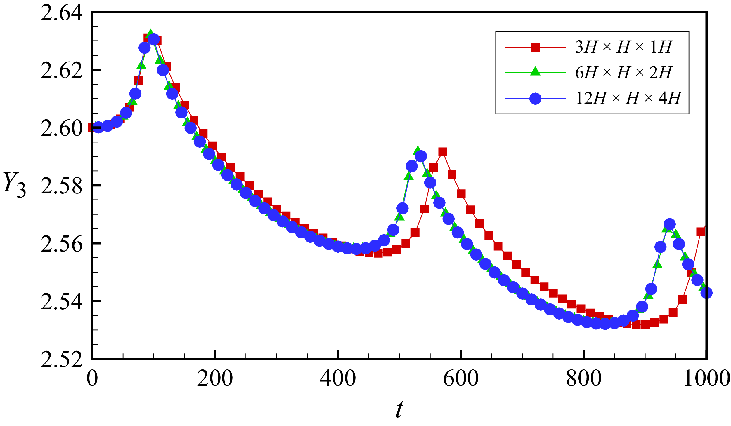
Evolution of the filament centroid position over time for different computational domain sizes (streamwise, wall normal, spanwise, with
 $H$
the channel height). At
 ${\textit{Re}}_c = 240$
and
 $\lambda = 1/8$
, the filament is initially aligned with the flow direction and placed at
 $Y_3|_{t=0} = 2.6$
, with its initial velocity equal to that of the undisturbed flow.

The flow field is discretised on a uniform Cartesian grid with spacing
 $\Delta x = 0.02$
. For
 ${\textit{Re}}_c \lt 200$
, a computational domain of
 $6H \times H \times 2H$
(streamwise, wall normal, spanwise, with
 $H$
the channel height) was verified to be sufficient to avoid spurious filament–filament interactions due to periodicity (figure 2). At higher Reynolds numbers (
 ${\textit{Re}}_c \in [200,2000]$
), longer-lived flow structures require an extended domain of
 $10H$
in the streamwise direction to suppress artificial periodic interactions.
No-slip boundary conditions on the channel walls are implemented via the half-way bounce-back scheme (Zou & He Reference Zou and He1997), while the fluid-filament no-slip condition is enforced using the IBM. To resolve fluid–structure interaction on the filament surface, 8 Lagrangian points are uniformly distributed in the circumferential direction and 128 along the axial direction. Unless otherwise specified, all simulations use filaments with aspect ratio
 $\kappa = 64$
and mass
 $M = 0.01$
.
3. Results and discussion
3.1. Finite
 ${\textit{Re}}_c$
model

A quasi-analytical solution for the regime
 ${\textit{Re}}_{\!f} \ll \mathcal{O}(1)$
and arbitrary
 ${\textit{Re}}_c$
can be derived using the method of asymptotic matching. Following the approach of Hogg (Reference Hogg1994) and Asmolov (Reference Asmolov1999), a Stokesian inner solution is constructed within the inertial screening length,
 $H{\textit{Re}}_c^{-1/2}$
, to satisfy the boundary conditions on the filament surface. When
 ${\textit{Re}}_c \gtrsim \mathcal{O}(1)$
, the inertial screening length becomes comparable to or smaller than the channel height
 $H$
, requiring an outer region where inertial effects are retained. The inner and outer solutions are then matched asymptotically. In the outer region, inertial and viscous forces are of comparable magnitude, and the solution satisfies the boundary conditions at the channel walls and in the far field.
When the (2.1) and (2.2) are rewritten in a centroid-fixed translating frame (as shown in figure 1
b) moving with the filament’s centre at
 $\boldsymbol{u}_{\!f}$
 \begin{equation} \begin{aligned} & {\textit{Re}}_{\!f}^{1/2}{\textit{Re}}_c^{1/2}\left (\frac {\partial \boldsymbol{w}}{\partial t}+\frac {\partial \boldsymbol{u}_s}{\partial t}+\boldsymbol{w} \boldsymbol{\cdot }\boldsymbol{\nabla } \boldsymbol{w}+\overline {\boldsymbol{u}} \boldsymbol{\cdot }\boldsymbol{\nabla } \boldsymbol{w}+\boldsymbol{w} \boldsymbol{\cdot }\boldsymbol{\nabla } \overline {\boldsymbol{u}}\right )=-\boldsymbol{\nabla }\left (p-p^{\infty }\right )+ {\nabla} ^{ 2} \boldsymbol{w}, \end{aligned} \end{equation}
where
 $\boldsymbol{w}$
represents the disturbance velocity caused by the presence and motion of the filament, while
 $\overline {\boldsymbol{u}}=(\alpha +\beta r_3+\gamma r_3^2)\boldsymbol{e}_1-\boldsymbol{u}_{\!f}$
denotes the undisturbed flow velocity in the body-fixed translating coordinate system and
 $\boldsymbol{u}_s=\alpha \boldsymbol{e}_1-\boldsymbol{u}_{\!f}$
represents the slip velocity. Here,
 $\alpha =4s(1-s)$
denotes the undisturbed velocity at the CoM of the filament,
 $\beta =4(1-2s)\lambda$
is the local shear rate depending on position and
 $\gamma =-4\lambda ^2$
is a constant characterising the shear gradient of the undisturbed flow. The disturbance velocity
 $\boldsymbol{w}$
satisfy the following conditions:
 \begin{equation} \begin{aligned} & \boldsymbol{\nabla }\boldsymbol{\cdot }\boldsymbol{w}=0, \\ & \boldsymbol{w}=\boldsymbol{\omega }_{\!f} \wedge \boldsymbol{r}-\bar {\boldsymbol{u}}, \quad \text{ on }\partial V_{\!f} \text{, }, \\ & \boldsymbol{w}=0, \quad r_3=-\lambda ^{-1}s, \lambda ^{-1}(1-s), \\ & \boldsymbol{w} \rightarrow 0, \quad |\boldsymbol{r}| \rightarrow \pm \infty , \\ & \int _{\partial V_{\!f}}(\sigma (\boldsymbol{w})+\sigma (\bar {\boldsymbol{u}})) \boldsymbol{\cdot }n \textrm{ d} S=\frac {2\pi St_g}{\lambda \kappa ^2} \frac {\textrm{d} \boldsymbol{u}_{\!f}}{\textrm{ d} t} . \end{aligned} \end{equation}
We now examine the relative magnitudes of the terms in (3.1). In this case, the disturbance flow scales as
 $\boldsymbol{w} \sim \beta /r^2 + \gamma /r^3$
, while the slip velocity scales as
 $\boldsymbol{u}_s \sim \gamma$
and we have undisturbed flow
 $\overline {\boldsymbol{u}} \sim \beta r +\gamma r^2$
. Under finite
 ${\textit{Re}}_G$
, the characteristic time for filament tumbling exceeds the Jeffery period, i.e.
 $T_{{\textit{Re}}} \gtrsim T_{{Jeff}} = 2\pi \beta ^{-1} (\kappa + \kappa ^{-1})$
(Jeffery Reference Jeffery1922; Rosén et al. Reference Rosén, Nordmark, Aidun, Do-Quang and Lundell2016)
 \begin{equation} \begin{aligned} \frac {\partial \boldsymbol{w}}{\partial t}+\frac {\partial \boldsymbol{u}_s}{\partial t} &\sim (\beta /r^2 + \gamma /r^3+\gamma )T_{{\textit{Re}}}^{-1},\quad \boldsymbol{w} \boldsymbol{\cdot }\boldsymbol{\nabla } \boldsymbol{w}+\overline {\boldsymbol{u}} \boldsymbol{\cdot }\boldsymbol{\nabla } \boldsymbol{w}+\boldsymbol{w} \boldsymbol{\cdot }\boldsymbol{\nabla } \overline {\boldsymbol{u}} \\ & \sim \beta ^2 / r^5+\beta \gamma / r^6+\gamma ^2 / r^7 + \beta ^2 / r^2+\beta \gamma / r+\gamma \beta / r^3+\gamma ^2 / r^2.\end{aligned} \end{equation}
Following the analysis paradigm of Anand & Subramanian (Reference Anand and Subramanian2024), we multiply (3.1) by the test function (
 $\sim ({1}/{r})$
) associated with a forcelet and integrate over a control volume with element
 $\textrm{d}V = O(r^2\,\textrm{d}r)$
. This integration yields the contribution of each term in (3.1) to the lateral migration velocity, thereby quantifying their respective roles
 \begin{equation} \begin{aligned} w^{(\textit{mig})}_{\textit{temporal}}&\sim (\beta \ln (r) + \gamma /r+\gamma r^2)T_{{\textit{Re}}}^{-1},\\ w^{(\textit{mig})}_{\textit{spatial}} &\sim \beta ^2 / r^3+\beta \gamma / r^4+\gamma ^2 / r^5 + \beta ^2 \ln r +\beta \gamma r +\gamma \beta / r+\gamma ^2 \ln r. \end{aligned} \end{equation}
Accounting for the finite filament size and the finite channel height, the radial coordinate is restricted to
 $r \in [1,\lambda ^{-1}]$
 \begin{equation} \begin{aligned} & w^{(\textit{mig})}_{\textit{temporal}}\sim (\beta (O(1)+\ln \lambda ^{-1}) + \gamma +\gamma \lambda ^{-2})T_{{\textit{Re}}}^{-1},\\ & w^{(\textit{mig})}_{\textit{spatial}} \sim \beta ^2 +\beta \gamma +\gamma ^2 / + \beta ^2 (O(1)+\ln \lambda ^{-1}) +\beta \gamma \lambda ^{-1} +\gamma \beta +\gamma ^2 (O(1)+\ln \lambda ^{-1}) .\end{aligned} \end{equation}
We first consider
 $w^{(\textit{mig})}_{\textit{temporal}}$
. The logarithmic contribution
 $\beta \ln \lambda ^{-1}T_{{\textit{Re}}}^{-1}$
arises from the matching region, whereas the term
 $\gamma T_{{\textit{Re}}}^{-1}$
arises from the inner region. Neither of these contributions generates any net lift upon period averaging. The occurrence of any net period-averaged migration necessarily depends on the boundary conditions, and therefore can only arise from the outer-region terms,
 $\beta T_{{\textit{Re}}}^{-1}$
and
 $\gamma \lambda ^{-2}T_{{\textit{Re}}}^{-1}$
. Further asymptotic analysis with respect to
 $\lambda$
shows that the leading-order contribution to
 $w^{(\textit{mig})}_{\textit{temporal}}$
is
 $\gamma \lambda ^{-2}T_{{\textit{Re}}}^{-1}$
. Here, the leading-order contribution of the temporal derivative term arises entirely from
 $\boldsymbol{u}_s$
. By performing the same analysis, we find that the dominant contributions to
 $w^{(\textit{mig})}_{\textit{spatial}}$
are
 $\beta ^2$
and
 $\beta \gamma \lambda ^{-1}$
, which arise from the linear terms in the disturbance velocity
 $\boldsymbol{w}$
. Therefore, the condition under which the time-derivative term can be neglected is simply
 \begin{equation} \begin{aligned} \lambda \kappa \gg 1, \end{aligned} \end{equation}
which is readily satisfied for slender filaments in most cases. However, in certain extreme situations – such as the case with
 $\lambda =1/32$
shown in figure 9 – noticeable discrepancies between the theoretical model and numerical simulations emerge when
 $\lambda \kappa =2$
.
3.1.1. The inner solution
In the inner region,
 ${\textit{Re}}_{\!f}$
is sufficiently small that the flow is governed by the Stokes equations. Under this regime, a slender-body approximation known as resistive-force theory (RFT) can be applied to compute the leading-order disturbance velocity induced by the filament (Kim & Karrila Reference Kim and Karrila2013). The velocity difference between the filament and the undisturbed background flow is decomposed into components parallel
 $\Delta \boldsymbol{u}_{\mathop {//}}(\xi )$
and perpendicular
 $\Delta \boldsymbol{u}_\perp (\xi )$
to the local filament axis. Here,
 $\xi$
is the body-fixed coordinate along the filament axis, as illustrated in figure 1(a). This decomposition forms the basis for approximating the distributed hydrodynamic force acting on the filament
 \begin{equation} \begin{aligned} \boldsymbol{f}_{\!f}(\xi )=&-\lambda _{1}\Delta \boldsymbol{u}_{\mathop {//}}(\xi )-\lambda _2\Delta \boldsymbol{u}_\perp (\xi ). \end{aligned} \end{equation}
The anisotropic hydrodynamic resistance of the filament is captured by two coefficients,
 $\lambda _1 = ( {2\pi \mu }/({\ln (2\kappa )-1/2}))$
,
 $\lambda _2 = ( {4\pi \mu }/({\ln (2\kappa )+1/2}))$
, which differ by roughly a factor of two for large aspect ratio
 $\kappa$
. The disturbance velocity in the inner region, at distances not extremely close to the filament (
 $|\boldsymbol{r}|\lt \mathcal{O}(a)$
) , can thus be expressed as a function of the force monopole
 $\boldsymbol{F}$
and force dipole
 $\boldsymbol{D}$
exerted by the filament on the surrounding fluid
 \begin{equation} u_i(\boldsymbol{r})-\overline {u}_i(\boldsymbol{r})=\frac {F_{fl}}{8\pi \mu }\mathcal{G}_{il}(\boldsymbol{r})+\frac {D_{fjk}}{8 \pi \mu } \mathcal{G}_{ij,k}(\boldsymbol{r}), \end{equation}
where
 $\mathcal{G}_{i j}=( {1}/{r}) \delta _{i j}+( {1}/{r^3}) x_i x_j, r=|\boldsymbol{x}|$
is the Oseen tensor, and
 $\mathcal{G}_{i j, k}=( {1}/{r^3}) (-\delta _{i j} x_k+\delta _{j k} x_i+\delta _{i k} x_j )-( {3}/{r^5}) x_i x_j x_k$
is the spatial derivative of the Oseen tensor. Further details and explicit expressions for
 $\boldsymbol{F}_{\!f}$
and
 $\boldsymbol{D}_{\!f}$
are provided in Appendix B. It is worth noting here that our analysis is restricted to filament motions confined to the flow-shear plane, since fluid inertia tends to drive slender filaments, regardless of their initial orientation, toward the degenerate Jeffery orbit characterised by an orbit constant
 $C=\infty$
(Subramanian & Koch Reference Subramanian and Koch2005). As a result,
 $\boldsymbol{F}_{\!f}$
depends on
 $\boldsymbol{u}_{\!f}$
,
 $s$
and
 $\phi$
, while
 $\boldsymbol{D}_{\!f}$
additionally depends on the angular velocity
 $\omega _{\!f}$
.
3.1.2. The outer solution
If the inertial screening length of the filament is smaller than
 $H$
, the viscous force term and the advective terms due to undisturbed shear velocity in the outer region are matched. By introducing a linear scaling
 \begin{equation} \boldsymbol{R}=\epsilon \boldsymbol{r}. \end{equation}
Following Saffman’s (Reference Saffman1965) approach, the matching conditions can be incorporated into the momentum equation by introducing appropriate forcing terms. This leads to the governing equation for the outer solution region
 \begin{align} &{\textit{Re}}_{\!f}^{1/2}{\textit{Re}}_c^{1/2}\left(\frac {\partial \boldsymbol{W}}{\partial t}\right.+\frac {\partial \boldsymbol{U}_s}{\partial t}+\epsilon \boldsymbol{W} \boldsymbol{\cdot }\boldsymbol{\nabla }\boldsymbol{W}+\underbrace {\epsilon (\bar {\boldsymbol{U}}-\boldsymbol{U}_s) \boldsymbol{\cdot }\boldsymbol{\nabla }\boldsymbol{W}+\epsilon \boldsymbol{W} \boldsymbol{\cdot }\boldsymbol{\nabla }(\bar {\boldsymbol{U}}-\boldsymbol{U}_s)}_{\text{inertia } 1}\nonumber\\ &\quad +\underbrace {\epsilon \boldsymbol{U}_s \boldsymbol{\cdot }\boldsymbol{\nabla }\boldsymbol{W}}_{\text{inertia } 2}\Big)=-\epsilon \boldsymbol{\nabla }P+\underbrace {\epsilon ^2 \boldsymbol{\nabla} ^2 \boldsymbol{W}}_{\text{viscous }} +\epsilon ^2\boldsymbol{F}_{\!f}\delta (\boldsymbol{R})+\epsilon ^4\boldsymbol{D}_{\!f}\boldsymbol{\cdot }\boldsymbol{\nabla }\delta (\boldsymbol{R}) .\end{align}
Assuming that the convective term induced by the undisturbed flow (inertia 1) significantly exceeds that arising from filament migration (inertia 2), the former must balance the viscous term (viscous). This yields the primary perturbation parameter for the problem
 \begin{equation} \epsilon ={\textit{Re}}_{\!f}^{1/2}. \end{equation}
Therefore, the disturbance velocity field and pressure must satisfy
 \begin{equation} \boldsymbol{w}=\epsilon ^3 \boldsymbol{W} + o(\epsilon ^3), \quad p=\epsilon ^4P+o(\epsilon ^4). \end{equation}
By performing a two-dimensional Fourier transform parallel to the upper and lower walls, we obtain
 \begin{equation} \begin{aligned} & \left \{\begin{array}{l} \tilde {\boldsymbol{W}}(k_1, k_2, R_3) \\ \tilde {\boldsymbol{P}}(k_1, k_2, R_3) \end{array}\right \}=\frac {1}{4 \pi ^2} \int _{-\infty }^{\infty } \int _{-\infty }^{\infty }\left \{\begin{array}{l} \boldsymbol{W}(R_1, R_2, R_3) \\ \boldsymbol{P}(R_1, R_2, R_3) \end{array}\right \} \textrm{e}^{-i\left (k_1 R_1+k_2 R_2\right )} \textrm{d} R_1 \textrm{ d} R_2 . \\ \end{aligned} \end{equation}
If the transient effects are considered small, the first two terms in (3.10) can be neglected. Similarly, applying a two-dimensional Fourier transform yields
 \begin{equation} \begin{aligned} \textrm{L}\tilde {\boldsymbol{W}}&=\boldsymbol{k}\tilde {P}+\left (\beta R_3-4 {\textit{Re}}_c^{-1/2} R_3^2\right ) \textrm{i} k_1 \tilde {\boldsymbol{W}}+\big(\beta -8 {\textit{Re}}_c^{-\frac {1}{2}} R_3\big) \tilde {W_3} \boldsymbol{e}_1 \\ &\quad +\frac {1}{4 \pi ^2} {\textit{Re}}_c^{\frac {1}{2}} (\boldsymbol{F}_{\!f} \delta (R_3)+\boldsymbol{D}\boldsymbol{\cdot }\boldsymbol{k}^T \delta (R_3)), \\ \textrm{L}\tilde {P}&=-2 \textrm{i} k_1\big(\beta -8 {\textit{Re}}_c^{-\frac {1}{2}} R_3\big) \tilde {W}_3-\frac {1}{4 \pi ^2} {\textit{Re}}_c^{\frac {1}{2}} (\boldsymbol{F}_{\!f} \boldsymbol{\cdot }\boldsymbol{k}^T + \boldsymbol{k}\boldsymbol{\cdot }\boldsymbol{D}_{\!f}\boldsymbol{\cdot }\boldsymbol{k}^T)\delta (R_3), \\ \end{aligned} \end{equation}
and the boundary conditions of the upper and lower walls must still be satisfied
 \begin{equation} \begin{aligned} & \tilde {\boldsymbol{W}}=0, \quad R_3=-{\textit{Re}}_c^{\frac {1}{2}} s, {\textit{Re}}_c^{\frac {1}{2}}(1-s) .\\ \end{aligned} \end{equation}
Here,
 $\boldsymbol{k} = (k_1, k_2, \partial / \partial R_3)$
represents the wave vector. Note that
 $k_1$
and
 $k_2$
denote the Fourier wavenumbers in the streamwise and spanwise directions, while the wall-normal direction is left in physical space, so the third component remains as the differential operator
 $\partial /\partial R_3$
. The governing equation can be formulated as the following fourth-order ordinary differential equation for the Fourier transform of the lateral velocity:
 \begin{equation} \begin{aligned} \big(\textrm{L}^2-\textrm{i} k_1 \bar {V}_1 \textrm{ L}-\textrm{i} k_1 8 {\textit{Re}}_c^{-1 / 2}\big) \widetilde {W}_3=-\frac {{\textit{Re}}_c^{1/2}}{4\pi ^2}\left [d^{(0)}\delta (R_3)+d^{(1)}\frac {{\textrm d}\delta (R_3)}{{\textrm d}R_3}+d^{(2)}\frac {d^2\delta (R_3)}{{\textrm d}R_3^2} \right ]\!, \end{aligned} \end{equation}
that satisfies the no-slip boundary condition at the wall
 \begin{equation} \begin{aligned} \widetilde {W}_3=\frac {\textrm{d} \widetilde {W}_3}{\textrm{ d} R_3}=0 \quad \text{ on } \quad R_3=-{\textit{Re}}_c^{1 / 2} s, \quad {\textit{Re}}_c^{1 / 2}(1-s), \end{aligned} \end{equation}
where
 \begin{equation} \textrm{L}=\frac {\textrm{d}^2}{\textrm{ d} R_3^2}-k^2, \quad k^2=k_1^2+k_3^2. \end{equation}
The delta function and its derivatives in the right end term can be written as jump conditions
 \begin{equation} \begin{aligned} \left [ \frac {{\textrm d}\widetilde {W}_3}{{\textrm d}R_3}\right ]&=-\frac {{\textit{Re}}_c^{-1/2}}{4\pi ^2}d^{(2)},\\ \left [ \frac {\textrm{d}^2\widetilde {W}_3}{{\textrm d}R_3^2}\right ]&=-\frac {{\textit{Re}}_c^{-1/2}}{4\pi ^2}d^{(1)},\\ \left [ \frac {\textrm{d}^3\widetilde {W}_3}{{\textrm d}R_3^3}\right ]&=-\frac {{\textit{Re}}_c^{-1/2}}{4\pi ^2}d^{(3)},\\ \end{aligned} \end{equation}
where
 $ [f ]=f(k_1,0^+,k_3)-f(k_1,0^-,k_3)$
is the magnitude of the jump, and
 \begin{align} \bar {V}_1&={\textit{Re}}_c^{1/2}\boldsymbol{U}_s+\beta R_3+ R_c^{-1 / 2} \beta R_3^2, \end{align}
 \begin{align} d^{(0)}&=k^2F_{f3}+ik_1k^2D_{\!f31},\nonumber\\ d^{(1)}&=ik_1F_1-k_1^2D_{f11}+k^2D_{f33},\nonumber\\ d^{(2)}&=ik_1D_{f13},\nonumber\\ d^{(3)}&=k^2(2ik_1D_{f13}+F_{f3}+ik_1D_{f31}). \end{align}
In the absence of gravity, the term
 $\boldsymbol{F}_{\!f}$
arises solely from the last term in (3.2), representing the solid inertial force. Here, we neglect the contribution of
 $\boldsymbol{F}_{\!f}$
, as it is significantly smaller than that of
 $\boldsymbol{D}_{\!f}$
in determining
 $W_3^{({mig})}$
for slender bodies. The effect of solid inertia will be considered later in (3.30).
The wavenumber-dependent migration velocity
 $\tilde {W}_3(k_1, k_2, R_3)$
is obtained by numerically solving the governing (3.16) subject to the specified jump conditions (3.19). However, conventional finite difference methods become unstable or inaccurate for
 ${\textit{Re}}_c \gt 100$
, even with very fine integration step sizes. Previous studies have demonstrated the robustness of orthogonalisation techniques (Asmolov Reference Asmolov1999; Anand & Subramanian Reference Anand and Subramanian2023) in handling cases up to
 ${\textit{Re}}_c \approx 3000$
. To further improve numerical stability and efficiency, we adopt an adaptive implicit Runge–Kutta method based on the five-stage Lobatto IIIC* formula (Dekker Reference Dekker1984; Wanner & Hairer Reference Wanner and Hairer1996). The complete algorithm is provided in Appendix C. The corresponding lateral disturbance velocity at the filament centroid in physical space is then recovered via inverse Fourier transform
 \begin{equation} W_{3}^{(\textit{mig})}= {{\textrm{Re}}}\left [\left .\int _{0}^{2\pi } \int _{0}^{\infty }\widetilde {W}_3\right |_{R_3 \rightarrow 0} k\textrm{ d} k \textrm{ d} \theta \right ]\! . \end{equation}
Here,
 $ {\textrm{Re}}[ \boldsymbol{\cdot }]$
denotes the real part of a complex number. The integration in (3.22) is performed numerically using Gauss–Legendre quadrature in the plane polar coordinates
 $ (k, \theta )$
, rather than in the Cartesian coordinates
 $ (k_1, k_2)$
, where
 $\theta =\arccos (k_1/k)$
. As noted in Appendix D, for sufficiently large
 $k$
, the solution to (3.16) exhibits exponential decay away from the origin. By treating
 $k^{-1}$
as a perturbation parameter, the migration velocity in the large-wavenumber limit can be obtained
 \begin{equation} \textit{Re} \left [\widetilde {W}_3\left (k, \theta , 0\right )\right ]=\frac {3(D_{f13}+5 D_{f31})\cos ^2\theta }{32\pi ^2 {\textit{Re}}_c k^3}+O(k^{-4}) \quad \text{ as } \quad k \rightarrow \infty . \end{equation}
The final lateral migration velocity is composed of the numerical solution for
 $k\lt K_m$
and the asymptotic solution for
 $k\gt K_m$
 \begin{equation} W_{3}^{(\textit{mig})}= \textit {Re}\left [\left .\int _{0}^{2\pi } \int _{0}^{K_m}\widetilde {W}_3\right |_{R_3 \rightarrow 0} k\textrm{ d} k \textrm{ d} \theta \right ] +\frac {3(D_{f13}+5 D_{f31})}{64\pi {\textit{Re}}_c K_m^2}+O\big(K_m^{-3}\big), \end{equation}
where
 $K_m$
is a cutoff radius used to control the numerical accuracy of the computation. It has been verified that, for the range of Reynolds numbers considered in this study,
 $K_m=128$
provides sufficient accuracy for
 $s\in [0.04,0.96]$
.
3.2. Simplification for fixed inclination angles
We begin by examining a simplified case in which the filament maintains a fixed orientation (
 $\phi = \pi /4$
) but is still free to translate within the channel. This set-up artificially decouples translational and rotational dynamics by applying an external torque – an approach that does not reflect typical flow conditions but serves as a useful idealisation. Analysing this constrained scenario allows us to isolate the effect of unsteady angular motion on lateral migration and provides valuable insights into the limitations of the present theory.
At
 ${\textit{Re}}_c=40$
and
 $\phi =\pi /4$
, the migration velocity of filament with a fixed inclination angle. Panels (a), (b), (c) and (d) illustrate different segments of the same lift-force profile.

Figure 3 compares the lateral migration velocity of a filament inclined at
 $\phi = \pi /4$
, obtained from the quasi-analytical solution of (3.16), with results from LBM simulations. Both approaches exhibit a distinct ‘bathtub-shaped’ velocity profile: the migration velocity is high near the walls (
 $s = 0$
to
 $0.1$
and
 $0.9$
to
 $1$
) and much lower in the central region of the channel. This behaviour is clearly visible in the zoom-in view in figure 3(c). Notably, for
 $\lambda = 1/64$
, the LBM data near both the lower wall (
 $s = 0$
to
 $0.2$
) and upper wall (
 $s = 0.8$
to
 $1$
) closely match the analytical prediction, providing a strong initial validation of the theoretical model.
This bathtub-shaped profile differs markedly from the antisymmetric S-shaped migration velocity typical of inertially migrating spherical particles (Anand & Subramanian Reference Anand and Subramanian2024). For spheres, symmetry in both geometry and flow leads to symmetric inertial forces near the upper and lower walls, generally resulting in equal repulsive effects from both boundaries. In contrast, inclined filaments break this symmetry. As shown in figure 3(b), a filament tilted upward at
 $\phi = \pi /4$
experiences a positive (upward) migration velocity near both the lower and upper walls. Since inertial forces align with the migration direction, the filament is pushed away from the lower wall but pulled toward the upper wall. Importantly, this force becomes stronger as the filament approaches either wall. Consequently, the model predicts that a filament released near the upper wall may be attracted toward it, potentially leading to wall contact.
While the theoretical and LBM results show good agreement near the walls in the weakly confined case (
 $\lambda = 1/64$
), near-wall data are unavailable for more strongly confined cases with larger
 $\lambda$
. This is due to geometric constraints: the filament tip makes contact with the wall, preventing reliable data collection in these regions. For instance, with
 $\lambda = 1/16$
and
 $\phi = \pi /4$
, the filament centre reaches
 $s = 1 - \lambda \cos (\pi /4) \approx 0.912$
just before the tip touches the upper wall, so no LBM data are available for
 $s \gt 0.912$
. Near-wall dynamics such as lubrication forces and post-collision behaviours known as ‘pole vaulting’ may then arise (Dhanasekaran & Koch Reference Dhanasekaran and Koch2019; Teng et al. Reference Teng, Rallabandi, Stone and Ault2022; Wilkinson, Pradas & Wilkinson Reference Wilkinson, Pradas and Wilkinson2023). Although these effects are intriguing, they lie beyond the scope of the present study.
When the distance between the wall and the filament centroid becomes very small (smaller than the inertial screening length) but before solid–solid contact occurs, the singular perturbation method employed here ceases to be valid. In this regime, LBM simulations indicate that, for a fixed inclination angle of
 $\phi = \pi /4$
, the filament continues to accelerate toward the upper wall until contact takes place. Once collision occurs, the lateral migration velocity necessarily switches to zero or even negative values, depending on frictional effects that lie beyond the scope of the present study. It should also be noted that the interaction of a freely rotating filament with a single wall in linear shear flow has been specifically analysed by Dhanasekaran & Koch (Reference Dhanasekaran and Koch2019), who showed that when the wall–centroid distance falls below the inertial screening length, the freely rotating filament experiences a repulsive force from the wall.
In the central region of the channel, as shown in figure 3(c), both the theoretical model and LBM simulations predict significantly lower migration velocities compared with the near-wall regions. However, the predicted equilibrium positions differ. The theoretical model suggests a stable equilibrium at the channel centre
 $s = 0.5$
, as shown in figure 3(d), while the LBM simulations indicate a stable position closer to the lower wall. For example, at
 $\lambda = 1/16$
, the equilibrium position is around
 $s = 0.4$
. This discrepancy is discussed in detail in Appendix E. In short, it is due to a limitation of the current theoretical model, which considers only the effect of local shear rate. Since the shear rate vanishes at the centreline, the model fails to capture the influence of the shear gradient, which remains constant throughout the channel and becomes the dominant factor driving migration near the centre.
At (a)
 ${\textit{Re}}_c=40$
and (b)
 ${\textit{Re}}_c=1000$
, the migration velocity
 $W_3^{(\textit{mig})}$
of a filament with different
 $\phi$
. The cases
 $\phi =0$
and
 $\phi =9\pi /18$
correspond to trivial solutions that are identically zero and therefore are not shown.

To further explore the influence of inclination angle
 $\phi$
on migration behaviour, figure 4 presents theoretical predictions for
 $\lambda =1/64$
at various angles. For
 $\phi = 1\pi /18$
, four equilibrium positions emerge: two stable equilibria at
 $s = 0.39$
and
 $s = 0.88$
, and two unstable equilibria at
 $s = 0.50$
and
 $s = 0.70$
for
 ${\textit{Re}}_c = 40$
(figure 4
a). Results for higher Reynolds numbers up to
 ${\textit{Re}}_c = 1000$
are shown in figure 4(b).
3.3. Case of torque-free dynamics
In this section, we examine the migration behaviour of a freely rotating filament in a channel under zero external torque. Specifically, we compute the lateral disturbance velocity
 $W_3^{({mig})}$
in the
 $\phi - s$
plane under the torque-free condition
 $T_{\!f} = 0$
, using (3.24). The detailed numerical procedure and parameter settings are provided in Appendix C, with the resulting lateral migration-velocity profile shown in figure 5(a). If a dashed line is drawn at
 $\phi = \pi /4$
, the resulting cross-section resembles the profile in figure 3. The velocity field in the
 $\phi - s$
plane is antisymmetric about both
 $(\phi , s) = (0, 0.5)$
and
 $(0.5, 0.5)$
, remains relatively flat near the channel centre and increases sharply near the walls.
(a) Lateral disturbance velocity
 $W_3^{(\textit{mig})}$
and (b) streamwise disturbance velocity
 $W_1^{(\textit{mig})}$
at
 ${\textit{Re}}_c=24$
.

Unlike isotropic spherical particles, the filament’s anisotropy and finite inertia induce a coupling between the lateral migration velocity and the streamwise disturbance velocity
 $W_1^{({mig})}$
. As in the previous subsection, the governing equation for the Fourier-transformed streamwise disturbance velocity
 \begin{align} L\widetilde {W}_1&= ik_1 \widetilde {P} +\left (\beta R_3-4 R_c^{-1/2} R_3^2\right )ik_1\widetilde {W}_1+ \left (\beta -8 R_c^{-\frac {1}{2}} R_3\right )\widetilde {W}_3 \nonumber\\ &\quad -\frac {{\textit{Re}}_c^{-1/2}}{4\pi ^2}(ik_1D_{f13}+D_{f33}\frac {\partial }{\partial R_3})\delta (R_3), \end{align}
 \begin{align} \frac {\partial \widetilde {P}}{\partial R_3}&= \frac {\partial ^2 \widetilde {W}_3}{\partial R_3^2}-k^2 \widetilde {W}_3 - \left (\beta R_3-4 R_c^{-1/2} R_3^2\right )ik_1\widetilde {W}_3 \nonumber\\ &\quad -\frac {{\textit{Re}}_c^{-1/2}}{4\pi ^2}\left(-ik_1D_{f31}-D_{f33}\frac {\partial }{\partial R_3}\right)\delta (R_3), \end{align}
and the corresponding jump condition at the origin can be derived
 \begin{align} \left [ \widetilde {W}_1 \right ]&=-\frac {{\textit{Re}}_c^{-1/2}}{4\pi ^2}D_{f33}, \end{align}
 \begin{align} \left [ \frac {{\textrm d}\widetilde {W}_1}{{\textrm d}R_3}\right ]&=-\frac {{\textit{Re}}_c^{-1/2}}{4\pi ^2}ik_1D_{f13}, \end{align}
 \begin{align} \left [\widetilde {P}\right ]&=-\frac {{\textit{Re}}_c^{-1/2}}{4\pi ^2}ik_1(D_{f13}-D_{f31}). \end{align}
The numerical solution of the governing equation at
 ${\textit{Re}}_c=24$
is shown in figure 5(b). The results reveal that the streamwise disturbance velocity is strongly dependent on the filament’s orientation
 $\boldsymbol{p}$
, underscoring the need for a detailed examination of the filament’s orientational dynamics. In an unbounded linear shear Stokes flow, a slender filament undergoes periodic tumbling motion along a Jeffery orbit (Jeffery Reference Jeffery1922). The orbit-averaged migration velocity of ellipsoidal particles with arbitrary aspect ratios has been analysed in the work of Anand & Subramanian (Reference Anand and Subramanian2023). However, to the best of our knowledge, the full-period oscillatory migration behaviour of a filament has not been systematically studied, making it a central focus of this section.
Another key aspect explored here is the role of a small but finite shear Reynolds number
 ${\textit{Re}}_G$
, which introduces an
 $\mathcal{O}({\textit{Re}}_G)$
correction to the rotational velocity
 $\dot {\phi }$
. This correction alters the filament’s orientational dynamics and can significantly influence its period-averaged lateral equilibrium position.
To capture both orientation and translation, we now formulate a coupled system of differential equations. This system extends the classical equation for the azimuthal angle used by Lundell & Carlsson (Reference Lundell and Carlsson2010) and Bagge et al. (Reference Bagge, Rosén, Lundell and Tornberg2021) for prolate spheroidal particles by incorporating the following evolution of the filament’s centroid position in addition to its angular dynamics:
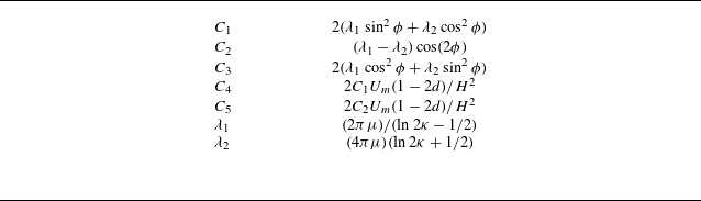
 \begin{equation} \frac {\textrm{d}^2}{{\textrm d}t^2} \begin{bmatrix} Y_{1} \\ Y_{3} \\ \phi \end{bmatrix} =\frac {1}{M} \begin{bmatrix} F_{f1}-C_1aW_1^{(\textit{mig})}\epsilon ^3-C_2aW_3^{(\textit{mig})}\epsilon ^3 \\[5pt] F_{f3}-C_2aW_1^{(\textit{mig})}\epsilon ^3-C_3aW_3^{(\textit{mig})}\epsilon ^3 \\[5pt] 3a^{-2}T_{f2}+2\lambda _2a\dot {\phi }^{(corr)} \end{bmatrix}\!. \end{equation}
The detailed expressions for the force
 $\boldsymbol{F}_{\!f}$
, torque
 $\boldsymbol{T}_{\!f}$
acting on the filament and the coefficient
 $C_\alpha$
are provided in Appendix B. Notably, the term
 $\dot {\phi }^{(\textit{corr})}$
in the system of equations represents a correction to the filament’s angular velocity arising from finite
 ${\textit{Re}}_G$
effects. For
 ${\textit{Re}}_G = \mathcal{O}(1)$
or smaller, an analytical expression for this correction has been derived by Rosén et al. (Reference Rosén, Nordmark, Aidun, Do-Quang and Lundell2016), with a brief summary included in Appendix F.
Equation (3.30) is integrated using CVODE from the SUNDIALS suite, whose variable-step, variable-order Backward Differentiation Formulas schemes are well suited to the stiffness arising from the small filament mass
 $M$
, efficiently resolving both weak-force near-alignment phases and the sharp transients during tumbling. When taking the limits
 ${\textit{Re}}_{\!f} \to 0$
and
 $St_g \to 0$
, the computed migration velocities reduce to the Jeffery-orbit-averaged results obtained by Anand & Subramanian (Reference Anand and Subramanian2023), despite differences in methodological approach. A key advantage of the present formulation is its ability to capture the oscillatory motion of the filament’s centroid throughout an entire tumbling period, providing richer dynamical insight beyond orbit-averaged quantities.
Comparison between LBM numerical simulations (purple solid lines) and perturbation method predictions (green solid lines) for a filament at
 ${\textit{Re}}_c=24$
: (a) lateral position of the filament’s CoM. Here, the red annotation is used to highlight that the range of the horizontal axis differs from that in the other panels; (b) streamwise velocity of the CoM; (c) lateral velocity of the CoM; (d) angular velocity in the vorticity plane; (e) polar plot of the transverse migration velocity as a function of filament orientation. In this plot, the azimuthal angle corresponds to the circumferential coordinate, the migration velocity
 $\dot {Y}_3$
is plotted along the radial axis and the grey dashed circle indicates the zero-migration-velocity contour; (f) lateral position of the filament as a function of its orientation angle.

Figure 6(a) compares the lateral position of the filament’s CoM
 $Y_3$
, released at
 $Y_3|_{t=0} = 5.8$
with an initial orientation of
 $\phi = \pi /2$
, for
 $\lambda = 1/16$
and
 ${\textit{Re}}_c = 24$
, as obtained from both the numerical integration of (3.30) and LBM simulations. Although the trajectories are not perfectly synchronised in time (with the LBM showing a slightly shorter tumbling period than the analytical solution), both methods consistently capture the filament’s complex oscillatory motion during half a tumbling cycle, characterised by two local maxima and two local minima. Eventually, both approaches predict that the filament enters a quasi-equilibrium tumbling state, characterised by sustained rotation and lateral oscillation about a stable transverse position (not shown here). To better illustrate this oscillatory behaviour, figure 6(f) plots
 $Y_3$
as a function of the filament’s orientation angle
 $\phi$
. In this representation, the locations of the local maxima and minima predicted by both methods are well aligned, highlighting their agreement in the angular dependence of the lateral migration.
Same as figure 6, but for
 ${\textit{Re}}_c=800$
,
 $\lambda =1/16$
.

Figure 6(b) shows the streamwise velocity
 $\dot {Y}_1$
of the filament. For most of the tumbling period, the velocity curve remains nearly flat, resembling a horizontal line. However, each period features a distinct valley where the streamwise velocity drops sharply. These valleys correspond to moments when the filament is oriented perpendicular to the flow, causing a reduction in the centroid velocity. In contrast, the velocity reaches a local maximum when the filament aligns with the flow direction – approaching the undisturbed fluid velocity at its centroid. While this peak is relatively subtle, it is observable; for example, the LBM result peaks around
 $t \approx 434$
, and the analytical prediction peaks near
 $t \approx 535$
.
Figure 6(c) shows the lateral (wall-normal) velocity of the filament’s centroid. When the filament is approximately aligned with the flow direction, the transverse migration velocity remains relatively small but persists over most of the tumbling period. In contrast, when the filament becomes nearly perpendicular to the flow, the migration velocity exhibits a sharp peak – brief but significantly larger in magnitude. Notably, the analytical solution underestimates the peak velocity compared with the LBM simulation.
Figure 6(d) presents the evolution of the angular velocity. As expected from Jeffery’s theory (Jeffery Reference Jeffery1922), the angular velocity approaches minima when the filament aligns with the flow and reaches a maximum when the filament is perpendicular to it.
The dependence of the lateral migration velocity on the filament’s orientation angle is further illustrated in figure 6(e). For clarity, figure 6(e) shows only the trajectory of the filament after it has reached its quasi-equilibrium position, represented as a limit cycle. This plot confirms a strong angular dependence and reinforces the trend observed in panel (c): the perturbation method systematically underpredicts the amplitude of the velocity. Nevertheless, it accurately captures the locations of the extrema, with the two maxima occurring at
 $\phi \approx 0.350\pi$
and
 $\phi \approx 0.824\pi$
, and the two minima at
 $\phi \approx 0.094\pi$
and
 $\phi \approx 0.564\pi$
.
At a significantly higher Reynolds number (
 ${\textit{Re}}_c = 800$
), figure 7 shows the same quantities. As seen in figures 7(a) and 7(f), a key difference emerges: after being released at
 $Y_3|_{t=0} = 7$
, the filament undergoes roughly
 $0.96\pi$
of rotation before halting. It then maintains a nearly fixed inclination angle for a prolonged period while migrating laterally. Rotation resumes only as the filament nears its equilibrium position. This behaviour results from the non-uniform local Reynolds number
 ${\textit{Re}}_G$
. A similar phenomenon was observed by Aidun, Lu & Ding (Reference Aidun, Lu and Ding1998), who found that filaments in uniform shear flow stop tumbling at high
 ${\textit{Re}}_G$
, then resume rotation as
 ${\textit{Re}}_G$
decreases.
Compared with the low-
 ${\textit{Re}}_c$
case in figure 6, discrepancies between the theoretical predictions and LBM simulations are more pronounced at
 ${\textit{Re}}_c = 800$
. This is due to the inertial screening length (
 $H{\textit{Re}}_c^{-1/2}\approx 0.57a$
) becoming smaller than the length of filament’s semi-major axis
 $a$
, rendering both the singular perturbation method and RFT invalid under these conditions.
The period-averaged migration velocity of the filament at
 ${\textit{Re}}_c=300$
.

Figure 8 shows the dependence of the period-averaged lateral migration velocity of a filament under moderate Reynolds number (
 ${\textit{Re}}_c = 300$
) and moderate channel confinement (
 $\lambda = 1/16$
). The averaging operation is defined as
 $\langle \boldsymbol{\cdot }\rangle _T=({1}/{\mathcal{T}})\int _t^{t+\mathcal{T}} (\boldsymbol{\cdot }),{\textrm d}t$
, where
 $\mathcal{T}$
denotes the tumbling period. The vertical axis is non-dimensionalised using the scaling
 $\kappa \ln (\kappa )$
, as proposed by (Anand & Subramanian Reference Anand and Subramanian2023). The grey solid line represents their analytical solution in the limit
 ${\textit{Re}}_{\!f} \rightarrow 0$
, while the purple circles and green solid line correspond to results from our LBM simulations and theoretical model, respectively.
Overall, our theoretical predictions (green curve) show good qualitative consistency with the LBM data (purple circles), particularly in identifying the equilibrium location at
 $s \approx 0.63$
. However, quantitative differences remain, especially at larger
 $s$
, where the predicted migration velocity departs from the simulation results. Compared with the model of Anand & Subramanian (Reference Anand and Subramanian2023), our framework provides improved agreement near the channel centre and correctly predicts the equilibrium closer to the centreline.
To better understand the differences, we note that near the channel centre (
 $s \to 0.5$
), the shear Reynolds number
 ${\textit{Re}}_G$
approaches zero, causing the inertial correction term
 $\dot {\phi }^{(\textit{corr})}$
to vanish. This explains why the two asymptotic methods converge to the same limit, and within this interval the LBM simulation results are also in reasonable agreement with the perturbation theory. It should be emphasised, however, that a finite-size filament located exactly at the centreline would not generally exhibit strictly zero migration: except for the perfectly symmetric cases where the filament is aligned exactly parallel or perpendicular to the flow, weak migration persists due to shear-gradient effects. Since the present asymptotic model accounts only for the local velocity gradient at the filament centroid, this shear-gradient contribution is not captured, and the prediction of vanishing migration at the centreline should be interpreted within this limitation.
As
 $s\gt 0.56$
,
 ${\textit{Re}}_G$
grows and the correction term
 $\dot {\phi }^{(\textit{corr})}$
can no longer be neglected, leading to a substantial divergence between the two asymptotic approaches. The model of Anand predicts a relatively flat and positive migration-velocity curve, reaching equilibrium only at
 $s=0.87$
. By contrast, our model, which incorporates finite
 ${\textit{Re}}_G$
corrections, is in much closer agreement with the LBM simulations in the range
 $s = 0.56$
–
 $0.79$
, and also predicts an equilibrium position nearer to the simulation result (
 $s \approx 0.63$
). With further increase of
 $s$
, in the near-wall region (
 $s \gt 0.79$
), neither asymptotic model is able to capture the trend observed in the LBM data, because the distance between the filament centre and the wall becomes comparable to the filament half-length, and higher-order wall-induced hydrodynamic interactions – beyond the scope of the present asymptotic treatments – become dominant. A more refined theoretical framework would therefore be required to resolve this near-wall regime.
Further analysis of the equilibrium position is provided in figure 9. Another important implication of figure 8 is that previous theoretical approaches may have substantially underestimated the period-averaged migration velocity of slender filaments. This, in turn, could lead to an overestimation of the entrance length required for full lateral migration.
The variation of the filament’s equilibrium position with
 ${\textit{Re}}_c$
for different values of
 $\lambda$
is presented.

A major outcome of this study is the development of a physically grounded theoretical framework that predicts the equilibrium position of a finite-sized filament undergoing inertial migration. Unlike previous models, particularly Anand & Subramanian (Reference Anand and Subramanian2023), which predict a monotonic shift toward the wall with increasing Reynolds number, our theory captures a centre-directed migration at high
 ${\textit{Re}}_c$
, consistent with both current three-dimensional (3-D) simulations and earlier experimental observations (Masaeli et al. Reference Masaeli, Sollier, Amini, Mao, Camacho, Doshi, Mitragotri, Alexeev and Di Carlo2012).
Figure 9 shows that the present theory predicts a non-monotonic dependence of the quasi-equilibrium position on
 ${\textit{Re}}_c$
: the position remains constant at low
 ${\textit{Re}}_c$
, slightly shifts toward the wall and then migrates inward toward the centreline at higher
 ${\textit{Re}}_c$
. The turning point depends on the confinement ratio
 $\lambda$
; for example, the maximum occurs near
 ${\textit{Re}}_c \approx 20$
, 80 and 300 for
 $\lambda = 1/8$
,
 $1/16$
and
 $1/32$
, respectively. As
 $\lambda$
decreases, the quasi-equilibrium position at any given
 ${\textit{Re}}_c$
moves closer to the wall.
Our LBM simulations (solid markers) confirm the inward migration trend predicted by theory for all
 $\lambda$
, although they do not show the intermediate maxima predicted by the model. Interestingly, the 2-D results by Xu et al. (Reference Xu, Liu, Liu, Xiong and Huang2022) (hollow markers) do exhibit these maxima, particularly at
 $\lambda = 1/8$
and
 ${\textit{Re}}_c \approx 5$
. This agreement with theory may be coincidental, as their model represents an infinitely wide ribbon and lacks the 3-D effects present in our system.
Discrepancies between the theory and 3-D simulations at
 $\lambda = 1/8$
and low
 ${\textit{Re}}_c$
are attributed to finite-size effects, which become more significant as the filament size increases and reduce the accuracy of the stresslet approximation. Nonetheless, the theoretical model performs well at smaller
 $\lambda$
, aligning closely with both 3-D and 2-D numerical results.
These findings emphasise the limitations of the model by Anand & Subramanian (Reference Anand and Subramanian2023), which assumes
 $\lambda \to 0$
, effectively requiring an unrealistically long entrance length
 $L_e/H \gg \mathcal{O}(\kappa ^2 \lambda ^{-1})$
. Our results show that, even at
 $\lambda = 1/32$
, such long entrance lengths are challenging to achieve in practical settings, and Anand’s theory begins to fail at
 ${\textit{Re}}_c \gt 200$
. That said, as
 $\lambda$
decreases, our theoretical predictions approach Anand’s solution, confirming it as a limiting case of our more general model.
The
 $\lambda$
-dependent, non-monotonic variation of the quasi-equilibrium position with Reynolds number (figure 9) highlights the potential for sorting slender filaments based on confinement ratio
 $\lambda$
. Specifically, when separating two filament populations with distinct confinement ratios
 $\lambda ^{(1)}$
and
 $\lambda ^{(2)}$
in the same channel, an optimal Reynolds number
 ${\textit{Re}}_{c,opt}$
exists that maximises their spatial separation
 $\Delta s_{eq}$
.
Operating at
 ${\textit{Re}}_{c,opt}$
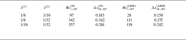
enhances sorting purity and reduces the necessary channel length, thereby improving efficiency. This is summarised in table 1, where superscripts (th) and (LBM) refer to predictions from theory and 3-D LBM simulations, respectively. Despite some quantitative differences, both methods confirm the existence of an intermediate
 ${\textit{Re}}_c$
that optimises
 $\Delta s$
.
The optimal Reynolds number
 ${\textit{Re}}_{c,opt}$
used to separate two filaments with different confinement ratios
 $\lambda ^{(1)}$
and
 $\lambda ^{(2)}$
, and the corresponding maximal separation
 $\Delta s_{eq}$
.

For mixtures of spheres and slender filaments, maximum separation is achieved at the highest laminar
 ${\textit{Re}}_c$
. At high
 ${\textit{Re}}_c$
, spheres migrate toward the wall, while filaments shift toward the centreline, increasing
 $\Delta s$
monotonically. This enables high-throughput, high-purity sorting and shortens entrance lengths (Matas et al. Reference Matas, Morris and Guazzelli2004), making high-
 ${\textit{Re}}_c$
operation especially advantageous.
This study focuses on filaments with aspect ratio
 $\kappa = 64$
due to field-of-view constraints. A broader investigation across the
 $(\lambda , \kappa )$
parameter space remains a valuable direction for future research.
We believe that the tendency of highly slender filaments to migrate toward the channel centreline at large
 ${\textit{Re}}_c$
mainly originates from the corrections of
 ${\textit{Re}}_G$
to the filament rotational dynamics. This effect is negligible for nearly spherical particles, where anisotropy is weak. However, when the focus is broadened to oblate particles with
 $\kappa \lt 0.14$
, and even to infinitely thin disks as
 $\kappa \to 0$
, similar effects to those described in this study re-emerge.
For oblate particles with
 $0.14\lt \kappa \lt 1$
, the log-rolling mode is the only stable orientation at finite fluid inertia (Dabade, Marath & Subramanian Reference Dabade, Marath and Subramanian2016). Consequently, such particles exhibit inertial migration characteristics similar to spheres, i.e. the equilibrium position shifts monotonically toward the wall with increasing
 ${\textit{Re}}_c$
. In contrast, for
 $\kappa \lt 0.14$
, both log rolling and tumbling become stable modes, and the selected mode depends on the initial orientation of the particle relative to the shear direction. In the log-rolling mode, the equilibrium position continues to move monotonically toward the wall as
 ${\textit{Re}}_c$
increases. By contrast, in the tumbling mode, finite
 ${\textit{Re}}_G$
corrections to the rotational dynamics begin to play a noticeable role, producing a tendency for the equilibrium position to shift toward the channel centreline. This trend strengthens as
 $\kappa \to 0$
.
Such behaviour suggests the possibility of orientation sorting of thin disks, determined by their initial orientation relative to the shear. For a suspension composed of identically sized thin disks, when passing through a laminar channel flow at sufficiently large
 ${\textit{Re}}_c$
, one could in principle infer the initial orientation distribution by statistically counting particles arriving at the two distinct equilibrium positions. Overall, particle shape plays a crucial role in determining equilibrium positions: when the aspect ratio is of order unity, equilibrium shifts monotonically toward the wall; when the aspect ratio tends to infinity (slender filaments) or to zero (thin disks in the tumbling mode), equilibrium tends instead to approach the channel centreline as
 ${\textit{Re}}_c$
increases.
4. Conclusions
This study presents a comprehensive investigation of the inertial migration of rigid filaments in planar Poiseuille flow, combining a quasi-analytical model with fully resolved 3-D numerical simulations. Using a singular perturbation method, we derive a migration-velocity expression that captures both instantaneous and period-averaged behaviour within a tumbling cycle. The model accounts for finite-size effects through the solid-phase inertia and a fluid-inertia-induced orientation dynamics. Complementing the theory, we implement a LBM-IBM framework to resolve flow–structure interactions in detail.
We first examine the migration of a filament held at a fixed orientation (
 $\phi = \pi /4$
), revealing a bathtub-shaped lateral migration-velocity profile. Both theory and simulations agree well, with minor discrepancies near the channel centre due to omitted shear-gradient effects in the theory. Unlike spherical particles, inclined filaments experience asymmetric inertial forces, leading to orientation-dependent attraction or repulsion near walls and multiple equilibrium positions.
To capture full dynamical behaviour, we develop a coupled system incorporating finite
 ${\textit{Re}}_G$
corrections to angular velocity. This model successfully predicts the filament’s complete tumbling and migration cycle, including oscillatory features in lateral and streamwise motion. At moderate
 ${\textit{Re}}_c = 24$
, theory and simulation match closely. At higher
 ${\textit{Re}}_c = 800$
, strong inertial effects cause temporary cessation of tumbling, followed by resumed rotation as
 ${\textit{Re}}_G$
decreases – behaviour captured for the first time. However, the theory breaks down when
 ${\textit{Re}}_{\!f} \gtrsim \mathcal{O}(1)$
, where RFT becomes invalid.
Our extended model outperforms previous theories by predicting the period-averaged migration velocity and quasi-equilibrium position with improved agreement over a wide range of Reynolds numbers and confinement ratios. Unlike earlier models, which predict near-wall equilibrium and monotonic wallward drift with increasing
 ${\textit{Re}}_c$
, our results show a centre-directed migration trend – matching simulations and experimental data. This highlights the importance of incorporating finite inertia and geometry into migration models.
Finally, we demonstrate that the quasi-equilibrium position strongly depends on the confinement ratio
 $\lambda$
for
 ${\textit{Re}}_c \in [10, 300]$
, offering potential for size-based sorting. Our findings provide a foundational framework for understanding filament migration and optimising microfluidic channel design for inertial focusing applications.
Acknowledgements
The authors would like to thank Professor Y, Liu and Mr J. Xiong for valuable discussions on topics related to this work. Calculations are performed at the Supercomputing Center of the University of Science and Technology of China.
Funding
This work was supported by the National Science Foundation of China (NSFC) (grant nos. 11972342).
Declaration of interests
The authors report no conflict of interest.
Appendix A
The incompressible Navier–Stokes equation is solved by the Multiple Relaxation Time lattice Boltzann method (Krüger et al. Reference Krüger, Kusumaatmaja, Kuzmin, Shardt, Silva and Viggen2017). The evolution equation is
 \begin{equation} \begin{aligned} &f_i\left (\boldsymbol{x}+\boldsymbol{e}_i \Delta t, t+\Delta t\right )-f_i(\boldsymbol{x}, t)=-\boldsymbol{M}^{-1} \boldsymbol{S} \boldsymbol{M}\big [f_i(\boldsymbol{x}, t)-f_i^{{eq}}(\boldsymbol{x}, t)\big ] \Delta t+F_i^{(v)}\Delta t \,, \end{aligned} \end{equation}
where
 $f_i(\boldsymbol{x},t)$
is the distribution function for velocity
 $\boldsymbol{e}_i$
at position
 $\boldsymbol{x}$
and time
 $t$
,
 $F_i^{(v)}$
is the forcing term,
 $\boldsymbol{M}$
is the transformation matrix and
 $\boldsymbol{S}$
is the relaxation matrix. The macroscopic variables can be calculated from
 \begin{equation} \rho =\sum _i f_i \,, \quad \quad \rho \boldsymbol{u}=\sum _i \boldsymbol{e}_i f_i+\frac {1}{2} \boldsymbol{f} \Delta t \,, \quad \quad p=c_s^2 \rho \,. \end{equation}
In 3-D LBM simulations, a velocity model referred to as Dimensions 3 Quantities 19 is adopted, characterised by 19 discrete velocities
 \begin{equation} \boldsymbol{e}_\alpha =\left \{\begin{array}{lr} (0,0,0) c, & \alpha =0 \\ ( \pm 1,0,0) c,(0, \pm 1,0) c,(0,0, \pm 1) c, & \alpha =1-6 \\ ( \pm 1, \pm 1,0) c,( \pm 1,0, \pm 1) c,(0, \pm 1, \pm 1) c, & \alpha =7-18 , \end{array}\right . \end{equation}
and their corresponding weighting coefficients
 \begin{equation} w_\alpha =\left \{\begin{array}{lr} 1/3, & \alpha =0 \\ 1/18, & \alpha =1-6 \\ 1/36, & \alpha =7-18 . \end{array}\right . \end{equation}
Here,
 $c$
represents the lattice velocity, while
 $c_s=c/\sqrt {3}$
denotes the lattice speed of sound.
The fluid–solid interaction is coupled through the IBM (Wu & Aidun Reference Wu and Aidun2010; Do-Quang et al. Reference Do-Quang, Amberg, Brethouwer and Johansson2014). In the IBM, the fluid force acting on the Lagrangian point,
 $\boldsymbol{F}^{(\textit{IB})}$
denoting the forces calculated at these ghost points (the grey circles in figure 10). Here,
 $\boldsymbol{r}$
signifies the position vector from the Lagrangian point to the respective ghost points, and
 $|\boldsymbol{r}|=\epsilon /2$
. The external force and torque at the
 $i$
th solid node (the yellow pentagrams in figure 10) is given by
 \begin{equation} \begin{aligned} &\boldsymbol{F}^s_i=\sum _{j=1}^4\boldsymbol{F}^{(\textit{IB})}_{\textit{ij}}.\\ &\boldsymbol{M}^s_i=\sum _{j=1}^4\boldsymbol{r_{\textit{ij}}}\times \boldsymbol{F}^{(\textit{IB})}_{\textit{ij}} \quad {\textrm on} \quad i\neq 1,(i)\textrm{max}. \end{aligned} \end{equation}
Subscript
 $i$
represents the number of solid nodes uniformly distributed along the axis of the filament, and subscript
 $j$
represents the ghost point number. For example,
 $r_{\textit{ij}}$
refers to the vector that points from the
 $i$
th solid node to its corresponding
 $j$
th ghost point. Here
 $\boldsymbol{F}^{(\textit{IB})}_{\textit{ij}}$
can be calculated by the penalty scheme (Goldstein, Handler & Sirovich Reference Goldstein, Handler and Sirovich1993)
 \begin{equation} \begin{aligned} \boldsymbol{F}^{(\textit{IB})}_{\textit{ij}}=\alpha \int _0^t\big [\boldsymbol{V}^f\big (\boldsymbol{X}_{\textit{ij}}, t^{\prime }\big )-\boldsymbol{V}^s\big(\boldsymbol{X}_{\textit{ij}}, t^{\prime }\big)\big ]\,\textrm{d} t^{\prime } +\beta \big[\boldsymbol{V}^f(\boldsymbol{X}_{\textit{ij}}, t)-\boldsymbol{V}^s(\boldsymbol{X}_{\textit{ij}}, t)\big ], \end{aligned} \end{equation}
where
 $\alpha$
and
 $\beta$
are parameters selected based on the previous studies (Xu et al. Reference Xu, Liu, Liu, Xiong and Huang2022). Here,
 $\boldsymbol{V}^s(\boldsymbol{X}_{\textit{ij}}, t)= {\partial \boldsymbol{X}_{\textit{ij}}}/{\partial t}$
is the velocity of the filament at the ghost points and
 $V_{\!f}$
is the fluid velocity at the position
 $ \boldsymbol{X}_{\textit{ij}}$
obtained by interpolation. The interpolation can be written as
 \begin{equation} \boldsymbol{V}^f(\boldsymbol{X}_{\textit{ij}}, t)=\int _{\varOmega } \boldsymbol{v}(\boldsymbol{x}, t) \mathcal{D}(\boldsymbol{x}-\boldsymbol{X}_{\textit{ij}}) \textrm{d} \boldsymbol{x}, \end{equation}
where
 $\mathcal{D}$
is the Dirac delta function and the subscript
 $\varOmega$
denotes the whole computational domain. Subsequently, the volume force on the Euler grid (the force acting on fluid points) can be obtained
 \begin{equation} \boldsymbol{F}^{(v)} (\boldsymbol{x}, t)=-\int _{\partial V_{\!f}} F^{(\textit{IB})}(\boldsymbol{X}_{\textit{ij}}, t) \mathcal{D}(\boldsymbol{x}-\boldsymbol{X}_{\textit{ij}}) \textrm{d} s. \end{equation}
A segment of the filament mesh: grey circles indicate Immersed Boundary (IB) ghost points; yellow pentagrams denote uniformly distributed solid nodes along the filament axis.

To avoid the issue of pseudo-oscillation associated with the weak fluid–structure coupling problem, we have adopted a
 $C^2$
continuous delta function Yang et al. (Reference Yang, Zhang, Li and He2009)
 \begin{equation} \mathcal{D}(r) = \left \{ \begin{array}{rcl} &\begin{aligned} \frac {3}{8}+\frac {\pi }{32}-\frac {r^2}{4}, \end{aligned} & |r| \leqslant 0.5 \\ &\begin{aligned} \frac {1}{4}+\frac {1-|r|}{8} \sqrt {-2+8|r|-4 r^2}-\frac {1}{8} \arcsin (\sqrt {2}(|r|-1)), \end{aligned} & 0.5 \leqslant |r| \leqslant 1.5, \\ &\begin{aligned} \frac {17}{16}-\frac {\pi }{64}-\frac {3|r|}{4}+\frac {r^2}{8}+\frac {|r|-2}{16} \sqrt {-14+16|r|-4 r^2} \end{aligned} & \\ &\begin{aligned} +\frac {1}{16} \arcsin (\sqrt {2}(|r|-2)), \end{aligned} & 1.5 \leqslant |r| \leqslant 2.5, \\ &\begin{aligned} 0 \end{aligned} & 2.5 \leqslant |r| . \end{array} \right . \end{equation}
The persistent pseudo-oscillation problem, prevalent due to the small linear density ratio of the filament, is thereby tackled. In order to obtain accurate and stable solutions, we have introduced predictors to determine the provisional velocity and position of the fluid–structure interface at each time step (Kim, Lee & Choi Reference Kim, Lee and Choi2018).
To maintain the condition of zero torque at both ends of the filament, the torque at the free end nodes should be set as
 $\boldsymbol{M}^s_i=-\sum _{j=1}^4\boldsymbol{r_{\textit{ij}}}\times \boldsymbol{F}_{\textit{ij}}\quad {\textrm on} \quad i=1,i_{\textit {max}}$
(Banaei, Rosti & Brandt Reference Banaei, Rosti and Brandt2020). Although torque is a small quantity (
 $O(\kappa ^{-2})$
) for slender filaments, when the filament is aligned with the flow direction, this torque becomes the sole driving factor for filament rotation. Therefore, accurately assessing torque is crucial.
The motion of filament is governed by Newton’s laws and the Euler equations of dynamics
 \begin{equation} \begin{gathered} M \frac {{\textrm d} \boldsymbol{u}_{\!f}}{{\textrm d} t}=\boldsymbol{F}_{\!f} ,\\ I \frac {{\textrm d} \boldsymbol{\omega }_{\!f}}{{\textrm d} t}+\boldsymbol{\omega }_{\!f} \times \left [I \boldsymbol{\cdot }\boldsymbol{\omega }_{\!f}\right ]=T_{\!f}. \end{gathered} \end{equation}
Here,
 $\boldsymbol{F}_{\!f}$
and
 $\boldsymbol{T}_{\!f}$
represent the force and torque acting on the filament, respectively, while
 $ \boldsymbol{U}_p$
and
 $ \boldsymbol{\omega }_p$
denote the translational velocity and angular velocity of the filament. Additionally,
 $M$
and
 $I$
are the filament’s mass and moment of inertia tensor, respectively. Direct numerical solutions of the aforementioned Euler kinematic equations face singularity issues. To overcome this, the quaternion method proposed in prior studies is adopted (Qi & Luo Reference Qi and Luo2003). To validate our numerical method, in a computational domain that is sufficiently large, we simulated the cases of a rigid filament tumbling in shear flow at
 ${\textit{Re}}_G=0.1$
. In this case, the spatial resolution is also set at
 $\Delta s=1/64$
, with a time resolution of
 $\Delta t=2\times 10^{-4}$
. As shown in figure 11(a), the rigid filament is initially aligned with the flow direction and subsequently undergoes periodic tumbling within the velocity-gradient plane due to the fluid motion. Figure 11(b) shows that our results agree well with the numerical, experimental and theoretical data (Trevelyan & Mason Reference Trevelyan and Mason1951; Cox Reference Cox1971; Wu & Aidun Reference Wu and Aidun2010) for the non-dimensional tumbling period
 $T_p$
as a function of
 $r_p$
.
(a) Rigid filament tumbling in shear flow (plotted at equal time intervals), (b) tumbling period of a rigid filament in shear flow.

Appendix B
If the global self-hydrodynamic interactions are neglected and the shear Reynolds number is much smaller than 1, the fluid force distribution acting on the filament at position
 $\xi$
can be calculated using the so-called RFT
 \begin{equation} \begin{aligned} \boldsymbol{f}_{\!f}(\xi )=&-\lambda _1\Delta \boldsymbol{u}_{\mathop {//}}(\xi )-\lambda _2\Delta \boldsymbol{u}_\perp (\xi ). \end{aligned} \end{equation}
Here,
 $\Delta \boldsymbol{u}(\xi )=\boldsymbol{u}_{f}(\xi )-\boldsymbol{u}_{bg}(\xi )$
represents the velocity difference between the filament velocity at position
 $\xi$
and the undisturbed background flow. The subscripts
 $_{//}$
and
 $_\perp$
correspond to the components parallel and perpendicular to the filament axis within the vorticity plane, respectively. Where
 \begin{equation} \begin{aligned} \boldsymbol{u}_{bg}(\xi )&=4U_m(d+\xi \cos \phi )(H-d-\xi \cos \phi )/H^2\boldsymbol{e}_1, \end{aligned} \end{equation}
and
 \begin{equation} \begin{aligned} \boldsymbol{u}_{\!f}(\xi )&=(u_{f1}+\dot {\phi }\xi \cos \phi )\boldsymbol{e}_1+(u_{f2}-\dot {\phi }\xi \sin \phi )\boldsymbol{e}_2. \end{aligned} \end{equation}
Simple integration over the coordinate
 $\xi$
yields the expressions for the force monopole
 \begin{equation} \begin{aligned} \boldsymbol{F}_{\!f}&=\int _{-a}^{a}\boldsymbol{f}_{\!f}(\xi ){\textrm d}\xi \\ &=\left[C_1(4U_md(H-d)/H^2-u_{f1})a-C_2u_{f2}a+C_1\frac {1}{3}a^3\cos ^2\phi \right]\boldsymbol{e}_1\\ &\quad +\left[C_2(4U_md(H-d)/H^2-u_{f1})a-C_3u_{f2}a+C_2\frac {1}{3}a^3\cos ^2\phi \right]\boldsymbol{e}_3, \end{aligned} \end{equation}
and force dipole
 \begin{equation} \begin{aligned} \boldsymbol{D}_{\!f} &=\int _{-a}^{a}\xi \boldsymbol{f}_{\!f}(\xi )\boldsymbol{e}_{\mathop {//}}{\textrm d}\xi \\ &=\begin{bmatrix} -\frac {a^3\sin (2\phi )}{3}(\lambda _2\dot {\phi }+C_4)&0&-\frac {2a^3\sin ^2\phi }{3}(\lambda _2\dot {\phi }+C_4) \\ 0 & 0&0 \\ \frac {2a^3\sin \phi }{3}(\lambda _2\dot {\phi }\sin \phi -C_5\cos \phi ) & 0& \frac {2a^3\cos \phi }{3}(\lambda _2\dot {\phi }\sin \phi -C_5\cos \phi ) \end{bmatrix}\!, \end{aligned} \end{equation}
with the associated coefficients summarised in table 2. By isolating the antisymmetric part in (B5), the torque acting on the filament can be obtained
 \begin{equation} \begin{aligned} \boldsymbol{T}_{f}^{(0)}=\frac {2\lambda _2a^3}{3}(\dot {\phi }-4U_m(1-2d)/H^2\cos ^2{\phi })\boldsymbol{e}_2. \end{aligned} \end{equation}
Which provides a good approximation for
 $ \phi \neq 0$
; however, when
 $ \phi = 0$
, the O
 $(\kappa ^{-2})$
distributed torque on the filament must be considered. Specifically, we replace the second term on the right-hand side with the result from Chwang (Reference Chwang1975)
 \begin{equation} \boldsymbol{T}_{\!f}=\frac {2\lambda _2a^3}{3}\dot {\phi }-\frac {128\pi \mu e^3 a_1^3U_m(1-2d)/H^2(1-e^2\sin ^2\phi )}{3\left [-2e+(1+e^2)\log (\frac {1+e}{1-e})\right ]}. \end{equation}
Here,
 $ e = \sqrt {1 - ( \kappa _e )^{-2}}$
denotes the eccentricity, and
 $ \kappa _e = 1.24 \, \kappa / \sqrt { \ln \kappa }$
is the equivalent aspect ratio (Cox Reference Cox1971).
Values of coefficient
 $C_\alpha$
and
 $\lambda _\alpha$
.

Appendix C
The numerical solution of (3.16) is described in the Appendix of Asmolov (Reference Asmolov1999) and in appendix D of Anand & Subramanian (Reference Anand and Subramanian2023). Here, we emphasise the use of an adaptive Lobatto Runge–Kutta method for solving the boundary-value problem, which enhances both efficiency and accuracy compared with previous approaches. This appendix provides an outline of the algorithm framework and the error evaluation method. Additionally, all symbol definitions in this section follow the conventions established in Wanner & Hairer (Reference Wanner and Hairer1996). The s-stage implicit Runge–Kutta method
 \begin{equation} \begin{aligned} & g_i=y_0+h \sum _{j=1}^s a_{i j} f\left (x_0+c_j h, g_j\right ) \quad i=1, \ldots , s \\ & y_1=y_0+h \sum _{j=1}^s b_j f\left (x_0+c_j h, g_j\right )\!, \end{aligned} \end{equation}
where the coefficients
 $a_{\textit{ij}}$
,
 $b_j$
,
 $c_j$
characterising the five-stage Lobatto IIIC
 $^*$
method are displayed below in the form of a table called a Butcher-tableau (Butcher Reference Butcher2016)
 \begin{align} \begin{array}{c|ccccc} 0 & \frac {1}{20} & -\frac {7}{60} & \frac {2}{15} & -\frac {7}{60} & \frac {1}{20} \\[10pt] \frac {1}{2} - \frac {\sqrt {21}}{14} & \frac {1}{20} & \frac {29}{180} & \frac {47 - 15\sqrt {21}}{315} & \frac {203 - 30\sqrt {21}}{1260} & -\frac {3}{140} \\[10pt] \frac {1}{2} & \frac {1}{20} & \frac {329 + 105\sqrt {21}}{2880} & \frac {73}{360} & \frac {329 - 105\sqrt {21}}{2880} & \frac {3}{160} \\[10pt] \frac {1}{2} + \frac {\sqrt {21}}{14} & \frac {1}{20} & \frac {203 + 30\sqrt {21}}{1260} & \frac {47 + 15\sqrt {21}}{315} & \frac {29}{180} & -\frac {3}{140} \\[10pt] 1 & \frac {1}{20} & \frac {49}{180} & \frac {16}{45} & \frac {49}{180} & \frac {1}{20} \\[4pt] \hline\\[-8pt] C_{s=5} & \frac {1}{20} & \frac {49}{180} & \frac {16}{45} & \frac {49}{180} & \frac {1}{20} \end{array} \end{align}
Whether the calculation converges with sufficient accuracy will be evaluated using residuals (Russell & Christiansen Reference Russell and Christiansen1978)
 \begin{equation} r(x)=\frac {y^{(6)}\left (x_{i+1 / 2}\right )}{5!} \prod _{j=1}^{5}\left (x-t_{i j}\right )+O\big (h^{6}\big ). \end{equation}
In all the calculations involving (3.16) in this paper, it is required that the norm of all components in residual vector be less than
 $10^{-6}$
. A knot selection scheme which the residuals are evenly distributed on the knot has been implemented by requiring (Russell & Christiansen Reference Russell and Christiansen1978)
 \begin{equation} r(x_{i+1/2})h_i=\frac {1}{2^6 \, 5!} \max _{-1 \leqq x \leqq 1}\left |\int _{-1}^x \prod _{j=1}^{5}\left (t-t_{j}\right ) {\textrm d} t\right |(1+O(h)). \end{equation}
Such a method can be interpreted as perturbed collocation methods (Nørsett & Wanner Reference Nørsett and Wanner1981), and
 $t_j$
is the collocation points in
 $[-1,1]$
.
(a) Numerical solution of the migration velocity as a function of the number of grid points. (b) Normalised grid-point distribution obtained using the implicit Runge–Kutta method. PDF is Probability Density Function.

To assess the numerical efficiency of the implicit Runge–Kutta method, we compute the migration velocity for
 ${\textit{Re}}=100$
,
 $k_x=50$
,
 $k_y=50$
,
 $\phi =pi/4$
and
 $s=0.655$
. The results are shown in figure 12(a). The grey line denotes the asymptotic prediction given by (3.23), which approaches
 $3.00611914\times 10^{-11}$
.
The orange triangles show results obtained using the orthonormalisation method following Asmolov (Reference Asmolov1999): the fourth-order explicit Runge–Kutta scheme is applied from both channel boundaries on a uniform grid, combined with Gram–Schmidt orthonormalisation to suppress exponential growth of numerical errors. The yellow squares correspond to the adaptive-step 5-stage Lobatto IIIC implicit Runge–Kutta method. For
 $N_{\textit{grid}}\in [200,,1.6\times 10^6]$
, both methods converge toward the same limiting solution as the grid is refined; however, the orthonormalisation method requires roughly three orders of magnitude more grid points to reach comparable accuracy.
We note that figure 12(a) compares the numerical results only against the asymptotic prediction, which is not the exact analytical solution; at finite
 $k$
, an
 $O(k^{-1})$
relative error remains. For example, at
 $N_{\textit{grid}} = 10^4$
, the relative deviation of the implicit Runge–Kutta result from the asymptotic prediction is already
 $\lt 10^{-4}$
, whereas the orthonormalisation method still shows a visibly larger deviation even at
 $N_{\textit{grid}} = 10^6$
. This confirms that the implicit Runge–Kutta method provides a substantially more efficient and robust means of solving the stiff boundary-value problem.
The pronounced difference in computational efficiency arises because the orthogonalisation method transforms the boundary-value problem into two initial-value problems, followed by the solution of a linear algebraic system, whereas the present implicit Runge–Kutta method addresses the boundary-value problem directly and, by adopting an adaptive step-size strategy, achieves a nearly uniform distribution of residuals over the grid points. As shown in figure 12(b), this leads to a higher grid-point density near the jump condition, while the mesh remains sparse in most other regions. By contrast, the orthogonalisation method for comparison uses a uniform grid.
It should be noted that the total computation time of the implicit Runge–Kutta method is sensitive to the choice of the initial guess. Specifically, we use a uniform grid with all components initialised to zero, and convergence from such a rough initial guess typically requires
 $\mathcal{O}(10^2)$
function evaluations per grid point. Consequently, although the implicit Runge–Kutta method requires far fewer grid points than the orthogonalisation method, the overall computation time is reduced by only approximately one order of magnitude.
Appendix D
In this appendix, we derive the asymptotic solution of the governing equation in the limit
 $k \to \infty$
. The operational framework employed here is consistent with the fundamental principles set out in appendix D of Hogg (Reference Hogg1994). Let
 $k_1 = k \cos \theta$
and
 $k_2 = k \sin \theta$
, where
 $\theta =\arccos (k_1/k)$
. Equation (3.12), together with the no-slip boundary conditions at the upper and lower walls, can then be written as
 \begin{align} \frac {\textrm{d}^4\widetilde {W}_3}{\textrm{d}Z^4}&-2k^2\frac {\textrm{d}^2\widetilde {W}_3}{\textrm{d}Z^2}+k^4\widetilde {W}_3 \nonumber\\ &-ik\cos \theta \big(\gamma Z-4{\textit{Re}}_c^{-1/2}Z^2\big)\left (\frac {\textrm{d}^2\widetilde {W}_3}{\textrm{d}Z^2}-k^2\widetilde {W}_3\right )-ik\cos \theta 8{\textit{Re}}_c^{-1/2}\widetilde {W}_3=0, \end{align}
 \begin{align} &\qquad\qquad\quad \widetilde {W}_3=\frac {\textrm{d} \widetilde {W}_3}{\textrm{ d} Z}=0, \quad Z=Z^{+}, Z^{-} ; \quad Z^{+}-Z^{-}=R_c^{\frac {1}{2}} .\end{align}
We introduce
 $\varepsilon =1/k$
as a small parameter and seek an asymptotic solution for
 $\widetilde {W}_3$
in the regime
 $0\lt \varepsilon \ll 1$
. Next, we introduce a rescaled variable
 $\eta =Z/{\varepsilon }$
and set
 $\mathscr{W}(\eta ) = {\widetilde {W}}_3(Z)$
. The equation to be solved can then be written as
 \begin{equation} \frac {\textrm{d}^4\mathscr{W}}{\textrm{d}\eta ^4}-2\frac {\textrm{d}^2\mathscr{W}}{\textrm{d}\eta ^2}+\mathscr{W}\!=i\varepsilon \cos \theta (\gamma \varepsilon \eta -4{\textit{Re}}_c^{-1/2}\varepsilon ^2\eta ^2)\!\left (\!\frac {\textrm{d}^2\mathscr{W}}{\textrm{d}\eta ^2}-\mathscr{W}\!\right )\!+i\varepsilon ^3\!\cos \theta 8{\textit{Re}}_c^{-1/2}\mathscr{W}\!. \end{equation}
We propose the following asymptotic expansion:
 \begin{equation} \begin{aligned} \mathscr{W}=\mathscr{W}_0+\varepsilon \mathscr{W}_1+\varepsilon ^2\mathscr{W}_2+\varepsilon ^3\mathscr{W}_3+O(\varepsilon ^3). \end{aligned} \end{equation}
We first examine the zeroth-order term, which must satisfy the governing equation together with the jump condition at the origin
 \begin{equation} \begin{aligned} \frac {\textrm{d}^4\mathscr{W}_0}{\textrm{d}\eta ^4}-2\frac {\textrm{d}^2\mathscr{W}_0}{\textrm{d}\eta ^2}+\mathscr{W}_0=0, \end{aligned} \end{equation}
 \begin{equation} \begin{aligned} &\left [ \frac {{\textrm d}\mathscr{W}_0}{{\textrm d}\eta }\right ]=-\frac {{\textit{Re}}_c^{-1/2}}{4\pi ^2}i\cos \theta D_{f13},\\ &\left [ \frac {\textrm{d}^2\mathscr{W}_0}{{\textrm d}\eta ^2}\right ]=-\frac {{\textit{Re}}_c^{-1/2}}{4\pi ^2}\big(-\cos ^2 \theta D_{f11}+D_{f33}\big),\\ &\left [ \frac {\textrm{d}^3\mathscr{W}_0}{{\textrm d}\eta ^3}\right ]=-\frac {{\textit{Re}}_c^{-1/2}}{4\pi ^2}i\cos \theta \big(2 D_{f13}+ D_{f31}\big).\\ \end{aligned} \end{equation}
As the right-hand side of (4.7) is asymptotically smaller than the left-hand side by at least
 $O(\varepsilon ^2)$
, we may assume that solutions at each order of
 $\mathscr{W}_n$
can be expressed as linear combinations of exponential basis
 $e^{\pm \eta }$
and
 $\eta e^{\pm \eta }$
. It is noted that the exponentially growing solutions contribute to the migration velocity only at order
 $O(e^{-2\eta ^{\pm }})$
, becoming significant only when
 $Z^\pm =O(\varepsilon )$
, which corresponds to the case where the filament centre is very close to one of the channel walls. Therefore, in the following discussion we retain only the exponentially decaying basis
 \begin{equation} \begin{aligned} &\mathscr{W}_0^-=A_{\mathscr{W}_0}^-e^\eta +B_{\mathscr{W}_0}^-\eta e^\eta ,\quad \mathscr{W}_0^+=A_{\mathscr{W}_0}^+e^{-\eta }+B_{\mathscr{W}_0}^+\eta e^{-\eta } .\end{aligned} \end{equation}
In this expression, the coefficients
 $A_{\mathscr{W}_0}^\pm =$
and
 $B_{\mathscr{W}_0}^\pm$
are specified by enforcing the no-slip condition at the origin, as well as at the upper and lower boundaries. We then obtain the zeroth-order migration velocity
 \begin{equation} \begin{aligned} &\mathscr{W}_0|_{\eta =0}=A_{\mathscr{W}_0}^-=\frac {{\textit{Re}}_c^{-1/2}}{16\pi ^2}i\cos \theta (D_{f13} - D_{f31}). \end{aligned} \end{equation}
It is found that the first-order contribution is purely imaginary. A straightforward repetition of the preceding procedure yields
 \begin{equation} \begin{aligned} &\mathscr{W}_1|_{\eta =0}=0,\\ &\mathscr{W}_2|_{\eta =0}=\frac {{\textit{Re}}_c^{-1/2}}{32\pi ^2}i\cos \theta \gamma (\cos ^2\theta D_{f11} - D_{f33}),\\ &\mathscr{W}_3|_{\eta =0}=\frac {3{\textit{Re}}_c^{-1}}{32\pi ^2}\cos ^2\theta (D_{f13} + 5D_{f31}). \end{aligned} \end{equation}
Accordingly, the cumulative contribution to the migration velocity from the wavenumber interval
 $k \in (K_m, \infty )$
may be estimated as
 \begin{equation} \mathscr{W}^{({far field})}= {{\textit{Re}}}\left [\int _{0}^{2\pi } \int _{K_m}^{\infty }\frac {3(D_{f13}+5 D_{f31})\cos ^2\theta }{32\pi ^2 {\textit{Re}}_c k^3}\textrm{ d} k \textrm{ d} \theta \right ]= \frac {3(D_{f13}+5 D_{f31})}{64\pi {\textit{Re}}_c K_m^2}. \end{equation}
Appendix E
The theoretical model presented in this work predicts that the lateral migration velocity vanishes when the filament centroid lies exactly on the channel centreline. However, as shown in figure 3(c), the LBM results clearly demonstrate a non-zero migration velocity at the centreline. Moreover, under the scaling
 $\epsilon ^{-3}{\textit{Re}}^{1/2}$
used for the vertical axis in figure 3(c), the centreline migration velocity appears to increase as
 $\lambda$
decreases.
Centreline lateral migration velocity
 $w_3|_{s=0.5}$
of a filament inclined at
 $\phi = \pi /4$
for various values of
 $\lambda$
. (a) Red hollow markers indicate LBM simulation results, while grey dashed lines show corresponding linear fits. (b)The coloured markers represent the LBM simulation results, while the grey solid line denotes a quadratic fit to the data.

Understanding this discrepancy between theory and simulation at this special location helps clarify the limitations of the theoretical model. To better illustrate the trend, we replot the LBM results in figure 13(a) using red hollow markers, along with a grey dashed line representing a linear fit, which indicates a strict proportionality between
 $1/\lambda$
and
 $-w_3|_{s=0.5}\epsilon ^{-3}{\textit{Re}}^{1/2}$
. This may lead to a misunderstanding: that a smaller
 $\lambda$
, which corresponds to a filament located further from both walls and experiencing a smaller shear gradient, results in a larger migration velocity.
This apparent contradiction arises because both figures 3(c) and 13(a) adopt a vertical-axis scaling
 $\epsilon ^{-3}{\textit{Re}}^{1/2}$
based on the theoretical model, which accounts only for the contribution from the local shear rate. It does not include the contribution from the disturbance flow induced by the interaction between the filament and the shear gradient – terms associated with quadratic part of the ambient flow. At the channel centreline, the shear rate vanishes, while the shear gradient remains finite and constant, making the latter the dominant contributor to the migration velocity at leading order.
To address this, we replot the relationship between
 $\lambda$
and
 $w_3|_{s=0.5}$
in figure 13(b). It is found that, over a relatively wide range of Reynolds numbers
 ${\textit{Re}}_c\in [40,1280]$
, the migration velocity is insensitive to
 ${\textit{Re}}_c$
. A fitting analysis shows that all data points collapse onto the grey dashed curve corresponding to the quadratic relation
 $w_3|_{s=0.5}=-0.036\lambda ^2$
.
These results highlight a primary limitation of the present theoretical model – namely, its omission of the quadrupolar contribution arising from the interaction between the filament and the secondary flow induced by the shear gradient.
Appendix F
Einarsson et al. (Reference Einarsson, Candelier, Lundell, Angilella and Mehlig2015) derived approximate angular equations for neutrally buoyant ellipsoidal spheres (
 $St={\textit{Re}}_G$
) in unbounded shear flows
 \begin{equation} \begin{aligned} \dot {\boldsymbol{p}}= & \mathbb{O}^{\infty } \boldsymbol{p}+\varLambda \left [\mathbb{S}^{\infty } \boldsymbol{p}-\left (\boldsymbol{p} \boldsymbol{\cdot }\mathbb{S}^{\infty } \boldsymbol{p}\right ) \boldsymbol{p}\right ]+\beta _1\left (\boldsymbol{p} \boldsymbol{\cdot }\mathbb{S}^{\infty } \boldsymbol{p}\right ) \mathbb{P}_{\perp } \mathbb{S}^{\infty } \boldsymbol{p} \\ & +\beta _2\left (\boldsymbol{p} \boldsymbol{\cdot }\mathbb{S}^{\infty } \boldsymbol{p}\right ) \mathbb{O}^{\infty } \boldsymbol{p}+\beta _3 \mathbb{P}_{\perp } \mathbb{O}^{\infty } \mathbb{S}^{\infty } \boldsymbol{p}+\beta _4 \mathbb{P}_{\perp } \mathbb{S}^{\infty } \mathbb{S}^{\infty } \boldsymbol{p} . \end{aligned} \end{equation}
where
 $\varLambda = (\kappa ^2-1 ) / (\kappa ^2+1 )$
, and
 $\mathbb{P}_{\perp }(\boldsymbol{x}) = \boldsymbol{x} - (\boldsymbol{p} \boldsymbol{\cdot }\boldsymbol{x}) \boldsymbol{p}$
is an operator that projects components in the
 $\boldsymbol{p}$
-direction. Here,
 $\mathbb{S}^{\infty }=(\mathbb{A}+\mathbb{A}^T)/2$
and
 $\mathbb{O}^{\infty }=(\mathbb{A}-\mathbb{A}^T)/2$
denote the symmetric and antisymmetric parts of the gradient tensor
 $\mathbb{A}_{\textit{ij}}=\delta _{i1}\delta _{j2}$
, respectively. The last four terms on the right-hand side include the coefficient
 $\beta _\alpha ={\textit{Re}}_Gb_\alpha$
to achieve O
 $({\textit{Re}}_G)$
corrections, where (Rosén et al. Reference Rosén, Einarsson, Nordmark, Aidun, Lundell and Mehlig2015)
 \begin{equation} \begin{aligned} b_1 =& \frac {7}{15(2 \ln \kappa -3+\ln 4)}+\frac {-197 \ln 2 \kappa +92 \ln \kappa \ln 4 \kappa +106+92(\ln 2)^2}{15 \kappa ^2(2 \ln \kappa -3+\ln 4)^2} ,\\ b_2 =& \frac {1}{5(2 \ln \kappa -3+\ln 4)}+\frac {(\ln \kappa -1+\ln 2)(8 \ln 2 \kappa -7)}{5 \kappa ^2(2 \ln \kappa -3+\ln 4)^2} ,\\ b_3 =& -\frac {4}{5 \kappa ^2}, \\ b_4 =& \frac {4}{15 \kappa ^2} .\end{aligned} \end{equation}
More simply, for a filament moving within the shear-gradient plane, the Reynolds number correction to the azimuthal angle is given by
 \begin{equation} \begin{aligned} \dot {\phi }^{\textit(corr)}=\dot {\phi }^{(\textit{Einarsson})}-\dot {\phi }^{(\textit{Jeffery})}=\frac {1}{2}\left [\beta _1 \cos 2 \phi +\beta _2+\beta _3\right ]\sin \phi \cos \phi. \end{aligned} \end{equation}