1.0 Introduction
The research for specific angle constraints involves forcing the desired terminal engagement geometries without relaxing the requirement of achieving ideal miss distance [Reference Zarchan1]. Depending on the practical application, controlling the terminal angle is important [Reference Wang, Tang and Guo2] and may introduce the following advantages: attacking the weak part of the target, increasing the power of warhead to improve the effectiveness, avoiding enemy directional defense and reducing additional damage.
Numerous studies on impact angle constraint problems have been conducted. Previous works focusing on the problem of impact angle control may be investigated mainly under two categories: optimal control theory-based and proportional navigation-based methods. Literature [Reference Kim and Grider3] is probably the first study related to impact angle problems, in which a suboptimal guidance law is derived for a reentry vehicle. Literature [Reference Bryson and Ho4] provides an optimal solution for an ordinary intersection problem by minimising the performance index for terminal position and velocity constraints. The solution can be used for impact angle constraint problems if the intersection procedure is defined as the expected collision process. The performance index is selected as an opposite time-varying weighting function in literature [Reference Cho5] for an optimal impact angle constraint guidance law. A highly usual guidance law to achieve the expected impact angle is accomplished by adjusting the gain of the weighting functions. In literature [Reference Ryoo, Cho and Tahk6], arbitrary order missile dynamics are considered in the optimal impact angle constraint problems, thus providing a generalised formulation. In literature [Reference Qian, Yang and Geng7], the state-dependent Riccati equation method, which is widely used in various kinds of nonlinear control issues, is applied to cope with the impact angle constraint problems. In literature [Reference Lee, Kim and Tahk8], a linear time-varying guidance law is addressed using the inverse problem in optimal control theory to attain expected impact angle and small miss distance.
Studies based on optimal control theory are available as above. Meanwhile, proportional navigation (PN) is widely used to solve impact angle constraint problems. In literature [Reference Kim, Lee and Han9], a time-varying bias term called the biased proportional navigation guidance (BPNG) law is added to the traditional PN, and this bias term achieves impact angle constraints. In literature [Reference Ratnoo and Ghose10], the guidance law comprises PN coefficient with two phases: one for generating an orientation trajectory to cover all impact angles from 0 to −π with navigation gain
 $N \lt 2$
, and the other for attacking the stationary target at a desired impact angle with
 $N \ge 2$
. In literature [Reference Erer and Ozgoren11], two PN guidance laws based on the rotation of the relative velocity vector are presented, and the impact angle can be controlled through the bias term against a nonstationary target. In literature [Reference Erer, Tekin and Kemal12], the author utilises a bias term to enhance PN through an error signal, which is a function of pursuit angles, to accommodate the problem of impact angle control against a stationary target. In literature [Reference Zhang, Ma and Wu13], the constructed impact angle control guidance law is a BPNG law with large impact angle constraint, which is required in the development of time-to-go estimation procedure. The two-phase BPN in literature [Reference Erer, Tekin and Ozgoren14] utilises the unbiased and biased pure PN laws where the necessary analytical solutions are derived. The logic is based on switching action, where the navigation gain and the bias are switched when proper conditions for the terminal phase are achieved. In literature [Reference Yang, Wang and Lin15], a time-varying BPNG law is designed by Yang et al. to achieve the terminal angle constraints; this law has two time-varying bias terms. Considering the two-phase BPN and composite guidance law, Tekin and Erer [Reference Tekin and Erer16] propose the PN gain switched strategy, which can accomplish specific terminal angles; however, the look angle has an increase in flight process. Based on a two-stage PN guidance law, Ratnoo [Reference Ratnoo17] derives a closed-form solution for the choice of navigation gains for achieving all possible impact angles. In literature [Reference Park, Kwon and Kim18], a composite guidance scheme is presented considering the case of a non-manoeuvering moving target, which comprises a modified deviated pure pursuit with error feedback loop of look angle for initial guidance phases and PN with
 $N \ge 3$
for final guidance phases. Park et al. [Reference Park, Kim and Tahk19] deals with the problems of impact angle control against non-manoeuvering targets by using the guidance law comprising two time-varying biases and extending it to consider the command limit. Zhang et al. [Reference Zhang, Tang and Guo20] draws on the experience of PN gain switched strategy to extend the investigated case to a non-manoeuvering moving target to achieve terminal angle constraints.
While the aforementioned guidance strategies all adopt a two-phase method or an additional bias term to the traditional PN law, this study proposes a new method based on the research of the preceding literatures. Specific terminal angle constraints are accomplished only through a time-varying proportional navigation coefficient without phased or adding a bias term. The contributions of this study are as follows. (1) The monotonicity of look angles and accelerations with PN coefficient, which are the bases for the derivation of the proposed guidance law, are provided. (2) Different from literature [Reference Kim, Lee and Han9], the proposed method does not need to estimate time-to-go and give a switch strategy, as seen in literature [Reference Tekin and Erer16]; thus the method can be conveniently implemented in real missile model. (3) From the derivation of this study, the two-phase pure proportional navigation (PPN) in literature [Reference Tekin and Erer16] is a special case of the proposed method, which illustrates that the proposed approach generates a generalised guidance law that covers results in Ref. [Reference Tekin and Erer16].
The remainder of this paper is structured as follows. Section 2 establishes the equations of motion, and several fundamental conclusions are stated as bases. The proposed time-varying navigation coefficient is derived in Section 3 for specific terminal angle constraints. Section 4 presents representative results of the derived guidance law for several typical engagement scenarios with a few comparisons. Section 5 provides conclusions.
2.0 Problem statement
In Section 2.1, the kinematic equations are established in longitudinal plane for a stationary target, and then the state variables in 3D space are given. In Section 2.2, the relationship among look angles, accelerations and PN coefficients, which limits the selection of design parameters in Section 3, are obtained.
2.1 Engagement kinematics
Figure 1 displays the engagement between an offensive missile
 $M$
and a stationary target
 $T$
in longitudinal plane, where
 $r$
is the relative distance between the missile and the target. The velocity magnitude of the missile is
 ${V_M}$
, and the magnitude of its normal acceleration is
 ${a_{yc}}$
, which is perpendicular to the velocity vector.
 $\theta $
represents the flight path angle of the missile, and
 $q$
denotes the line-of-sight (LOS) angle. The angle between the velocity vector and the LOS is the look angle
 $\rho $
. All angles are positive in the counterclockwise direction.
Engagement geometry in longitudinal plane.

The relative kinematic equations between the missile and the stationary target are given respectively
 \begin{align}\dot r = - {V_M}\cos\!(\theta - q) = - {V_M}\cos \rho,r(0) = {r_0},\end{align}
 \begin{align}\dot q = - \frac{{{V_M}\sin\!({\theta - q})}}{r} = - \frac{{{V_M}\sin \rho }}{r}\,\,,\,\,\,\,\,q(0) = {q_0},\end{align}
where
 ${r_0}$
and
 $\,{q_0}\;$
are initial values of relative distance and LOS angle between the missile and the target, respectively. For convenience of explanation, assume
 ${V_M}$
is a constant firstly. However, the guidance law in Section 3 is unrelated to the velocity, that is to say, the impact angle constraints can be satisfied for variable speed, which will be validated in the simulation in Section 4.
Engagement geometry in 3D plane.

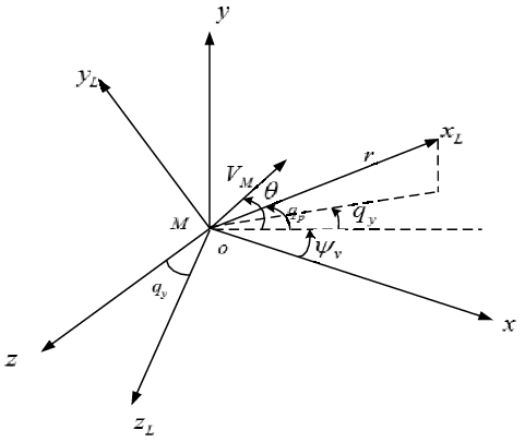
In a 3D guidance space, the relative motion between the missile and the target is exhibited in Fig. 2.
 $\,oxyz$
is the inertial reference coordinate system,
 $\,o{x_L}{y_L}{z_L}$
is the LOS coordinate system, and
 $M$
represents the missile. The magnitude of its acceleration in lateral plane is
 ${a_{zc}}$
.
 ${q_p}$
and
 $\,{q_y}$
are the LOS angles in longitudinal and lateral planes, respectively.
 ${\psi _v}$
represents the flight deflection angle of the missile. The look angle components in longitudinal and lateral planes are
 ${\rho _p}$
and
 ${\rho _y}$
, respectively. These components satisfy the equation below.
 \begin{align}{\rho _p} = \theta - {q_p},\end{align}
 \begin{align}{\rho _y} = {\psi _v} - {q_y}.\end{align}
2.2 Fundamental theories
The purpose of this part is to illustrate the influence of PN coefficient on look angles and accelerations. The design parameter in Section 3 should satisfy the limitation of PN coefficient in this part.
Taking kinematic equations in longitudinal plane as an example, the supplementary equation defining the relationship between the flight path angle and LOS angle is as follows:
 \begin{align}{\rho _p} = \theta - {q_p}.\end{align}
Acceding to the condition that the missile is guided by PPN, the guidance equation is
 \begin{align}{a_{yc}} = {N_p}{V_M}\,{\dot q_p}.\end{align}
Owing to
 \begin{align}\dot \theta = \frac{{{a_{yc}}}}{{{V_M}}},\end{align}
Equation (7) can be rewritten as follows:
 \begin{align}\dot \theta = {N_p}\,{\dot q_p}.\end{align}
Evidently, the flight path angular rate is proportional to the LOS angular rate, where
 ${N_p}$
is referred to as the scale coefficient or the navigation gain in longitudinal plane.
Differentiating Equation (5):
 \begin{align}{\dot \rho _p} = \dot \theta - {\dot q_p}.\end{align}
Combining Equations (8) and (9) leads to the following:
 \begin{align}{\dot \rho _p} = \left( {{N_p} - 1} \right){\dot q_p}.\end{align}
Substituting Equation (10) to Equation (2) yields
 \begin{align}r{\dot \rho _p} = - \left( {{N_p} - 1} \right){V_M}\sin {\rho _p}.\end{align}
Equations (1) and (11) can be divided side by side and then integrated as
 \begin{align}\int_{{\rho _{p,0}}}^{{\rho _p}} {\cot {\rho _p}d} {\rho _p} = \left( {{N_p} - 1} \right)\int_{{r_0}}^r {\frac{{dr}}{r}}, \end{align}
where the subscript 0 indicates the initial condition. The solution of the integral can be obtained as
 \begin{align}\sin {\rho _p} = \sin {\rho _{p,0}}{\mu ^{N - 2}}.\end{align}
In Equation (13),
 $\mu = r/{r_0}$
is a non-dimensional variable, which reveals that the look angle is a function of the non-dimensional variable. Substituting Equation into Equation, the time derivative of the look angle turns out to be
 \begin{align}{\dot \rho _p} = - \frac{{\left( {{N_p} - 1} \right){V_M}\sin {\rho _{p,0}}}}{{{r_0}}}{\mu ^{N - 2}}.\end{align}
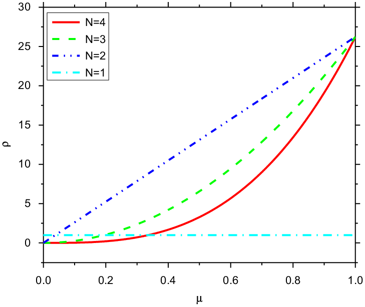
Equations (13) and (14) show that the look angle and its rate are functions of the dimensionless relative distance
 $\,\mu $
, which would decrease from one to almost zero for a successful attack when
 $\,r \lt \varepsilon $
,
 $\varepsilon $
is a minimal positive real number. The value of proportional coefficient
 $N$
plays an important role. This value is the border between positive and negative look angle rates when
 ${N_p} = 1$
. When the navigation gain
 ${N_p} \lt 1$
, the missile velocity vector will be far from the LOS; when the navigation gain
 $N \gt 1$
, the velocity vector will coincide with the LOS. Look angle curves for various navigation gains are plotted in Fig. 3.
Look angle variations.

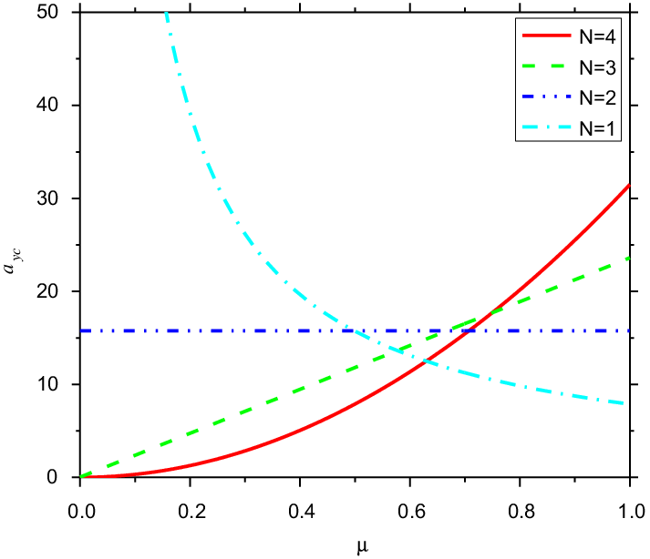
Substituting Equations (8) and (10) into Equation (14), the flight path angular rate, which is a scaled form of the acceleration command, is
 \begin{align}\dot \theta = - \frac{{{N_p}{V_M}\sin {\rho _{p,0}}}}{{{r_0}}}{\mu ^{N - 2}}.\end{align}
This equation indicates that the limiting value of the navigation gain is 2. Low gains (
 ${N_p} \lt 2$
) will result in unbounded acceleration profiles, which will inevitably lead to non-zero miss distance. With high gains (
 ${N_p} \gt 2$
), the final acceleration can converge to zero. This valuable conclusion implies that the condition
 ${N_p} \gt 2$
should be satisfied in later analysis to ensure that the final accelerations converge to zero and the guidance law is stable. This conclusion does not mean that the gain should always satisfy
 ${N_p} \gt 2$
in the entire process of flight. For the gain coefficient variable proportional guidance law to achieve different impact angles, the PN coefficient may be less than 1 at the beginning stage. For example, in literature [Reference Tekin and Erer16] and [Reference Zhang, Tang and Guo20], the PN coefficient is less than 1 in the first stage. In literature [Reference Liu, Shen and Lu21], an optimised time-varying PN coefficient is obtained through convex optimisation, in which the navigation gain is negative in the preceding stage and gradually converges to a value
 ${N_p} \ge 2$
. The acceleration does not diverge, and the missile accurately hits the target, which shows that the guidance law is convergent. This shows that only if
 ${N_p} \gt 2$
is satisfied at the end of the guidance process, the guidance law can be converged. Acceleration command with dimensionless variable
 $\mu $
for various navigation gains is plotted in Fig. 4.
Acceleration command variations.

3.0 Time-varying navigation gain guidance law for impact angle constraint
In this section, the impact angle constraint in longitudinal plane is deduced with time-varying navigation gain firstly. Then, the analysis is extended to a 3D plane to try to satisfy lateral angle constraint. However, the integral operator in lateral plane couples longitudinal information, which brings difficulty to lateral impact angle constraint when longitudinal motion is dominant. For practical application, the longitudinal motion is dominant; therefore, the guidance command in longitudinal plane guarantees precise hitting in a specific impact angle and that in lateral plane ensures accurate hitting.
3.1 Longitudinal plane guidance law
First, a time-varying navigation gain for specific impact angle constraints in longitudinal plane is considered. Define
 \begin{align}\,{\eta _p} = \sin {\rho _p},\,\, - 90^\circ \le {\rho _p} \le 90^\circ{,} \end{align}
where
 $\,{\eta _p}$
is the sine function of look angle in longitudinal plane and corresponds to a unique
 $\,{\rho _p}$
. Therefore,
 $\,{\eta _p}$
can represent the magnitude of the look angle in longitudinal plane. Assume the navigation gain
 ${N_p}$
(in longitudinal plane) is a function of
 ${\eta _p}$
as
 ${N_p} = {N_p}({\eta _p})$
.
Equation (10) is integrated on both sides from initial to final time
 \begin{align}\int_{{\eta _{p,0}}}^{{\eta _{p,f}}} {d{q_p}} = \int_{{\eta _{p,0}}}^{{\eta _{p,f}}} {\frac{1}{{{N_p}({\eta _p}) - 1}}} d{\rho _p}.\end{align}
In Equation (17),
 ${\eta _{p,0}}$
is the initial value of
 $\,{\eta _p}$
, while
 ${\eta _{p,f}}$
is the terminal value. Then,
 \begin{align}\left. {{q_p}} \right|_{{\eta _{p,0}}}^{{\eta _{p,f}}} = \int_{{\eta _{p,0}}}^{{\eta _{p,f}}} {\frac{1}{{{N_p}({\eta _p}) - 1}}} d{\rho _p}.\end{align}
Given that
 $\,{\eta _p} = \sin {\rho _p}$
,
 \begin{align}\,d{\rho _p} = \frac{1}{{\sqrt {1 - \eta _p^2} }}d{\eta _p}.\end{align}
Equation (19) is substituted into Equation (18), which yields
 \begin{align}\left. {{q_p}} \right|_{{\eta _{p,0}}}^{{\eta _{p,f}}} = \int_{{\eta _{p,0}}}^{{\eta _{p,f}}} {\frac{1}{{{N_p}({\eta _p}) - 1}}} \frac{1}{{\sqrt {1 - \eta _p^2} }}d{\eta _p}.\end{align}
 $r \to 0$
exists at impact moment to collision with the target. For the stationary target, the velocity direction coincides with the line of sight [Reference Ratnoo and Ghose10]. Therefore,
 $\,{\eta _{p,f}} \to 0$
exists, and the following can be obtained:
 \begin{align}{\theta _f} = {q_{p,f}} = {q_{p,0}} + \int_{{\eta _{p,0}}}^{{\eta _{p,f}}} {\frac{1}{{{N_p}({\eta _p}) - 1}}} \frac{1}{{\sqrt {1 - \eta _p^2} }}d{\eta _p},\end{align}
where
 ${q_{p,f}}$
denotes the terminal LOS angle, and
 ${q_{p,0}}$
is the initial LOS angle in longitudinal plane. From the conclusion in Section 2,
 ${\eta _p}$
will reduce monotonicity if
 $\,{N_p}({\eta _p}) \gt 1$
, and if
 $\,{N_p}({\eta _p}) \gt 2$
is satisfied, the final acceleration can be converged to zero. Therefore, the convergence PN gain should be larger than 2, which provides the principles of design parameters in the latter paper.
From Equation (21), the desired impact angle by a time-varying gain can be obtained through the design of the integral term. First, considering a specific linear function, the form of the function is heuristically proposed.
Assume
 \begin{align}\,\frac{1}{{{N_p}({\eta _p}) - 1}}\frac{1}{{\sqrt {1 - \eta _p^2} }} = a{\eta _p} + b.\end{align}
In Equation (22),
 $a$
and
 $b$
are the design parameters. Through this equation,
 ${N_p}({\eta _p})$
is known to be a function of
 ${\eta _p}$
, where
 \begin{align}{N_p}({\eta _p}) = 1/((a{\eta _p} + b)\sqrt {1 - \eta _p^2} ) + 1.\end{align}
From Equation (23), the PN gain, which is evidently time-varying, is determined via acquired look angle messages in flight process. For stationary target, when the missile hits the target,
 $\,{\eta _{p,f}} \to 0$
exists.
From Equation (23),
 \begin{align}\,{N_p}({\eta _p}) \to \frac{1}{b} + 1,{\rm{when}}\,\,\,\,{\eta _{p,f}} \to 0.\end{align}
Therefore, the parameter
 $b$
decides the navigation gain when the missile hits the target.
 ${N_p}({\eta _p}) \gt 2$
should be satisfied when the missile hits the target to make the final acceleration converge to zero. This condition restricts the choice of parameter
 $b$
.
Remark 1. From Equation (24), when
 $b = 0.5$
,
 ${N_p}({\eta _p}) \to 3$
exists when the missile hits the target, which implies that the final acceleration of the missile will converge to zero; when
 $b = 1$
,
 ${N_p}({\eta _p}) \to 2$
exists when the missile hits the target, which implies that the final acceleration maintains a fixed value. When
 $b = 2$
,
 ${N_p}({\eta _p}) \to 1.5$
exists when the missile hits the target, which implies that the final acceleration of the missile will diverge. Therefore,
 $b = 0.5$
is first chosen as a design parameter; thus, the terminal navigation gain
 ${N_p}$
guarantees the convergence of acceleration. Meanwhile, any
 $b$
can also be chosen for any intended convergence
 ${N_p}({\eta _p})$
.
Through the integral term in Equation (21),
 \begin{align}\int_{{\eta _{p,0}}}^{{\eta _{p,f}}} {\frac{1}{{{N_p}({\eta _p}) - 1}}} \frac{1}{{\sqrt {1 - \eta _p^2} }}d{\eta _p} = \int_{{\eta _{p,0}}}^{{\eta _{p,f}}} {(a{\eta _p} + b} )d{\eta _p} = - \left(a\eta _0^2 + b{\eta _0}\right).\end{align}
Then, the desired impact angle is
 \begin{align}{\theta _f} = {q_{p,f}} = {q_{p,0}} - \left( {a\eta _0^2 + b{\eta _0}} \right).\end{align}
Through the selected parameter
 $b$
, the expression of parameter
 $a$
is obtained as follows:
 $$a = {{({q_{p,f}} - {q_{p,0}}) + {\raise0.7ex\hbox{$1$} \!\mathord{\left/ {\vphantom {1 2}}\right.\,\,}\!\lower0.7ex\hbox{$2$}}{\eta _{p,0}}} \over { - {\raise0.7ex\hbox{$1$} \!\mathord{\left/ {\vphantom {1 2}}\right.\,\,}\!\lower0.7ex\hbox{$2$}}\eta _{p,0}^2}}.$$
Equation (27) shows that parameter
 $a$
depends on the initial flight parameters
 ${q_{p,0}}$
,
 ${\eta _{p,0}}$
, and terminal constraints
 ${q_{p,f}}$
.
The time-varying navigation gain can be obtained by substituting Equation (23) into Equation (27); thus, the expected impact angle can be obtained through the navigation gain.
Remark 2.
 $\,\frac{1}{{{N_p}({\eta _p}) - 1}}\frac{1}{{\sqrt {1 - \eta _p^2} }} = a\eta _p^2 + b{\eta _p} + c$
can also be selected, where
 $b$
and
 $c$
are design parameters and
 $a$
is calculated via integral term in Equation (25). In this scene, parameter
 $c$
determines the convergence navigation gain. If parameters
 $b = 0.5$
and
 $c = 0.5$
are selected, then
 $$a = {{({q_{p,f}} - {q_{p,0}}) + {\raise0.7ex\hbox{$1$} \!\mathord{\left/
{\vphantom {1 4}}\right.\,\,}
\!\lower0.7ex\hbox{$4$}}\eta _{p,0}^2 + {\raise0.7ex\hbox{$1$} \!\mathord{\left/
{\vphantom {1 2}}\right.\,\,}
\!\lower0.7ex\hbox{$2$}}{\eta _{p,0}}} \over { - {\raise0.7ex\hbox{$1$} \!\mathord{\left/
{\vphantom {1 3}}\right.\,\,}
\!\lower0.7ex\hbox{$3$}}\eta _{p,0}^3}}.$$
Remark 3. Suppose
 $\,{N_T},{N_M}$
are the constants, let
 \begin{align}N(\eta ) = \left\{ \begin{array}{l}{N_M}\quad{\eta _p}\;{\rm{ from }}\;{\eta _{p,0}}\;{\rm{ to }}\;{\eta _{p,s}}{\rm{ }}\\[5pt]{N_T}\quad{\eta _p}\;{\rm{ from }}\;{\eta _{p,s}}\;{\rm{ to }}\;{\eta _{p,f}}{\rm{ }}\end{array} \right.{,}\end{align}
where
 ${\eta _{p,0}}$
,
 ${\eta _{p,s}}$
, and
 ${\eta _{p,f}}$
represent the initial, middle, and final points of the flight process, respectively.
 \begin{align}{q_{p,f}} - {q_{p,0}} &= \left. q \right|_{{\eta _{p,0}}}^{{\eta _{p,f}}} = \left. q \right|_{{\eta _{p,0}}}^{{\eta _{p,s}}} + \left. q \right|_{{\eta _{p,s}}}^{{\eta _{p,f}}} = \int_{{\eta _{p,0}}}^{{\eta _{p,s}}} {\dfrac{1}{{{N_p}({\eta _p}) - 1}}} \dfrac{1}{{\sqrt {1 - \eta _p^2} }}d{\eta _p} + \int_{{\eta _{p,s}}}^{{\eta _{p,f}}} {\dfrac{1}{{{N_p}({\eta _p}) - 1}}} \dfrac{1}{{\sqrt {1 - \eta _p^2} }}d{\eta _p}\nonumber \\[5pt]&=\left. {\dfrac{1}{{{N_p}({\eta _p}) - 1}}\arcsin {\eta _p}} \right|_{{\eta _{p,0}}}^{{\eta _{p,s}}} + \left. {\dfrac{1}{{{N_p}({\eta _p}) - 1}}\arcsin {\eta _p}} \right|_{{\eta _{p,0}}}^{{\eta _{p,f}}}\nonumber\\[5pt]&=\dfrac{{{\rho _{p,s}}}}{{{N_M} - 1}} - \dfrac{{{\rho _{p,0}}}}{{{N_M} - 1}} + \dfrac{{{\rho _{p,f}}}}{{{N_T} - 1}} - \dfrac{{{\rho _{p,s}}}}{{{N_T} - 1}}.\end{align}
At the final point,
 ${\rho _{p,f}} = 0$
; therefore,
 \begin{align}{q_{p,f}} - {q_{p,0}} = \frac{{{\rho _{p,s}}}}{{{N_M} - 1}} - \frac{{{\rho _{p,0}}}}{{{N_M} - 1}} + 0 - \frac{{{\rho _{p,s}}}}{{{N_T} - 1}}.\end{align}
The following can be obtained:
 \begin{align}{q_{p,f}} = {q_{p,0}} - \frac{{{\rho _{p,0}}}}{{{N_M} - 1}} + {\rho _{p,s}}\frac{{{N_T} - {N_M}}}{{({N_M} - 1)({N_T} - 1)}}.\end{align}
Therefore, the two-phase PPN in literature [Reference Tekin and Erer16] is a special case for the time-varying navigation gain guidance law.
3.2 Lateral plane guidance law
Similar to longitudinal plane, the missile is guided by PPN in lateral plane, and the guidance equation is
 \begin{align}{a_{zc}} = {N_y}{V_M}{\dot q_y},\end{align}
where
 ${N_y}$
and
 ${\dot q_y}$
are the PN coefficient and the LOS angular velocity in lateral plane, respectively. For the change rate of flight deflection angle,
 \begin{align}{\dot \psi _v} = \frac{{{a_{zc}}}}{{ - {V_M}\cos \theta }}.\end{align}
Equation (34) can be rewritten as:
 \begin{align}{\dot \psi _v} = \frac{{{N_y}\,{{\dot q}_y}}}{{ - \cos \theta }}.\end{align}
Differentiating Equation (4):
 \begin{align}{\dot \rho _y} = {\dot \psi _v} - {\dot q_y}.\end{align}
Combining Equations (35) and (36) leads to the following:
 \begin{align}{\dot \rho _y} = \left( {\frac{{{N_y}}}{{ - \cos \theta }} - 1} \right){\dot q_y}.\end{align}
Let
 \begin{align}{\eta _y} = \sin {\rho _y},\, - 90^\circ \le {\rho _y} \le 90^\circ{,}\end{align}
where
 $\,{\eta _y}$
is the sine function of look angle in lateral plane, which also corresponds to a unique
 $\,{\rho _y}$
and can represent the magnitude of the look angle in lateral plane. Navigation gain
 ${N_y}$
in lateral plane is assumed as a function of
 ${\eta _y}$
as
 $\,{N_y} = {N_y}({\eta _y})$
.
Equation (37) is integrated on both sides from initial to final time
 \begin{align}\int_{{\eta _{y,0}}}^{{\eta _{y,f}}} {d{q_y}} = \int_{{\eta _{y,0}}}^{{\eta _{y,p}}} {\frac{1}{{\dfrac{{{N_y}({\eta _y})}}{{ - \cos \theta }} - 1}}} d{\rho _y}.\end{align}
In Equation (39),
 ${\eta _{y,0}}$
is the initial value of
 $\,{\eta _y}$
while
 ${\eta _{y,f}}$
is the terminal value. Then,
 \begin{align}\left. {{q_y}} \right|_{{\eta _{y,0}}}^{{\eta _{y,f}}} = \int_{{\eta _{y,0}}}^{{\eta _{y,f}}} {\frac{1}{{\dfrac{{{N_y}({\eta _y})}}{{ - \cos \theta }} - 1}}} d{\rho _y}.\end{align}
Given that
 $\,{\eta _y} = \sin {\rho _y}$
,
 \begin{align}\,d{\rho _y} = \frac{1}{{\sqrt {1 - \eta _y^2} }}d{\eta _y}.\end{align}
Equation (41) is substituted into Equation (40), which yields
 \begin{align}\left. {{q_y}} \right|_{{\eta _{y,0}}}^{{\eta _{y,f}}} = \int_{{\eta _{y,0}}}^{{\eta _{y,f}}} {\frac{1}{{\dfrac{{{N_y}({\eta _y})}}{{ - \cos \theta }} - 1}}} \frac{1}{{\sqrt {1 - \eta _y^2} }}d{\eta _y}.\end{align}
Equation (42) shows that the integral operator contains the
 $\cos \theta $
, which is the guidance information in longitudinal plane.
 $\cos \theta $
changes with the dynamic in the flight process, and no analytical relation between
 $\cos \theta $
and
 ${\eta _y}$
exists, therefore, calculating the integral term is difficult. Achieving the impact angle constraints in lateral plane is also complicated when the longitudinal motion is dominant. For a realistic three-dimensional guidance scenario, the guidance command in longitudinal motion is dominant, so the impact angle constraints are mainly conducted in longitudinal plane and for lateral plane, a proportional guidance law shown in Equation (33) can be adopted to achieve precise attack.
Remark 4. If the effect of
 $\cos \theta $
in lateral plane is ignored, that is to say,
 ${\dot \psi _v} = \frac{{{a_{zc}}}}{{{V_M}}}$
, which demonstrates that the lateral and longitudinal planes are completely symmetrical, then
 \begin{align}\left. {{q_y}} \right|_{{\eta _{y,0}}}^{{\eta _{y,f}}} = \int_{{\eta _{y,0}}}^{{\eta _{y,f}}} {\frac{1}{{{N_y}({\eta _y}) - 1}}} \frac{1}{{\sqrt {1 - \eta _y^2} }}d{\eta _y}.\end{align}
By using the same method as the longitudinal plane, the time-varying navigation gain in lateral plane is obtained as shown in Equation (44).
 \begin{align}{N_y}({\eta _y}) = 1/((a{\eta _y} + b)\sqrt {1 - \eta _y^2} ) + 1.\end{align}
In Equation (44), where
 $b = 0.5$
,
 $a = \left( {({q_{y,f}} - {q_{y,0}}) + {\raise0.7ex\hbox{$1$} \!\mathord{\left/ {\vphantom {1 2}}\right.\,\,}\!\lower0.7ex\hbox{$2$}}{\eta _{y,0}}} \right)/ - {\raise0.7ex\hbox{$1$} \!\mathord{\left/ {\vphantom {1 2}}\right.\,\,}\!\lower0.7ex\hbox{$2$}}\eta _{y,0}^2$
,
 ${q_{y,f}}$
is the expected LOS angle (impact angle),
 ${q_{y,0}}$
is the initial LOS angle, and
 ${\eta _{y,0}}$
is the initial look angle, which are all in the lateral plane. In a 3D plane simulation, the results show that when the
 $\theta $
in the longitudinal plane is relatively large (or when longitudinal motion is dominant), a deviation always exists between the actual and expected impact angles in lateral plane. When the
 $\theta $
in the longitudinal plane is relatively small (or the missile moves on the horizontal level), the lateral impact angle constraints can be well satisfied. It is needed to point out when longitudinal and lateral impact angle are restrained simultaneously, the lateral angle constraints don’t affect the accuracy of longitudinal angle constraints.
4.0 Numerical simulations
Several nonlinear simulations are conducted in an air-to-surface terminal guidance scenario in longitudinal and lateral planes to investigate the characteristics of the proposed guidance law. Cases 1 to 4 are emulated in longitudinal plane to reveal the efficiency of the proposed guidance law. Case 5 is extended to 3D plane to further illustrate the effectiveness of the proposed method with the presence of measurement noises and model deviation simultaneously, and to verify whether the effect of lateral motion affects the longitudinal guidance accuracy. The simulation results and analyses are exhibited afterward. In the given attack conditions in longitudinal plane, a missile has an initial speed of 300m/s, with the initial position
 $\,{x_{M0}}$
= 0m,
 ${y_{M0}}$
= 10,000m and initial flight path angle
 $\,{\theta _{M0}} = 20^\circ $
to strike a stationary target. The initial position of the target is
 ${x_{T0}}$
= 17,320m,
 ${y_{T0}}$
= 0m. The initial LOS angle is
 $\,{q_{M0}} = - 30^\circ $
; therefore, the initial look angle is
 $\,{\rho _{M0}} = 50^\circ $
. The normal acceleration limitation is
 $\,\left| {a_{yc}^{\max }} \right| = 2g$
(approximately 19.6
 $\textrm{m}/{\textrm{s}^2}$
). The simulation step size is 10 ms, the parameter
 $b = 0.5$
, and the parameter
 $a$
is calculated through Equation (27). For a given desired impact angle (or LOS angle), a time-varying navigation gain is applied.
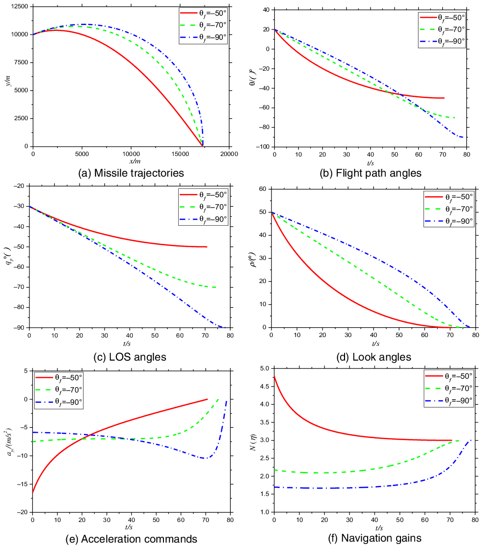
Case 1 (ideal models for various desired LOS angles). Simulations for various terminal LOS angles with constant velocity and no autopilot lag are performed in this case. Figure 5 depicts the performance of the proposed guidance law with various desired LOS angles. Figure 5(a) exhibits the trajectories resulting from the proposed guidance strategy. The trajectories satisfy the different LOS angle constraints and engage the stationary target. The LOS angles (or flight path angles) also strictly satisfy the constraints, which can be clearly observed in Fig. 5(b) and (c). Figure 5(d) shows that the look angles converge to zero for stationary target under the proposed guidance law, which illustrates that the final missile heads toward the target. Figure 5(e) reveals that the acceleration commands for various terminal LOS angles converge to zero continuously and smoothly. Figure 5(f) shows that the navigation gains are always larger than 1 and finally converge to 3, resulting in a monotonously decrease of look angles.
Simulation results for Case 1.

Case 2 (comparative cases with other guidance laws). The performance of the proposed guidance scheme is compared with the BPN guidance law in Ref. [Reference Kim, Lee and Han9] and a switched-gain guidance law (SGGL) described in Ref. [Reference Tekin and Erer16], which is illustrated in Fig. 5 with the desired LOS angle constraints of
 ${q_f} = - 90^\circ $
. The implemented acceleration command in Refs (Reference Kim, Lee and Han9,Reference Tekin and Erer16) are summarised as
 \begin{align}{a_{yc}} = {N_1}{V_M}{\dot q_p} + {N_2}{V_M}({{q_p} - {q_d}})/({{t_f} - t}),\end{align}
where
 ${q_d}$
is the desired LOS angle.
 ${N_1}$
and
 ${N_2}$
are navigation coefficients.
 ${N_1}\,=\,4$
and
 ${N_2}\,=\,2$
.
 \begin{align}{a_{yc}} = \left\{ \begin{array}{l}{N_M}{V_M}{{\dot q}_p}\,\,\,\,\,\,\,\,\,\,\,\,\,\,\,\,{\rm{if}}\,\,\,\,\,\,\Gamma \gt {q_d}\\[5pt]{N_T}{V_M}{{\dot q}_p}\,\,\,\,\,\,\,\,\,\,\,\,\,\,\,\,\,\,{\rm{if}}\,\,\,\,\,\,\Gamma \le {q_d}\end{array} \right.{,}\end{align}
where
 $\Gamma = {q_p} - \frac{{{\rho _p}}}{{{N_T} - 1}}$
, and
 ${N_M}$
and
 ${N_T}$
are navigation coefficients.
 ${N_M}\,=\,0.583$
and
 ${N_T}\,=\,2$
.
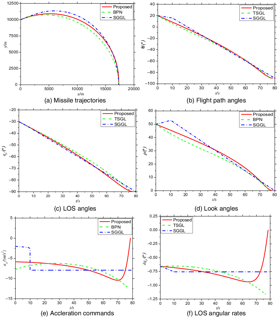
In Fig. 6(a), it is obvious the trajectories of three guidance law hit the target accurately. For the terminal angle constraint, all the methods can satisfy the demand as shown in Fig. 6(b) and (c). The look angle variations are quite distinct from each other as observed in Fig. 6(d). The SGGL, as a special situation of the proposed guidance law, has an increase in look angle in initial phase to hit the target. Therefore, if the seeker’s field of view (FOV) limitation is considered, then the increase of the SGGL is not beneficial. In Fig. 6(e), compared with the SGGL, the acceleration produced by the proposed method appears smoothly and converge to zero, which is conducive to the final attack. However, the SGGL has a sudden change in the switching point, and the terminal phase of BPN has considerable acceleration. Both are unfavorable for guidance systems. The conclusion is proven again in Fig. 6(f).
Simulation results for Case 2.

Case 3 (comparative cases considering first-order lag of autopilot). Several simulation cases for the guidance law in Refs (Reference Kim, Lee and Han9,Reference Tekin and Erer16) and the proposed one in this study are conducted to compare the performance with respect to autopilot lag. A first-order lag system, which can be described with a time constant
 ${T_\alpha }$
, is considered in this case.
 \begin{align}\frac{{{a_y}}}{{{a_{yc}}}} = \frac{1}{{{T_\alpha }s + 1}},\end{align}
where
 ${a_y}$
and
 ${a_{yc}}$
represent the lagged system response and the acceleration command, respectively.
 ${T_\alpha }$
is set to vary from 0 to 0.5 with the terminal LOS angle of −90°. Comparative results of
 ${T_\alpha } = 0.5$
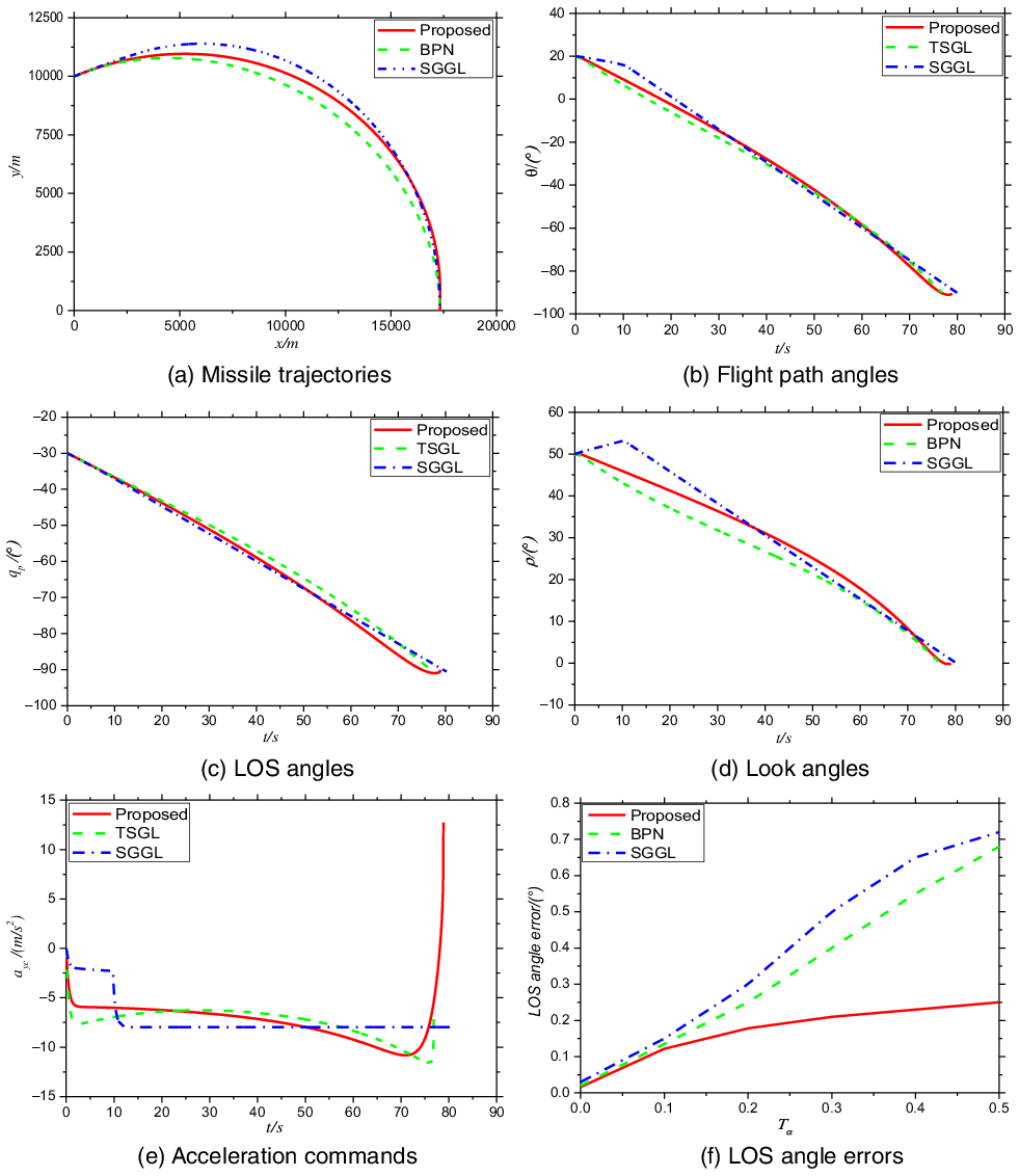
are illustrated in Fig. 7. When the autopilot lag is considered, Fig. 7(a), (b), (c), and (d) show that the missile simultaneously satisfies the hit point and LOS angle constraints through three guidance laws. The proposed method notably has a positive trend in acceleration command at the end of the engagement because the LOS angle exceeds −90°; therefore, the command pulls the angle back. The LOS angle error (LAE) is described in Fig. 7(f) with the variation of
 ${T_\alpha }$
. The LAE of the proposed guidance law in this work is less than that of Refs (Reference Kim, Lee and Han9,Reference Tekin and Erer16) for each investigated value of
 ${T_\alpha }$
. The different trends of the three curves shown in Fig. 7 indicate that compared with Refs (Reference Kim, Lee and Han9,Reference Tekin and Erer16), the influence on the proposed method unnoticeably varies with the increasing of
 ${T_\alpha }$
. The LAE of the proposed guidance law can maintain a small value.
Simulation results for Case 3.

Case 4 (realistic missile model cases). In this case, additional simulations are conducted with a realistic missile model. The aerodynamics drag and gravity are considered in the realistic missile model, which is taken from Ref. [Reference Kee, Li and Chai22]. The nonlinear dynamics equations are given by
 \begin{align}\begin{array}{l}{{\dot x}_M} = {V_M}\cos {\theta _M}\\[5pt]{{\dot y}_M} = {V_M}\sin {\theta _M}\\[5pt]{{\dot V}_M} = \dfrac{{{T_M} - {D_M}}}{m} - g\sin {\theta _M}\\[5pt]{{\dot \theta }_M} = \dfrac{{{a_{yc}} - g\cos {\theta _M}}}{{{V_M}}}\end{array}.\end{align}
In Equation (48), the missile mass is
 $m = 100$
kg. Without loss of generality, the thrust
 ${T_M} = 0$
in the terminal guidance process (at the beginning of the simulation) is assumed. The air drag force
 ${D_M} = \frac{1}{2}{c_d}\rho V_M^2S$
,
 $S = 1$
is the reference area,
 $\rho $
is the air density, and
 ${c_d}$
is the air drag coefficient. Furthermore, the gravity compensation term should be added to the original acceleration command to set-off the gravity influence on the flight path angle. For realistic implementation, the original acceleration command must be changed as follows:
 \begin{align}{a_{yc}} = a_{yc}^ * + g\cos {\theta _M},\end{align}
where
 $a_{yc}^ * $
represents the acceleration command for the models without gravity compensation. Different terminal angle constraints are simulated under the aforementioned realistic model. The detailed simulation results are displayed in Fig. 8.
Simulation results for Case 4.

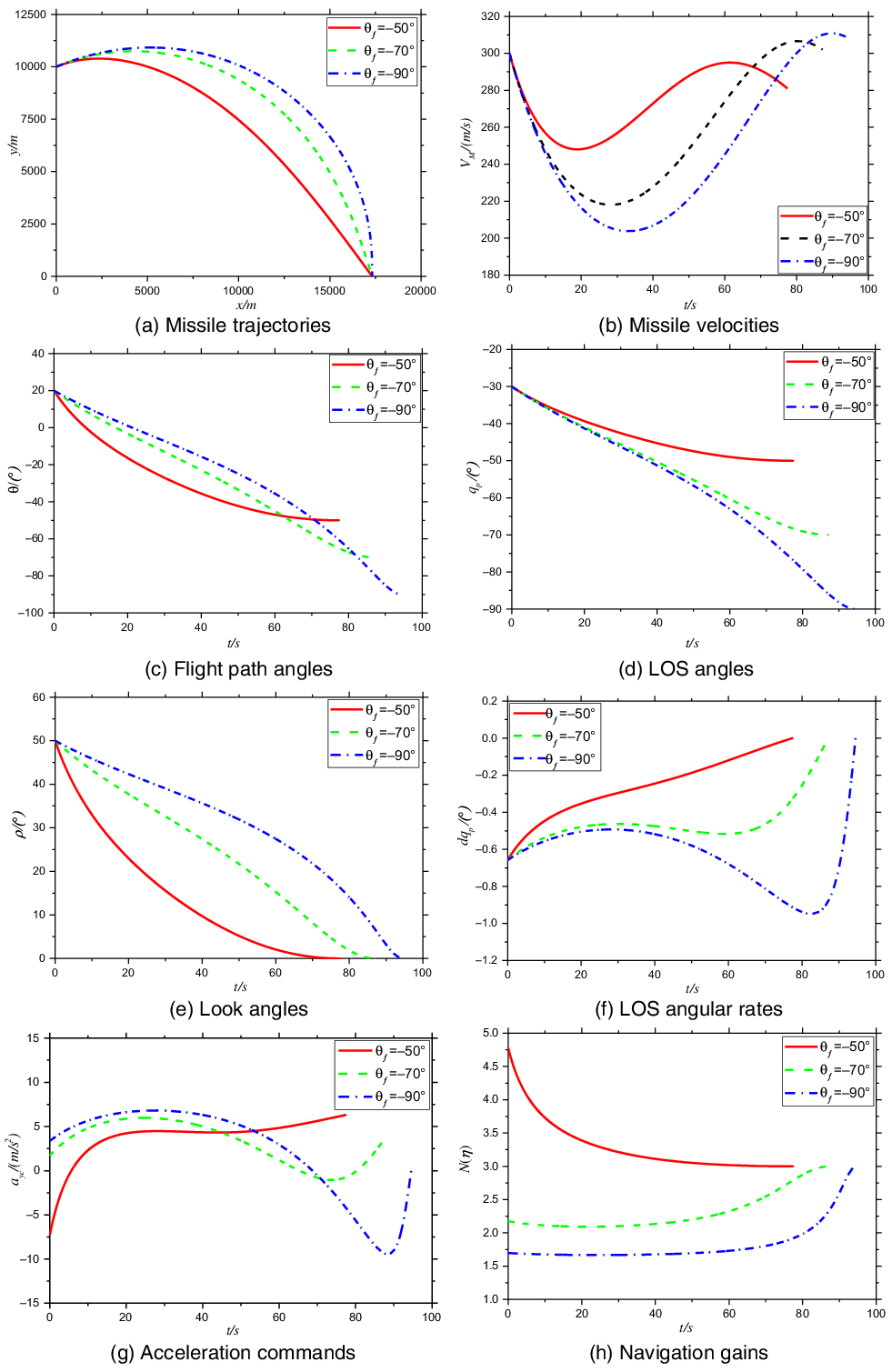
Figure 8(a) shows that the missile can successfully hit the target with realistic missile model. In Fig. 8(b), the missile velocities vary due to the gravity and air drag, and the velocities increase during the flight because of the initial potential energy. The main influences on flight path, LOS, and look angles are exhibited in Fig. 8(c), 8(d), and 8(e), respectively. The terminal constraints are strictly satisfied. From Fig. 8(f), the LOS angular rates converge near zero. The acceleration histories are plotted in Fig. 8(g). High impact angle constraint clearly needs large maximum acceleration effect on the missile at the end of the flight, especially for the realistic missile model. From Fig. 8(h), the navigation gains are also larger than 1 and ultimately converge to 3, which results in the monotonically decreasing of look angles.
Simulation results for Case 5.

Case 5 (realistic missile model in 3D plane considering measurement noises and model deviations). In this case, the initial conditions of the missile to strike a stationary target in 3D plane are described as follows. The initial speed of the missile is also 300m/s with the initial position
 ${x_{M0}}$
= 0m,
 ${y_{M0}}$
= 10,000m,
 ${z_{M0}}$
= 0m, and initial flight path angle
 $\,{\theta _{M0}} = 20^\circ $
, flight deflection angle
 ${\psi _{v,M0}} = 10^\circ $
. The initial position of the target is
 ${x_{T0}}$
= 17,320m,
 ${y_{T0}}$
= 0m.
 ${z_{T0}}$
= 1,000m. The normal acceleration limitations are
 $\,\left| {a_{yc}^{\max }} \right| = 2g$
(approximately 19.6
 $\textrm{m}/{\textrm{s}^2}$
) and
 $\,\left| {a_{zc}^{\max }} \right| = 2g$
(approximately 19.6
 $\textrm{m}/{\textrm{s}^2}$
). The realistic dynamic model of the missile is similar to that of Case 4. The nonlinear dynamics equations in 3D plane are given by
 \begin{align}\begin{array}{l}{{\dot x}_M} = {V_M}\cos {\theta _M}\cos {\psi _v}\\[5pt]{{\dot y}_M} = {V_M}\sin {\theta _M}\\[5pt]{{\dot z}_M} = - {V_M}\cos {\theta _M}\sin {\psi _v}\\[5pt]{{\dot V}_M} = \dfrac{{ - {D_M}}}{m} - g\sin {\theta _M}\\[5pt]{{\dot \theta }_M} = \dfrac{{{a_{yc}} - g\cos {\theta _M}}}{{{V_M}}}\\[5pt]{{\dot \psi }_v} = \dfrac{{ - {a_{zc}}}}{{{V_M}\cos {\theta _M}}}\end{array}.\end{align}
Meanwhile, measurement noises and model deviation exist in the system. For the realistic model, the measurement errors may be introduced by the seeker, and the LOS angular rate extracted by the seeker may have noises. The noises from the seeker are
 $\delta {q_p}$
and
 $\delta {q_y}$
in longitudinal and lateral planes, respectively.
 $\delta {q_p}$
and
 $\delta {q_y}$
are random numbers subjected to normal distribution and denoted as
 $\delta {q_p}\sim N\left( {0,{\sigma _p}} \right)$
and
 $\delta {q_y}\sim N\left( {0,{\sigma _y}} \right)$
, respectively;
 ${\sigma _p}$
and
 ${\sigma _y}$
are standard deviations that satisfy
 $\,3{\sigma _p} = 2\% $
and
 $\,3{\sigma _y} = 1\% $
, respectively. During the flight process, the air drag force may exhibit model deviation
 $\delta {c_d}$
, which is denoted as
 $\delta {c_d}\sim N\left( {0,{\sigma _{{c_d}}}} \right)$
, and
 $\,3{\sigma _{{c_d}}} = 20\% $
. Therefore, realistic guidance information and model are denoted by Equation (51)
 \begin{align}\begin{array}{l}{{\dot q}_p} = \dot q_p^ * + \delta {{\dot q}_p}\\[5pt]{{\dot q}_y} = \dot q_y^ * + \delta {{\dot q}_y}\\[5pt]{c_d} = c_d^ * \left( {1 + \delta {c_d}} \right)\end{array},\end{align}
where
 $\dot q_p^ * $
,
 $\dot q_y^ * $
, and
 $c_d^ * $
are ideal guidance information and model,
 $\dot q_p^{}$
,
 $\dot q_y^{}$
, and
 $c_d^{}$
are realistic guidance information and model. The acceleration command in longitudinal and lateral planes denoted by Equation (52) must be changed as
 \begin{align}\begin{array}{l}{a_{yc}} = {N_p}{V_M}{{\dot q}_p} + g\cos {\theta _M}\\[5pt]{a_{zc}} = {N_y}{V_M}{{\dot q}_y}\end{array},\end{align}
where
 ${N_p}$
is the proposed time-varying navigation coefficient to accomplish specified impact angle, and
 ${N_y} = 3$
is used to achieve precise attack for the target. The simulation results are displayed in Fig. 9.
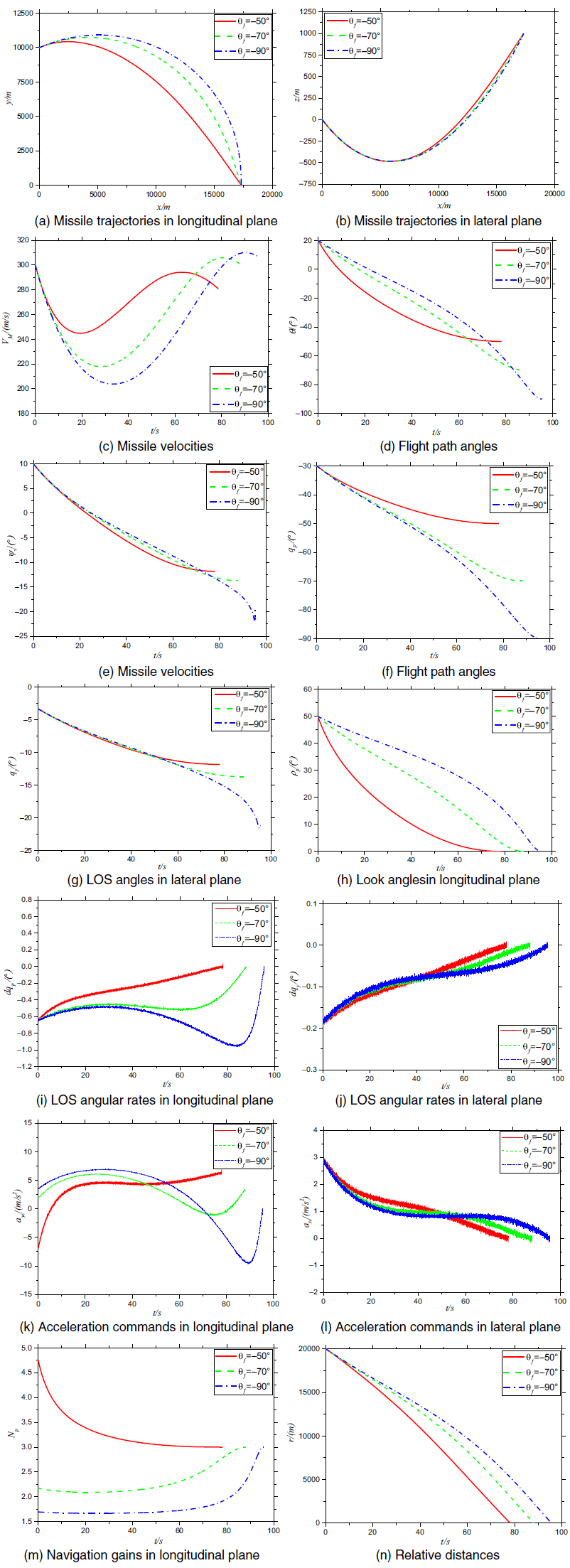
Figure 9(a), (b), and (n) show that the missile can successfully hit the target with realistic dynamic model considering seeker measurement noises and model deviation in a 3D plane. In Fig. 9(c), the missile velocities vary due to the gravity and air drag, and the velocities increase during the flight because of the initial potential energy. The main influences on flight path, LOS, and look angles are exhibited in Fig. 9(d) to (h). The terminal constraints are strictly satisfied even with the presence of various deviations, and the lateral motion would not influence guidance accuracy in longitudinal plane. From Fig. 9(i) and (j), measurement noises were observed in the LOS angular rates, and both converged near zero in longitudinal and lateral planes. The acceleration histories are plotted in Fig. 9(k) and (l). The measurement noises of the seeker are introduced into the guidance commands, which do not exceed the acceleration bounds. From Fig. 9(m), the navigation gains are also larger than 1 and ultimately converge to 3, which result in the monotonically decreasing of look angles and convergence of acceleration.
5.0 Conclusions
Aiming at the problems of achieving designated angle at the end of guidance process to improve attack power for the missiles, a new time-varying navigation gain guidance law is proposed in this paper for a stationary target in a 3D plane. The navigation gain is seen as a function of look angles, and the monotonicity of the look angle and the convergence of acceleration will influence the guidance strategy. Therefore, the monotonic and convergent characteristics are analysed as the bases of the proposed method. The proposed navigation gain has a continuous form, and estimating time-to-go, adding an additional bias term, or providing a switch strategy are unnecessary.
For the design of the guidance law, parameter
 $b$
has an influence on the convergent value of the navigation gain, thus affecting the convergence of acceleration. Therefore, choice of
 $b$
determines the convergence of the guidance command. The analysis is then extended to a 3D plane in an attempt to satisfy lateral angle constraint. However, the integral operator in lateral plane couples
 $\theta $
in longitudinal plane, which introduces difficulty in satisfying impact angle constraints in longitudinal and lateral planes simultaneously, especially when
 $\theta $
is relatively large. Finally, extensive simulations, including ideal models for various desired LOS angles, comparative cases with other guidance laws, comparative cases considering first-order lag of autopilot, realistic missile model cases, and realistic missile model in 3D plane considering measurement noises and model deviation, are performed. The results validate the efficiency of the proposed method. However, the time-varying navigation gain depends on sine function of look angle
 ${\eta _p}$
, so the direction information of velocity should be obtained, there may exist deviations in practical application. In addition, the interception of manoeuvering targets also needs to be considered in the future.