1 Introduction
Although the wing of an insect beats at high frequency (usually above 100 Hz), the velocity of the wing relative to the undisturbed air is small, owing to the small wing length. As a result, the vertical force coefficient of the wing required to balance the weight is relatively high; the mean vertical-force coefficient required is around 2 (Ellington Reference Ellington1984a ,Reference Ellington b ,Reference Ellington c ,Reference Ellington d ; Sun & Du Reference Sun and Du2003), about three times as large as that of a cruising airplane. This high vertical-force coefficient cannot be explained by conventional aerodynamics (which applies to the steady-state, high Reynolds number and attached flow).
Much work has been done to reveal the generation mechanisms of the high vertical-force coefficient (Sane Reference Sane2003; Wang Reference Wang2005; Shyy et al. Reference Shyy, Aono, Chimakurthi, Trizila, Kang, Cesink and Liu2010). It has been shown that insects use the lift of the wings to provide the weight-supporting vertical force (i.e. using lift principle for flight) and that the high lift is produced mainly by the leading-edge vortex (LEV) that attaches to the wing during an entire down- or upstroke, which is referred to as the delayed-stall mechanism (Ellington et al. Reference Ellington, van den Berg, Willmott, Ellington and Thomas1996; Liu et al. Reference Liu, Ellington, Kawachi, van den Berg and Willmott1998; Dickinson, Lehmann & Sane Reference Dickinson, Lehmann and Sane1999; Bomphrey et al. Reference Bomphrey, Srygley, Taylor and Thomas2002). The LEV, together with the root vortex, the trailing-edge vortex and the tip vortex, form a vortex loop. As the wing moves, the attached LEV facilitates a linear growth of the vortex loop with time, producing a large time rate of change of the first moment of vorticity (or fluid impulse), hence a large aerodynamic force (Sun & Wu Reference Sun and Wu2004). Because of the LEV’s essential role in the high-lift generation of a flapping wing at low Reynolds number, in recent years much work has been conducted to study its fluid-dynamic properties. These studies have revealed the detailed structure of the LEV and how it changes with the Reynolds number (e.g. Birch, Dickson & Dickson Reference Birch, Dickson and Dickson2004; Kim & Gharib Reference Kim and Gharib2010; Jardin, Farcy & David Reference Jardin, Farcy and David2012; Ozen & Rockwell Reference Ozen and Rockwell2012; Garmann, Visbal & Orkwis Reference Garmann, Visbal and Orkwis2013), the aspect ratio of the wing (e.g. Luo & Sun Reference Luo and Sun2005; Carr, Chen & Ringuette Reference Carr, Chen and Ringuette2013; Harbig, Sheridan & Thompson Reference Harbig, Sheridan and Thompson2013) and the wing shape (Wolfinger & Rockwell Reference Wolfinger and Rockwell2014), and have partially explained the stability of the LEV (here the word ‘stability’ is used to describe whether the LEV remains attached throughout the stroke (stable) or if it is shed (unstable); e.g. Lentink & Dickinson Reference Lentink and Dickinson2009, Shyy et al. Reference Shyy, Trizila, Kang and Aono2009, Wojcik & Buchholz Reference Wojcik and Buchholz2014).
However, the above results do not apply to the smallest insects because of the very large effect of air viscosity. The viscous effect on the flow around an insect wing depends on the Reynolds number (
 $Re$
), which is the ratio between inertial and viscous forces acting on a volume of air. The smaller the
 $Re$
, the larger the viscous effect.
 $Re$
is proportional both to the chord length and the relative velocity of the wing. As insect size becomes smaller, both these two values decrease.
 $Re$
therefore decreases with the decreasing insect-size. For the smallest insects such as the tiny wasp Encarsia formosa (the wing length is approximately 0.6 mm),
 $Re$
is approximately 10 (Weis-Fogh Reference Weis-Fogh1973). At this low
 $Re$
, the viscous effect is so large that the LEV is significantly defused and little lift can be generated, while the drag is large (Miller & Peskin Reference Miller and Peskin2004; Wu & Sun Reference Wu and Sun2004). Therefore, the smallest insects cannot use the same lift generation mechanisms as those of their larger counterparts, and they may not even use the lift principle for flight. That is, the smallest insects may use a drag mechanism for flight. That very small insects may use drag rather than lift for flight was suggested a long time ago by Horridge (Reference Horridge1956), but there were some arguments against it (Weis-Fogh Reference Weis-Fogh, Wu, Brokaw and Brennen1975). First, the drag principle was difficult to apply for the following reason: at very low
 $Re$
the drag of a wing tended to become independent of the angle of attack, hence the drag of the effective stroke might be cancelled by that of the return stroke, producing little net force. Second, people had never yet observed a small insect in flapping flight that used drag rather than lift. Weis-Fogh (Reference Weis-Fogh1973) found that the tiny wasp Encarsia formosa performed an unusual wing motion, ‘clap and fling’, and it was shown that the ‘fling’ can produce a momentary large vertical force (Spedding & Maxworthy Reference Spedding and Maxworthy1986). But because detailed quantitative data on wing kinematics were not readily available at the time, it was not known if the vertical force generated by the Weis-Fogh ‘fling’ was enough for weight support.
So far, how the smallest insects produce the weight-supporting vertical force, whether or not they use the drag principle for flight, and if the drag principle is used, how a net vertical force is generated at extremely low
 $Re$
, remain unknown.
In the present study, we first used high-speed cameras equipped with micro-lenses and extension tubes to measure the detailed wing kinematics in the tiny wasp Encarsia formosa, and then used a well-tested flow solver to solve the Navier–Stokes equations and obtained the flows and aerodynamic forces. We have achieved the following results: we find that in addition to the Weis-Fogh ‘fling’, there is another special wing kinematics, ‘rowing’: the wings stroke fast downward and backward at a large angle of attack, like the movement of the oars of a boat. It is shown that the rowing produces 70 % of the required vertical force, and the Weis-Fogh ‘fling’ produces the other 30 %. It is shown that the large vertical force by the rowing is generated by an unsteady-drag mechanism. We have observed for the first time tiny insects using drag to support their weight and we explain how a net vertical force is generated when the drag principle is applied.
2 Experimental and computational methods
2.1 Experimental systems and techniques
Encarsia formosa Gahan were acquired from the Laboratory of Biological Invasion of Institute of Plant Protection, Chinese Academy of Agricultural Sciences, which were descendants of wild-caught E. formosa. The wasps were housed in small chambers in groups of three to five individuals and fed with 20 % sugar solution. The flight of the wasps in a transparent flight chamber (
 $40\times 40\times 30~\text{mm}^{3}$
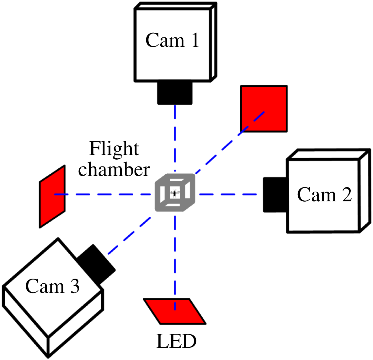
) was filmed using three orthogonally aligned synchronized high-speed cameras (FASTCAM Mini UX100, Photron Inc., San Diego, CA, USA; 10 000 frames per second, shutter speed
 $20~\unicode[STIX]{x03BC}\text{s}$
, resolution
 $896\times 488$
pixels) mounted on an optical table (figure 1). Each camera was equipped with a 60 mm micro-Nikkor lens and 12 mm extension tube. Each camera view was backlit using a 50 W integrated red light emitting diode (LED; luminous flux, 4000 lm; wavelength, 632 nm). The light was made uniform by two lenses. We manually triggered the synchronized cameras when the insect was observed to fly steadily in the filming area of approximately
 $4\times 4\times 4~\text{mm}^{3}$
, which represented the intersecting field of views of the three cameras. The experiment was conducted at room temperature
 $25{-}27\,^{\circ }\text{C}$
and relative humidity 50–60 %.
A sketch showing the experimental set-up: the flight chamber and cameras; each camera view is backlit using a integrated red light emitting diode (LED).

The method used to extract the three-dimensional (3-D) body and wing kinematics from the filmed data was a modification of that used in several previous works of our group (Liu & Sun Reference Liu and Sun2008; Mou, Liu & Sun Reference Mou, Liu and Sun2011). The original method and the modification are described in appendix A.
2.2 Methods of flow and aerodynamic-force computation
The flows around and the aerodynamic force acting on the insect were computed using the method of computational fluid dynamics. The governing equations of the flow are the incompressible Navier–Stokes equations, the dimensionless forms of which are
 $$\begin{eqnarray}\displaystyle & \unicode[STIX]{x1D735}\boldsymbol{\cdot }\boldsymbol{u}=0, & \displaystyle\end{eqnarray}$$
 $$\begin{eqnarray}\displaystyle & \displaystyle \frac{\unicode[STIX]{x2202}\boldsymbol{u}}{\unicode[STIX]{x2202}\unicode[STIX]{x1D70F}}+\boldsymbol{u}\boldsymbol{\cdot }\unicode[STIX]{x1D735}\boldsymbol{u}=-\unicode[STIX]{x1D735}p+\left(\frac{1}{Re}\right)\unicode[STIX]{x1D6FB}^{2}\boldsymbol{u}, & \displaystyle\end{eqnarray}$$
where
 $\boldsymbol{u}$
is the non-dimensional fluid velocity,
 $p$
the non-dimensional fluid pressure,
 $\unicode[STIX]{x1D70F}$
the non-dimensional time,
 $\unicode[STIX]{x1D735}$
the gradient operator,
 $\unicode[STIX]{x1D6FB}^{2}$
the Laplacian operator and
 $Re$
the Reynolds number; in the non-dimensionalization,
 $c$
,
 $U$
and
 $c/U$
are taken as reference length, velocity and time, respectively (here
 $c$
is the mean chord length of wing and
 $U$
is the mean flapping velocity at the radius of gyration of wing).
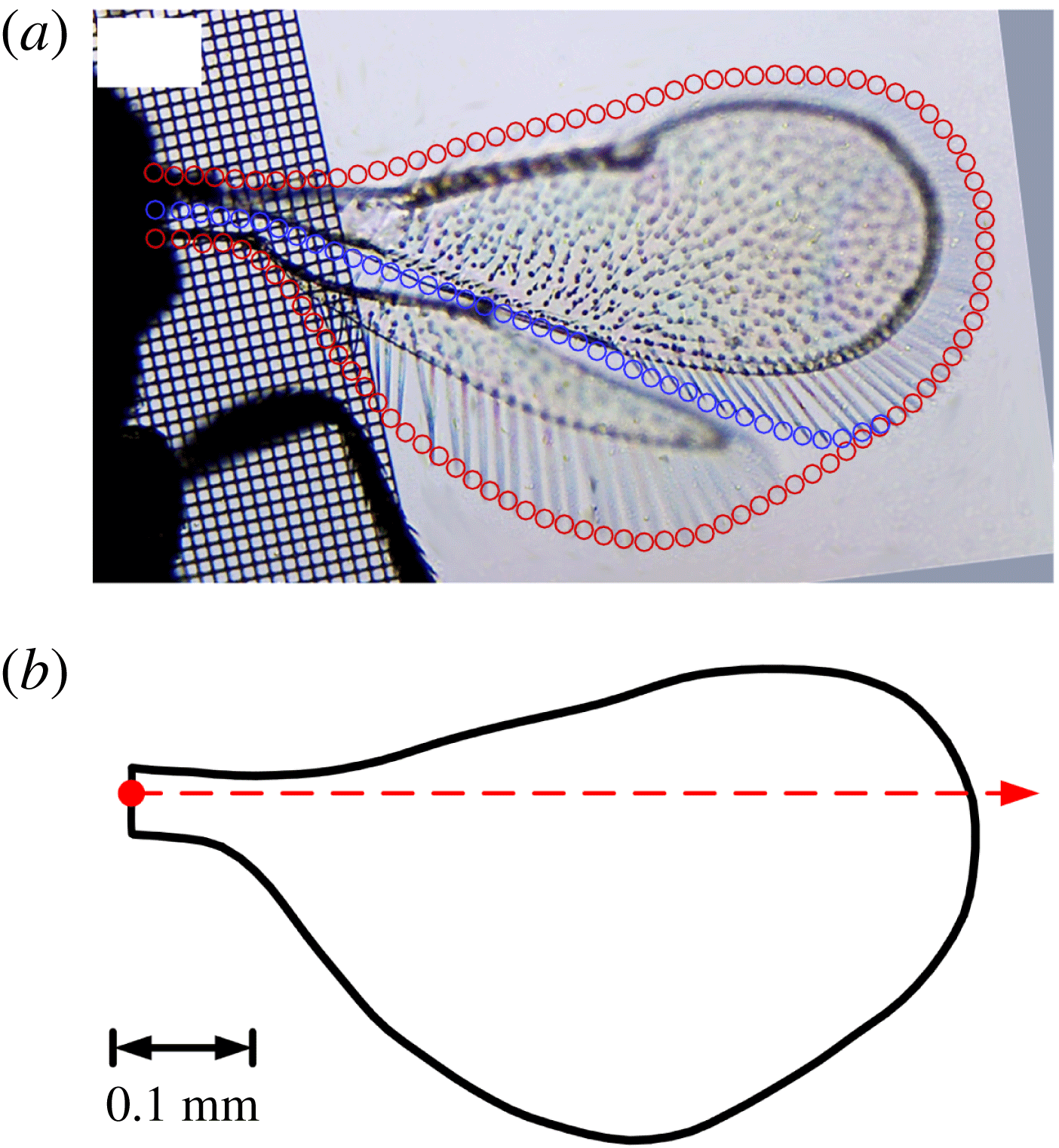
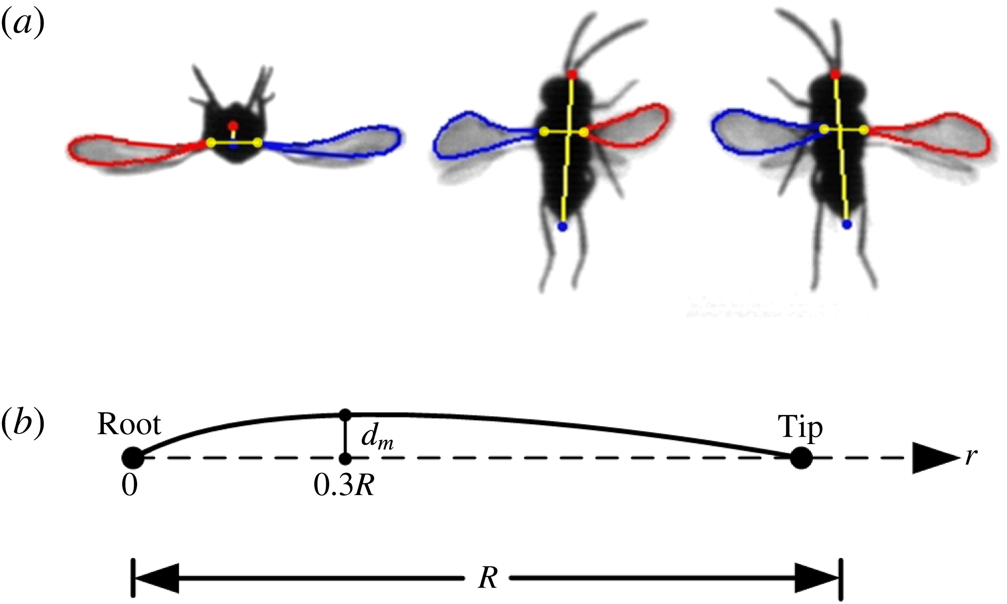
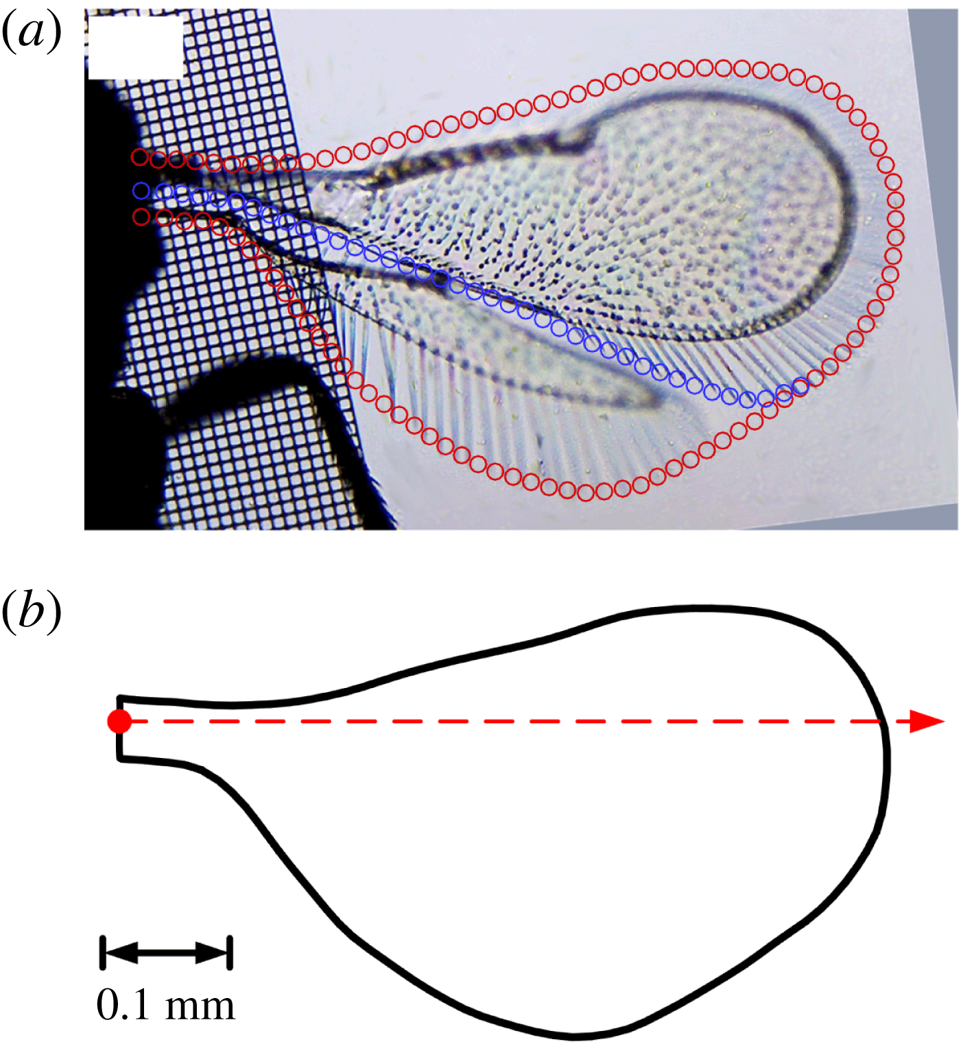
In the present study, the linked fore- and hindwings were modelled as a single wing; but the forewing could rotate relative to the hindwing around the ‘leading edge’ of the hindwing, which happened during the ‘fling’. The wing of E. formosa consists of the membrane and the brim of marginal hairs (figure 2 a), but here the hairs that line the wing are modelled as an extension of the membranous wing, i.e. the planform of the model wing is similar to that of a wing consisting of the membrane and the brim of marginal hairs (figure 2 b). The effects and limitations of these simplifying assumptions will be discussed in a later section (§ 7). The section thickness of the model wing is 3 % of the local chord length and the leading and trailing edges are rounded. The body shape is given by fitting ellipses to the body in the video images.
(a) Wing planform of an Encarsia formosa, extracted from microscope images. Blue circles indicate the boundary between fore- and hindwings. (b) The planform of the model wing used in computations. The red dot indicates the wing base and the dashed line indicates the axis of pitch rotation.
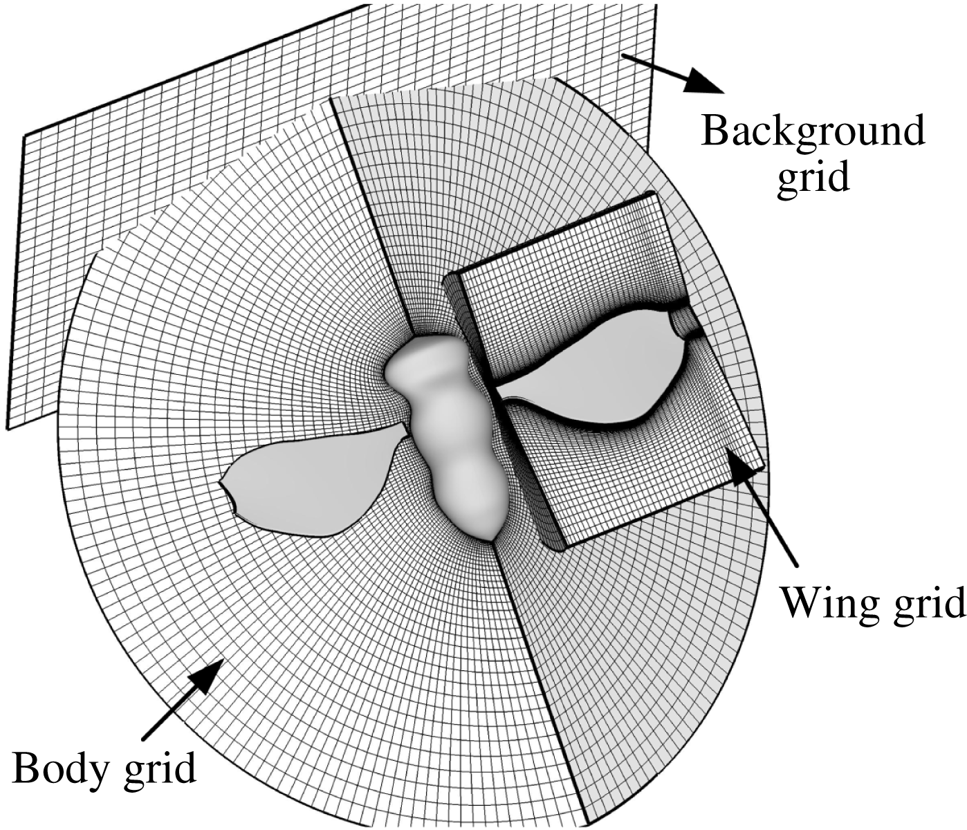
Portions of computational grids.

The equations were solved over moving overset grids because there are relative movements between the left and right wings and between the body and wing. There was a body-fitted curvilinear grid for each of the wings and the body and a background Cartesian grid which extends to the far-field boundary of the domain (figure 3). In the calculation process, the wing grid was regenerated in every time step because of the spanwise bending deformation and the rotation of the forewing relative to the hindwing during the ‘fling’. The computational method is the same as that used in several previous studies of our group (Sun & Yu Reference Sun and Yu2003, Reference Sun and Yu2006; Du & Sun Reference Du and Sun2012) and only an outline of the method is given here. The algorithm is based on the method of artificial compressibility. It was first developed by Rogers, Kwak & Kiris (Reference Rogers, Kwak and Kiris1991) for a single grid, and then extended by Rogers & Pulliam (Reference Rogers and Pulliam1994) to overset grids. The time derivatives of the momentum equations are differenced using a second-order, three-point backward difference formula. To solve the time discretized momentum equations for a divergence-free velocity at a new time level, a pseudo-time level is introduced into the equations and a pseudo-time derivative of pressure divided by an artificial compressibility constant is introduced into the continuity equation. The resulting system of equations is iterated in pseudo-time until the pseudo-time derivative of pressure approaches zero; thus, the divergence of the velocity at the new time level approaches zero. The derivatives of the viscous fluxes in the momentum equation are approximated using second-order central differences. For the derivatives of convective fluxes, upwind differencing based on the flux-difference splitting technique is used. A third-order upwind differencing is used at the interior points and a second-order upwind differencing is used at points next to boundaries. With overset grids, the solution method for a single grid is applied to each of the wing grid and the background grid, and data are interpolated from one grid to another at the inter-grid boundary points using tri-linear interpolation. Details of this algorithm can be found in Rogers et al. (Reference Rogers, Kwak and Kiris1991) and Rogers & Pulliam (Reference Rogers and Pulliam1994). For the far-field boundary conditions, at the inflow boundary, the velocity components are specified according to relative velocity at the boundary while pressure is extrapolated from the interior; at the outflow boundary, pressure is set equal to the static pressure of the still air and the velocity is extrapolated from the interior. On the wing surfaces, impermeable wall and no-slip boundary conditions are applied, and the pressure on the boundary is obtained through the normal component of the momentum equation written in the moving coordinate system. The background Cartesian grid was generated algebraically. The wing grid (O–H type) and body grid (O–O type) were generated using a Poisson solver which was based on the work of Hilgenstock (Reference Hilgenstock, Sengupta, Hauster, Eiseman and Thompson1988). The grids will be further described in § 4.1, as will be the analysis of the convergence of solutions.
3 Measured wing kinematics
Flights in eight wasps were filmed; they are denoted as EF1, EF2, EF3, EF4, EF5, EF6, EF7 and EF8, respectively. Figure 4 shows the sequences of the flight of one of the wasps (EF5); the original video sequences for the insect is presented as supplementary movies 1–3, available at https://doi.org/10.1017/jfm.2018.668.
Video sequences of a Encarsia formosa at near-hovering; three camera views are shown. Times noted are ms from the instant when the rowing starts. For complete video sequences, see supplementary movies 1–3.

In describing the wing kinematics of the wasps, a method similar to that given by Ellington (Reference Ellington1984b
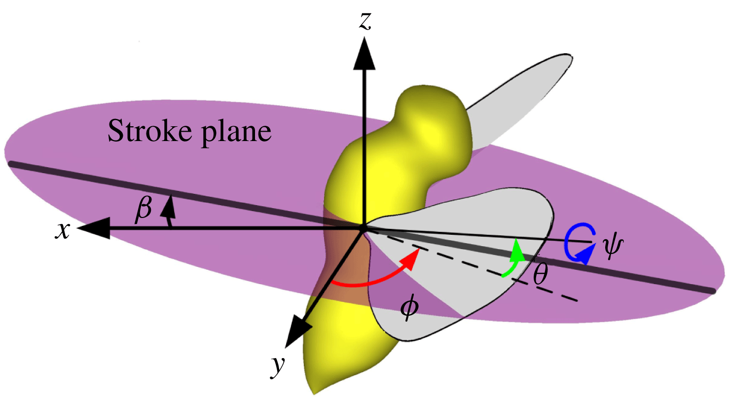
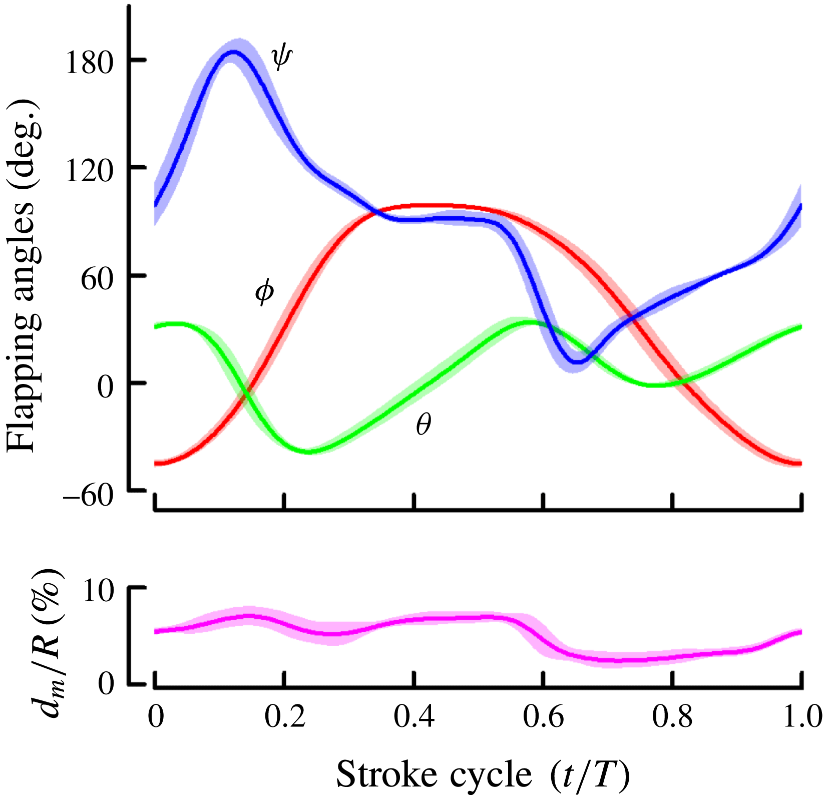
) was used. For each insect, data of six wingbeat cycles were processed. In each cycle, when the wings were at the foremost and rearmost positions, the wing-tip points were projected onto the plane of symmetry of the insect. A linear regression line of the projections was then determined. The plane which is parallel to the above line and passes the wing base is defined as the stroke plane (figure 5). Let (
 $x,y,z$
) be a reference frame with origin at the wing base, the
 $x$
axis being horizontal and pointing backward, the
 $z$
axis being vertical and pointing upward and the
 $y$
axis pointing sideward (figure 5). The orientation of a wing relative to the stroke plane can be determined by three Euler angles (figure 5):
 $\unicode[STIX]{x1D711}$
, positional angle of wing (in the stroke plane);
 $\unicode[STIX]{x1D713}$
, pitch angle;
 $\unicode[STIX]{x1D703}$
, deviation angle.
 $\unicode[STIX]{x1D6FD}$
is the stroke-plane angle.
Reference frame and Euler angles defining the wing kinematics.

Measured Euler angles and the maximum bending displacement (
 $d_{m}/R$
) from one individual, EF1 (mean
 $\pm$
s.d.;
 $n=6$
wingbeats).
 $T$
, stroke period;
 $R$
, wing length.

Figure 6 gives the measured Euler angles,
 $\unicode[STIX]{x1D711}$
,
 $\unicode[STIX]{x1D713}$
and
 $\unicode[STIX]{x1D703}$
, and the spanwise bending in one wingbeat cycle in a flying E. formosa (EF1), presented as mean values
 $\pm$
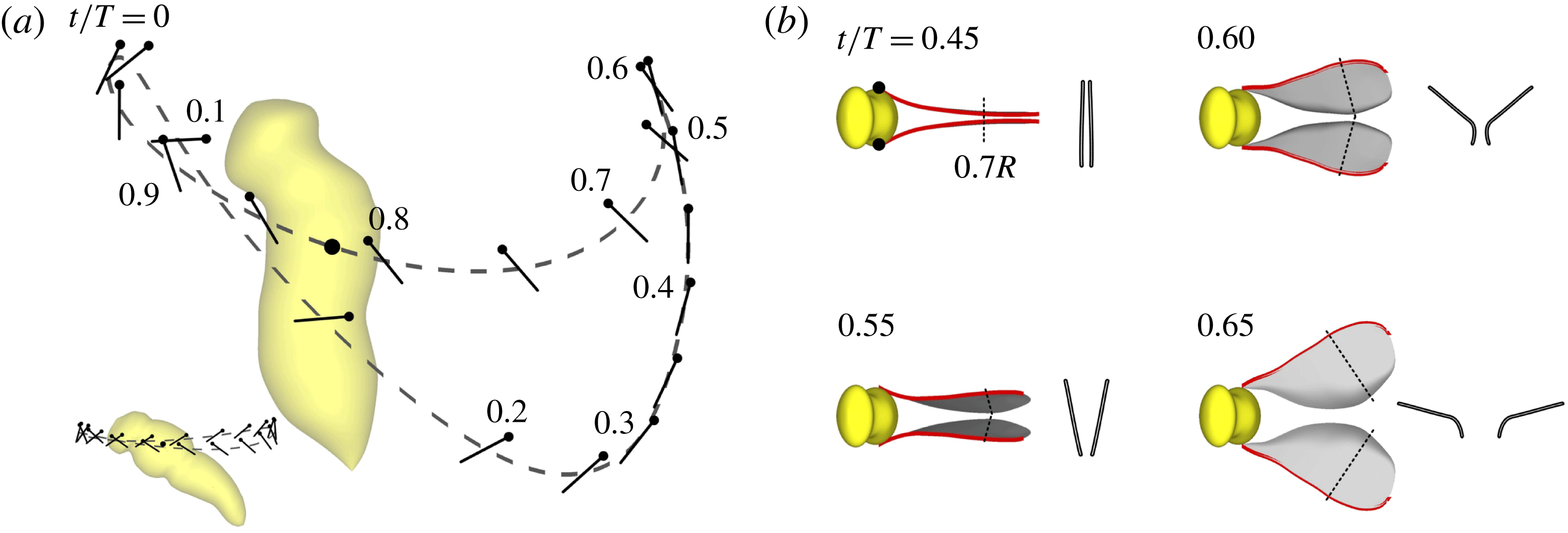
standard deviation (s.d.). Based on the data given in figure 6, the stroke diagrams of the wing motion are plotted and shown in figure 7. Larger insects in normal hover flight sweep their wings back and forth horizontally (inset, figure 7
a; Ellington Reference Ellington1984b
). For the tiny wasp, the mid-portion of the forward sweep is similar to that in normal hovering; however, towards the end of the forward sweep, the wings are swung upwards to a higher position. Then the wings move fast downward and backward with the wing surface approximately horizontal, the motion resembles that of the stroking oars of a boat or the fins of a fish swimming upwards. We thus see that the backward sweep of the wasp is very different from that of larger insects in normal hovering. Near the end of the backward sweep, the wings ‘clap’ and move vertically upwards until the wing tips reach the level of the head (figure 7
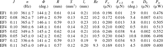
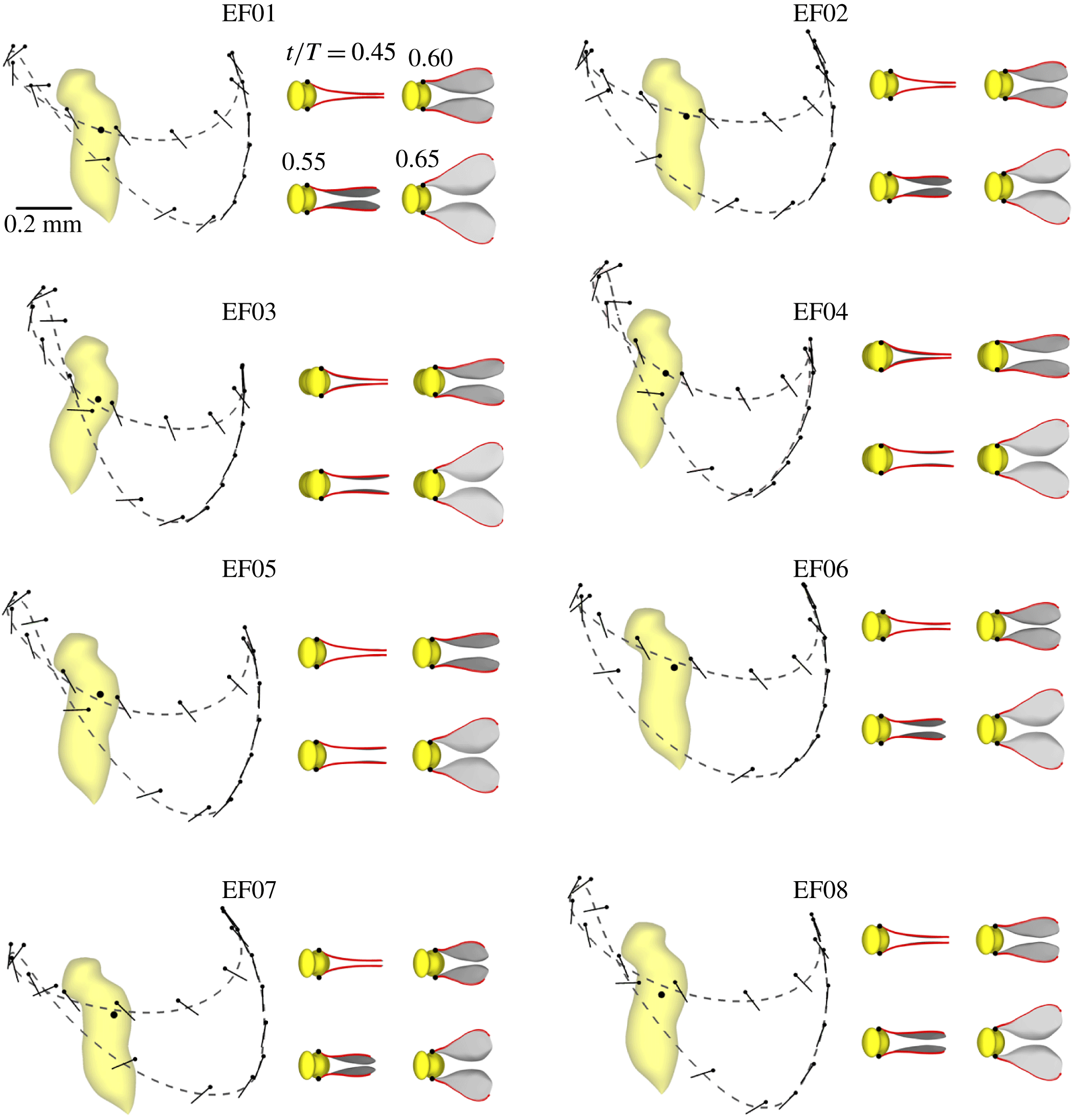
a,b), then the wings ‘fling’ open. This is the ‘clap’ and ‘fling’ described previously by Weis-Fogh (Reference Weis-Fogh1973). Wing motions of another seven individuals (table 1, supplementary movies 1–3) were measured. Most of the insects filmed were in slow ascending flight (e.g. EF1, movie 1) and their advance ratio
 $J$
(the velocity of body divided by the mean wing-tip speed) ranged from 0.02 to 0.12 (table 1). The one with
 $J=0.02$
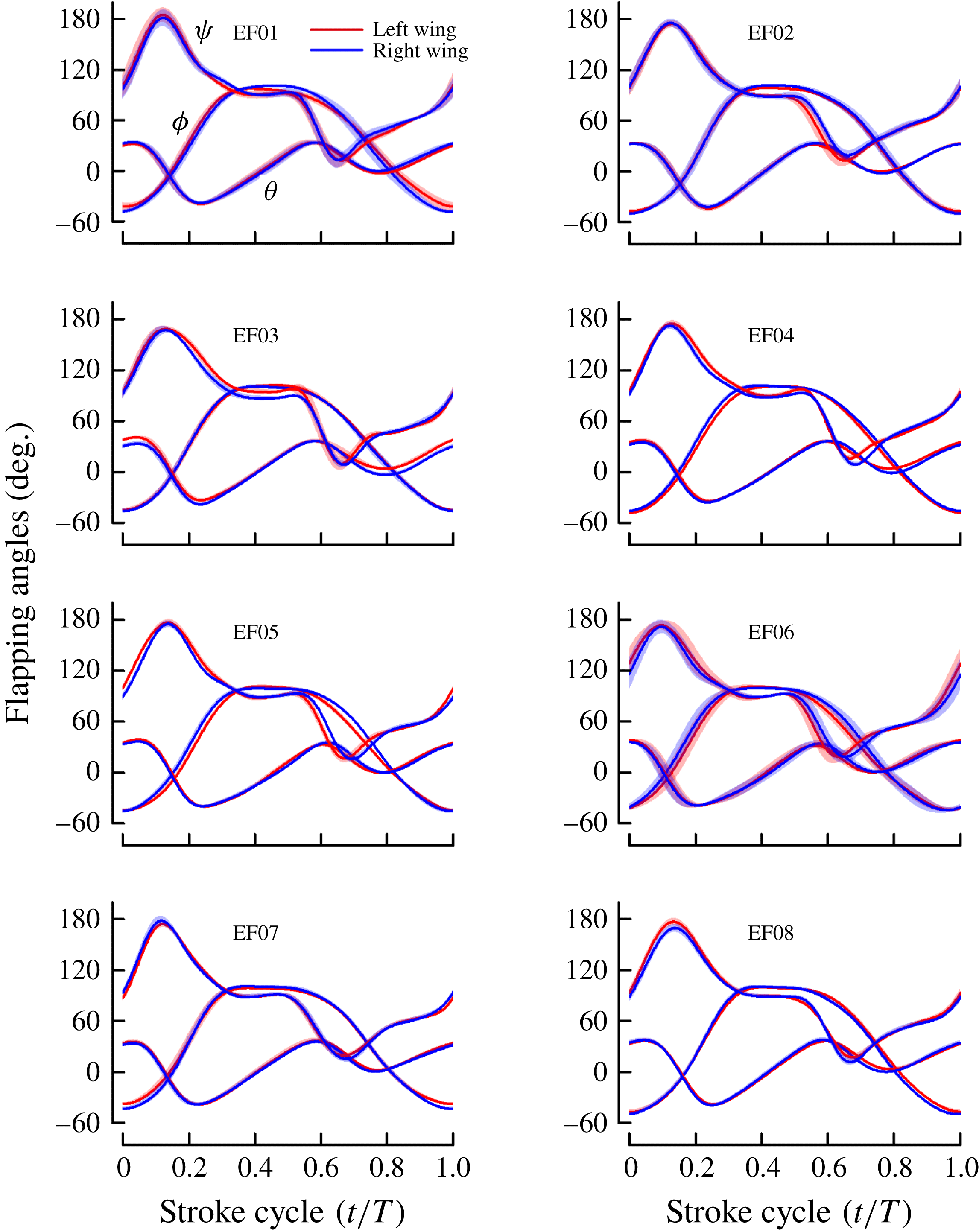
(EF5, movie 3) can be considered to be in ‘true’ hovering. Note that all the insects have approximately the same wing kinematic pattern (see figures 20–22 in appendix B).
(a) Stroke diagram shows the wing motion of Encarsia formosa (the inset shows the wing motion of a dronefly, a larger insect). The dashed curve indicates the wing-tip trajectory (projected onto the
 $x$
–
 $z$
plane); black lines indicate the orientation of the wing at 20 temporally equidistant points, with dots marking the leading edge; the black dot defines the wing-root location on the insect body. (b) Wing motion at dorsal stroke reversal, showing the Weis-Fogh ‘clap and fling’.
 $R$
, wing length.

Other morphological data of the wasps required for carrying out the analysis were also measured in the experiment, or computed on the basis of the measured data. The data included (table 1): the wing length (
 $R$
), the area of one wing (
 $S$
) and the distance between the two wing roots (
 $l_{r}$
); the radius of the second moment of wing area or radius of gyration (
 $r_{2}$
) is
 $0.64R$
for the eight insects. The weight of the insect could not be measured due to the limitation of the accuracy and measuring range of our balance.
Flight parameters for the eight Encarsia formosa, denoted as EF1–EF8.
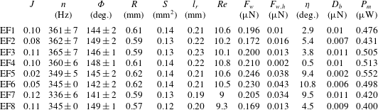
 $J$
is the advance ratio, defined as the velocity of body motion divided by the mean wing-tip speed; small
 $J$
indicates that the insects are at near-hovering.
 $n$
and
 $\unicode[STIX]{x1D6F7}$
are the stroke frequency and amplitude, respectively (mean
 $\pm$
s.d.).
 $R$
, wing length;
 $S$
, area of wing;
 $l_{r}$
, the distance between the left and right wing roots;
 $Re$
, Reynolds number;
 $F_{w}$
and
 $\unicode[STIX]{x1D702}$
, magnitude and angle from the vertical of the computed cycle-mean force vector of the wings, respectively;
 $F_{w,h}$
, the cycle-mean horizontal force of the wings;
 $D_{b}$
, body drag;
 $P_{m}$
, cycle-mean power.
4 Flows and aerodynamic-force mechanisms
To assess how the weight-supporting force is generated by the special wing motions, in this section, the flow and forces on the wings were computed and analysed.
4.1 Code validation and grid test
The flow solver had been tested by unsteady aerodynamic forces measured by translating (Meng & Sun Reference Meng and Sun2013) and rotating (Sun & Yu Reference Sun and Yu2006) model insect wings. These tests showed that the unsteady aerodynamic forces computed by the present solver agreed well with the experimental measurements. But these tests were for cases of higher Reynolds number (
 $Re$
above 200). Here we further test the solver at Reynolds numbers (
 $Re\sim 10$
) identical to the wasp flight. First, we made a conceptual test for a single, flapping wing at
 $Re=10$
(the flapping motion is an idealized flapping motion often used in insect flight study, given by Dickinson et al.
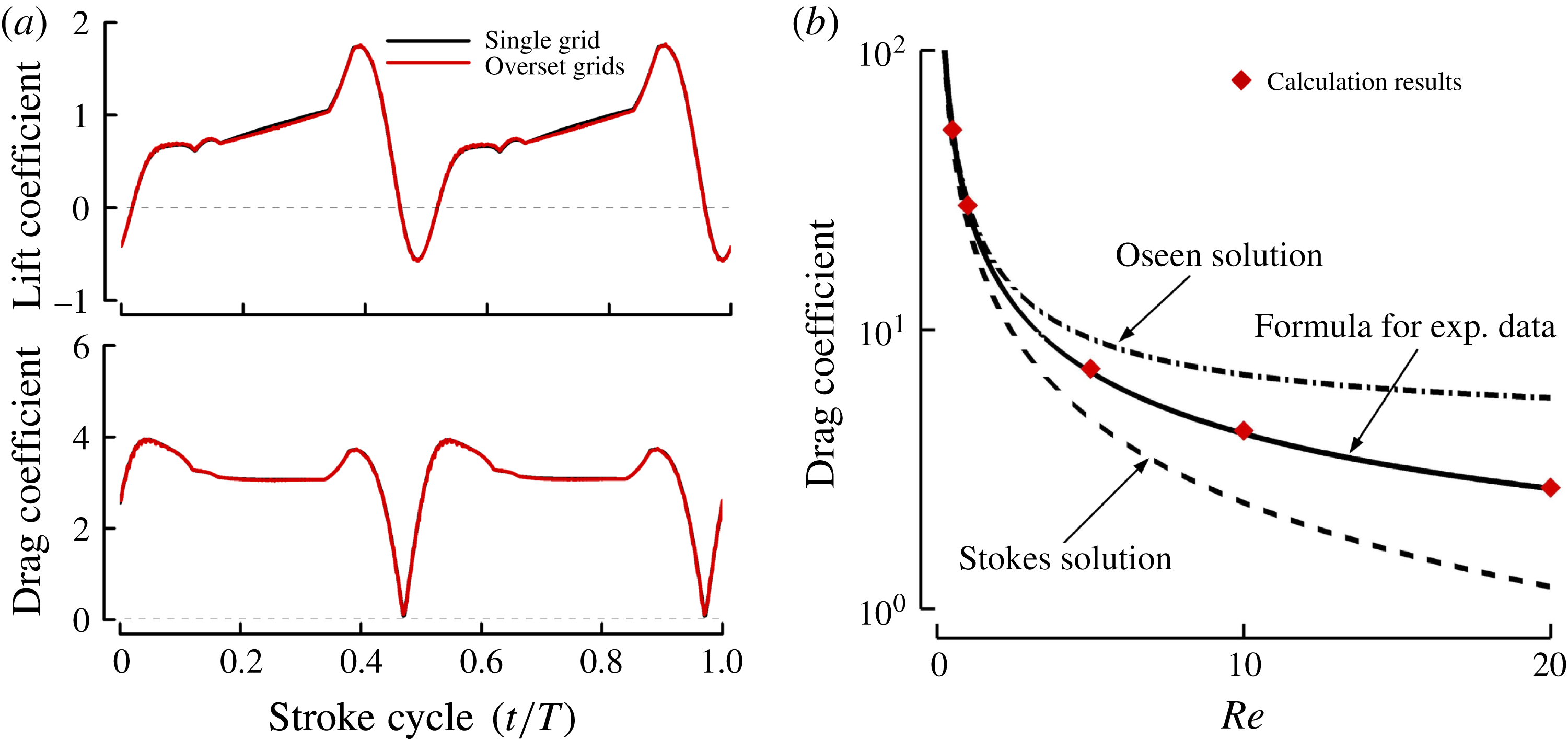
Reference Dickinson, Lehmann and Sane1999). We computed the flow first using the single grid, and then computed the flow using the multi-block, overset grids. Since the physical problem is the same in the two computations, the results should be the same. This can be a test on the multi-block, overset solver. Figure 8(a) shows the comparison in the lift and drag coefficients (
 $C_{L}$
and
 $C_{D}$
) between the two computations. There is very good agreement between these two sets of results, showing that the multi-block, overset Navier–Stokes solver works well at
 $Re$
around 10.
(a) Lift and drag coefficients of a single wing flapping at
 $Re=10$
computed using a single grid, compared with those computed using the multi-block, overset grids. (b) The calculated drag coefficient of a sphere at
 $Re=0.5{-}20$
, compared with the theoretical results and experimental data.

To further validate the low-
 $Re$
simulation, we computed the flows around a sphere at
 $Re=0.5{-}20$
, for which there exist Stokes or Oseen solutions and accurate experiment data (White Reference White1991). Figure 8(b) compares the computed drag coefficient with the theoretical and experimental data. The difference between the computed results and the data is less than 2 %.
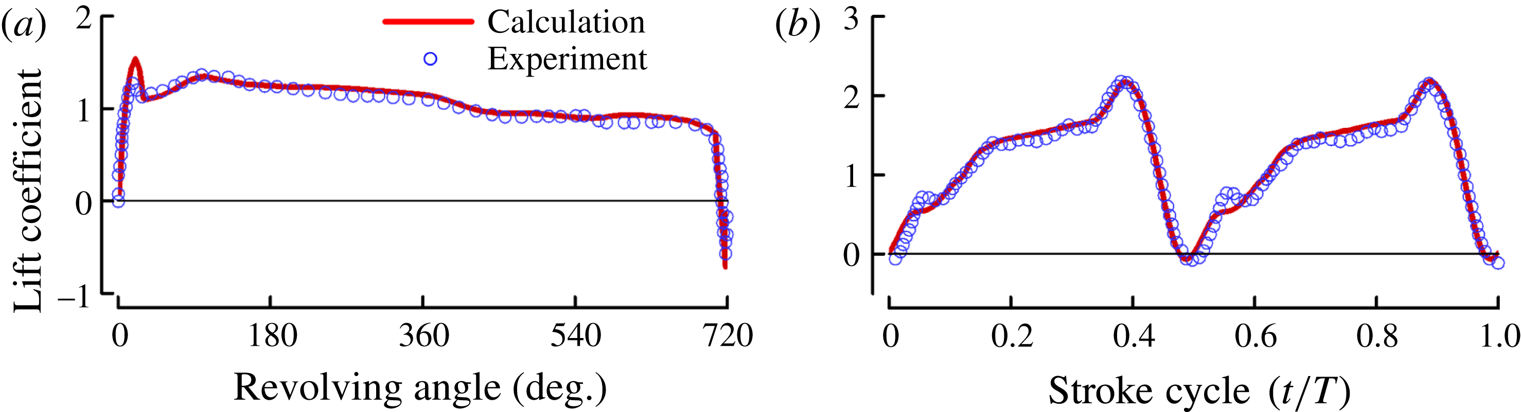
As mentioned above, the flow solver was tested by measured data of translating and rotating wings. Recently, lift coefficient (
 $C_{L}$
) was measured for model insect wings in flapping motion at
 $Re=180$
(Han, Chang & Han Reference Han, Chang and Han2016) and in revolving motion with an acceleration phase, a constant-speed phase and a deceleration phase at
 $Re=500$
(Manar & Jones Reference Manar and Jones2014). Here we make a further test of the solver using these experiment data. As seen in figure 9, the computed
 $C_{L}$
agrees very well with the measured data.
Comparison between the calculated and measured lift coefficients on a rectangular wing in revolving motion with an acceleration phase, a constant-speed phase and a deceleration phase (
 $Re=500$
) (a), and on a model fruitfly wing in flapping motion (
 $Re=180$
) (b).

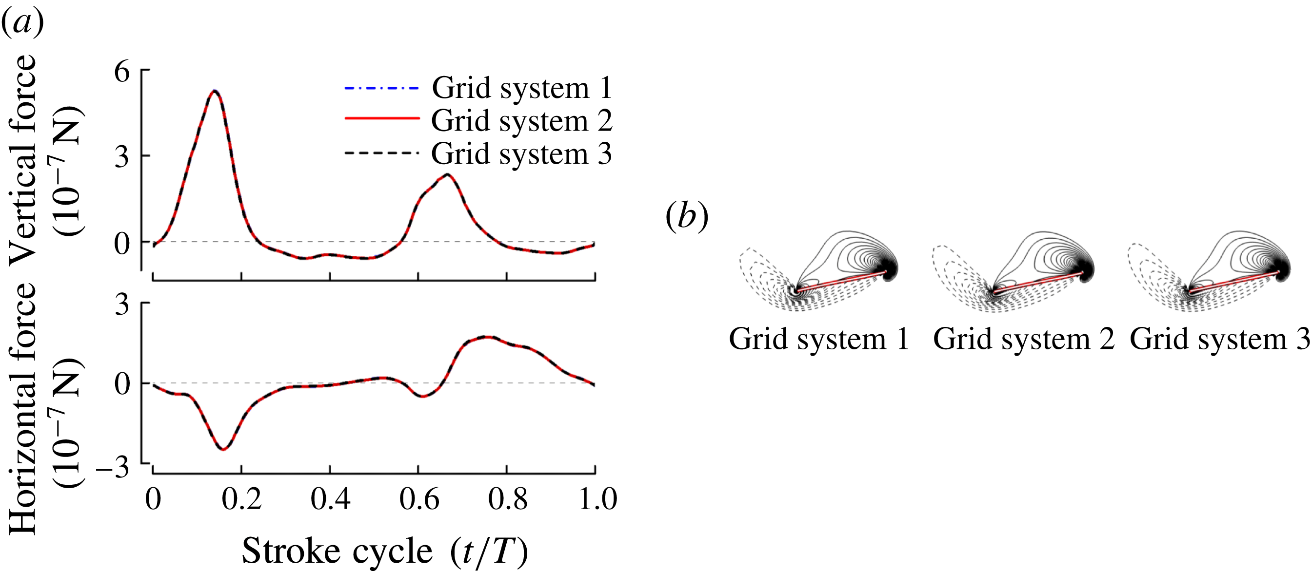
Before proceeding to compute the flows, grid resolution tests were conducted to ensure that the flow calculation was grid independent. Three grid systems were considered. For grid system 1, the wing grid had dimensions
 $41\times 61\times 43$
in the normal direction, around the wing, and in the spanwise direction, respectively (first layer grid thickness was
 $0.0015c$
); the body grid had dimensions
 $66\times 51\times 35$
along the body, in the azimuthal direction and in the normal direction, respectively; the background grid had dimensions
 $81\times 81\times 81$
in the
 $x$
,
 $y$
and
 $z$
directions, respectively. For grid system 2, the corresponding grid dimensions were
 $61\times 91\times 65$
,
 $99\times 77\times 53$
and
 $121\times 121\times 121$
(
 $0.001c$
). For grid system 3, the corresponding grid dimensions were
 $91\times 135\times 96$
,
 $149\times 118\times 80$
and
 $181\times 181\times 181$
(
 $0.00067c$
). For all three grid systems, the outer boundary of the background grid was
 $20c$
from the wing root; the grid points of the background grid concentrated in the near field of the wings where its grid density was approximately the same as that of the outer part of the body grid. The typical cell size in the near wake, where vortices from a stroke may interact with the wing in the subsequent strokes, was less than
 $0.038c$
,
 $0.061c$
and
 $0.1c$
for grid systems 3, 2 and 1, respectively. The aerodynamic forces and vorticity patterns computed from three grid systems are shown in figure 10 (the wings started to flap in a quiescent fluid, and after about three cycles the flow became periodical). It is observed that there is almost no difference between the forces calculated by the three grid systems (figure 10
a). The first grid refinement produces a little change in the vorticity plot, and the second grid refinement produces almost no change (figure 10
b). Calculations were also conducted using a larger computational domain. The domain was enlarged by adding more grid points to the outside of the background grid of grid system 2 (the outer boundary of the background grid of grid system 2 was increased from
 $20c$
to
 $40c$
). The calculated results showed that there was no need to put the outer boundary further than that of grid system 2. The non-dimensional time step was 0.02 (non-dimensionalized by
 $c/U$
). The effect of time step value was studied and it was found that a numerical solution effectively independent of the time step was achieved if the time step value was
 ${\leqslant}0.02$
. From the above discussion, it was concluded that grid system 2 and time step 0.02 were appropriate for the calculation.
Grid resolution test. (a) Time courses of the vertical and horizontal forces of the wings in one cycle, calculated with three grid systems. (b) The corresponding non-dimensional spanwise vorticity contours at section
 $0.7R$
at
 $t/T=0.14$
; the magnitude of the non-dimensional vorticity at the outer contour is 3 and the contour interval is 1.

4.2 Aerodynamic forces
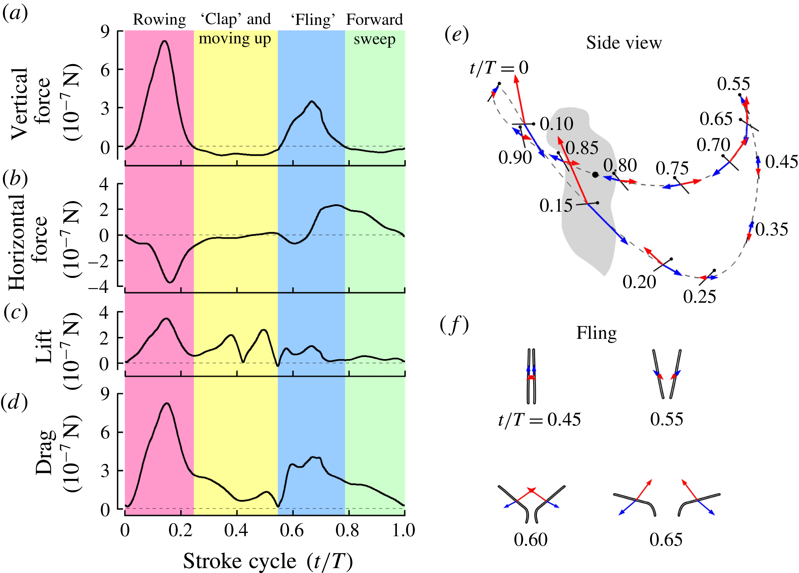
In the present study, the vertical and horizontal components of the total aerodynamic force of a wing are referred to as vertical force and horizontal force, respectively. Because the wing does not translate in the horizontal plane, the vertical force is not the lift of the wing and the horizontal force is not the drag. The velocity at the radius of gyration (
 $r_{2}$
) of the wing is used to represent the velocity of the wing (figure 11
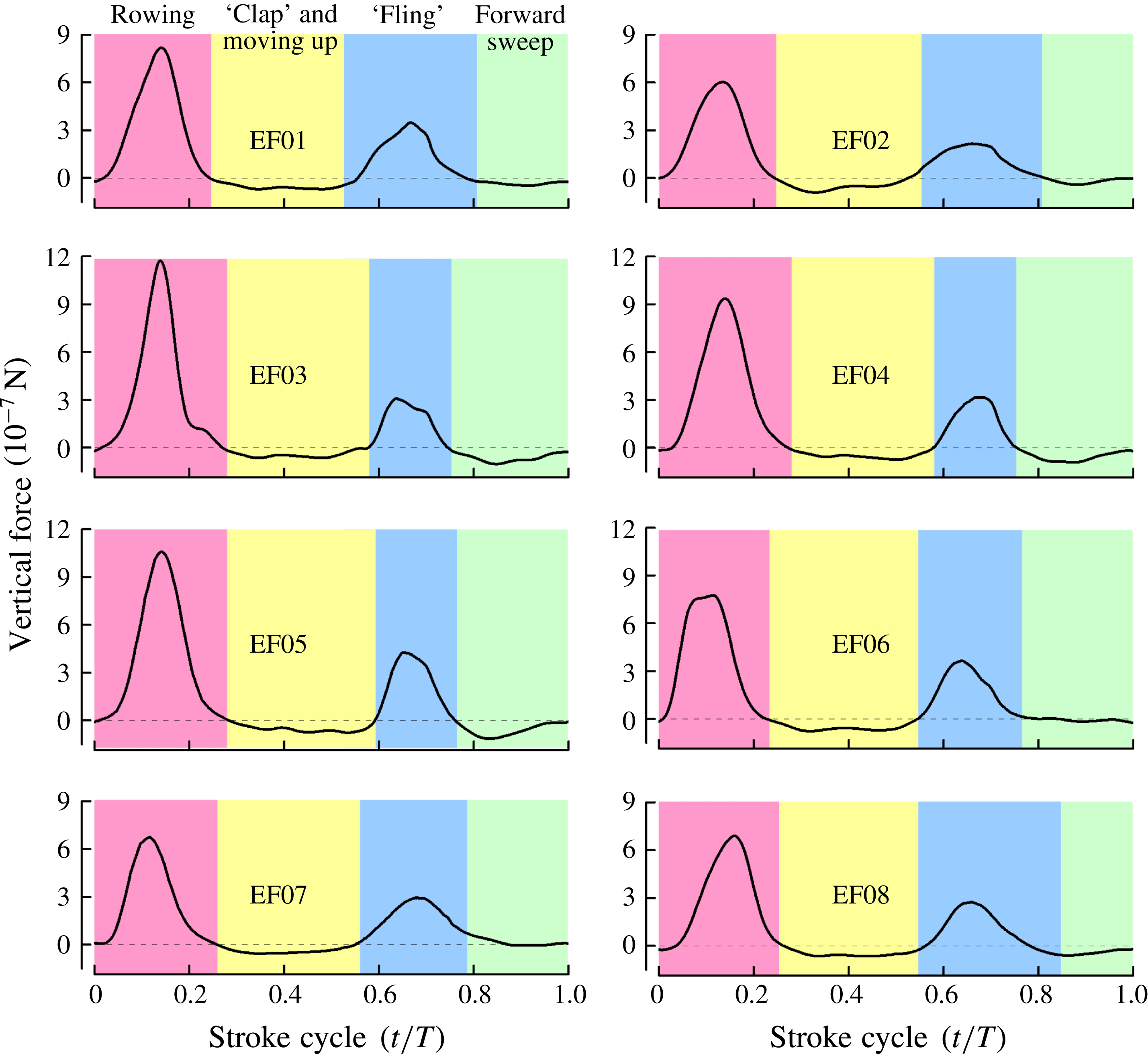
e). Lift and drag are defined as the components of the total aerodynamic force that are perpendicular and parallel to the velocity of the wing, respectively. Figure 11(a–d) gives the time histories of the computed aerodynamic forces of a wing in one cycle for EF1 (results for the other seven individuals are given in appendix B, see figure 23). Because the computed forces show great consistency for the eight individuals, we analyse the results of EF1 (figure 11) as an example. As seen from the figure, a large vertical-force peak is produced during the rowing (figure 11
a,
 $t/T\approx 0{-}0.2$
) and another smaller one during the ‘fling’ (figure 11
a,
 $t/T\approx 0.55{-}0.7$
); the other parts of the cycle do not produce any positive vertical force. From the data in figure 11(a), it is calculated that the rowing contributes 70 % of the total vertical force and the ‘fling’ the other 30 %. The rowing produces a forward pointing horizontal force and the ‘fling’ and the subsequent forward sweeping produces a backward pointing horizontal force (figure 11
b), and the two approximately cancel, as required for hovering and ascending flight.
Aerodynamic forces. (a–d) Vertical force, horizontal force, lift and drag of a wing. (e) Diagram showing the wing position, velocity vector and force vector at various times in one stroke cycle (side view). (f) Back view of the wing in ‘fling’ motion, represented by the wing section at
 $0.7R$
, and the corresponding velocity vector and force vector. Blue arrow, velocity; red arrow, force.

As mentioned, the insects are in hovering or very slow ascending flight. Thus the computed mean force vector of the wings should be vertical. As seen in table 1, the mean force vector is very close to being vertical: its horizontal component (
 $F_{w,h}$
) is small and the angle between the force vector and the vertical (
 $\unicode[STIX]{x1D702}$
) is less than
 $6^{\circ }$
for five of the eight wasps and approximately
 $10^{\circ }$
for the other three. The magnitude of the mean force vector of the wings (
 $F_{w}$
) is shown in table 1. When in slow ascending flight, there is a small drag on the body (the computed body drag,
 $D_{b}$
, is also given in table 1). The value of (
 $F_{w}$
–
 $D_{b}$
) should be equal to the weight of the insect. As mentioned above, we could not measure the weight of the insects in our experiment. Weis-Fogh (Reference Weis-Fogh1973) measured the weight of ten wasps of the same species as those in our experiment (E. Formosa) and gave the average weight of the insects. Since the wasps in our experiment and those in Weis-Fogh’s experiment are the same species, they are geometrically similar. Thus we can make an indirect comparison here. For the insects in Weis-Fogh’s experiment, the average wing length was 0.62 mm, the average wing-tip speed was
 $1.17~\text{m}~\text{s}^{-1}$
and the average weight was
 $0.245~\unicode[STIX]{x03BC}\text{N}$
. For the eight insects in our experiment, the average wing length is 0.6 mm and the average wing-tip speed is
 $0.1075~\text{m}~\text{s}^{-1}$
. Assuming that the aerodynamic force is proportional to the wing area (or the square of the wing length) and to the square of wing-tip speed, the average weight of the insects in our experiment can be estimated as
 $$\begin{eqnarray}\left({\textstyle \frac{0.6}{0.62}}\right)^{2}\times \left({\textstyle \frac{1.075}{1.17}}\right)^{2}\times 0.245~\unicode[STIX]{x03BC}\text{N}=0.194~\unicode[STIX]{x03BC}\text{N}.\end{eqnarray}$$
The computed average
 $F_{w}$
–
 $D_{b}$
for the eight insects is
 $0.196~\unicode[STIX]{x03BC}\text{N}$
, in good agreement with the above estimated average weight (
 $0.194~\unicode[STIX]{x03BC}\text{N}$
).
4.3 Aerodynamic-force mechanisms
The vertical and horizontal forces of a wing come from its lift and drag. The rowing produces a large drag and a much smaller lift (figure 11
c,d). Therefore, the large vertical force by the rowing is mainly from the drag of the wing (approximately 70 % of the vertical force during the rowing period is contributed by the drag). In this period, the wing is in a transient motion (velocity increases from zero at
 $t/T=0$
to a large value at
 $t/T=0.15$
and then decreases to a small value at
 $t/T\approx 0.2$
) and the angle of attack is rather large, between
 $46^{\circ }$
and
 $65^{\circ }$
(figure 11
e). The transient motion and force here are very similar to those of an oar of a boat. Let us examine how the large drag is produced.
Since the wing is in fast acceleration (
 $t/T=0{-}t/T\approx 0.15$
) and deceleration (
 $t/T\approx 0.15{-}t/T\approx 0.2$
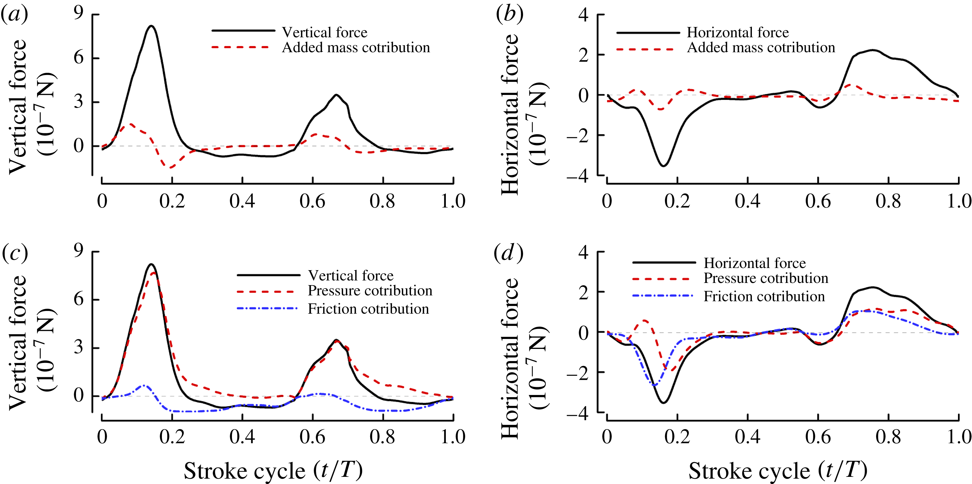
), we first look at the role of added mass. Howe (Reference Howe1989, Reference Howe1995) made an analysis of the force exerted on a rigid body in unsteady motion in a uniform incompressible viscous fluid, and showed that the force on the body is the summation of three parts. The first part is caused by the acceleration of the body and the expression of this part is identical to the added-mass force obtained by solving the potential flow of no free vorticity, and the second and third parts are due to the free vorticity in the wake and the viscous skin friction, respectively. His results show that the added mass of a rigid body moving in an incompressible fluid can be computed by solving a separate potential flow. Our group recently developed a code for computing the added mass force of flapping wings (Liu & Sun Reference Liu and Sun2018). Using the code we calculated the added-mass force during the rowing period and the results are shown in figure 12(a,b). It is seen that the added-mass forces are relatively small. The large drag must be produced by other mechanisms.
(a,b) Added-mass contributions to the vertical and horizontal forces. (c,d) The contributions of the pressure- and friction-based components to the vertical and horizontal forces.

Figure 12(c,d) shows the contributions of the pressure- and friction-based components to the vertical and horizontal forces. It is seen that the large vertical force or the large drag of the wing is mainly contributed by the pressure-based component (figure 12
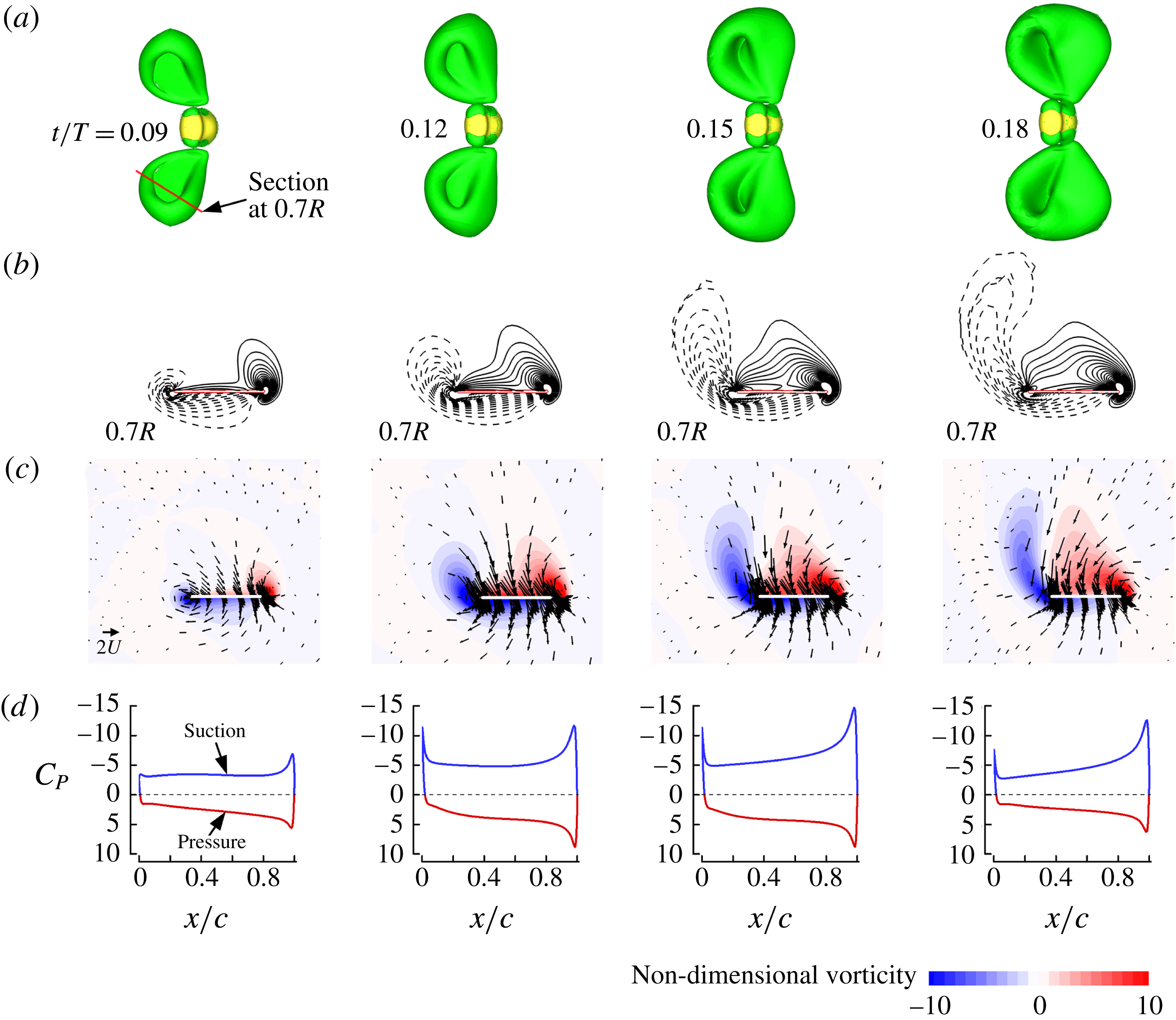
c). Let us investigate how the large pressure-based force is generated. Flow field data in this period are shown in figure 13. The fluid is pushed downwards by the ‘lower’ wing surface and sucked downwards by the ‘upper’ wing surface (figure 13
c). Strong vortices are shed at the leading and trailing edges (figure 13
a,b). The pushing results in a large pressure on the lower surface of the wing and the induced velocity of the leading-edge vortex (LEV) and trailing-edge vortex (TEV) results in a large suction pressure on the upper surface of the wing (figure 13
d), giving the large drag or vertical force. Note that for the tiny insects here, both the LEV and TEV are used in enhancing the aerodynamic force production, unlike the cases for larger insects whose
 $Re$
is larger than 100, where LEV dominates the enhancement of aerodynamic force production. We thus see that the large pressure force that gives the large drag or vertical force is generated by the unsteady effect similar to that of starting flow of a plate started in its normal direction.
Flow fields and surface pressure distributions during the rowing period. (a) Iso-vorticity surface plots (top view) at
 $t/T=0.09$
, 0.12, 0.15 and 0.18 (in this and other plots of iso-vorticity surfaces, the magnitude of the non-dimensional vorticity is 2). Vorticity is non-dimensionalized by
 $U/c$
. (b) Non-dimensional spanwise vorticity contours at section
 $0.7R$
; solid and dashed lines denote the anticlockwise and clockwise vorticity, respectively. The magnitude of the non-dimensional vorticity at the outer contour is 1 and the contour interval is 1. (c) Non-dimensional velocity vector plot at section
 $0.7R$
. (d) Non-dimensional surface pressure distributions at section
 $0.7R$
. Non-dimensional pressure,
 $C_{P}$
, is defined as
 $(p-p_{\infty })/0.5\unicode[STIX]{x1D70C}U^{2}$
.

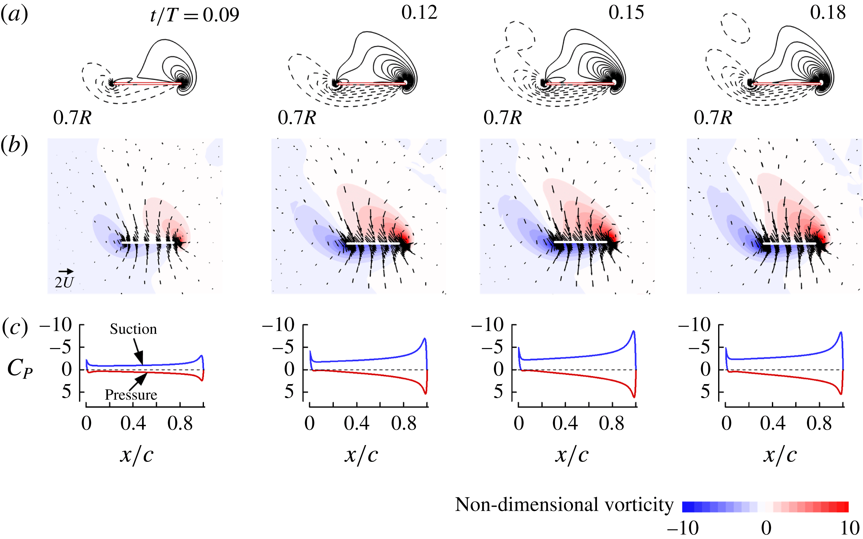
To further show the unsteady effect of the transient motion on the aerodynamic forces in the rowing period, we computed the corresponding steady flows of the wing, i.e. at each time point in the rowing period, we use the instantaneous speed and angle of attack of the wing at that time to compute a steady-state flow. For example, at
 $t/T=0.09$
in figure 13, the wing’s tip speed and angle of attack were known; we let the wing move (revolve) at the given tip speed and angle of attack until the flow reached steady state (after the wing revolved for more than one revolution, the flow became steady), thus we obtain the corresponding steady flow and force for this time point. We do the same for other time points,
 $t/T=0.12$
, 0.15 and 0.18 and so on. The steady-state results are shown in figure 14. It is seen that in the steady-state cases, the vortices shed at the leading and trailing edges are much weaker and the pressure on the lower surface and the suction on the upper surface are much smaller than the corresponding ones in the transient motion (comparing results in figure 14 with those in figure 13). The reason for the LEV and TEV in the unsteady case being much stronger than those in the steady-state case is as follows. The wing in the unsteady case is similar to a plate in starting motion in its normal direction, in which vorticity shed at the edges of the plate could accumulate to a large amount behind the plate. We computed the vertical force from the steady-state case and it is 45 % less than that produced by the unsteady (rowing) motion.

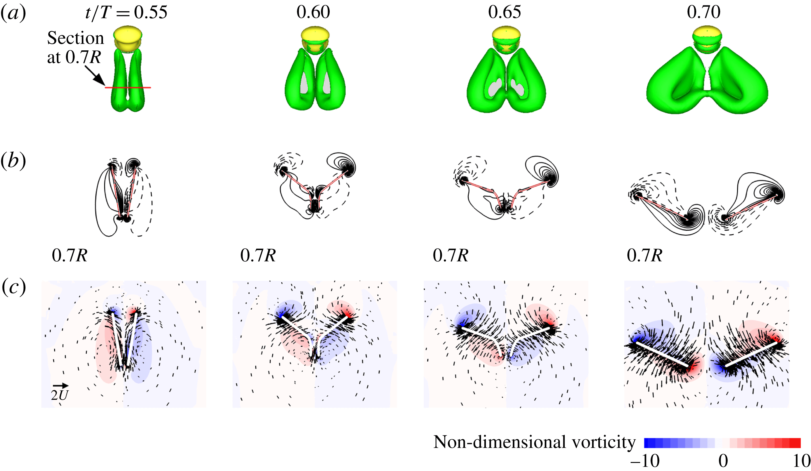
Next, let us look at the vertical-force peak during the ‘fling’. It is also due to the large drag on the wing (see figure 11 a,d,f). The production mechanism of the large drag has been explained in detail by many previous studies (Spedding & Maxworthy Reference Spedding and Maxworthy1986; Sun & Yu Reference Sun and Yu2003; Miller & Peskin Reference Miller and Peskin2005; Arora et al. Reference Arora, Gupta, Sanghi, Aono and Shyy2014). Flow field data during the ‘fling’ are shown in figure 15. As pointed out in previous studies (Spedding & Maxworthy Reference Spedding and Maxworthy1986; Sun & Yu Reference Sun and Yu2003; Miller & Peskin Reference Miller and Peskin2005), the mechanism of the vertical-force peak during the ‘fling’ is that the opening of the wing pair generates a vortex ring containing a strong downward jet (see figure 15 a,c) in a very short period, or a large fluid impulse, resulting in the large force.
Flow fields during the ‘fling’ period. (a) Iso-vorticity surface plots (top view) at
 $t/T=0.55$
, 0.60, 0.65 and 0.70. (b) Non-dimensional spanwise vorticity contours at section
 $0.7R$
. Solid and dashed lines denote the anticlockwise and clockwise vorticity, respectively. (c) Non-dimensional velocity vector plot at section
 $0.7R$
.

5 Aerodynamic power
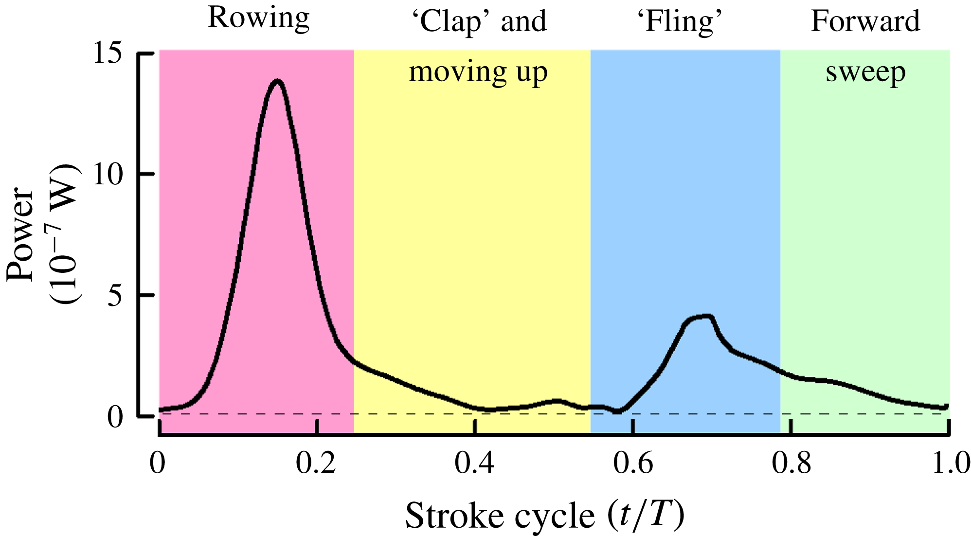
From the computed aerodynamic force and the wing motion data, the power used by the wing to generate the forces was calculated and shown in figure 16. It is seen that power in the rowing and the ‘fling’ periods is large, as expected.
Aerodynamic power of a wing in one wingbeat cycle.

From data in figures 11(a) and 16, the mean vertical force and mean power are calculated as
 $0.196~\unicode[STIX]{x03BC}\text{N}$
and
 $0.476~\unicode[STIX]{x03BC}\text{W}$
respectively, giving a value of
 $2.43~\text{W}$
per Newton lifted
 $(\text{W}~\text{N}^{-1})$
(referred to as specific power). Weis-Fogh (Reference Weis-Fogh, Wu, Brokaw and Brennen1975) found that large (10 kg) or small (
 $1~\unicode[STIX]{x03BC}\text{g}$
) animals derive mechanical power from the same type of muscle and the specific power that an animal can supply is independent of size, and it can be up to
 $6~\text{W}~\text{N}^{-1}$
. The tiny wasp’s required power (
 $2.4~\text{W}~\text{N}^{-1}$
) is far below this limit. Power is consumed by a wing when it moves against the drag. Airplanes, birds and larger insects use lift to support the weight and the specific power is made small by having a large lift-to-drag ratio (e.g. 10). For the tiny wasp, drag is used to support the weight and the ‘lift-to-drag’ ratio is 1, far from being large. Why do the tiny wasps still have a small specific power? Let
 $D$
be the mean drag of one wing and it is equal to half of the weight. The mean angular speed of the wing is proportional to the wingbeat frequency
 $n$
and the torque due to the drag to
 $RD$
(
 $R$
, wing length). Then the power is proportional to
 $nRD$
and the specific power to
 $nR$
. Since
 $n$
varies with size according to
 $R^{-0.68}$
(Dudley Reference Dudley2002), the specific power is proportional to
 $R^{0.32}$
. As insect size decreases, the specific power would decrease, answering the above question.
6 Why special wing movements and drag principle must be used
Using drag to produce the weight-supporting vertical force has been shown previously in some insects. Wang (Reference Wang2004) and Sun & Lan (Reference Sun and Lan2004) found that a hovering dragonfly, with inclined stroke plane and asymmetric flapping, used drag to support approximately three-quarters of its weight. For a hovering hoverfly with inclined stroke plane and asymmetric flapping, approximately 45 % of the vertical force was contributed by the drag (Zhu & Sun Reference Zhu and Sun2017). These insects (dragonfly and hoverfly) can also hover with a horizontal stroke plane (Ellington Reference Ellington1984b
; Wakeling & Ellington Reference Wakeling and Ellington1997); in this case the vertical force is produced using the lift principle only. That is, dragonflies and hoverflies can choose to use lift or drag to produce the weight-supporting force. However, the tiny wasps must use the unusual wing motions and the drag principle to fly. To understand the reasons for this, we simplified its wing kinematics to that employed by the larger insects: wings sweeping back and forth in a horizontal plane (figure 7
a, inset), but kept
 $Re$
unchanged and re-computed the flows and forces. In the computation, the stroke amplitude (
 $144^{\circ }$
), frequency (361 Hz) and Reynolds number (10.6) are the same as those of the tiny wasp. The angle of attack at mid-stroke (
 $\unicode[STIX]{x1D6FC}_{m}$
) is set as
 $35^{\circ }$
–
 $55^{\circ }$
(as will be seen below, when
 $\unicode[STIX]{x1D6FC}_{m}$
is larger than
 $40^{\circ }$
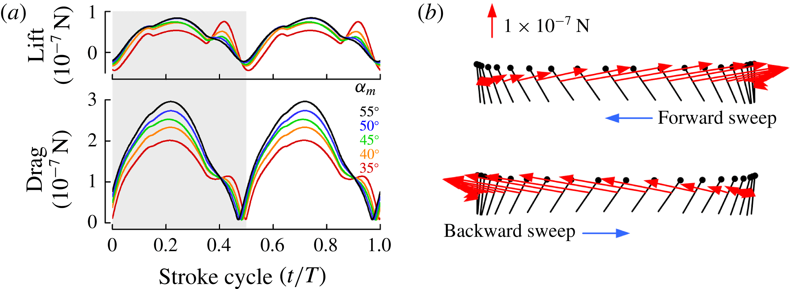
, the lift will change little and drag becomes larger and larger). The computed results are shown in figure 17.
Aerodynamic forces produced if the tiny wasp used the same wing kinematics as that of the large insects. (a) Lift (vertical force) and drag. Grey shading represents the forward stroke. (b) Diagram of wing motion indicating magnitude and orientation of force vectors (
 $\unicode[STIX]{x1D6FC}_{m}=50^{\circ }$
). Black lines indicate the instantaneous position of the wing at 40 temporally equidistant points during a stroke cycle. Small circles mark the leading edge. Time moves right to left during forward stroke, left to right during backward stroke. Red vectors indicate instantaneous forces.

Now the vertical force is simply the lift and the drag only contributes to the horizontal force. As seen from figure 17(a), the wing produces a very small lift but a much larger drag; the force vector on the wing is approximately backward pointing in the forward sweep and forward pointing in the backward sweep (figure 17
b). The mean lift, or mean vertical force, is only approximately
 $1/3$
of that produced by using the real wing kinematics.
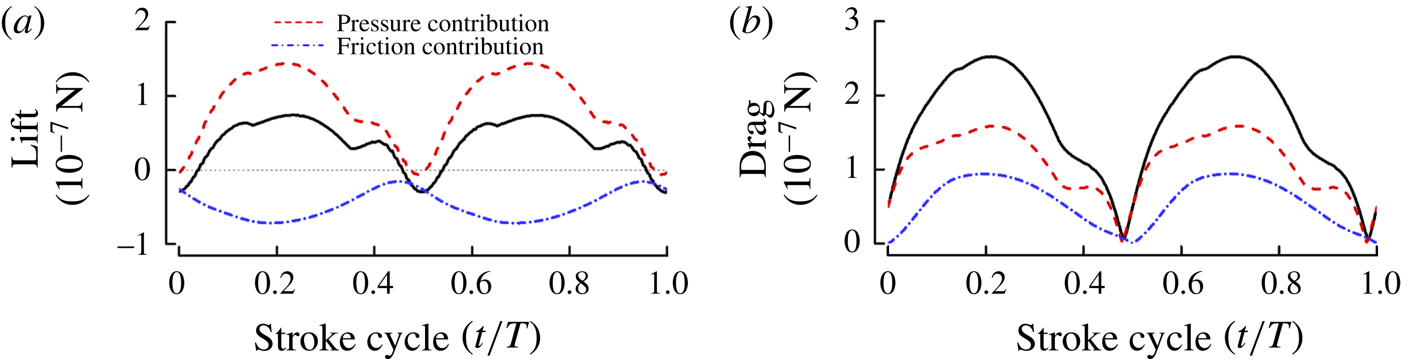
To explain why the lift is very small while the drag is very large, we plot the contributions to the lift and drag from the pressure and the viscous stress on the wing surface (figure 18). It is seen that, at this low
 $Re$
(10.6), the viscous stress on the wing surface is rather large; and it makes a large negative contribution to the lift and a large positive contribution to the drag, resulting in the very small lift and the much larger drag.
Contributions to the lift and drag from the pressure and the viscous stress on the wing surface (
 $\unicode[STIX]{x1D6FC}_{m}=45^{\circ }$
).

The above results show that the tiny wasps cannot use the wing kinematics commonly employed by the larger insects (wings sweeping back and forth in a horizontal plane) to generate the required vertical force. This explains why they use the special flapping motions, rowing and ‘fling’: these motions enable them to overcome the problem of insufficient lift at the very small Reynolds numbers encountered by the commonly used flapping kinematics.
Finally, let us discuss using the drag principle for flight. The oar of a boat is in water during the effective stroke but in air during the return stroke, so that the return stroke requires little power. For the wasp, as seen in figure 10(a), no useful vertical force is produced in the period of ‘clap’ and moving upward and neither in the period of forward sweeping. These two periods may be taken as the ‘return stroke’ where the power requirement is very small. This is indeed the case: from data in figure 16, the power required during the rowing and the ‘fling’ periods are 60 % and 21 % of the total power requirement, respectively. However, in the two ‘return periods’ (‘clap’ and moving upward; forward sweeping), the values are much smaller, only 10 % and 9 %, respectively. This is because in these two ‘return periods’ the velocity and angle of attack of the wings are small (see figure 11 e); the angle of attack in the period of ‘clap’ and moving upward is almost zero (the wing surface is almost vertical). That small insects may use a drag mechanism for flight was suggested a long time ago (Horridge Reference Horridge1956) and also recently (Jones et al. Reference Jones, Laurenza, Hedrick, Griffith and Miller2015). But people had never yet observed a very small insect in flapping flight which used drag rather than lift. Here we have observed for the first time very small insects using drag to produce the vertical force for flight, and explained how the drag and the net vertical force were produced.
7 On the study limitation
A forewing or hindwing of E. formosa consists of a membranous part and the brim of marginal hairs (figure 2 a) and the two wings move as a single wing. In our model wing used in the computation, the brim hair part is assumed to be an extension of the membranous part and the fore- and hindwings are modelled as a single membranous wing.
Sunada et al. (Reference Sunada, Takashima, Hattori, Yasuda and Kawachi2002) measured the lift and drag forces on a bristled model wing and a solid-plate wing of the same shape. Different wing motion patterns were considered: azimuthally rotating (revolving) at a constant angular speed and at a constant angular acceleration; translating at a constant speed and at a constant acceleration. Among these motions, the revolving motions at constant speed and at constant acceleration are the major components of the flapping motion of an insect wing. They showed that at
 $Re$
around 10, the aerodynamic forces acting on the bristled model wing were a little smaller than those on the solid wing. The ratio of aerodynamic forces (lift and drag) between the bristled wing and the solid wing is between 0.85 and 1 for revolving at constant speed (see figure 4 in Sunada et al.
Reference Sunada, Takashima, Hattori, Yasuda and Kawachi2002) and between 0.7 and 1 for revolving at constant acceleration (see figure 8 in Sunada et al.
Reference Sunada, Takashima, Hattori, Yasuda and Kawachi2002). Let us assume that the ratio is 0.85 (the mean value of 0.7 and 1); that is, the aerodynamic forces produced by the bristled wing are approximately 15 % smaller than those by the membranous wing. The lift and drag are a result of the pressure-based force and viscous friction-based force on the wing. Because of the low
 $Re$
, there can be little flow through the gap between the bristles (Ellington Reference Ellington, Wu, Brokaw and Brennen1975) and the bristled wing might produce a similar momentum or pressure-based lift and drag to those of the membranous wing; whereas, because the bristled wing has a much lower solid wing area, its viscous friction-based lift and drag might have a relatively large difference compared to those of the membranous wing. Therefore, one may expect that the viscous friction-based forces play an important role in causing the differences in the aerodynamic-force production between the bristled and membranous wings.
From the above experimental data of Sunada et al. (Reference Sunada, Takashima, Hattori, Yasuda and Kawachi2002), modelling a bristled wing as a membranous wing may cause an error of approximately 15 % in the aerodynamic-force calculation. For E. formosa in the present study, the wing is not completely bristled (approximately 62 % of the wing area is membranous and the bristles are at the brim of the membranous part, accounting for approximately 38 % of the wing area). Furthermore, the distance between the bristles in the E. formosa wing (approximately
 $0.007R$
, where
 $R$
is the wing length) is much smaller than that in the bristled model wing in Sunada et al.’s (Reference Sunada, Takashima, Hattori, Yasuda and Kawachi2002) experiment (
 $0.018R$
). Taking these two points into account, the error in our aerodynamic-force calculations should be substantially smaller than 15 %. Nevertheless this is a limitation of the present study.
8 Conclusion
The smallest insects are of very large number and of great ecological and biological significance. For these insects, the effect of air viscosity is so large that lift-generation mechanisms used by their larger counterparts become ineffective. How the weight-supporting force is generated is unknown. Our wing kinematics measurement and flow analysis in the tiny wasp Encarsia formosa in hovering flight answer the above question. The tiny insects perform two unusual wing motions. One is ‘rowing’: the wings move fast downward and backward, like stroking oars. The other is the previously discovered Weis-Fogh ‘fling’. The rowing produces 70 % of the required vertical force and the Weis-Fogh ‘fling’ the other 30 %. The oaring wing mainly produces an approximately up-pointing drag, resulting in the vertical force. Because each oaring produces a starting flow, the drag is unsteady in nature and much greater than that in steady motion at the same velocities and angles of attack. Furthermore, our computation shows that if the tiny wasps employed the usual wing kinematics of the larger insects (flapping back and forth in a horizontal plane), vertical force produced would be only
 $1/3$
of that by the real wing kinematics; i.e. they must use the special wing movements to overcome the problem of large viscous effects encountered by the commonly used flapping kinematics. We have observed for the first time very small insects using drag to support their weight and we explain how a net vertical force is generated when drag principle is applied.
Acknowledgements
This research was supported by grants from the National Natural Science Foundation of China (11832004, 11721202). X.C. was supported by the Academic Excellence Foundation of BUAA for PhD students.
Supplementary movies
Supplementary movies are available at https://doi.org/10.1017/jfm.2018.668.
Appendix A. Method of wing kinematics measurement
Kinematics extraction and wing bending definition. (a) Extraction of body and wing kinematics. (b) Definition of the spanwise bending of wing.
 $d_{m}$
, maximum bending displacement, assumed to be at
 $0.3R$
.

The method used to extract the 3-D body and wing kinematics from the filmed data was a modification of that used in several previous works of our group (Liu & Sun Reference Liu and Sun2008; Mou et al. Reference Mou, Liu and Sun2011). First the original method is outlined (see Mou et al. (Reference Mou, Liu and Sun2011) for its detailed description). The body and wings were represented by models: the model of a wing was a flat-plate wing having the outline obtained by scanning the cut-off wing of the insect and the model of the body was two lines perpendicular to each other, which were the line connecting the head and the end of the abdomen and the line connecting the two wing hinges (figure 19 a). An interactive graphic user interface was developed using MATLAB (MATLAB v. 7.1, MathWorks Inc., Natick, MA, USA) to extract the 3-D body and wing positions from the frames recorded by the three cameras. The positions and orientations of the models of the body and wings were adjusted until the best overlap between a model image and the displayed frame was achieved in three views, and at this point the positions and orientations of these models were taken as the positions and orientations of the body and the wings; the fitting process was done manually.
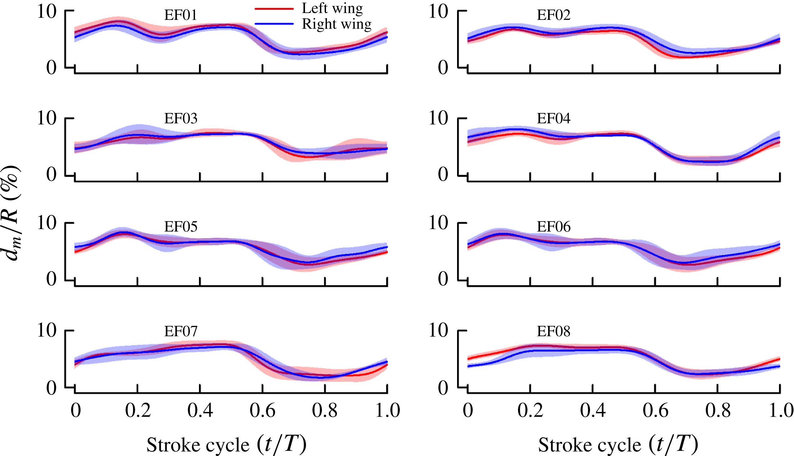
In the above method, the model of the wing was a rigid flat plate. But for E. formosa, considerable spanwise bending of the ‘stalked’ wing exists, as observed from the snapshots in figure 4. The bending is relatively large during the rowing and the ‘clap-and-fling’ periods and smaller in the rest of the cycle. We dealt with this problem by making the following changes to the above method. The model of the wing was no longer a rigid flat-plate wing, but a plate wing that has spanwise bending (figure 19
b). Based on the observations, it was assumed that the maximum bending displacement,
 $d_{m}(t)$
, was at 30 % of wing length from the wing root. We approximate the bending displacement between
 $r/R=0$
and
 $r/R=0.3$
by one quadratic curve and that between
 $r/R=0.3$
and
 $r/R=1$
by another, thus the bending displacement is determined when
 $d_{m}(t)$
determined.
 $d_{m}(t)$
is determined in process of matching the model image and the displayed frame. With the above modification, in addition to the three Euler angles,
 $d_{m}(t)$
was also measured.
Appendix B. Measured wing kinematics and computed forces for all eight individuals
Wing kinematics for each of the eight wasps. Three flapping angles of wing (mean
 $\pm$
s.d.). For details, see the legend of figure 6. Time courses of the angles among the eight individuals are similar.

Stroke diagrams for each of the eight wasps. For each individual, left, wing-tip trajectory and orientation of wing at 20 temporally equidistant points; right, wing motion at dorsal stroke reversal, showing the ‘clap and fling’. For details, see the legend of figure 7. Kinematic patterns for the eight individuals are approximately the same.

Spanwise bending of each of the eight wasps. The maximum bending displacement
 $d_{m}/R$
(mean
 $\pm$
s.d.) in one stroke cycle. For details, see the legend of figure 6.

Vertical force for each of the eight wasps. The computed forces show great consistency for the eight individuals.