





1. Introduction
Convective flows of electrically conducting fluids influenced by magnetic fields are readily found throughout nature and in many industrial processes. Examples of such naturally occurring flows arise in the study of stellar convection zones and liquid metal planetary cores (Jones Reference Jones2011), with industrial applications including liquid metal batteries, casting, semi-conductor crystal growth and liquid-metal blanket cooling systems for nuclear fusion reactors (Davidson Reference Davidson1999). Despite the physical relevance of such systems, our understanding of magnetoconvection has been limited because of numerous experimental and computational difficulties (Schumacher Reference Schumacher2022). Experiments, which often require the use of opaque liquid metals, are unable to use commonly available optical imaging techniques, and numerical studies usually require substantial computational resources. To mitigate these challenges, either greatly simplified systems are used or the simulations are evolved only for short times. The result is that little is known about the often slowly evolving spatiotemporal dynamics in such systems, especially at high magnetic field strengths.
The onset of magnetoconvection with a vertical magnetic field has been studied in a few isolated scenarios through linear stability analysis: in the case of an infinite/periodic plane layer by Chandrasekhar (Reference Chandrasekhar1961), and in the case of a semi-infinite sidewall by Busse (Reference Busse2008). Such analysis reveals that the sidewalls in a system are responsible for the onset of convection at high relative magnetic field strengths (typically characterised by the Hartmann number  ${\textit {Ha}}$), particularly relevant to industrial processes that often occur in closed vessels. Indeed, an analytic–numerical hybrid analysis performed by Houchens, Witkowski & Walker (Reference Houchens, Witkowski and Walker2002) for the special case of a cylindrical geometry showed that sidewalls were responsible for the onset, producing thin convective layers attached to these sidewalls, commonly referred to as wall modes. However, knowledge about nonlinear effects and the later stages of transition to turbulence is still limited.
Wall modes in quasistatic magnetoconvection with a vertical magnetic field were first examined in the full system numerically by Liu, Krasnov & Schumacher (Reference Liu, Krasnov and Schumacher2018), who conducted direct numerical simulations in a box of aspect ratio  $\varGamma =4$ up to
 ${\textit {Ha}}=2000$ with no-slip boundaries, confirming that onset occurred below the linear stability threshold of the infinite plane layer. Wall modes were seen to have a three-dimensional spatial structure, featuring thin rolls pressed against the sidewalls in an alternating pattern of positive and negative rotation. Thus, between each set of rolls lay alternating structures with positive and negative vertical velocities which were additionally seen to have protrusions that extended into the bulk of the domain. At increased levels of thermal driving (typically characterised by the Rayleigh number
 ${\textit {Ra}}$), more chaotic cellular-style regimes were observed, although details of the transition were not characterised.
Although hints of wall modes were present in the experiments of Cioni, Chaumat & Sommeria (Reference Cioni, Chaumat and Sommeria2000), wall modes were first confirmed experimentally in a cylinder by Zürner et al. (Reference Zürner, Schindler, Vogt, Eckert and Schumacher2020), who additionally characterised the cellular regime more carefully, with various numbers of cells being observed at different regions of the  $({\textit {Ra}},{\textit {Ha}})$ parameter space. Further simulations in a cylinder were performed by Akhmedagaev et al. (Reference Akhmedagaev, Zikanov, Krasnov and Schumacher2020), as well as more recently by Xu, Horn & Aurnou (Reference Xu, Horn and Aurnou2023), who combined new experimental and numerical results. From the current data, it appears that the wall-mode protrusions grow with increased
 ${\textit {Ra}}$, extending towards the bulk of the domain exhibiting quasi-steady dynamics. Once the critical
 ${\textit {Ra}}$ of the bulk onset is reached, i.e. the onset in the infinite plane layer (Chandrasekhar Reference Chandrasekhar1961), the cellular regime ensues, producing a more chaotic variation in system observables such as the dimensionless heat transport (Nusselt number
 ${\textit {Nu}}$). For
 ${\textit {Ha}} < 300$ at mostly higher
 ${\textit {Ra}}$, Zürner et al. (Reference Zürner, Schindler, Vogt, Eckert and Schumacher2020) observed large-scale rolls, i.e. the large-scale circulation (LSC) that is commonly found in classical Rayleigh–Bénard convection (RBC), and thus it is assumed that at sufficiently large
 ${\textit {Ra}}$ magnetoconvection will approach more familiar solutions of RBC.
In summary, although some information about the transition to turbulence is known in magnetoconvection, many questions are still open, mostly concerning the various dynamics admissible by this system. Specifically, it is currently not well understood how the transition between steady wall mode solutions and the more chaotic cellular regime takes place, or what states potentially exist in between. In particular, it is relevant to try and characterise the series of bifurcations that occur upon increased  ${\textit {Ra}}$ in this system, and to study how heavily this depends on the relative magnetic field strength
 ${\textit {Ha}}$. To address these questions in the present study, we have performed an array of long numerical simulations in a box of aspect ratio
 $\varGamma =1$, in many instances on the order of 1000 free-fall times, to study this transition and the associated spatiotemporal dynamics.
Wall modes also occur in rotating Rayleigh–Bénard convection (RRBC). There are similarities between wall modes in magnetoconvection and in RRBC, especially near onset, where both types of wall modes have a similar two-layer structure. This is likely attributable to the extensive similarities in the linear theory between the two systems (Herrmann & Busse Reference Herrmann and Busse1993; Busse Reference Busse2008). However, a number of differences exist between the two systems in terms of their secondary instabilities and further nonlinear effects. In the rotating case, a Hopf bifurcation leads to an azimuthal precession of the wall modes (Ecke, Zhong & Knobloch Reference Ecke, Zhong and Knobloch1992), which is not seen to occur in magnetoconvection. Concerning the spatial structure, striations found in the RRBC wall modes at higher supercriticalities, as observed by Ecke, Zhang & Shishkina (Reference Ecke, Zhang and Shishkina2022), have not been found in magnetoconvection. With that being said, the two systems do exhibit similarities with regard to some nonlinear effects, such as wall-mode protrusions extending into the bulk, which are sometimes identified as plume-like jets in the rotating case. It is yet to be seen whether somewhat similar dynamics to those presented here could exist in some regimes of RRBC.
2. Formulation
We consider a three-dimensional flow of electrically conducting fluid driven by an imposed vertical temperature difference between the top and bottom of the domain, and in the presence of a vertical magnetic field  $\boldsymbol {B}=B_0 \boldsymbol {e}_z$. Under the quasistatic approximation – that is, for magnetic Reynolds number
 ${\textit {Rm}} = U\ell /\eta \ll 1$ and magnetic Prandtl number
 ${\textit {Pm}} = \nu /\eta \ll 1$, where
 $U$ and
 $\ell$ are characteristic velocity and length scales,
 $\eta$ is the magnetic diffusivity and
 $\nu$ is the kinematic viscosity – and the Oberbeck–Boussinessq approximation, the velocity field
 $\boldsymbol {u}$ and the temperature field
 $T$ evolve from suitable initial conditions according to the following equations:
 $$\begin{gather} \partial_t\boldsymbol{u} + \boldsymbol{u}\boldsymbol{\cdot}\boldsymbol{\nabla} \boldsymbol{u}+\boldsymbol{\nabla} p = \sqrt{\frac{{\textit{Pr}}}{{\textit{Ra}}}} [\nabla^2\boldsymbol{u} + {\textit{Ha}} ^2(\,\boldsymbol{j}\times\boldsymbol{e}_z)] + T\boldsymbol{e}_z, \end{gather}$$
 $$\begin{gather}\partial_t T + \boldsymbol{u}\boldsymbol{\cdot}\boldsymbol{\nabla} T = \frac{1}{\sqrt{{\textit{Ra}}{\textit{Pr}}}}\nabla^2T, \end{gather}$$
 $$\begin{gather}\boldsymbol{\nabla} \boldsymbol{\cdot} \boldsymbol{u} = 0, \quad \boldsymbol{j} =-\boldsymbol{\nabla}\phi + (\boldsymbol{u}\times\boldsymbol{e}_z), \quad \nabla^2\phi = \boldsymbol{\nabla}\boldsymbol{\cdot}(\boldsymbol{u}\times\boldsymbol{e}_z), \end{gather}$$
where  $p$ is the kinematic pressure,
 $\boldsymbol {j}$ is the electric current density,
 $\phi$ is the electric field potential and
 $\boldsymbol {e}_z$ is the unit vector that points vertically, opposed to gravity. Here, variables have been made dimensionless by using the container height
 $H$ and the free-fall velocity
 $u_f=(\alpha g H\delta T)^{1/2}$ to construct length, velocity and time scales, while the temperature difference between the bottom and top plates,
 $\delta T = T_+ - T_-$, and the applied magnetic field strength
 $B_0$ have been used to construct the dimensionless temperature and magnetic field strength, respectively. In turn, the control parameters of the governing equations (2.1) are the Rayleigh number
 ${\textit {Ra}} = {\alpha g \delta T H^3}/{\kappa \nu }$, the Prandtl number
 ${\textit {Pr}}={\nu }/{\kappa }$ and the Hartmann number
 ${\textit {Ha}}= B_0 H ({{\sigma }/{\rho \nu }})^{1/2}$, where
 $\sigma$ is the electrical conductivity,
 $\rho$ is the mass density,
 $\alpha$ is the thermal expansion coefficient,
 $g$ is the acceleration due to gravity and
 $\kappa$ is the thermal diffusivity. No-slip boundary conditions are applied to all boundaries, and constant temperatures
 $T_+$ and
 $T_-$ are applied to the bottom
 $(z=0)$ and top
 $(z=H)$ plates, respectively. The domain is equipped with adiabatic sidewalls
 $\partial T/\partial \boldsymbol {n}=0$, where
 $\boldsymbol {n}$ is the vector orthogonal to the surface, and electrically insulating boundaries
 $\partial \phi /\partial \boldsymbol {n}=0$.
These equations have been solved numerically at a range of  ${\textit {Ra}}$ and
 ${\textit {Ha}}$ for a fluid with
 ${\textit {Pr}}=0.025$ (such as the GaInSn alloy) in a cubic domain of unit aspect ratio, i.e.
 $\varGamma = L/H = W/H = 1$, where
 $L$ and
 $W$ are respectively the length and the width of the domain perpendicular to
 $\boldsymbol {e}_z$. This has been done using the direct numerical solver goldfish (Reiter, Zhang & Shishkina Reference Reiter, Zhang and Shishkina2022), which has been widely used in previous studies of convective flows. This version (Teimurazov et al. Reference Teimurazov, McCormack, Linkmann and Shishkina2023) uses a fourth-order finite-volume discretisation on staggered grids, and a third-order Runge–Kutta time marching scheme which has been extended to simulate magnetoconvective flows using a consistent and conservative scheme (Ni & Li Reference Ni and Li2012). A compromise had to be made in terms of the grid resolution, owing to the high computational cost. The flows are resolved on non-uniform grids with
 $220^2$ points in the cross-plane direction and with either 300 or 350 points in the vertical direction, which are sufficient to resolve the Hartmann, Shercliff and thermal boundary layers, with at least 5, 15 and 20 grid points, respectively, within each layer. The ratio between the largest finite-volume cell length and the Kolmogorov scale, calculated from the mean dissipation rate, is less than 3 in the worst case, and less than 2 in the vast majority of simulations. Changes in grid resolution were not seen to qualitatively change the observed dynamics. Most simulations were initialised from a lower-resolution simulation with
 ${\textit {Ha}}=0$, with the magnetic field strength being progressively increased, although a few of the solutions were continued from one another. We try here to broadly classify the states that exist in this flow, rather than tracking a detailed route to turbulence.
3. Numerical results
3.1. Comparison to linear stability theory
A number of linear stability results are relevant for the system under consideration. Each of these results is derived from perturbations to a static flow field  $\boldsymbol {u}=0$ and linear temperature profile. The dispersion relation for the case of an infinite plane layer/periodic sidewalls and no-slip upper and lower boundaries was derived by Chandrasekhar (Reference Chandrasekhar1961). To apply this result to our cube
 $(\varGamma =1)$, we minimise the dispersion relation for each value of
 ${\textit {Ha}}$ over the discrete horizontal wavenumbers admitted by the domain. This results in the critical Rayleigh number in the bulk,
 ${\textit {Ra}}_{c,b}$, which is plotted in figure 1. At the values of
 ${\textit {Ha}}$ considered, the wavelength of the most unstable mode in the infinite plane layer is smaller than the size of our domain, and continues to decrease with
 ${\textit {Ha}}$. Thus, the bulk onset is seen to be nearly identical in our closed geometry compared to the infinite plane layer.
The parameter space studied, given by the Hartmann number ( ${\textit {Ha}}$) and Rayleigh number (
 ${\textit {Ra}}$) compared to the critical Rayleigh numbers for bulk onset,
 ${\textit {Ra}}_{c,b}$, and wall-mode onset,
 ${\textit {Ra}}_{c,w}$.

Additionally, the influence of no-slip sidewalls is seen to give rise to another linear instability, which leads to the formation of thin convective zones close to these sidewalls, known as wall modes (Busse Reference Busse2008; Liu et al. Reference Liu, Krasnov and Schumacher2018). An asymptotic linear stability result to second order, derived by Busse (Reference Busse2008) for a domain bounded by a semi-infinite sidewall, gives a relation for the critical Rayleigh number for the sidewalls, denoted by  ${\textit {Ra}}_{c,w}$, which has also been plotted in figure 1. The most unstable mode in this case is seen to spatially decay away from the wall with
 ${\textit {Ha}}^{-1/2}$ at leading order, so becomes increasingly thin compared to our domain with increased magnetic field strength.
In both cases, the linear stability results have been derived for the full magnetohydrodynamic (MHD) system. However, the results are seen in both cases to be independent of the Prandtl number  ${\textit {Pr}}$ and the magnetic Prandtl number
 ${\textit {Pm}}$. Thus, both results hold in the quasistatic MHD case which we examine here. The critical Rayleigh numbers for both bulk and wall-mode onset have been compared to an overview of our computational data set, shown by the blue markers in figure 1. Differences in the velocity boundary conditions are expected to have a small effect on the value of
 ${\textit {Ra}}_c$ in both cases, with free-slip boundary conditions typically reducing the value of the critical Rayleigh number.
Notably, in the regime covered by our data  $(200\leq {\textit {Ha}} \leq 1000)$, the minimum critical Rayleigh number from linear theory is that of the wall-mode onset
 ${\textit {Ra}}_{c,w}$, which is lower than that of the bulk onset; thus, we expect the onset in our system to occur in the form of a wall-mode instability. At low values of
 ${\textit {Ra}}$, close to onset, we observe equilibrium solutions showing clear evidence of wall modes at each value of
 ${\textit {Ha}}$. Our data set at
 ${\textit {Ha}}=500$ has been extended below the predicted wall-mode onset of Busse (Reference Busse2008) to as low as
 ${\textit {Ra}} = 6\times 10^5$.
Comparing this to the linear stability results (figure 2a,e), we see that the onset of the wall-mode regime appears to be lower than the asymptotic solution derived in the semi-infinite-sidewall case by Busse (Reference Busse2008), with the convective part of the heat transport being approximately 3 % of the conductive heat transport at  ${\textit {Ra}}=6\times 10^5$ (i.e.
 ${\textit {Nu}} = 1.03$). This indicates that the presence of multiple sidewalls has a significant effect on the critical Rayleigh number, at least at this value of
 ${\textit {Ha}}$. Although the onset of convection occurs beneath
 ${\textit {Ra}}_{c,w}$, the onset here is in line with linear theory, with exponential growth being observed from a perturbed laminar state at
 ${\textit {Ra}}=8\times 10^5$ in figure 3(a), and there is no evidence to suggest a subcritical transition. In some instances, we additionally observe equilibrium solutions above the bulk onset
 ${\textit {Ra}}_{c,b}$, as shown by the equilibrium solution at
 ${\textit {Ra}}=3\times 10^6$ (figure 2d,e). In this case, it is likely that perturbations about the basic state used in the linear stability analysis are not representative of perturbations about a wall-mode-dominated flow field, and thus the analysis of Chandrasekhar (Reference Chandrasekhar1961) is not valid in this regime.
Overview of the equilibrium solutions at  ${Ha}=500$. (a–d) Vertical velocity isosurfaces
 $u_z = \pm 7\times 10^{-3}$ (pink/blue) and instantaneous streamlines (black), from the top view. (e) Comparison of data points to linear theory. (a)
 $Ra=6\times 10^{5}$; (b)
 $Ra=8\times 10^{5}$; (c)
 $Ra=2\times 10^{6}$; (d)
 $Ra=3\times 10^{6}$.

(a) Temporal evolution of the dimensionless heat transport  ${\textit {Nu}}$ from the laminar state perturbed by a cross-flow at
 ${\textit {Ha}} = 500$,
 ${\textit {Ra}}=8\times 10^5$. Exponential growth
 ${\textit {Nu}} -1 \sim \exp (\lambda t)$ is seen, with
 $\lambda \approx 0.07889$, for a short time before nonlinear growth is observed. (b) Vertical velocity isosurfaces
 $u_z = \pm 4\times 10^{-4}$ (pink/blue) and instantaneous streamlines (black), from the top view, showing the exponentially growing mode.

An overview of the equilibrium solutions found at  ${\textit {Ha}}=500$ is shown in figure 2, revealing clear wall-mode structures very similar to those found in Liu et al. (Reference Liu, Krasnov and Schumacher2018). At
 ${\textit {Ra}}=6\times 10^5$, convective zones are nearly entirely restricted to the near-sidewall region, with individual wall modes pinned to each of the four corners from the top view (figure 2a), and with the velocity isosurfaces being near uniform in the vertical direction. On each flat sidewall, a roll exists between the wall-mode structures, confined to this near-wall region. Small vertical counter-flow structures sit closer to the centre of the domain, in front of each wall mode. As
 ${\textit {Ra}}$ is increased, regions of high vertical velocity begin to protrude from the centre of each wall mode, extending into the domain. This results in a bending of the counter-flow structures at
 ${\textit {Ra}}=8\times 10^5$ (figure 2b), which subsequently split into two distinct counter-flow structures by
 ${\textit {Ra}}=2\times 10^6$ (figure 2c). At this point, the wall-mode protrusions have extended into the central part of the domain, which had near zero velocity at
 ${\textit {Ra}}=6\times 10^5$. At
 ${\textit {Ra}}=3\times 10^6$ (figure 2d), the protrusions have fully extended into the central part of the domain and show clear interaction with the wall mode in the opposing corner.
It currently appears that nonlinear effects have a significant influence on the final structure of these wall-mode solutions. As can be seen from the time evolution of  ${\textit {Nu}}$ from the laminar state perturbed by a cross-flow for
 ${\textit {Ha}} = 500$ and
 ${\textit {Ra}} = 8 \times 10^5$ in figure 3(a), the Nusselt number grows exponentially after a short transient. Hence, the snapshot shown in figure 3(b), taken during this phase of exponential growth, corresponds to the most unstable mode. In comparison with the nonlinear solution shown in figure 2(b), we observe a slightly different symmetry in the velocity fields. Concerning the heat transport, we currently observe a deviation from exponential growth at
 $Nu \approx 1.03$, with the final equilibrium solution having
 $Nu \approx 1.28$.
Before discussing secondary instabilities, and in view of the aforementioned similarities between wall modes in magnetoconvection and RRBC, we briefly discuss linear stability for RRBC, for which more refined analyses have been carried out (Liao, Zhang & Chang Reference Liao, Zhang and Chang2006; Zhang & Liao Reference Zhang and Liao2009). Asymptotic analyses for no-slip and stress-free sidewalls differ at second order in the expansions, with the critical Rayleigh number at the onset of near-wall convection being  ${\textit {Ra}}_w \approx 31.8{\textit {Ek}}^{-1} + 46.49{\textit {Ek}}^{-2/3}$ (where
 ${\textit {Ek}}$ is the Ekman number) in the no-slip case and
 ${\textit {Ra}}_w \approx 31.8{\textit {Ek}}^{-1} - 25.25{\textit {Ek}}^{-2/3}$ in the free-slip case, for a duct geometry (two rigid walls and one periodic direction) (Liao et al. Reference Liao, Zhang and Chang2006) and a cylindrical geometry (Zhang & Liao Reference Zhang and Liao2009). In the former case, the asymptotic solutions were compared against a numerical linear stability analysis, assuming two unstable modes, one with retrograde and one with prograde rotation. For the stress-free case, the asymptotics overestimate the critical Rayleigh number for
 ${\textit {Ek}} \geq 10^{-2}$, then underestimate it in the range
 $10^{-2}\leq {\textit {Ek}} \leq 10^{-6}$. A similar trend is observed for the no-slip case, with overestimation for
 ${\textit {Ek}} \geq 10^{-2}$, followed by underestimation in the range
 $10^{-2}\leq {\textit {Ek}} \leq 10^{-4}$. Apart from the asymptotic result reached at lower
 ${\textit {Ek}}$, the underestimations are less pronounced in the no-slip case. Further differences may arise for closed rectangular systems.
3.2. Beyond the primary instability
We now turn our attention to the dynamics of the flow past the primary wall-mode instability. It is observed that distinct transition processes occur at varying  ${\textit {Ha}}$, and thus the strength of the magnetic field plays a pivotal role in the transition to turbulence in this system.
At all values of  ${\textit {Ha}}$ considered, the basic wall-mode equilibrium solution features a fourfold symmetry from the top view (
 $90^\circ$ rotation and flip) and a vertical symmetry about the midplane rotated
 $180^\circ$ about
 $\boldsymbol {e}_z$ (see figures 2, 4a and 7a). More precisely, the discrete rotational symmetries of the vertical velocity field form a group isomorphic to
 $\mathbb {Z}_4$ generated by the symmetry operation
 \begin{equation} \mathbb{Z}_4: \ u_z(x,y,z) =-\mathcal{R}_{{\rm \pi}/2} u_z(x,y,-z), \end{equation}
which in turn produces the additional symmetry observed,  $(u_z(x,y,z) = \mathcal {R}_{{\rm \pi} } u_z(x,y,z))$, where
 $\mathcal {R}_\beta$ represents a rotation of
 $\beta$ about
 $\boldsymbol {e}_z$, and the coordinates
 $\boldsymbol {x} = (x,y,z)$ have their origin at the centre of the domain. Another common symmetry observed in the vertical velocity fields is a similar twofold symmetry seen in various states whose rotational symmetry forms a group isomorphic to
 $\mathbb {Z}_2$, generated by the following symmetry operation:
 \begin{equation} \mathbb{Z}_2: \ u_z(x,y,z) =-\mathcal{R}_{\rm \pi} u_z(x,y,-z). \end{equation}
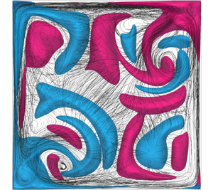
Overview of the transition at  ${Ha}=200$. (a–d) Vertical velocity isosurfaces
 $u_z = \pm 0.1$ (pink/blue) and instantaneous streamlines (black) from the top view. (e) Comparison of data points to linear theory. (a)
 $Ra=5\times 10^{5}$; (b)
 $Ra=1\times 10^{6}$; (c)
 $Ra=2\times 10^{6}$; (d)
 $Ra=5\times 10^{6}$.

At  ${\textit {Ha}}=200$, wall-mode equilibrium solutions are observed at
 ${\textit {Ra}}=4\times 10^5$ to
 ${\textit {Ra}}=6\times 10^5$ (see phase portrait and time series data in figure 5a) with a
 $\mathbb {Z}_4$ symmetry (figure 4a). With increased
 ${\textit {Ra}}$, the wall-mode protrusions extend into the centre of the domain, similarly to the equilibria at
 ${\textit {Ha}}=500$ (§ 3.1). However, by
 ${\textit {Ra}}=1\times 10^6$, a symmetry-breaking bifurcation has occurred, resulting in a state with
 $\mathbb {Z}_2$ symmetry (figure 4b), which produces a periodic solution (figure 5b) with period
 $\mathcal {T}=82.8$ and marks the breakdown of the rolls near the sidewalls which existed between the wall modes. Physically, the wall modes at
 ${\textit {Ra}}=1\times 10^6$ consist of two vortices, one near the corner of the domain and one near the outer tip of the wall mode. The outermost of these is seen to contract and extend away from and into the centre of the domain, periodically switching between being biased to one side of the diagonal and being biased to the other (animated versions of figures 4 and 7 can be found in the supplementary movies available at https://doi.org/10.1017/jfm.2023.863). Of note is that wall modes at
 ${\textit {Ra}}=1\times 10^6$ coexist with a large-scale roll in the centre of the domain, orientated about the diagonal as shown in figure 6. At these values of
 ${\textit {Ra}}$, the orientation of the large-scale roll is seen to oscillate back and forth with the wall modes as they contract and expand. However, as
 ${\textit {Ra}}$ is increased to
 $2\times 10^6$, the large-scale roll begins to dominate the dynamics, maintaining a fixed diagonal orientation and pinning the wall modes into the position shown in figure 4(c). The wall modes, now pinned close to the corners, produce higher-frequency oscillations due to a rapid churning of the wall-mode vortex closest to the wall. The combined effect of these processes is a weakly aperiodic signal, shown in figure 5(c). Upon further increase of
 ${\textit {Ra}}$, the
 $\mathbb {Z}_2$ symmetry is seen to break, and aperiodic solutions are observed at
 ${\textit {Ra}}=5\times 10^6$ and
 ${\textit {Ra}}=1\times 10^7$ (figure 5d). These solutions exhibit chaotic behaviour in the velocity fields and are seen to contain more small-scale structures (figure 4d), which appear to be associated with more chaotic wall mode dynamics that invade the bulk of the domain. Although masked by the small-scale chaotic dynamics in the instantaneous velocity fields, clear evidence of a large-scale roll can still be seen in the mean flow at these higher Rayleigh numbers (see figure 9a for example).
Phase portrait consisting of thermal energy  $E_T$, vertical kinetic energy
 $E_w$ and cross-plane kinetic energy
 $E_u+E_v$, and dimensionless heat transport
 ${\textit {Nu}}$ time series data for each value of
 ${\textit {Ra}}$ considered at
 ${\textit {Ha}}=200$. Here the colours highlight different parts of the
 ${\textit {Nu}}$ time series for easy comparison with the corresponding phase portrait. (a)
 $Ra=5\times 10^{5}$; (b)
 $Ra=1\times 10^{6}$; (c)
 $Ra=2\times 10^{6}$; (d)
 $Ra=5\times 10^{6}$.

Vertical velocity isosurfaces  $u_z = \pm 0.1$ (pink/blue) and instantaneous streamlines (black), showing coexistence of wall modes and large-scale circulation at
 $Ha=200$,
 $Ra=10^6$: (a) top view; (b) three-dimensional view; (c) angled side view.

Overview of the transition at  ${Ha}=1000$. Vertical velocity isosurfaces
 $u_z = \pm 0.01$ (a–e) and
 $u_z = \pm 0.025$ (f–h) (pink/blue), and instantaneous streamlines (black), from the top view. (i) Comparison of data points to linear theory. (a)
 $Ra=5\times 10^{6}$; (b)
 $Ra=7\times 10^{6}$; (c)
 $Ra=8\times 10^{6}$; (d)
 $Ra=9\times 10^{6}$; (e)
 $Ra=1\times 10^{7}$; (f)
 $Ra=1.5\times 10^{7}$; (g)
 $Ra=2\times 10^{7}$; (h)
 $Ra=5\times 10^{7}$.

At  ${\textit {Ha}}=1000$, the wall-mode equilibrium solution appears to have a similar structure to those at lower magnetic field strengths, featuring the same
 $\mathbb {Z}_4$ symmetry, although the characteristic length scale of the wall modes is affected by the magnetic field. The result of this is that the wall-mode protrusions become shorter and thinner compared to the length scale along the sidewall (compare figure 7a to figure 2c, for example). This is consistent with the linear theory, which suggests that the most unstable sidewall mode spatially decays into the bulk with
 ${\textit {Ha}}^{-1/2}$ at leading order, thus producing a thinner sidewall layer at higher
 ${\textit {Ha}}$ (Busse Reference Busse2008). At increased
 ${\textit {Ra}}$, the equilibrium solution undergoes a Hopf bifurcation, resulting in the simple limit cycle oscillation (
 $\mathcal {T}=13.8$) observed at
 ${\textit {Ra}}=7\times 10^6$ (figure 8b), which maintains the
 $\mathbb {Z}_4$ symmetry. This periodic signal arises from an oscillation of the wall-mode protrusions themselves, which synchronously flap back and forth across the diagonal (figure 7b). As
 ${\textit {Ra}}$ is further increased to
 ${\textit {Ra}}=8\times 10^6$, the amplitude of the wall-mode nose oscillations increases as the protrusions extend further into the domain (figure 7c), appearing to violently crash into the sidewall rolls between the wall modes. This modulates the amplitude of the flapping, damping the wall-mode protrusions to a straighter position, closer to the equilibrium solution seen at
 ${\textit {Ra}}=5\times 10^6$. The protrusions then undergo an instability and quickly return to a large-amplitude flapping motion, which damps again, continuing the cycle. Autocorrelation of the
 ${\textit {Nu}}$ time series exhibits decays that scale as
 $\exp ({-\lambda \tau })$ with
 $\lambda \approx 0.041$ for time lag
 $\tau$. The mathematical interpretation of this behaviour is made clearer by the phase portrait and time series data in figure 8(c), where the solution appears to decay along the stable manifold of a saddle point before being ejected along the unstable manifold of the saddle; i.e. the solution appears to shadow an orbit homoclinic to a saddle focus, with the saddle point having a similar flow structure to that of the equilibrium found at
 ${\textit {Ra}}=5\times 10^6$. This behaviour is reminiscent of the Shilnikov phenomenon (Wiggins Reference Wiggins1988), which arises in the third-order system first studied by Shilnikov (Reference Shilnikov1965).
Phase portrait consisting of thermal energy  $E_T$, vertical kinetic energy
 $E_w$ and cross-plane kinetic energy
 $E_u+E_v$, and dimensionless heat transport
 ${\textit {Nu}}$ time series data for each value of
 ${\textit {Ra}}$ considered at
 ${\textit {Ha}}=1000$. Here the colours highlight different parts of the
 ${\textit {Nu}}$ time series for easy comparison with the corresponding phase portrait. (a)
 $Ra=5\times 10^{6}$; (b)
 $Ra=7\times 10^{6}$; (c)
 $Ra=8\times 10^{6}$; (d)
 $Ra=9\times 10^{6}$; (e)
 $Ra=1\times 10^{7}$; (f)
 $Ra=1.5\times 10^{7}$; (g)
 $Ra=2\times 10^{7}$; (h)
 $Ra=5\times 10^{7}$.

By  ${\textit {Ra}}=9\times 10^6$, the ejections are more frequent (figure 8d), with
 ${\textit {Nu}}$ autocorrelations decaying with
 $\lambda \approx 0.078$, and the protrusions exhibit stronger and more complex flapping behaviour, as seen in figure 7(d). At
 ${\textit {Ra}}=1\times 10^7$, the flow is observed undergoing a break in symmetry, resulting in a bursting limit cycle with period
 $\mathcal {T}=147.2$ (figure 8e). The velocity field reveals that three wall-mode structures move across opposing sidewalls, which subsequently collide with the end sidewall, producing a large flap from the end wall mode, as shown in figure 7(e), which then decays to the original flow field. This large flap produces a large increase in the dimensionless heat transport, resulting in the bursting behaviour observed in the Nusselt-number time series data shown in figure 8(e). At
 ${\textit {Ra}}=1.5\times 10^7$, the
 $\mathbb {Z}_4$ symmetry has been fully broken and has been replaced by the
 $\mathbb {Z}_2$ symmetry. This state sustains large periodic wall-mode flapping in two opposing corners, which converges to the limit cycle (
 $\mathcal {T}=31.2$) shown in figure 8(f). Interestingly, this state also features steady convection in the bulk, which occurs at a Rayleigh number higher than
 ${\textit {Ra}}_{c,b}$ (figure 7i), and features a thin roll, aligned along the diagonal, in the centre of the domain (figure 7f). Additionally, as
 ${\textit {Ra}}$ is increased further to
 $2\times 10^7$, this large-scale roll appears in the mean flow field (figure 9b), and the bulk is dominated by vertical flow structures which interact heavily with now chaotically flapping wall-mode protrusions, which extend far into the domain and shed large-scale structures into the bulk as shown at
 ${\textit {Ra}}=2\times 10^7$ in figure 7(g). However, by
 ${\textit {Ra}}=5\times 10^7$, no evidence of such a large-scale roll is observed in the instantaneous or mean flow (figure 9c), unlike in the
 ${\textit {Ha}}=200$ case. Chaotic solutions ensue, with a combination of unsteady bulk dynamics in the form of interconnected columnar structures and the remnants of more chaotic wall-mode dynamics in the corners, similar to the cellular regimes observed previously (Liu et al. Reference Liu, Krasnov and Schumacher2018; Akhmedagaev et al. Reference Akhmedagaev, Zikanov, Krasnov and Schumacher2020; Zürner et al. Reference Zürner, Schindler, Vogt, Eckert and Schumacher2020; Xu et al. Reference Xu, Horn and Aurnou2023). The destruction of the large-scale roll at
 ${\textit {Ha}}=1000$ has occurred by at most
 ${\textit {Ra}}/{\textit {Ra}}_{c,b} \approx 4.84$ (
 ${\textit {Ra}}=5\times 10^7$), whereas at
 ${\textit {Ha}}=200$, the large-scale roll has been seen to persist in our simulations up to at least
 ${\textit {Ra}}/{\textit {Ra}}_{c,b} \approx 218.36$ (
 ${\textit {Ra}}=1\times 10^8$). This shows the clear impact of the magnetic field on the large-scale circulation.
Mean vertical velocity isosurfaces  $u_z = \pm 0.1$ (a) and
 $u_z = \pm 0.05$ (b,c) (pink/blue), and streamlines of mean flow (black), from the angled side view. (a)
 $Ha=200, Ra=10^{7}$; (b)
 $Ha=1000, Ra= 2\times 10^{7}$; (c)
 $Ha=1000, Ra=5\times 10^{7}$.

The transition process near onset at  ${\textit {Ha}}=500$ is seen to be qualitatively more similar to the transition at
 ${\textit {Ha}}=1000$, with a Hopf bifurcation leading to a limit cycle with a
 $\mathbb {Z}_4$ symmetry, which subsequently undergoes a break in symmetry to a
 $\mathbb {Z}_2$ state. However, the highest-
 ${\textit {Ra}}$ simulations (
 ${\textit {Ra}} = 5\times 10^8$) carried out at
 ${\textit {Ha}}=500$ show a large-scale roll in the mean flow, as in the
 ${\textit {Ha}}=200$ case at high supercriticalities, and unlike in the
 ${\textit {Ha}}=1000$ case, where a cellular regime is observed at high
 ${\textit {Ra}}$.
4. Conclusions
We have studied three-dimensional quasistatic magnetoconvection for Hartmann numbers between  $200 \leq {\textit {Ha}} \leq 1000$ in a cube
 $(\varGamma =1)$ with no-slip boundaries, tracking the base state to states exhibiting chaotic multi-scale dynamics. In line with the linear theory in semi-infinite domains, we confirm that the primary instability in this system comes from the sidewalls, giving rise to an equilibrium wall-mode solution for all values of
 ${\textit {Ha}}$ considered. However, the later stages of the transition to chaos past this primary instability are seen to vary with
 ${\textit {Ha}}$. At
 ${\textit {Ha}}=200$, the basic wall-mode state undergoes a symmetry break from a
 $\mathbb {Z}_4$ to a
 $\mathbb {Z}_2$ symmetry, giving rise to limit cycles involving a large-scale roll which re-orientates in time with wall-mode oscillations. At increased Rayleigh numbers, the large-scale roll is seen to persist, accompanied by more chaotic dynamics from the wall modes. However, at
 ${\textit {Ha}}=1000$, the equilibrium wall-mode state undergoes a Hopf bifurcation, resulting in limit cycles involving synchronous oscillations of the wall-mode protrusions, which further evolve to states that shadow an orbit homoclinic to a saddle focus involving more complex oscillatory behaviour. The system then undergoes a
 $\mathbb {Z}_4$-to-
 $\mathbb {Z}_2$ symmetry-breaking bifurcation, producing limit cycles featuring a large-scale roll which is dominated by more vigorous wall-mode oscillations, which subsequently begin to shed large-scale structures into the bulk. At higher
 ${\textit {Ra}}$ this develops to form the cellular regime, and no large-scale roll persists.
The degree to which the results of this study generalise to other geometries, aspect ratios and magnetic boundary conditions is not currently clear. In boxes of larger aspect ratio, it is expected that similar dynamics could occur, and indeed some evidence of potential wall-mode nose flapping can be seen in some flow snapshots in the  $\varGamma =4$ system of Liu et al. (Reference Liu, Krasnov and Schumacher2018), although the short run times of these simulations mean that this cannot be confirmed, and furthermore, it is unclear whether such oscillations are synchronised between the larger number of wall modes. In cylindrical containers there is also some evidence of extended wall-mode protrusions and potential dynamics in the flow snapshots presented by Zürner et al. (Reference Zürner, Schindler, Vogt, Eckert and Schumacher2020) and Xu et al. (Reference Xu, Horn and Aurnou2023), although the continuous symmetry in this geometry appears to result in less strict wall-mode symmetries in some instances, and dynamics such as those described here have not yet been identified. It is currently unclear whether wall modes persist in more generalised geometries. However, wall modes in rotating convection have been seen to persist independently of the geometry in both numerical and experimental studies (Favier & Knobloch Reference Favier and Knobloch2020; Ecke et al. Reference Ecke, Zhang and Shishkina2022). With respect to magnetic boundary conditions, we expect that the results here would generalise to low but finitely conducting boundaries, such as those found in experiments. The reason is that wall modes arise from a suppression of the Lorentz force near the boundary, largely due to electrically insulated boundaries. However, an investigation into the subsequent bifurcations from the basic wall-mode state and dynamics of the ensuing states as discussed here has not yet been carried out experimentally.
Here, we focused on the identification of a large number of flow states, including equilibria, limit cycles and chaotic dynamics, to map out the parameter space and to compare with results from linear stability of wall-mode and bulk onset. Further analysis is currently underway to describe the transition to turbulence, for instance through a series of bifurcations. Preliminary results suggest the presence of multiple states and hysteresis. In the context of pattern formation, the possibility of hysteresis in this system has been suggested in experimental studies (Zürner et al. Reference Zürner, Schindler, Vogt, Eckert and Schumacher2020).
Supplementary movies
Supplementary movies are available at https://doi.org/10.1017/jfm.2023.863.
Acknowledgements
The authors thank G.M. Vasil for fruitful discussions.
Funding
This work was supported by the Deutsche Forschungsgemeinschaft (SPP1881 ‘Turbulent Superstructures’ grants Sh405/7, Sh405/16 and Li3694/1) and used the ARCHER2 UK National Supercomputing Service (https://www.archer2.ac.uk), with resources provided by the UK Turbulence Consortium (EPSRC grants EP/R029326/1 and EP/X035484/1).
Declaration of interests
The authors report no conflict of interest.



