1. Introduction
Turbulent thermal convection is a process occurring widely in nature and technology. Its fundamental mechanisms have been studied for more than a century for the simplified case of a fluid layer heated from below and cooled from above, i.e. Rayleigh–Bénard convection (RBC) (cf. the reviews by Ahlers, Grossmann & Lohse Reference Ahlers, Grossmann and Lohse2009; Lohse & Xia Reference Lohse and Xia2010; Chillà & Schumacher Reference Chillà and Schumacher2012). In classical RBC, smooth heating and cooling plates are considered and in experiments much effort is spent to realise this ideal case, while in most applications roughness or obstacles play an important role. On the one hand, rough surfaces reflect realistic configurations, e.g. convection in the atmosphere is influenced by the roughness of the Earth’s surface. On the other hand, in many industrial applications surface roughness is used in order to increase the heat transport, e.g. in heating/cooling devices. Thus, the consideration of the roughness of the heating and cooling plates in numerical studies has the following advantage: it connects the simplified smooth case with more realistic configurations and, owing to the existing knowledge about the smooth case, allows the separation of the influence of the roughness from the usual mechanisms of turbulent thermal convection.
Most of the studies considering RBC with rough walls so far have been experimental ones: the heat flux and related quantities for a fixed roughness type and varying Rayleigh number
 $\mathit{Ra}$
are usually measured. This is mainly due to the fact that changing the roughness configuration requires expensive constructions of multiple heating and cooling plates. There have been different results with respect to the scaling of the integral heat flux, i.e. the Nusselt number
 $\mathit{Nu}$
, as a power law
 $\mathit{Nu}={\it\alpha}\,\mathit{Ra}^{{\it\beta}}$
in these experimental studies. In the experiments by Shen, Xia & Tong (Reference Shen, Xia and Tong1996) an increase of the pre-factor
 ${\it\alpha}$
of approximately 20 % was reported, occurring only if the height of the obstacles is larger than the mean thickness of the thermal boundary layer (BL)
 ${\it\delta}_{T}$
. In another study, Du & Tong (Reference Du and Tong2000) found a stronger increase if the height of the obstacles is increased. A somewhat different result was obtained in the experiments by Roche et al. (Reference Roche, Castaing, Chabaud and Herbal2001), who found an increase of the exponent
 ${\it\beta}$
. Since the resulting
 ${\it\beta}$
was approximately
 $1/2$
, this was interpreted as a triggering of the ultimate regime proposed by Kraichnan (Reference Kraichnan1962), at
 $\mathit{Ra}$
far below that found and explained for the case of smooth plates (Grossmann & Lohse Reference Grossmann and Lohse2011; He et al.
Reference He, Funfschilling, Nobach, Bodenschatz and Ahlers2012). Recent experiments performed by Tisserand et al. (Reference Tisserand, Creyssels, Gasteuil, Pabiou, Gibert, Castaing and Chillà2011) in a cell with smooth cooling and rough heating plates corroborate this increase of
 ${\it\beta}$
to approximately
 $1/2$
, but their analysis showed that it is not caused by increased turbulence, i.e. the final regime. A much weaker increase of
 ${\it\beta}$
was reported by Qiu, Xia & Tong (Reference Qiu, Xia and Tong2005). Ciliberto & Laroche (Reference Ciliberto and Laroche1999) found a difference between a periodic roughness and a power-law distributed one. Only in the case of the power-law distributed roughness was an increase in the exponent
 ${\it\beta}$
obtained.
This result was supported by Villermaux (Reference Villermaux1998), who developed a model explaining the heat flux enhancement in the case of a wide spectrum of typical roughness length scales. It is based on the assumption that the heat flux is proportional to the total covering area of the surface and describes an increase of the scaling exponent
 ${\it\beta}$
of up to 10 % depending on the surface’s fractal dimension. When the roughness is introduced uniformly by obstacles of the same height, the model predicts that
 ${\it\beta}$
remains unchanged.
In numerical simulations (Stringano, Pascazio & Verzicco Reference Stringano, Pascazio and Verzicco2006) found, similarly to some of the experimental results, a weak increase of the scaling exponent
 ${\it\beta}$
.
The differences in the results obtained in particular experiments are usually explained by different types of roughness. Here one distinguishes the roughness introduced by a set of roughness elements of different sizes from that introduced by single-sized elements. In the latter case, the uniform distribution of the elements leads to the so-called regular roughness. Another important issue is whether the roughness height is smaller or larger than the typical BL thickness. Even in the case of a high regular roughness, the experimental results might differ, and this is usually explained by the different shapes of the roughness elements. Thus, Ciliberto & Laroche (Reference Ciliberto and Laroche1999) used spheres, Shen et al. (Reference Shen, Xia and Tong1996) pyramids with square cross-sections, and Roche et al. (Reference Roche, Castaing, Chabaud and Herbal2001) V-shaped grooves. Connected to this is the result by Du & Tong (Reference Du and Tong2000) and Stringano et al. (Reference Stringano, Pascazio and Verzicco2006), stating that the edges of the roughness elements are the most active places of plume emission. All these facts lead to the conclusion that the effect of a rough surface on the heat transport cannot be fully explained by a single geometrical characteristic of the roughness, such as the covering area of the rough surface.
A first step in developing a model that takes the geometrical characteristics of the roughness elements into account has been made by Shishkina & Wagner (Reference Shishkina and Wagner2011) for the case of relatively high and regularly distributed roughness elements. The model decomposes the heat flux from the rough surface into several contributions from separate parts of the roughness elements. These contributions are estimated by applying the Prandtl–Blasius–Pohlhausen theory of laminar BLs. This model is in good agreement with two-dimensional direct numerical simulations (DNS) in which the roughness is realised by rectangular obstacles. Since on the one hand discrepancies between two-dimensional (2D) and three-dimensional (3D) RBC are present in particular for small Prandtl numbers
 $\mathit{Pr}$
(Schmalzl, Breuer & Hansen Reference Schmalzl, Breuer and Hansen2004), and on the other hand deviations of the theory of laminar BLs and DNS results have been obtained (e.g. Wagner, Shishkina & Wagner Reference Wagner, Shishkina and Wagner2012), the comparison of the model with 3D DNS and further model advancement are required. Furthermore, as mentioned earlier, parametric studies of different roughness configurations are difficult to do in experiments, but are required, e.g. during the design process of heat exchangers, where the parameter ranges of
 $\mathit{Ra}$
and
 $\mathit{Pr}$
are fixed while the roughness is optimised.
In the present paper we report on DNS results obtained in a rectangular domain with equal width and height and a depth equal to one-fourth of the height for
 $\mathit{Pr}=0.786$
and
 $\mathit{Ra}$
between
 $10^{6}$
and
 $10^{8}$
. The DNS results for this special geometry with smooth plates (also for other depth/height aspect ratios and in comparison with a cylindrical geometry) have been published earlier (Wagner & Shishkina Reference Wagner and Shishkina2013). Note that this type of domain was previously used in many recent experimental (Xia, Sun & Zhou Reference Xia, Sun and Zhou2003; Vasil’ev & Frick Reference Vasil’ev and Frick2011; Zhou & Xia Reference Zhou and Xia2013) and numerical (Huang et al.
Reference Huang, Kaczorowski, Ni and Xia2013; Wagner & Shishkina Reference Wagner and Shishkina2013) studies. Also, the influence of surface roughness has been investigated in such a domain experimentally (Salort et al.
Reference Salort, Liot, Rusaouen, Seychelles, Tisserand, Creyssels, Castaing and Chillà2014). It has the advantage that the global flow structure is pseudo-two-dimensional if
 $\mathit{Ra}$
is sufficiently large (Wagner & Shishkina Reference Wagner and Shishkina2013), while the domain and the physics of the (turbulent) flow is three-dimensional. This simplifies the analysis and allows planar measurements.
The surface roughness in the present DNS is realised by attaching four box-shaped obstacles to the heating as well as the cooling plate. Besides varying
 $\mathit{Ra}$
, the height and width of the obstacles are also varied. It should be noted that in the context of RBC the term roughness is usually used even if the roughness elements are larger than the thicknesses of the viscous and thermal BLs. This is contrary to other literature on the influence of roughness (e.g. Jiménez Reference Jiménez2004), in which the term roughness is only used if the roughness elements are hidden within the BLs; otherwise the roughness elements are called obstacles or grooves (see also the discussion by Stringano et al.
Reference Stringano, Pascazio and Verzicco2006). In the present paper we use the word roughness to highlight the similarities to experimental RBC studies. Nevertheless, when talking about the single roughness elements and their characteristics, we use the word obstacles.
In § 2 the numerical method and the general set-up are described. The numerical results on the heat transport enhancement are given in § 3. By considering and matching two limiting cases, a simple model for the heat flux enhancement without any free parameter is constructed in § 4. Furthermore, the numerical results on the global flow structure as well as the velocity distributions in the convection cells with rough heated and cooled plates are discussed in § 5. In § 6 the numerical results are set in relation to theoretical and experimental results from the literature. Finally, the paper is closed by presenting some conclusions in § 7.
2. Numerical methodology and set-up
A fourth-order-accurate finite-volume code working in Cartesian coordinates (Shishkina, Shishkin & Wagner Reference Shishkina, Shishkin and Wagner2009) has been used to solve the dimensionless equations describing the conservation of mass, momentum and energy in the Oberbeck–Boussinesq approximation, i.e.
 $$\begin{eqnarray}\displaystyle & \displaystyle \frac{\partial \boldsymbol{u}}{\partial t}+(\boldsymbol{u}\boldsymbol{\cdot }\boldsymbol{{\rm\nabla}})\boldsymbol{u}=-\boldsymbol{{\rm\nabla}}p+\sqrt{\frac{\mathit{ Pr }}{\mathit{Ra}}}\,{\rm\nabla}^{2}\boldsymbol{u}+T\boldsymbol{e}_{z}, & \displaystyle\end{eqnarray}$$
 $$\begin{eqnarray}\displaystyle & \displaystyle \frac{\partial T}{\partial t}+(\boldsymbol{u}\boldsymbol{\cdot }\boldsymbol{{\rm\nabla}})T=\sqrt{\frac{1}{\mathit{Pr}\,\mathit{Ra}}}\,{\rm\nabla}^{2}T,\quad \boldsymbol{{\rm\nabla}}\boldsymbol{\cdot }\boldsymbol{u}=0. & \displaystyle\end{eqnarray}$$
 $\boldsymbol{u}$
denotes the velocity,
 $t$
time,
 $p$
pressure,
 $T$
temperature and
 $\boldsymbol{e}_{z}$
the unit vector in the vertical direction. For non-dimensionalisation, the free-fall velocity
 $\sqrt{\widehat{{\it\alpha}}\,\widehat{g}\widehat{{\rm\Delta}}\widehat{H}}$
and the height
 $\widehat{H}$
have been used. Further, the temperature is non-dimensionlised as
 $T=(\widehat{T}-\widehat{T}_{M})/\widehat{{\it\Delta}}$
, where dimensional quantities are marked with a hat and
 $\widehat{T}_{M}=(\widehat{T}_{bottom}+\widehat{T}_{top})/2$
and
 $\widehat{{\it\Delta}}=\widehat{T}_{bottom}-\widehat{T}_{top}$
. As usual for the Oberbeck–Boussinesq approximation, the kinematic viscosity
 $\widehat{{\it\nu}}$
, the thermal diffusivity
 $\widehat{{\it\kappa}}$
, the thermal expansion coefficient
 $\widehat{{\it\alpha}}$
, the gravitational acceleration
 $\widehat{g}$
and the density
 $\widehat{{\it\rho}}$
are assumed to be constant. To allow buoyant motion, a linear temperature dependence of the density only in the buoyancy term is assumed. Under these conditions, the dynamics of the flow is governed by the Rayleigh number
 $\mathit{Ra}=\widehat{{\it\alpha}}\,\widehat{g}\widehat{{\rm\Delta}}\widehat{H}^{3}/(\widehat{{\it\nu}}\,\widehat{{\it\kappa}})$
and the Prandtl number
 $\mathit{Pr}=\widehat{{\it\nu}}/\widehat{{\it\kappa}}$
. The latter we fix to
 $\mathit{Pr}=0.786$
in all our simulations.
The domain height
 $H$
and width
 $L$
are chosen equal, while the depth
 $D$
is one-fourth of the height. The top and bottom plates are isothermal with
 $T_{bottom}>T_{top}$
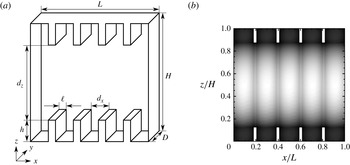
, the vertical sidewalls are adiabatic and on all surfaces the velocity vanishes due to the no-slip condition. To simulate the influence of the surface roughness of the top and bottom plates, four obstacles with height
 $h$
and width
 $\ell$
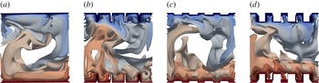
are placed equidistantly on each of these plates (see also the sketch in figure 1(a) and the visualisation of the flow in figure 2). These obstacles have temperatures
 $T_{top},T_{bottom}$
, respectively, as do the surfaces they are attached to.
(a) Sketch of the domain with coordinate system and nomenclature. (b) Distribution of mesh spacing
 $\sqrt{{\it\Delta}_{x}{\it\Delta}_{z}}$
(black small, white large) in the
 $x{-}z$
-plane (at arbitrary
 $y$
) for a certain shape of obstacles, where
 ${\it\Delta}_{x}$
,
 ${\it\Delta}_{z}$
are the mesh spacings in the
 $x$
-,
 $z$
-direction, respectively.

Instantaneous temperature isosurfaces (red
 $=$
warm, blue
 $=$
cold) for smooth plates (a) and plates with obstacles of size (b)
 $h=0.125H,\ell =0.025L$
, (c)
 $h=0.025H$
,
 $\ell =0.125L$
and (d)
 $h=0.125H,\ell =0.125L$
for
 $\mathit{Ra}=10^{7},\mathit{Pr}=0.786$
.

To allow effective DNS in such a complicated domain, the capacitance matrix technique has been used for a non-iterative calculation of the pressure field. To further decrease the computational effort, the extent of the obstacles in the
 $y$
-direction is restricted to be equal to the domain depth
 $D$
. Thus the non-equidistant mesh spacing in the
 $x$
- and
 $z$
-directions is independent of
 $y$
, i.e. the
 $y$
-direction is regular. This method has been applied previously to the investigation of mixed (Bailon-Cuba et al.
Reference Bailon-Cuba, Shishkina, Wagner and Schumacher2012; Shishkina & Wagner Reference Shishkina and Wagner2012) and forced (Koerner et al.
Reference Koerner, Shishkina, Wagner and Thess2013) convection in complicated domains.
The spatial resolution has been chosen according to Shishkina et al. (Reference Shishkina, Stevens, Grossmann and Lohse2010). By considering the BL structure analysis by Wagner et al. (Reference Wagner, Shishkina and Wagner2012) and the improved BL structure model by Shishkina, Horn & Wagner (Reference Shishkina, Horn and Wagner2013) and Shishkina, Wagner & Horn (Reference Shishkina, Wagner and Horn2014), the BL resolution has been further refined. Between the obstacles, the mesh has been chosen fine enough also to resolve any flow separation that might occur at the edges of the obstacles. In figure 1(b) the mesh in the
 $x{-}z$
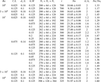
-plane is visualised for a single roughness configuration. This and further different roughness configurations and the corresponding numbers of computational nodes are given in table 1.
Simulation parameters in addition to
 $\mathit{Pr}=0.786$
: the Rayleigh number
 $\mathit{Ra}$
, the width of the obstacles (
 $\ell$
), height (
 $h$
) and distance (
 $d_{x}$
) between the roughness elements, the number of computational nodes
 $N_{i}$
in the
 $i$
-direction (
 $i=x,y,z$
), the number of time units
 ${\it\tau}$
used for averaging, the Nusselt number
 $\mathit{Nu}$
with estimated uncertainty, and the relative increase of the plates covering area (
 $A/A_{s}$
) and of the Nusselt number (
 $\mathit{Nu}/\mathit{Nu}_{s}$
) in comparison with the smooth case.

3. Heat flux enhancement by regular surface roughness
The effect of the roughness on the global heat flux is discussed in two ways. First, the influence of different roughness configurations is compared at constant
 $\mathit{Ra}=10^{7}$
. A previous numerical study in 2D revealed that the heat flux enhancement by roughness cannot be parameterised only by the covering area, the volume of the obstacles, or similar quantities (Shishkina & Wagner Reference Shishkina and Wagner2011). Rather, it depends on more complicated combinations of the height of the obstacles
 $h$
, the width
 $\ell$
, and
 $\mathit{Ra}$
. In the present study we thus vary
 $h$
and
 $\ell$
independently and similarly to the 2D study (see table 1 for details). Second, for two different roughness configurations (slender and wide obstacles of the same height) the Rayleigh number is varied. Thereby not only the global heat flux but also contributions from different parts of the obstacles are studied.
3.1. Heat flux for different roughness configurations
As usual in RBC, we consider the heat flux
 $\boldsymbol{q}$
by convection and conduction in relation to the heat flux for a fluid at rest. In our units, this is
 $\boldsymbol{q}=\sqrt{\mathit{Ra }\,\mathit{Pr}}\,\boldsymbol{u}T-\boldsymbol{{\rm\nabla}}T$
. From (2.2) one can derive that for adiabatic vertical sidewalls, the Nusselt number
 $\mathit{Nu}(z)=\langle \boldsymbol{q}\boldsymbol{\cdot }\boldsymbol{e}_{z}\rangle _{t,A_{s}}$
is independent of the vertical position
 $z$
for
 $h\leqslant z\leqslant H-h$
and infinite averaging time. Here,
 $\langle \,f\rangle _{t,A_{s}}$
denotes the average of the quantity
 $f$
over time and the horizontal cross-section
 $A_{s}$
of the domain, i.e. the covering area of the smooth bottom plate. Furthermore, the integral heat flux
 $Q=A\langle \boldsymbol{q}\boldsymbol{\cdot }\boldsymbol{n}\rangle _{t,A}$
entering/leaving the fluid through the bottom/top plates, respectively, must be equal to
 $\mathit{Nu}\,A_{s}$
. Here
 $\boldsymbol{n}$
is the (local) normal vector of the rough surface and
 $A=D(L+8h)$
is its covering area. Thus in the following we will only discuss
 $\mathit{Nu}=Q/A_{s}$
and compare it with the Nusselt number of the smooth case
 $\mathit{Nu}_{s}$
.
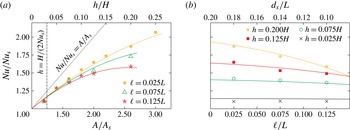
In figure 3(a), the heat flux ratio
 $\mathit{Nu}/\mathit{Nu}_{s}$
is plotted against the relative covering area
 $A/A_{s}$
. This means that the height of the obstacles
 $h$
is varied for particular values of the width
 $\ell$
. (See also the additional abscissa for the corresponding obstacle height at the top of the plot.) We observe that the
 $\mathit{Nu}$
-scaling never reaches the line
 $\mathit{Nu}/\mathit{Nu}_{s}=A/A_{s}$
(the black dotted line in figure 3
a), which would indicate that
 $Nu/Nu_{s}$
is directly proportional to
 $A/A_{s}$
. Furthermore, the larger
 $h$
and
 $\ell$
get, the stronger is the deviation from this line. Although Du & Tong (Reference Du and Tong2000) obtained in their experiments for
 $A/A_{s}=1.41$
a relative increase of the heat flux of
 $\mathit{Nu}/\mathit{Nu}_{s}=1.76$
, we never observed the case
 $\mathit{Nu}\geqslant \mathit{Nu}_{s}(A/A_{s})$
. The experiments by Du & Tong (Reference Du and Tong2000) were conducted in a cylindrical container filled with water for
 $5\times 10^{8}\lesssim \mathit{Ra}\lesssim 10^{11}$
and with V-shaped grooves in the heating and cooling plates.
Influence of the obstacle configuration on the relative increase of the Nusselt number compared to the smooth case,
 $\mathit{Nu}/\mathit{Nu}_{s}$
, as obtained in the DNS for
 $\mathit{Ra}=10^{7}$
and
 $\mathit{Pr}=0.786$
(symbols). The same numerical data are presented in two different ways. (a) The height of the obstacles
 $h$
is varied for different obstacle widths
 $\ell$
, which corresponds to an increase of the plate covering area
 $A$
compared to that in the smooth case,
 $A_{s}$
. The empirical functions (3.2) for different
 $\ell$
are shown as solid lines. (b) For different obstacle heights, the width of the obstacles is varied, which can be also understood as a varying distance
 $d_{x}$
between the obstacles. Solid lines represent the empirical relation (3.2) for different
 $h$
.

The main focus of the present paper is on the influence of regularly distributed obstacles with a height
 $h$
larger than the mean thickness of the thermal BL, which can be defined for the smooth case as
 ${\it\delta}_{T,s}\equiv H/(2\,\mathit{Nu}_{s})$
. Since for
 $\mathit{Ra}=10^{7}$
we find
 $\mathit{Nu}_{s}=16.4$
(Wagner & Shishkina Reference Wagner and Shishkina2013) and thus
 ${\it\delta}_{T,s}\approx 0.03H$
, apart from
 $h=0.025H$
the tips of the obstacles are not hidden in the thermal BL. For clarity we have marked
 ${\it\delta}_{T,s}$
in figure 3(a) by a vertical black dashed line.
Similarly to Shishkina & Wagner (Reference Shishkina and Wagner2011) we conclude that the covering area
 $A$
is not a universal characteristic for describing the heat flux increase; otherwise all the graphs in figure 3(a) would collapse. Further, figure 3(a) reveals that for small
 $A/A_{s}$
the Nusselt number increases almost linearly with the covering area. For
 $A$
larger than a critical value
 $A_{crit}$
(or
 $h$
larger than a certain critical height), deviations from this linear dependence become apparent. Thereby
 $A_{crit}$
seems to decrease with increasing
 $\ell$
, therefore for large
 $A$
the graphs for different
 $\ell$
do not collapse. For a fixed covering area and fixed number of obstacles, the largest heat flux enhancement is obtained for small
 $\ell$
, i.e. a large distance
 $d_{x}$
between the obstacles. This result is also supported by figure 3(b), in which for particular values of
 $h$
the relative heat flux increase is plotted against the width of the obstacles
 $\ell$
. We observe that, especially for large
 $h$
, the heat flux decreases with increasing
 $\ell$
, while the covering area of the surface remains constant. To achieve a large heat flux, it is thus not sufficient to have a large covering area: there must also be enough space
 $d_{x}$
between the obstacles. For a fixed covering area and increasing obstacle height, larger
 $d_{x}$
is required to obtain the maximum heat flux.
Based on the analysis of the DNS data presented in figure 3, we create an approximation of the relative heat flux deviation due to the regular surface roughness.
As one can see in figure 3(a), at least for small obstacle height
 $h$
, the relative heat flux increases proportionally to
 $h$
and almost independently of the obstacle width
 $\ell$
. With further increase in the obstacle height, a certain dependence on the obstacle width
 $\ell$
becomes apparent. Therefore, we seek an approximation of the form
 $$\begin{eqnarray}\mathit{Nu}/\mathit{Nu}_{s}=1+c_{1}(h/H)+c_{2}(h/H)^{2}f(\ell /L),\end{eqnarray}$$
where
 $c_{1}$
and
 $c_{2}$
are constants and the function
 $f$
depends only on the obstacle width
 $\ell$
. It turns out that the function
 $f$
can be well approximated by an exponential function.
The constants
 $c_{1},c_{2}$
and the details of the function
 $f$
are determined by fitting the DNS data, which leads to the following empirical function describing the heat flux increase by roughness in the parameter range considered:
 $$\begin{eqnarray}\displaystyle \mathit{Nu}/\mathit{Nu}_{s} & {\approx} & \displaystyle 1+5.84\,(h/H)-5.87\,\exp (7.42\,\ell /L)(h/H)^{2}\nonumber\\ \displaystyle & = & \displaystyle 1+0.73r-0.0917\,\exp (7.42\,\ell /L)r^{2}.\end{eqnarray}$$
Here the heat flux increase can be also expressed as a function of the relative increase of the surface area due to the roughness
 $r\equiv (A-A_{s})/A_{s}$
. Equation (3.2) is evaluated for the
 $\ell$
values considered and plotted in figure 3(a,b) with solid lines. Note that the approximation obtained has an unphysical global maximum outside the
 $h$
-range considered. This could be circumvented by a more sophisticated ansatz also valid for even larger
 $h$
.
Even though the interpretation of the physics behind this empirical relation seems rather difficult, it is able to represent the main findings in the numerical data. Thus, the heat flux increase due to the obstacles can be connected (for fixed Rayleigh number) to purely geometric properties of the obstacles.
A heat flux increase due to roughness, which is smaller than
 $\mathit{Nu}/\mathit{Nu}_{s}=A/A_{s}$
, can be understood as an increased mean thickness of the thermal BL
 ${\it\delta}_{T}$
in the rough case compared to the smooth case. For the latter we defined above
 ${\it\delta}_{T,s}\equiv H/(2\,\mathit{Nu}_{s})$
. To get a consistent definition for the rough cases
 ${\it\delta}_{T,rough}$
, we have to keep in mind that we used the horizontal cross-section of the domain
 $A_{s}=DL$
for the definition of
 $\mathit{Nu}$
and not the actual covering area
 $A$
of the rough surface. Thus, we define
 $$\begin{eqnarray}{\it\delta}_{T,rough}\equiv (H/(2\,\mathit{Nu}))(A/A_{s}),\end{eqnarray}$$
so that only for
 $\mathit{Nu}/\mathit{Nu}_{s}=A/A_{s}$
is the mean thicknesses of the thermal BL in the rough and smooth cases equal. Since we find for all roughness configurations that
 $\mathit{Nu}/\mathit{Nu}_{s}<A/A_{s}$
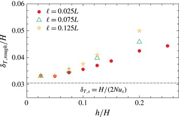
, we can deduce that roughness influences the increase of the mean thickness of the thermal BL. Thus,
 ${\it\delta}_{T,rough}$
increases for both increasing obstacle height
 $h$
and width
 $\ell$
, as shown in figure 4.
Comparison of the mean thickness of the thermal BL,
 ${\it\delta}_{T,rough}$
, (cf. (3.3)) for different roughness configurations and
 $\mathit{Ra}=10^{7}$
.

To understand the processes leading to the above results in more detail, we decompose the total heat flux entering the container through the heated rough bottom plate
 $Q=A\langle \boldsymbol{q}\boldsymbol{\cdot }\boldsymbol{n}\rangle _{t,A}$
into three contributions
 $Q_{i}$
:
 $$\begin{eqnarray}Q=\mathop{\sum }_{i}Q_{i}=Q_{bottom}+Q_{top}+Q_{side}.\end{eqnarray}$$
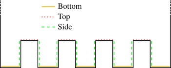
The three contributions correspond to different parts of the rough surface as sketched in figure 5.
Two-dimensional sketch and nomenclature for the different contributions to the total heat flux
 $\mathit{Nu}$
entering the fluid at the rough bottom plate.

 $Q_{bottom}$
is the heat flux entering the fluid through the horizontal surfaces between the obstacles, while
 $Q_{top}$
is the contribution from the horizontal surfaces and
 $Q_{side}$
from the vertical surfaces of the obstacles. From these three contributions, we calculate the local Nusselt numbers, defined as
 $$\begin{eqnarray}\mathit{Nu}_{i}\equiv \frac{Q_{i}}{A_{i}}\quad \text{with}~A_{i}\equiv \left\{\begin{array}{@{}ll@{}}4\,\ell D\quad & \text{for}~i=\text{top},\\ 5\,d_{x}D\quad & \text{for}~i=\text{bottom},\\ 8\,hD\quad & \text{for}~i=\text{side}.\end{array}\right.\end{eqnarray}$$
These
 $\mathit{Nu}_{i}$
can be used to define the thermal BL local thickness
 ${\it\delta}_{T,i}\equiv H/(2\,\mathit{Nu}_{i})$
. In addition we define the local Nusselt number for the horizontal parts of the obstacles (top, bottom)
 $\mathit{Nu}_{horizontal}=(Q_{bottom}+Q_{top})/(DL)$
.
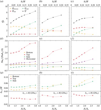
(a–c) The different contributions
 $Q_{i}$
to the global heat flux
 $Q$
from the top and side surfaces of the obstacles and from the bottom surface between the obstacles. (d–f) Local Nusselt number
 $\mathit{Nu}_{i}$
for different parts
 $i$
of the roughness elements as defined in (3.5) in units of the globally averaged heat flux as expressed by
 $\mathit{Nu}\,A_{s}/A$
. (g–i) The mean thickness of the thermal BL,
 ${\it\delta}_{T,i}$
, at different positions of the rough surface, as defined in the text. For comparison,
 ${\it\delta}_{T,s}$
for the smooth case is given as a horizontal solid black line. Besides the surface area
 $A$
(or the height of the obstacles), the obstacle width
 $\ell$
is also varied: (a,d,g)
 $\ell =0.025L$
, (b,e,h)
 $\ell =0.075L$
and (c, f,i)
 $\ell =0.125L$
.
 $\mathit{Ra}=10^{7},\mathit{Pr}=0.786$
.

Since the
 $Q_{i}$
are expected to depend on the size of the corresponding surface parts, we discuss additionally the
 $\mathit{Nu}_{i}$
normalised by the globally averaged heat flux
 $Q/A=\mathit{Nu}\,A_{s}/A$
. Furthermore, the local thickness of the thermal BL
 ${\it\delta}_{T,i}$
is compared with the smooth case
 ${\it\delta}_{T,s}$
.
All the different quantities are plotted in figure 6 against the relative increase of the covering area
 $A/A_{s}$
, for different heights
 $h$
and widths
 $\ell$
of the obstacles.
We observe that the global heat flux increase over the smooth case is mainly determined by
 $Q_{side}$
, which for small
 $h$
increases almost linearly with
 $A/A_{s}$
. Similarly to the case of
 $\mathit{Nu}$
in figure 3(a), deviations from the linear trend are more pronounced for larger
 $h$
and
 $\ell$
(cf. figure 6
b,c). These deviations are accompanied by a decrease in
 $Q_{bottom}$
with growing
 $\ell$
, while
 $Q_{bottom}$
is almost independent of
 $h$
. This can be understood as an effect of the stagnation of warm fluid in the cavities between the heated obstacles. (For the sake of simplicity, we discuss only the heating plate, since the cooling plate leads, by symmetry, to equivalent results.) This warm fluid covers the horizontal surfaces between the obstacles and the lower part of the vertical surfaces of the obstacles. Roughly speaking, figure 6 reveals that as soon as
 $d_{x}$
is smaller than the obstacle height,
 $Q_{bottom}$
starts to decrease.
To understand better the contribution of different obstacle surfaces, we additionally consider the mean heat flux from the distinct parts of the obstacles
 $\mathit{Nu}_{i}$
and relate it to the global mean value of the heat flux, i.e.
 $Q/A=\mathit{Nu}\,A_{s}/A$
. The results are shown in figure 6(d–f). We observe that the heat flux entering the fluid from the top surfaces of the obstacles is much larger than the mean value and even increases with
 $h$
. This can be explained by the fact that the obstacle tips are surrounded by colder fluid the deeper they point into the bulk region of the domain. Furthermore the contribution of the obstacle sidewalls is almost unaffected by the height of the obstacles and their width. This means, that their contribution grows purely due to an increased surface area
 $A_{side}$
for increasing
 $h$
. Finally, the contribution from the bottom of the cavities, which is found to be almost equal to the mean value and unaffected by
 $h$
for slender obstacles, is decreased to almost one half of the mean value for wide and high obstacles. Their contribution thus decreases significantly with growing
 $\ell$
as the mean value is decreased and, further, the corresponding surface area is smaller for larger
 $\ell$
.
The differences in the
 $\mathit{Nu}_{i}$
can, by definition, also be understood as differences in the thickness of the thermal boundary at different parts of the rough surface
 ${\it\delta}_{T,i}$
.
The BL thicknesses
 ${\it\delta}_{T,bottom}$
and
 ${\it\delta}_{T,side}$
are larger than those in the case of a smooth heating plate (
 ${\it\delta}_{T,s}$
). Only on top of the obstacles is a much smaller thickness
 ${\it\delta}_{T,top}$
of the thermal BL observed. Since the BL thickness increases along a flat plate (Wagner et al.
Reference Wagner, Shishkina and Wagner2012), it is especially small for slender obstacles (figure 6
d). This result is in good agreement with the experimental result by Salort et al. (Reference Salort, Liot, Rusaouen, Seychelles, Tisserand, Creyssels, Castaing and Chillà2014), who also obtained a decreased BL thickness on top of the roughness elements as is discussed more in § 6. For a fixed
 $\ell$
and increasing
 $h$
, it slightly decreases until a certain threshold is reached, above which
 ${\it\delta}_{T,top}$
remains almost constant. This threshold is reached when the height of the obstacles and the horizontal distance between them are approximately equal.
From this we can deduce that the increase of the mean thickness of the thermal BL
 ${\it\delta}_{T,rough}$
(cf. figure 4) is mainly caused by the stagnating hot fluid between the obstacles.
Thus we describe the heat flux increase due to roughness (cf. (3.2)) in two steps. First, the contribution from the vertical walls of the obstacles leads to an almost linear and
 $\ell$
-independent increase with the obstacle height
 $h$
. Second, for large
 $h$
, an
 $\ell$
-dependent deviation from this trend takes place, which becomes stronger for larger
 $\ell$
, i.e. a smaller distance
 $d_{x}$
between the obstacles. This leads to differences between the heat flux from rough surfaces with equal covering areas as already shown in figure 3.
As a consequence, the largest heat flux increase for a fixed number of obstacles and fixed covering area can be achieved for very slender obstacles, i.e. a large distance
 $d_{x}$
between them. In this case, the heat flux, in comparison with a smooth plate, increases almost linearly with
 $h$
even for very large
 $h$
and thus the optimal heat flux for a given covering area can be reached.
3.2. The influence of roughness on the
 $\mathit{Ra}$
-dependence of the heat flux

Besides the influence of different roughness configurations, we want to compare our results with those from the literature regarding changes in the
 $\mathit{Ra}$
dependence of
 $\mathit{Nu}$
due to surface roughness. For this comparison, we chose two roughness configurations: rather high and slender obstacles (
 $h=0.125H$
,
 $\ell =0.025L$
), and wider obstacles with the same height (
 $h=0.125H$
,
 $\ell =0.125L$
). For both configurations, the covering area of the rough plates is twice that of the smooth plates. In § 3.1 we have already obtained for
 $\mathit{Ra}=10^{7}$
an increase in
 $\mathit{Nu}$
of approximately 65 % for the slender obstacles and only approximately 49 % for the wider ones. We vary
 $\mathit{Ra}$
between
 $10^{6}$
and
 $10^{8}$
and expect the thickness of the thermal BL
 ${\it\delta}_{T,s}\equiv H/(2\,\mathit{Nu}_{s})$
to be between
 $0.015H~(\mathit{Ra}=10^{8})$
and
 $0.065H~(\mathit{Ra}=10^{6})$
. Thus for all
 $\mathit{Ra}$
considered, the roughness height
 $h$
is at least twice as large as
 ${\it\delta}_{T,s}$
. Since in the literature a transition from a smooth
 $\mathit{Nu}$
versus
 $\mathit{Ra}$
scaling to a rough one for obstacle heights
 $h$
of the order of the thickness of the thermal BL
 ${\it\delta}_{T,s}$
has been reported, we do not expect to find such a transition in the scalings of our numerical results due to the larger heights
 $h$
considered in our DNS.
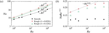
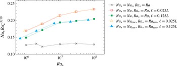
In figure 7(a) we compare the
 $\mathit{Ra}$
-dependences of the smooth (Wagner & Shishkina Reference Wagner and Shishkina2013) and two rough cases. A linear fitting reveals, for the smooth case, an average scaling
 $\mathit{Nu}_{s}=0.116\times \mathit{Ra}^{0.307}$
, while for the slender obstacles we obtain
 $\mathit{Nu}=0.065\times \mathit{Ra}^{0.371}$
and for the wider ones
 $\mathit{Nu}=0.061\times \mathit{Ra}^{0.368}$
. Thus both roughness configurations lead to slightly increased scaling exponents, which is in good agreement with the numerical study by Stringano et al. (Reference Stringano, Pascazio and Verzicco2006), measurements by Qiu et al. (Reference Qiu, Xia and Tong2005) and the two-dimensional numerical investigation by Shishkina & Wagner (Reference Shishkina and Wagner2011). Contrary to the experimental studies by Roche et al. (Reference Roche, Castaing, Chabaud and Herbal2001) and Tisserand et al. (Reference Tisserand, Creyssels, Gasteuil, Pabiou, Gibert, Castaing and Chillà2011), the scaling exponent is not increased to 0.5. This result is interesting, since Tisserand et al. (Reference Tisserand, Creyssels, Gasteuil, Pabiou, Gibert, Castaing and Chillà2011) used rectangular roughness elements, i.e. rather similar to ours, while Stringano et al. (Reference Stringano, Pascazio and Verzicco2006) considered V-shaped grooves and Qiu et al. (Reference Qiu, Xia and Tong2005) used square-based pyramids. In all these cases a cylindrical domain and larger
 $\mathit{Ra}$
were investigated. Thus we conclude that similar results can be obtained even though the roughness configurations are very different. Further, not only the roughness configuration but also
 $\mathit{Ra}$
and
 $\mathit{Pr}$
determine the changes of the heat flux due to roughness. Understanding the
 $\mathit{Pr}$
-dependence goes beyond the scope of the present paper; here we focus only on the
 $\mathit{Ra}$
-dependence.
(a) Comparison of
 $\mathit{Ra}$
-scaling of
 $\mathit{Nu}$
for the smooth case and rough cases with obstacle widths
 $\ell =0.025L$
and
 $\ell =0.125L$
for obstacle height
 $h=0.125H$
and (b)
 $\mathit{Nu}$
reduced by
 $\mathit{Ra}^{0.3}$
for a more detailed view. The lines represent linear fits.

The resulting scaling exponent obtained in our DNS is very similar for both roughness configurations. To get a more detailed view of this, we consider in figure 7(b)
 $\mathit{Nu}$
reduced by the scaling in the smooth case, i.e.
 $\mathit{Ra}^{0.3}$
. Here it becomes obvious that the power-law fits reflect only an average scaling for the
 $\mathit{Ra}$
-range considered. For
 $\mathit{Ra}\leqslant 10^{7}$
, we find an even larger scaling exponent:
 $\mathit{Nu}\sim \mathit{Ra}^{0.4}$
; for larger
 $\mathit{Ra}$
, the graphs become flatter and, in particular, for wider obstacles, the scaling seems to saturate, with an exponent equal to that of the smooth case, i.e. around 0.3. This means that for a given type of roughness, the influence of that roughness on the scaling exponent becomes weaker with increasing
 $\mathit{Ra}$
.
In most of the experiments, which obtained significantly larger exponents, higher
 $\mathit{Ra}$
values were investigated, e.g. Tisserand et al. (Reference Tisserand, Creyssels, Gasteuil, Pabiou, Gibert, Castaing and Chillà2011) had
 $4\times 10^{11}\leqslant \mathit{Ra}\leqslant 3\times 10^{15}$
; therefore the above result seems to depend strongly on the roughness configuration (and
 $\mathit{Pr}$
).
So far, we have considered
 $\mathit{Ra}$
based on the distance
 $H$
between the smooth plates. This choice is somewhat arbitrary, as one may chose for example also the tip-to-tip distance
 $d_{z}$
. Since the height of the obstacles is equal for both our configurations, the tip-to-tip distance
 $d_{z}$
cannot lead to a better agreement of the results and is thus not further discussed. Instead we consider the more sophisticated ‘equivalent-smooth-wall height’
 $H_{esw}$
, which was introduced by Nikuradse (Reference Nikuradse1933), and successfully applied to channel and pipe flows with rough walls by Herwig, Gloss & Wenterodt (Reference Herwig, Gloss and Wenterodt2008). Here,
 $H_{esw}$
is chosen in such a way that the volume of the domain with smooth walls and height
 $H_{esw}$
is equal to the volume of the domain with rough walls, i.e.
 $H_{esw}LD\mathop{=}^{!}HDL-8\ell hD$
and thus
 $H_{esw}=H-8h\ell /L$
.
In figure 8, the results from figure 7(b) are plotted together with
 $\mathit{Nu}_{esw}=\mathit{Nu}(H_{esw}/H)$
against
 $\mathit{Ra}_{esw}=\mathit{Ra}(H_{esw}/H)^{3}$
. It becomes obvious that even though the obstacles are rather high, a different choice of the reference length does not influence the general scaling. This was also pointed out by Du & Tong (Reference Du and Tong2000) and Stringano et al. (Reference Stringano, Pascazio and Verzicco2006), who in the case of much smaller roughness elements estimated the influence of the choice to be on the order of the experimental and numerical accuracy, respectively. Therefore it is reasonable to use in our further discussions only the height
 $H$
as the reference distance both for rough and smooth walls.
Comparison of
 $\mathit{Ra}$
-scalings for the smooth case and the rough cases with
 $\ell =0.025L,h=0.125H$
and
 $\ell =0.125L,h=0.125H$
for
 $\mathit{Ra}$
based on different heights: the usual distance between the smooth plates
 $H$
and the ‘equivalent smooth wall height’
 $H_{esw}$
considered by Nikuradse (Reference Nikuradse1933) and Herwig et al. (Reference Herwig, Gloss and Wenterodt2008).

To get further insight into the influence of the roughness on the scaling, we discuss, as in § 3.1, the local thickness of the thermal BL
 ${\it\delta}_{T,i}$
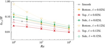
at different parts of the obstacles. In figure 9, the
 $\mathit{Ra}$
-scaling of
 ${\it\delta}_{T,i}$
for the two roughness configurations in comparison to the smooth case is presented. First of all, we observe that the thermal BL on top of the obstacles,
 ${\it\delta}_{T,top}$
, is the smallest and in particular it is smaller than that in the smooth case. Further,
 ${\it\delta}_{T,bottom}$
is larger than
 ${\it\delta}_{T,s}$
in the smooth case. This is in good agreement with the experimental results by Salort et al. (Reference Salort, Liot, Rusaouen, Seychelles, Tisserand, Creyssels, Castaing and Chillà2014). Also, for the slender obstacles,
 ${\it\delta}_{T,top}$
is smaller than for the wider ones. This is reasonable since the thermal BL thickness increases along the path of the wind (i.e. the large-scale circulation) (e.g. Wagner et al.
Reference Wagner, Shishkina and Wagner2012) and thus on average
 ${\it\delta}_{T,top}$
is expected to be smaller for slender obstacles with less distance along the wind on the obstacle top (cf. figure 6
d–f). Similarly,
 ${\it\delta}_{T,bottom}$
is larger for the wider obstacles, but here the explanation is different: wider obstacles lead to smaller distances
 $d_{x}$
between the obstacles, which makes it more difficult to wash out the warm fluid between the wider heated obstacles.
 $\mathit{Ra}$
-dependence of the thermal BL thickness,
 ${\it\delta}_{T,i}$
, at different parts of the rough surfaces (cf. text and figure 5) for roughness configurations
 $h=0.125H,\ell =0.025L$
(filled symbols, solid lines) and
 $h=0.125H,\ell =0.125L$
(open symbols, dotted lines) in comparison with the smooth case (crosses, dashed line).

Most interesting for understanding the influence of the roughness on the
 $\mathit{Ra}$
-dependence of
 $\mathit{Nu}$
is the fact that
 ${\it\delta}_{T,top}$
and
 ${\it\delta}_{T,side}$
scale similarly to the thermal BL thickness
 ${\it\delta}_{T,s}$
in the smooth case, and only the scaling of
 ${\it\delta}_{T,bottom}$
differs. This allows the interpretation that the ability of the flow to wash the warm fluid out of the cavities between the obstacles increases with increasing
 $\mathit{Ra}$
. The reason for this might be the fact that the typical size of the flow structures decreases with increasing
 $\mathit{Ra}$
, which makes it possible for the smaller structures to enter the cavities.
Further, for increasing
 $\mathit{Ra}$
, the thickness of the BLs decreases and thus the core part of the cavity enlarges, which aids the washing-out. Thus, exactly how the roughness influences the
 $\mathit{Ra}$
-scaling of
 $\mathit{Nu}$
depends on the combination of the size of the typical structures, determined by
 $\mathit{Ra}$
and
 $\mathit{Pr}$
, and the roughness configuration, i.e. the distance between the obstacles and the shape of the obstacles. Also, of course, the global flow structure, which depends on the geometry of the enclosure (Wagner & Shishkina Reference Wagner and Shishkina2013), might have an influence.
Thus we have found that the
 $\mathit{Ra}$
-scaling is similar for slender and wide obstacles (cf. figure 7
a), which can be explained by the similarity of the two configurations investigated. In the case of an even smaller distance between the obstacles (as in most experimental studies), the influence of the roughness might be much more strongly dependent on
 $\mathit{Ra}$
, since, e.g. for small
 $\mathit{Ra}$
, the warm fluid may permanently remain in the cavities.
Based on the above results, we conclude with respect the
 $\mathit{Ra}$
-scaling of
 $\mathit{Nu}$
as follows: the obstacles can lead to an increased scaling exponent. This increased exponent is connected to the ability of the flow to wash out the cavities between the obstacles, which depends on details of the roughness elements and the size of typical flow structures, i.e.
 $\mathit{Ra}$
. If washing-out is possible, i.e. here for large
 $\mathit{Ra}$
, the scaling exponent saturates to that of a smooth plate. This can be understood as a situation in which the roughness elements are covered by a thin thermal BL and work simply as an enlarged surface area. As discussed in the next section, this interpretation might be an explanation for the apparent differences between some experiments. Depending on details of the roughness in combination with the Rayleigh (and Prandtl) number, some experiments may find the increased scaling exponent, while others are in the parameter range at which the saturation takes place.
4. Limiting cases and theoretical model for the Nusselt number increase due to the roughness
Let us now analyse the theoretical limits of the heat flux increase due the presence of the roughness elements. Further, based on this analysis, we develop a simple model to estimate the behaviour of
 $\mathit{Nu}/\mathit{Nu}_{s}$
, in which the
 $\mathit{Nu}_{s}$
versus
 $\mathit{Ra}$
scaling parameters for the case of smooth top and bottom plates are used together with the geometrical characteristics of the cell with obstacles.
First we consider the case of the very thin obstacles with the width
 $\ell \rightarrow 0$
and the height much larger than the thickness
 ${\it\delta}_{T,s}$
of the thermal BL in the smooth case. We further assume that in this perfect case the obstacles are separated in such a way that there is no influence on the heat transfer from the vertical sides of any obstacle from the neighbouring obstacles. In this case one can use the Pohlhausen (Reference Pohlhausen1921) approximation to account for the contribution to the heat flux from the vertical surfaces of the roughness elements, in which the Nusselt number increase is proportional to the Rayleigh number, based on the height of the obstacles
 $h$
, taken to the power of
 $1/4$
. Thus, we obtain
 $$\begin{eqnarray}\mathit{Nu}/\mathit{Nu}_{s}=1+C(h/H)^{3/4}\end{eqnarray}$$
with a certain coefficient
 $C$
.
To estimate the coefficient
 $C$
, we further use the assumption that the Nusselt number increase due to the roughness, the height of which is smaller than the thermal BLs thickness, is directly proportional to the increase of the covering surface area of the top/bottom rough plates, i.e. the following holds:
 $$\begin{eqnarray}\mathit{Nu}/\mathit{Nu}_{s}=A/A_{s}.\end{eqnarray}$$
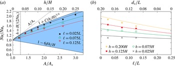
The regimes (4.1) and (4.2) should intersect when the roughness height is approximately equal to the thickness of the thermal BL in the smooth case (see figure 10
a). Taking into account that
 ${\it\delta}_{T,s}\approx H/(2\,\mathit{Nu}_{s})$
, one obtains
 $$\begin{eqnarray}C=\frac{A-A_{s}}{A_{s}}(2\,\mathit{Nu}_{s})^{3/4}\propto \mathit{Nu}_{s}^{3/4}.\end{eqnarray}$$
Thus, the upper bound of
 $\mathit{Nu}/\mathit{Nu}_{s}$
is given by (4.1) and (4.3).
Comparison of the DNS data (symbols) with the model (4.8), (4.9), (4.3),
 ${\it\beta}=0.3$
,
 $C=3.434$
(curves of the same shades as the corresponding symbols), for the relative increase of the Nusselt number due to the roughness,
 $\mathit{Nu}/\mathit{Nu}_{s}$
. The same data for
 $\mathit{Ra}=10^{7}$
are presented in two different ways: (a) as a dependence on the obstacle height
 $h$
, for some particular obstacle width
 $\ell$
and (b) as a dependence on the obstacle width
 $\ell$
, for some particular obstacle height
 $h$
. In (a) a vertical dashed line indicates the thickness of the thermal BL in the smooth case. The shaded domain shows the region of all possible values of
 $\mathit{Nu}/\mathit{Nu}_{s}$
, which is bounded by (4.1) for infinitesimally thin roughness elements, by (4.2) for the roughness height smaller than the thermal BL thickness in the smooth case and by (4.6) for infinitesimally thin cavities between the roughness elements.

For
 $\mathit{Ra}=10^{7}$
and
 $\mathit{Pr}=0.786$
our DNS gives
 $\mathit{Nu}_{s}=16.4$
(Wagner & Shishkina Reference Wagner and Shishkina2013) and thus
 $C\approx 3.343$
for the roughness configuration of four obstacles and the values of
 $\mathit{Ra}$
and
 $\mathit{Pr}$
considered. Note that for a fixed geometry of the convection cell and of the roughness elements introduced, the coefficient
 $C$
increases with the Nusselt number for the smooth case, and hence
 $C$
grows together with the Rayleigh number. The upper bound (4.1), (4.3) obtained for the ratio
 $\mathit{Nu}/\mathit{Nu}_{s}$
for
 $\mathit{Ra}=10^{7}$
,
 $\mathit{Pr}=0.786$
is seen in figure 10(a) as the upper boundary of the shaded region.
Further, a lower bound for the ratio
 $\mathit{Nu}/\mathit{Nu}_{s}$
(the lower boundary of the shaded region in figure 10
a) is obtained for the case of very wide obstacles, when
 $\ell \rightarrow L/n$
, where
 $n$
is the number of roughness elements introduced at each plate (in our DNS
 $n=4$
). In this limiting case there is no gap between the obstacles and the bottom (top) roughness elements form an isothermal solid heating (cooling) plate of thickness
 $h$
. The fluid is then confined between the plates, which are separated by a distance
 $H-2h$
. Since the effective Rayleigh number
 $\mathit{Ra}_{eff}$
of the resulting convection cell is
 $$\begin{eqnarray}\mathit{Ra}_{eff}\equiv \mathit{Ra}(1-2h/H)^{3}\leqslant \mathit{Ra},\end{eqnarray}$$
it is expected that the Nusselt number in this limiting case will be smaller than
 $\mathit{Nu}_{s}$
, according to the following relation:
 $$\begin{eqnarray}\mathit{Nu}/\mathit{Nu}_{s}=(1-2h/H)^{3{\it\beta}},\end{eqnarray}$$
where
 ${\it\beta}$
is the scaling exponent from
 $\mathit{Nu}_{s}\propto \mathit{Ra}^{{\it\beta}}$
. Here we assume that the change in the aspect ratio (length to height) of the fluid region from
 $L/H=1$
to
 $L/(H-2h)\geqslant 1$
does not affect the Nusselt number and its Rayleigh number dependence considerably. Numerical simulations for
 $\mathit{Pr}=0.7$
(Bailon-Cuba, Emran & Schumacher Reference Bailon-Cuba, Emran and Schumacher2010) and experiments in water (Zhou et al.
Reference Zhou, Liu, Li and Zhong2012) reveal only a weak influence of the aspect ratio. Our numerical simulations for
 $\mathit{Pr}=0.786$
give
 ${\it\beta}\approx 0.3$
in the
 $\mathit{Ra}$
-range considered. The relation (4.5) can be further simplified by considering only the linear term of a Taylor expansion for small
 $h/H$
, i.e.
 $$\begin{eqnarray}\mathit{Nu}/\mathit{Nu}_{s}\approx 1-6{\it\beta}h/H,\end{eqnarray}$$
which is presented in figure 10(a) as the lower boundary of the shaded region.
We introduce now the roughness density coefficient as follows:
 $$\begin{eqnarray}{\it\eta}\equiv n\ell /L,\end{eqnarray}$$
which is equal to zero in the first limiting case of infinitesimally thin obstacles and equal to one in the second limiting case of infinitesimally thin cavities between the obstacles. We seek an approximation of the Nusselt number enhancement due to the roughness in the form
 $$\begin{eqnarray}\mathit{Nu}/\mathit{Nu}_{s}=1+(B_{1}{\it\eta}+B_{2})(h/H)^{B_{3}{\it\eta}+B_{4}}\end{eqnarray}$$
with certain constants
 $B_{1}$
,
 $B_{2}$
,
 $B_{3}$
and
 $B_{4}$
. Since (4.8) should give (4.1) for
 ${\it\eta}=0$
and (4.6) for
 ${\it\eta}=1$
, we obtain
 $$\begin{eqnarray}B_{1}=-6{\it\beta}-C,\quad B_{2}=C,\quad B_{3}={\textstyle \frac{1}{4}},\quad B_{4}={\textstyle \frac{3}{4}}.\end{eqnarray}$$
The model (4.8), (4.9), (4.3) reflects the fact that the Nusselt number increase is larger for slender obstacles (
 ${\it\eta}$
is small) and for larger
 $\mathit{Nu}_{s}$
, i.e. for larger Rayleigh numbers.
In figure 10 we compare the DNS data with the model (4.8), (4.9), (4.3) in two different ways: as a dependence on
 $h$
(figure 10
a) and as a function of
 $\ell$
(figure 10
b), with other parameters fixed. We find a reasonable agreement of the theoretical and numerically obtained data. Note that the simple model (4.8), (4.9), (4.3) involves only geometrical characteristics of the convection cell with rough surfaces and the scaling of
 $\mathit{Nu}_{s}$
versus
 $\mathit{Ra}$
in the smooth case and allows further improvements by introducing additional parameters to fit.
5. Flow structure and velocity statistics
It is well known that in turbulent thermal convection of a fluid with
 $\mathit{Pr}\lesssim 1$
and large enough Rayleigh number, a large-scale circulation (wind) of the fluid develops in the bulk, i.e. the core part of the convection cell. This holds for both types of convection cells, with smooth and rough walls (see figure 2). The wind direction and its magnitude influence the flows that develop in the cavities between the isothermal roughness elements. In this section we discuss in more detail the wind and the cavity flows and related time-averaged characteristics, and analyse how they are influenced by a particular roughness geometry.
In RBC, the large-scale circulation of the fluid may reverse its direction (Sugiyama et al.
Reference Sugiyama, Ni, Stevens, Chan, Zhou, Xi, Sun, Grossmann, Xia and Lohse2010) on time scales of the order of the time used for temporal averaging in our DNS. If such a process takes place, time-averaged fields are strongly influenced and no longer represent the flow structure. To circumvent this, we consider only time intervals for averaging without such flow reversals. The latter information is obtained from instantaneous flow fields, saved with a sampling rate of four per time unit
 $(\widehat{H}/(\widehat{{\it\alpha}}\,\widehat{g}\widehat{{\it\Delta}}))^{1/2}$
. The instantaneous velocity field at half-depth is decomposed into several modes, as described in detail by Wagner & Shishkina (Reference Wagner and Shishkina2013) and similarly by Chandra & Verma (Reference Chandra and Verma2013). The time histories of the contributions of these modes are then used to evaluate the direction of the large-scale flow.
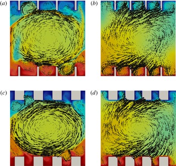
In figure 11 the time-averaged temperature distributions with superposed velocity vectors are presented for two particular roughness configurations:
 $h=0.125H$
and
 $\ell =0.025L$
or
 $\ell =0.125L$
, as obtained in the two-dimensional DNS for
 $\mathit{Pr}=1,\mathit{Ra}=10^{8}$
(Shishkina & Wagner Reference Shishkina and Wagner2011) and in the present three-dimensional DNS for
 $\mathit{Pr}=0.786,\mathit{Ra}=10^{7}$
, in the central vertical cross-section. In the two-dimensional case (figure 11
a,c) one observes an almost circular movement of the fluid, while in the three-dimensional case (figure 11
b,d) the wind exhibits its three-dimensional spiral structure. Thus in the three-dimensional case the fluid can move along the obstacles, in the direction orthogonal to the cross-sections presented in figure 11(b,d). Such a fluid motion aids the emission of the thermal plumes from the heated surfaces of the roughness elements, and as a result the wind can remove more heat from these surfaces than in the two-dimensional case.
Time-averaged temperature distributions with superposed randomly distributed velocity vectors for different roughness configurations: (a,b)
 $h=0.125H,\ell =0.025L$
; (c,d)
 $h=0.125H,\ell =0.125L$
as obtained in: (a,c) two-dimensional DNS for
 $\mathit{Ra}=10^{8},\mathit{Pr}=1$
(Shishkina & Wagner Reference Shishkina and Wagner2011), and (b,d) three-dimensional DNS for
 $\mathit{Ra}=10^{7},\mathit{Pr}=0.786$
, in the vertical slice at half-depth. Colour scale goes from blue (
 $\widehat{T}_{top}$
) to red (
 $\widehat{T}_{bottom}$
) and the length of the vectors represents the magnitude of the in-plane velocity at the arrow tails.

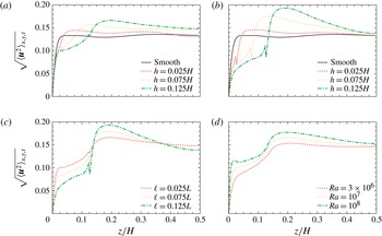
To analyse the effect of the regular roughness on the large-scale circulation and the flows between the obstacles, we evaluate the time-averaged vertical profiles of the velocity magnitude, which are presented in figure 12. Close to the bottom plate, for
 $z\leqslant h$
, the averaging is performed only for the fluid regions, while above the roughness elements, for
 $z>h$
, the profiles are averaged over the whole horizontal cross-section. Figure 12(a–c) reveals that the wind is always stronger than the mean secondary flow in the cavities between the obstacles. If for a fixed Rayleigh number a certain change of the geometry (the obstacle height or width) leads to a decrease (or increase) in the velocity magnitude of the secondary flow, then in contrast, the magnitude of the wind increases (or decreases).
Vertical profiles of the time and spatially averaged velocity magnitude
 $\sqrt{\langle \boldsymbol{u }^{2}\rangle _{x,y,t}}$
. For
 $z\leqslant h$
the averaging in the
 $x$
-direction is performed only over the fluid regions, which leads to discontinuities at
 $z=h$
. Profiles for: (a)
 $\ell =0.025L$
and (b)
 $\ell =0.125L$
and different
 $h$
; and (c) for
 $h=0.125H$
and different
 $\ell$
, with
 $\mathit{Ra}=10^{7}$
. (d)
 $\mathit{Ra}$
-dependence of the profiles for
 $h=0.025H$
and
 $\ell =0.125L$
.

From the comparison of the profiles for
 $\mathit{Ra}=10^{7}$
in the cases of slender obstacles (figure 12
a,
 $\ell =0.025L$
) and wide obstacles (figure 12
b,
 $\ell =0.125L$
), we conclude that the secondary flow is generally stronger if the distance between the roughness elements is large enough, i.e. the obstacles are slender, while the wind close to the upper boundaries of the obstacles is stronger for wide obstacles. This is consistent with the fact that in turbulent thermal convection, the wind accelerates along its path, close to the heated surfaces (Kaczorowski et al.
Reference Kaczorowski, Shishkina, Shishkin, Wagner, Xia, Kuerten, Geurts, Armenio and Fröhlich2011; Wagner et al.
Reference Wagner, Shishkina and Wagner2012); therefore the presence of wide roughness elements generally leads to a stronger wind above them.
If the Rayleigh number and the height of the regular roughness are fixed and the width of the obstacles is varied, the mean vertical profiles of the velocity magnitude reveal three main regions of the dominance of different trends activated by the roughness, as depicted in figure 12(c). In the first region, within the cavities between the obstacles, the mean flow is stronger for slender obstacles that retain enough space between them. In the second region, which extends from the upper boundaries of the obstacles to about one-third of the convection cell, the wind is stronger for wider roughness elements. Finally, in the core region of the convection cell, the wind is generally stronger for slender obstacles.
Probability density function of the velocity magnitude in comparison with the smooth case (Wagner & Shishkina Reference Wagner and Shishkina2013) for: (a) different obstacle heights and
 $\ell =0.025L$
,
 $\mathit{Ra}=10^{7}$
; (b)
 $h=0.125H$
and different
 $\ell$
,
 $\mathit{Ra}=10^{7}$
; (c)
 $h=0.125H$
,
 $\ell =0.025L$
and different
 $\mathit{Ra}$
. For the rough cases, the PDFs are taken separately for the bulk region, i.e.
 $h<z<H-h$
and the cavity region, i.e.
 $0\leqslant z\leqslant h$
and
 $h-H\leqslant z\leqslant H$
.

It should be noted that for the non-dimensionalisation, the reference velocity
 $\sqrt{\widehat{{\it\alpha}}\,\widehat{g}\widehat{{\rm\Delta}}\widehat{H}}\sim \sqrt{\mathit{Ra}}$
has been used. Thus, when comparing the results for different Rayleigh numbers in figure 12(d), the increase in all regions means that the velocities increase more rapidly than
 $\sqrt{\mathit{Ra}}$
.
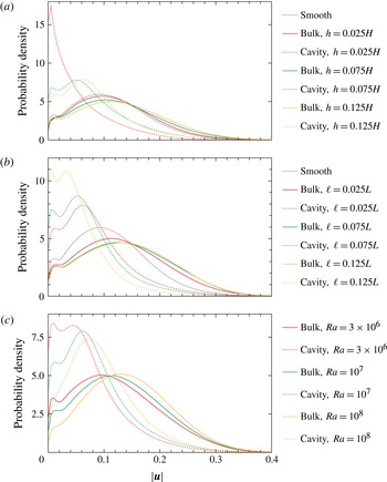
The trends described above are also supported by the analysis of the time-averaged probability density functions (PDFs) of the local instantaneous velocity magnitude
 $|\boldsymbol{u}|$
. The probability density functions are evaluated separately for the cavity regions between the obstacles and the remaining core part of the convection cell, as presented in figure 13. For a fixed Rayleigh number and fixed width of the roughness elements (figure 13
a,
 $\mathit{Ra}=10^{7}$
,
 $\ell =0.025L$
) the most probable velocity increases both in the cavity and in the bulk, if the height of the obstacles is increased. In the case of a fixed Rayleigh number and fixed height of the roughness elements and varying obstacle width (figure 13
b,
 $\mathit{Ra}=10^{7}$
,
 $h=0.125H$
), the trends in the cavities and in the bulk are opposite: with increasing
 $\ell$
, the most probable velocity in the cavities decreases, while that in the bulk increases. As already discussed above, an increase in the obstacle width impedes the development of strong secondary flow structures between the roughness elements but favours the acceleration of the wind above the obstacles. Finally, an increase in the Rayleigh number (figure 13
c) always leads to an increase in the most probable velocity, both in the cavity and in the bulk regions.
6. Detailed comparison with the literature
In the following we compare the general results of the present DNS against different models and results for the heat flux enhancement by roughness in the literature.
6.1. The two-dimensional model by Shishkina & Wagner (Reference Shishkina and Wagner2011)
First we compare the results obtained with the those from the model by Shishkina & Wagner (Reference Shishkina and Wagner2011) for heat flux enhancement due to distinct regularly distributed obstacles. The main idea of that model is the decomposition of the total heat flux into the three contributions
 $Q_{top}$
,
 $Q_{bottom}$
,
 $Q_{side}$
introduced above, which are modelled separately. The main assumptions of this model are stationary BLs, which can be well described by the theory of Prandtl–Blasius and Pohlhausen (see e.g. Shishkina et al.
Reference Shishkina, Stevens, Grossmann and Lohse2010), and obstacles which are much larger than the thermal BL thickness
 $H/(2\,\mathit{Nu}_{s})$
. The model is two-dimensional by construction and shows good agreement with DNS results of two-dimensional RBC for
 $\mathit{Pr}=1$
and
 $\mathit{Ra}\in \{10^{7},5\times 10^{7},10^{8}\}$
and roughness configurations similar to those in the present study.
Due to the fact that the obstacles in the present paper are uniform in the
 $y$
-direction, i.e. the additional direction compared to the two-dimensional study, the model does not need to be extended for a comparison with the present three-dimensional DNS results. For the special case of four obstacles it is modelled that
 $(Q_{top}+Q_{bottom})/(\mathit{Nu}_{s}A_{s})\approx 1/4+(3/4)(H_{esw}/H)$
and
 $Q_{side}/(\mathit{Nu}_{s}A_{s})\approx 2^{11/4}{\it\xi}^{1/4}h^{7/4}L^{-1}H^{-3/4}$
, such that
 $\mathit{Nu}\,A_{s}=\sum _{i}Q_{i}$
. Here
 $H_{esw}=H-8\ell h/L$
is the ‘equivalent-smooth-wall height’ introduced in § 3.2. Further,
 ${\it\xi}$
is the obstacle rarity coefficient, which is defined as
 ${\it\xi}=b\,d_{x}/h$
for
 $b\,d_{x}/h<1$
and
 ${\it\xi}=1$
for
 $b\,d_{x}/h\geqslant 1$
.
First, it should be noted that the two-dimensional model does not predict the increased scaling exponent due to roughness by construction, which is observed in the present DNS results, in particular for
 $\mathit{Ra}\leqslant 10^{7}$
. Since the scaling exponent seems to saturate for very large
 $\mathit{Ra}$
to the scaling observed in the smooth case, the model may perform better at that point when considering
 $\mathit{Ra}\gg 10^{8}$
.
For fixed
 $\mathit{Ra}$
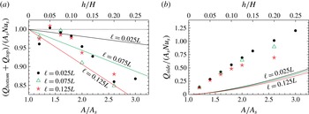
a quantitative comparison of the model with DNS results is presented in figure 14, where the heat flux predictions of the model for the horizontal (
 $Q_{top}+Q_{bottom}$
) and vertical surfaces (
 $Q_{side}$
) are compared with the three-dimensional DNS results for
 $\mathit{Ra}=10^{7}$
.
Comparison of the predictions by Shishkina & Wagner (Reference Shishkina and Wagner2011) with the DNS results for the heat flux from (a) the horizontal surfaces
 $Q_{top}+Q_{bottom}$
and (b) the vertical surfaces
 $Q_{side}$
for
 $\mathit{Ra}=10^{7}$
. The solid lines represent the model predictions and the symbols the DNS, for different widths of the obstacles
 $\ell$
.

As depicted in figure 14(a), the model cannot reproduce more than the correct order of magnitude of the deviation from the smooth case (indicated by a horizontal dotted line) when comparing the contributions from the horizontal surfaces. With respect to
 $Q_{side}$
in figure 14(b), the model strongly underestimates the DNS results, which in total leads to a strongly underpredicted total heat flux enhancement by the roughness.
The reason for this underestimation might be the assumption of the Pohlhausen theory for infinite vertical heated surfaces (Pohlhausen Reference Pohlhausen1921; Landau & Lifshitz Reference Landau and Lifshitz1987), which neglects the occurrence of thermal plumes. The latter are present in particular at the obstacle edges (Du & Tong Reference Du and Tong2000; Stringano et al. Reference Stringano, Pascazio and Verzicco2006). Furthermore, the uplift next to the vertical walls of the obstacles is expected to be only caused by buoyancy, i.e. driven by the temperature gradient next to the vertical wall. This estimate might lead to velocities that are far too small, since the flow between the obstacles is also partly driven by the large-scale circulation in the full cell.
Further, the global flow structures in the core parts of the convection cells differ in the two- and three-dimensional cases, which also influences the processes of washing-out of the fluid from the cavities between the isothermal roughness elements.
6.2. The experimental results by Salort et al. (Reference Salort, Liot, Rusaouen, Seychelles, Tisserand, Creyssels, Castaing and Chillà2014)
Salort et al. (Reference Salort, Liot, Rusaouen, Seychelles, Tisserand, Creyssels, Castaing and Chillà2014) conducted experiments in a box-shaped container as in the present numerical study. The container was filled with water (
 $3.9\leqslant \mathit{Pr}\leqslant 8.1$
) and regular roughness was introduced at the bottom plate by square studs with height
 $h\approx 0.005H$
and
 $\ell =d_{x}=0.0125L$
(in both horizontal directions). The top plate was left smooth to allow in situ comparison of the flow with and without roughness elements (see also Tisserand et al.
Reference Tisserand, Creyssels, Gasteuil, Pabiou, Gibert, Castaing and Chillà2011). Since the Rayleigh number was varied in the range
 $10^{9}{-}10^{11}$
, the thickness of the thermal BL (computed from the Nusselt numbers for smooth plates) varied between
 ${\it\delta}_{T}\approx 3.3h$
and
 ${\it\delta}_{T}\approx 0.77h$
. They observed for
 $\mathit{Ra}$
large enough, i.e.
 ${\it\delta}_{T}\lesssim h$
, an increased scaling exponent caused by roughness. Furthermore, they performed local temperature measurements between and on top of the roughness elements at different distances from the plate for a fixed Rayleigh number. From these measurements they deduced that in so-called notches, i.e. cavities similar to the ones in the present paper, the temperature fluctuations are weak. Salort et al. (Reference Salort, Liot, Rusaouen, Seychelles, Tisserand, Creyssels, Castaing and Chillà2014) conclude that the notches do not contribute significantly to the total heat flux. In addition, on top of the roughness elements, the thermal BL was found to be much thinner than in the case of a smooth plate. They conclude that the BL on top of the obstacles can be understood as a fully turbulent one, which then leads to an increased scaling exponent.
Comparison to the present DNS results reveals some similarities. We also obtain that the thickness of the thermal BL on top of the roughness elements is much thinner than in the smooth case, but it does not scale in a different way with respect to
 $\mathit{Ra}$
. This result was not obtained from their experiments, as they measured the thickness only for a fixed
 $\mathit{Ra}$
. In the experiments it was additionally found that the temperature field inside the notches was not fluctuating much, which could be interpreted as an insufficient washing-out of the cavities between the obstacles. Thus, the experiments presumably could not reach sufficiently large
 $\mathit{Ra}$
(which is expected to be much larger than in our DNS, since the distance between the roughness elements was much smaller in the experiments) to obtain the saturation in the
 $\mathit{Nu}$
versus
 $\mathit{Ra}$
scaling as in our DNS.
6.3. The experimental results by Du & Tong (Reference Du and Tong1998, Reference Du and Tong2000)
Du & Tong (Reference Du and Tong1998, Reference Du and Tong2000) performed experiments in cylindrical containers with aspect ratio (
 ${\it\Gamma}=\text{diameter}$
/height) equal to
 $1/2$
and 1, filled with water (
 $\mathit{Pr}\approx 5.4$
). In addition to smooth heating and cooling plates, they conducted experiments with square-based pyramids of height
 $h=0.045H~({\it\Gamma}=1)$
and
 $h=0.0225H~({\it\Gamma}=1/2)$
as roughness elements. The spacing between the roughness elements was
 $2h$
. An additional rough plate with smaller roughness elements of height
 $h=0.016H~({\it\Gamma}=1)$
and the same surface structure was also used in their experiments. Only for the smallest obstacles was the obstacle height similar to the thickness of the thermal BL in the smooth case at the lowest
 $\mathit{Ra}$
studied. The higher obstacles were thus always much larger than the thickness of the thermal BL. Du & Tong (Reference Du and Tong1998, Reference Du and Tong2000) report an increase of the global heat flux which is different for different plates, but does not show an increased scaling exponent over two decades in
 $\mathit{Ra}$
. Only for the small obstacles and the lowest Rayleigh numbers of approximately
 $10^{9}$
, i.e. the thermal BL has a thickness of approximately
 $0.0077H$
, was a weak trend towards an increased scaling exponent observed. In addition to the heat flux, local temperature measurements and flow visualisations with thermochromatic liquid crystals were also conducted. Both reveal a washing-out of the cavities between the obstacles by secondary flows, which is driven by the large-scale flow in the bulk region of the container. This fact suggests that the experiments were conducted in the parameter range in which a saturation of the
 $\mathit{Nu}$
versus
 $\mathit{Ra}$
scaling might be observed. In the case of the small obstacles and small
 $\mathit{Ra}$
, i.e. a parameter combination for which the washing-out is most difficult, an increased scaling exponent as in the present DNS study was observed. Thus, it can be deduced that the experiments of Du & Tong (Reference Du and Tong1998, Reference Du and Tong2000) are not in contradiction to experiments and simulations showing an increased scaling exponent, since they are simply conducted under different conditions.
7. Conclusions
DNS of the turbulent thermal convection in parallelepipedal domains with rough heated and cooled surfaces were conducted, in which the width, height and depth of the domains are related as 1:1:0.25. In all the simulations, the Prandtl number is equal to
 $\mathit{Pr}=0.786$
, while the Rayleigh number
 $\mathit{Ra}$
varies between
 $10^{6}$
and
 $10^{8}$
. The surface roughness is introduced by four box-shaped equidistantly distributed obstacles attached to the heating bottom plate and four obstacles located symmetrically on the cooled top plate.
The effect of the roughness was investigated in two ways: first, for a fixed Rayleigh number (
 $\mathit{Ra}=10^{7}$
) and changing roughness configurations and, second, for fixed roughness types, while varying the Rayleigh number.
As in the two-dimensional study of Shishkina & Wagner (Reference Shishkina and Wagner2011), we found that a relative increase in the covering area of the heated/cooled surfaces is not a universal parameter that determines the relative change of the mean heat flux measured by the Nusselt number. Our three-dimensional DNS showed that if the distance between the obstacles is large enough, an almost linear increase of the Nusselt number with the covering area remains longer for slender obstacles, which helps the fluid stagnating between the isothermal obstacles to be washed out from the cavities from time to time. Our DNS results in the parameter range considered are well represented by the empirical function (3.2) presented in this paper to estimate the heat flux increase due to roughness.
Based on theoretical limiting cases for slender and very wide obstacles, a simple model (4.8), (4.9), (4.3) was built. Even though the model does not require any adjustment of free parameters, it still can reproduce the general trends obtained in the DNS results. Further, the right order of magnitude of the heat flux enhancement found in the DNS for the parameter range considered can be predicted by the simple model.
The three-dimensional DNS results were also compared with the two-dimensional model of Shishkina & Wagner (Reference Shishkina and Wagner2011), which was found to underestimate the heat flux from the vertical walls of the obstacles. The deviation obtained is explained by the essential three-dimensionality of turbulent convective flows, and by the fact that the flows in the cavities between the isothermal obstacles are caused not only by buoyancy but also by the large-scale circulation of the fluid in the core part of the convection cell. For similar configurations of regular roughness, the structure of the large-scale circulation in the two-dimensional and three-dimensional convective flows are also different: in the three-dimensional case the wind exhibits a three-dimensional spiral-like structure, which improves the heat transport from the rough surfaces.
The analysis of the local thermal BL thickness showed that the thinnest BL develops at the top of the obstacles, and for similar
 $\mathit{Ra}$
and
 $\mathit{Pr}$
it is always smaller than the BL thickness in the case of a smooth heated/cooled surface. The thickness of the thermal BL at the top of the obstacles is especially small for slender roughness elements. In contrast to the BLs attached to the obstacle tops, the BLs near the bottom or vertical sides of the obstacles are always thicker than those in the case of a smooth heated/cooled surface.
For two particular roughness configurations, with slender and wide obstacles but the same covering area of the surfaces (
 $\ell =0.025L$
,
 $h=0.125H$
and
 $\ell =0.125L$
,
 $h=0.125H$
), the effect of the roughness on the
 $\mathit{Nu}$
versus
 $\mathit{Ra}$
scaling was investigated. It was found that the global scaling exponent changes from approximately 0.31 for smooth walls to approximately 0.37 for both types of rough wall. Again, the strongest effect was observed for the slender roughness elements. A closer look showed that the largest value of the exponent, approximately 0.40, corresponds to smaller Rayleigh numbers, about
 $\mathit{Ra}\approx 10^{6}$
, while for
 $\mathit{Ra}>10^{7}$
it reduces and tends to the one obtained for smooth plates for
 $\mathit{Ra}\approx 10^{8}$
especially for wide roughness elements. The analysis of the
 $\mathit{Nu}$
versus
 $\mathit{Ra}$
scaling with respect to the so-called ‘equivalent-smooth-wall height’
 $H_{esw}$
led to the same result. The thickness of the thermal BL at different parts of the roughness elements scales generally in a similar way, both for rough and smooth surfaces. Only at the bottom of the cavities between the obstacles is the scaling exponent found to be different for small Rayleigh numbers. Thus, the scaling exponent for rough plates is only affected by this region. In addition the thermal BL in this region of the rough plate is thicker than in the case of a smooth plate. Therefore, the increased scaling exponent is present because of an insufficient ventilation of the cavities at low
 $\mathit{Ra}$
for which the thermal BL is generally thicker than for larger
 $\mathit{Ra}$
. For higher
 $\mathit{Ra}$
the ventilation of the cavities is easier and the scaling exponent becomes similar to the one for smooth plates. Thus, the increased scaling exponent might just be present in an
 $\mathit{Ra}$
-range for which:
-
(a) the height of the obstacles
$h$
is larger than the thickness of the thermal BL in the case of smooth plates; -
(b) the cavities between the obstacles are not fully washed out, which may depend on the obstacle height, the distance between the obstacles,
$\mathit{Ra}$
,
$\mathit{Pr}$
and the shape of the roughness elements.


Keeping this idea in mind there might be an explanation for the apparent differences between experiments with respect to the influence of roughness on the scaling of
 $\mathit{Nu}$
. We discussed in particular the results by Du & Tong (Reference Du and Tong1998, Reference Du and Tong2000) and Salort et al. (Reference Salort, Liot, Rusaouen, Seychelles, Tisserand, Creyssels, Castaing and Chillà2014). While Du & Tong (Reference Du and Tong1998, Reference Du and Tong2000) observed fully ventilated cavities and no effect on the scaling exponent, Salort et al. (Reference Salort, Liot, Rusaouen, Seychelles, Tisserand, Creyssels, Castaing and Chillà2014) found stagnating fluid between the obstacles and an increased scaling exponent. It should be further noted that the model (Villermaux Reference Villermaux1998) proposed an unaffected scaling exponent for regular roughness under the assumption of fully ventilated cavities. We do not claim that this is the final explanation for the differences between the different experiments, but we suggest that not only the obstacle height but also the distance between the obstacles in combination with
 $\mathit{Ra}$
should be taken into account when comparing the results of different experiments.
A comparison of the time-averaged vertical profiles of the kinetic energy for different roughness configurations showed that the mean secondary flow in the cavities between the obstacles and the wind, which is always stronger than these secondary flows, are related and can be influenced by the geometry of the regular roughness in such a way that the strengthening (weakening) of one of them leads to the weakening (strengthening) of the other. Thus, wide obstacles impede the flow between them but contribute to the acceleration of the large-scale circulation.
Generally, the growth of the roughness height leads to stronger flows both in the cavities and in the bulk region, while an increase in the obstacle width accelerates only the large-scale circulation of the fluid and decelerates the secondary flows between the roughness elements. Any increase in the Rayleigh number leads to stronger flows, both in the cavities and in the bulk.
Further investigations of the influence of regular roughness on the heat and mass transfer in natural convection are needed, in particular issues related to the dependence on the Prandtl number and the Rayleigh number for large
 $\mathit{Ra}$
. The development of a model to predict the heat flux enhancement due to regular wall roughness that takes into account the three-dimensionality of the flows and the influence of the wind on the secondary flows between the obstacles should also be addressed in the future.
Acknowledgements
We are grateful to one of the unknown referees for suggesting that we consider the limiting cases of
 $\mathit{Nu}/\mathit{Nu}_{s}$
; this prompted us to develop a simple model in § 4. Further, we acknowledge financial support by the German Research Foundation (DFG) under the grant SH405/3-1 and the Heisenberg fellowship SH405/4-1.