I. INTRODUCTION
CALPHAD (CALculation of PHAse Diagrams) methodReference Kaufman and Cohen1–Reference Saunders and Miodownik3 is “a way to encode experimental and theoretical results in a thermodynamic language to make them applicable to a much wider context than original experiments or calculations.”Reference Kaufman and Agren4 CALPHAD is founded on thermodynamic principles formulated by Gibbs.Reference Gibbs5 The Gibbs energy functions describing a system are indirectly obtained from experimental, and sometimes first principles, information. Thermodynamic descriptions of several low-order systems can be appended together to describe multicomponent higher-order systems. Using these CALPHAD databases, Gibbs energy minimizer codes, such as ThermoCalc,Reference Sundman, Jansson and Andersson6 MTDATA,Reference Dinsdale, Hodson and Taylor7 and PANDAT,Reference Chen, Daniel, Zhang, Chang, Yan, Xie, Schmid-Fetzer and Oates8 enables the performance of calculations in complex systems and map the equilibrium states as a function of the thermodynamic conditions even where data are not available. This predictive capability of computational thermodynamics (e.g., CALPHAD) represents a powerful material engineering tool that takes on its full interest, but also faces a challenge, for the development of multicomponent alloys such as the so-called high entropy alloys (HEAs) and related alloy concepts.
Depending on definitions, HEAs consist of at least four or five principal elements (they are baseless) with equivalent concentrations which place them in the central, often uncharted, regions of multidimensional composition spaces. Due to the a priori unexpected single-phase microstructures reported in the early papers,Reference Cantor, Chang, Knight and Vincent9,Reference Yeh, Chen, Lin, Gan, Chin and Shun10 the emphasis was put on the role of configurational entropy—from where their name comes—, to explain the stability of disordered solid solutions in these multiprincipal element alloys. Then, HEA studies became mainly motivated by the search of the quinary equimolar disordered solid solution phase giving little considerations to the attractiveness of single-phase microstructures with respect to the mechanical properties. The rational was based on four hypothetical effects associated with HEAsReference Yeh11: the high entropy effect, the lattice distortion effect, the sluggish diffusion, and the “cocktail” effect. However, over the last years, the few studies that have examined these core effects do not fully support all these claims.Reference Pickering and Jones12 In addition to these concepts, interesting properties could be envisioned due to the single-phase microstructure, like good ductility and corrosion resistance due to the absence of secondary phases at grain boundaries. Recently, several players of the HEA community returned to the major founding concept that is related to the vastness and still unexplored interior regions of higher-order phase diagrams, and to the basics of the metallurgy that is the design and genesis of microstructures.Reference Miracle13 In the following, we use the term HEA to designate single-phase solid solution microstructures and CCAs (complex concentrated alloys) to describe multiphase microstructures. CCAs offer unprecedented degrees of freedom to design advanced microstructures with improved properties. The number of alloy chemistries and thermomechanical treatments that can be combined are almost infinite, and the probability of finding the optimum solution is negligible through trial-and-error. Alloy designers need predictive tools to rapidly investigate the composition space and evaluate the effects of element concentration and temperature on phase stability and the resulting microstructure.
In the present paper, we will first discuss the concept of entropy-stabilized single solid solution through statistical and thermodynamic analysis to assess the role of entropy on phase stability. We will then provide some short reviews of studies and original results related to the practices of the CALPHAD approach applied to explain experimental observations under both equilibrium and nonequilibrium situations. The reliability of CALPAHD predictions will be briefly addressed too. Then, we will discuss the future role of CALPHAD as a major part of the development of the new generation of HEAs and CCAs. Finally we will introduce guided exploration strategies of the compositional space that can dramatically accelerate the discovery and development of HEAs and CCAs with improved performance.
II. CROSSED PERSPECTIVE ON HEAS: STATISTICAL AND THERMODYNAMIC POINT OF VIEW
In this section, we will give a brief overview of the current landscape of HEAs and CCAs and discuss the hypothesis of entropy-stabilized alloys based on statistical analysis of the experimental observations and thermodynamic considerations regarding the role of entropy on the Gibbs energy and phase stability.
A. Fly over the current landscape of HEAs and CCAs
1. Iconic HEAs
The approach being explored within HEAs states that increasing the number of elements and favoring equimolar compositions increase the configurational entropy (this will be explained later), decrease the Gibbs free energy of a disordered solid solution, and stabilize it over other competing phases. Such a strategy has been largely implemented in the hope of obtaining single solid solutions in many multiprincipal element alloys. Numerous materials have been elaborated and tested according to the above rules. The following list gives examples of experimentally reported alloys exhibiting single disordered solid solution at equimolarity: AlCoCuNiTiZn,Reference Varalakshmi, Kamaraj and Murty14 AlCrCuFeMnNi,Reference Chen, Tsai, Tung, Yeh, Shun, Yang and Chen15 AlNbTaTiV,Reference Yang, Zhang and Liaw16 CoCrCuFeMnNi,Reference Cantor, Chang, Knight and Vincent9 CoCrCuFeNi,Reference Yeh, Chen, Lin, Gan, Chin and Shun10 CoCrFeMnNi (usually known as “Cantor alloy”),Reference Cantor, Chang, Knight and Vincent9 CoCuFeNiV,Reference Zhang, Zhou, Lin, Chen and Liaw17 CrCuFeMoNi,Reference Li, Li, Zhao and Jiang18 DyGdHoTbY,Reference Feuerbacher, Heidelmann and Thomas19 DyGdLuTbTm,Reference Takeuchi, Amiya, Wada, Yubuta and Zhang20 DyGdLuTbY,Reference Takeuchi, Amiya, Wada, Yubuta and Zhang20 HfMoNbTiZr,Reference Guo, Wang, Luo, Li, Su, Guo and Fu21 HfNbTaTiZr,Reference Senkov, Scotta, Senkova, Miracle and Woodward22 MoNbTaVW,Reference Senkov, Wilks, Miracle, Chuang and Liaw23 and MoNbTiVZr.Reference Zhang, Yang and Liaw24
2. Deviant HEAs
Nevertheless, the scientific literature also reports several nonequimolar multiconcentrated alloys forming a single solid solution, i.e., nonequimolar HEAs. In fact, more of them have been reported than equimolar HEAs, although their configurational entropy is lower. Among others, there are a few examples where the nonequimolar alloy is single phased, whereas its equimolar counterpart is not, which was noticed early in the HEA development history, e.g., with Al2.8CoCrCuFeNi versus AlCoCrCuFeNi,Reference Yeh, Chen, Lin, Gan, Chin and Shun10 although the configurational entropy of the former is lower than that of the latter. The same remark holds when comparing the equimolar HEA CoCrFeMnNi with a nonequimolar HEA of the same family, Co20Cr15Fe26Mn17Ni22, the latter displaying a larger temperature range of stability of the single solid solution,Reference Mroz25 although having a lower configurational entropy.
3. HEAs versus CCAs
Two databases containing more than 300 multiconcentrated alloys each have recently been compiled and published by Gorsse et al.Reference Gorsse, Miracle and Senkov26 and Toda et al.,Reference Toda-Caraballo and Rivera-Díaz-del-Castillo27 respectively.
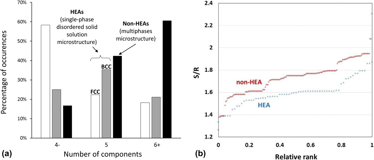
Gorsse’s database has a tree-like classification with five CCA/HEA families (3d transition metals, refractory metals, light weight, brasses & bronzes, and 4d lanthanide CCAs). Each family is expanded to show classes (one class is a unique combination of principal elements), each class contains members having variations in principal element concentrations, and finally each member is characterized by a set of attributes. This database contains more than 300 alloys with their composition, phases—i.e., solid solutions (FCC, BCC, and HCP), ordered phases, and intermetallics—and their mechanical and functional properties. Figure 1(a) displays a microstructure classification by phase types as a function of the number of components entering the alloy compositions. The occurrence of non-HEAs (multiphase microstructures) increases with the number of components, whereas the number of HEAs (single-phase disordered solid solution microstructures) decreases, which contradicts the high entropy hypothesis, i.e., entropic stabilization of a single-phase disordered solid solution when the number of components increases.
(a) Occurrence of HEAs and non-HEAs as a function of the number of elements; (b) cumulative distribution of the configurational entropy of HEAs and non-HEAs.

Toda’s database contains several tens of HEAs, i.e., forming a single solid solution, as well as many non-HEAs constituted of mixtures of solid solutions, intermetallics, mixtures of a solid solution with intermetallics, etc. These data are here analyzed by calculating the raw configurational entropy (see section II.C) of all alloys, ranking alloys of each category (HEAs and non-HEAs) by ascending order of configurational entropy, normalizing the rank in each category between 0 and 1 for comparison purposes, and finally plotting the cumulative distribution of configurational entropies as on Fig. 1(b). Obviously, for real alloys, non-HEAs exhibit overall a larger configurational entropy than HEAs.
Both these analyses show that configurational entropy, if it may contribute to the obtainment of HEAs, is clearly not the major parameter governing the formation of a single solid solution in multiconcentrated alloys. Two other reviews have come to the same conclusion.Reference Pickering and Jones12,Reference Miracle and Senkov28
B. Statistics do not like HEAs
1. Solid solution versus all the rest
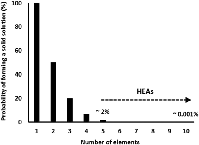
The “high entropy approach” exposed in early papers is in fact partly appropriate only, on the one hand because it would consider the sole configurational entropy (this will be discussed later), and on the other hand because it would consider only the decrease in Gibbs free energy, due to the increase in entropy, of the sole solid solution. However, the formation of a phase does not require that its free energy is low, but it needs to be lower than that of all other potential phases. When the number of elements increases, the number of potential phases increases faster, hence the number of possible constitutions concurrent to a single solid solution so that the “competition” becomes statistically ruder and ruder for the solid solution. It is impossible to calculate an exact number of possible phases or constitutions that would hold for any alloy system because it depends on each system, but an illustrative combinatorial approach can help to provide an order of magnitude of the problem. For instance, with one element, a single phase is necessarily formed. With two elements, say A and B, in equimolar proportions, a single phase AB can form or a decomposition in two phases A + B can occur (these could be solid solutions rich in A or B; besides the phase AB could well be a solid solution or an intermetallic, and several intermetallics AmBn could exist, which would increase the potential number of phases and constitutions, but let us make things simple: this way the model will be quite “optimistic” for HEA formation). Two constitutions can thus exist (AB or A + B) so that the probability of forming a single phase (AB) is 50%. Of course, this reasoning is purely combinatorial and not physical, but it may show trends. With three elements, say A, B, and C, one can form a single phase ABC or decompose the alloy in several phases: A + B + C, or A + BC, or B + AC, or C + AB. This makes five possible constitutions so that the probability of forming a single phase drops to 20%. And so forth when the number of elements is increased. The counting of all possible constitutions, i.e., of different manners of decomposing a set of N elements in subsets, uses Bell’s numbers.Reference Crepain29 The first ten Bell’s numbers, i.e., for N from 1 to 10, are 1, 2, 5, 15, 52, 203, 877, 4140, 21,147, and 115,975. The probability of forming a single phase for a given number of alloying elements can thus be thought to be equal to the inverse of these numbers. This is plotted in Fig. 2.
Probability of forming a single phase as a function of the number of alloying elements.

Once more, this model is simplistic but it gives a picture of the competition that a solid solution has to face when the number of elements increases. For instance, with five elements, which is the usual minimum number of elements considered necessary to produce a HEA, the probability is less than 2%. It becomes less than 0.5% for six elements, ∼0.1% for seven elements, and goes down to less than 0.001% for ten elements. Another consequence of this result is that single-phase HEAs may in fact be rare among multicomponent concentrated alloys; this will be discussed later. Also, this competition between the formation of a single solid solution and other constitutions will be expressed later in a rigorous manner using the CALPHAD approach.
2. Solid solution versus intermetallics
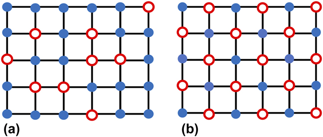
As stated earlier, the obtainment of a HEA depends on the competition between the solid solution and all other possible phases. A particularly interesting case is that of intermetallics. Indeed, their configurational entropy is very low—it is even null for a fully ordered phase since there is only one possible configuration. At the opposite, whereas in disordered solid solutions the neighborhood of a given atom is randomly made of other alloying elements so that the number of bonds between atoms of different nature its itself random, in intermetallics the closest neighbors of a given atom are not of random nature, so that only bonds between different elements are present (as long as only first neighbors are considered, as a first approximation). In this respect, let us build once more a simplistic model, based on a two-dimensional square lattice, which can be either a solid solution or an intermetallic, as depicted schematically in Fig. 3 for a binary alloy A–B.
Schematic illustration of (a) a random solid solution and (b) an ordered intermetallic on a two-dimensional square lattice.

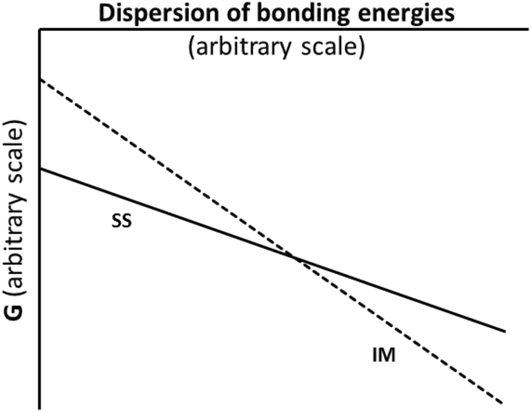
For the sake of simplicity, let us assume that the bonding energies A–A and B–B are identical (H 0), but different than the bonding energy between A and B atoms (H AB). For an equimolar random solid solution, it can be shown that the total enthalpy is (H 0 + H AB)/2. Therefore, if the difference between H AB and H 0 increases (which can be regarded as a larger “scatter”, “dispersion”, or “range” of bonding energies in the alloy), the total enthalpy will vary compared to the enthalpy of pure A or pure B, H 0. This variation is related to half of the dispersion in bonding energies. Besides, in the ordered intermetallic, there are only A–B bonds so that the total enthalpy is H AB. As a consequence, the variation of total enthalpy is related to the difference in bonding energies between H 0 and H AB, not to its half as in the solid solution. Considering only configurational entropy, which is null for the intermetallic, the Gibbs free energy of the intermetallic is equal to its enthalpy. At the opposite, the solid solution possesses a configurational entropy. For a low dispersion in bonding energies between A, B, and AB, e.g., at the extreme if H AB = H 0, the free energy of the intermetallic is H 0 and that of the solid solution is H 0 – T·S conf so that the latter is more stable than the former. When the dispersion in bonding energies increases, both free energies vary, but with a factor two between both, so that there will be a point where the intermetallic becomes more stable than the solid solution. This is illustrated schematically in Fig. 4.
Schematic variation of the Gibbs free energy of a solid solution (SS) and of an intermetallic (IM) when the dispersion in bonding energies increases in an alloy.

Let us now choose two elements A and B so that the dispersion in bonding energies is minimal. The alloy will lie on the left of Fig. 4 and a solid solution will form. Nevertheless, because the dispersion in bonding energies was minimal within the A–B system (it was selected as such), adding a third element C will necessarily increase the scatter in bonding energies: there must be one energy, among H AC and H BC, which differs more from H 0 than does H AB. The alloy A–B–C will therefore lie to the right of the alloy A–B in Fig. 4 (in a ternary system instead of a binary, but the concept still holds). Following this reasoning, adding more and more elements will necessarily result in an increase in the dispersion of bonding energies in the alloy, hence in moving further and further toward the right in Fig. 4 so that there should be a point where an intermetallic will become more stable than the solid solution.
Once again, this model is over-simplistic but it explains why, when increasing the number of elements in an alloy, the enthalpic contribution of intermetallics will always end in overcoming the entropic contribution of the solid solution, and hence why HEAs will become more and more difficult to form. This result is supported by facts: most actual HEAs contain five elements, less are made of six elements, even less contain seven elements, etc. [see also Fig. 1(a)].
C. Thermodynamic point of view
The core principle of the design of HEAs relies on the hypothesis that configurational entropic contribution to the Gibbs energy promotes the stability of disordered solid solutions over other competing phases. This entropic stabilization is represented by the well-known equation of the ideal entropy of mixing when n components are randomly mixed together,  ${}^MS_{\rm{m}}^{{\rm{id}}} = - R\sum\limits_i^n {{x_i}\ln {x_i}}$, which reaches its maximum, R ln n, at equimolarity. However, the above statistical considerations show that mixing five or more principle elements in equal/near equal atomic concentration rarely results in the formation of single disordered solid solutions. In this section, we will point out why the role of configurational entropy in stabilizing solid solutions is overestimated. We will introduce the CALPHAD formalism to express the various contributions to the Gibbs energy of more realistic solid solutions.
1. Thermodynamics of mixtures
We will first restrict ourselves to the case of disordered substitutional solid solutions defined as crystallized phases which can vary in composition and where atoms of different components can occupy the same kind of lattice sites.
In the CALPHAD formalism, the general form of the molar Gibbs energy of such solutions can be expressed as
 $${G_{\rm{m}}} = {}^{{\rm{ref}}}{G_{\rm{m}}} + {}^M{G_{\rm{m}}}\quad ,$$
where refG m accounts for the mechanical mixture of the pure components and MG m represents the thermodynamic effects of mixing:
 $${}^{{\rm{ref}}}{G_{\rm{m}}} = \sum\limits_i {{x_i}{}^0{G_i}\quad ,}$$
 $${}^M{G_{\rm{m}}} = - T \cdot {}^MS_{\rm{m}}^{{\rm{id}}} + {}^E{G_{\rm{m}}}\quad ,$$
where 0G i is the molar Gibbs energy of the elemental constituent i, MG m is the molar Gibbs energy of mixing which describes the behavior of the solution with respect to the reference state, EG m is the excess Gibbs energy which represents the difference between the energies of a real solution and an ideal solution, and  ${}^MS_{\rm{m}}^{{\rm{id}}}$ is the ideal entropy of mixing, also sometimes referred as the configurational entropy.
We now include physical considerations and the underlying statistical thermodynamics of mixtures to discuss more thoroughly the thermodynamic properties of solutions. Let us consider a binary crystal that contains N A = N(1 − x) A atoms and N B = Nx B atoms, with N being the total number of atoms and x being the fraction of B atoms. Assume that these two components are sufficiently alike in atomic size and electronegativity to be interchangeable in a lattice in which each site has z nearest neighbors. The number of possible arrangement of A and B on the lattice is
 $${{N!} \over {\left\{ {N\left( {1 - x} \right)} \right\}!\left\{ {Nx} \right\}!}}\quad .$$
The energy of such a binary crystal depends on the arrangement of atoms and is described by three kinds of bonds, i.e., AA, BB with energies εAA = 20g A/z and εBB = 20g B/z, and AB with energy  ${\varepsilon _{{\rm{AB}}}} = \left( {\nu + {1 \over 2}{\varepsilon _{{\rm{AA}}}} + {1 \over 2}{\varepsilon _{{\rm{BB}}}}} \right)$, where 0g i is the energy of the i constituent (0g i = 0G i/N Av with N Av the Avogadro’s number) and ν is the exchange energy which represents the energy required to change an AA bond and a BB bond into a AB bond. For a particular configuration denoted X, the number of pairs of each kind is
 ${1 \over 2}z\left( {{N_{\rm{A}}} - {\rm X}} \right)$,
 ${1 \over 2}z\left( {{N_{\rm{B}}} - {\rm X}} \right)$, and zX, which gives the configurational energy, E, for this particular configuration:
 $$E = {1 \over 2}z\left( {{N_{\rm{A}}} - X} \right){\varepsilon _{{\rm{AA}}}} + {1 \over 2}z\left( {{N_{\rm{B}}} - X} \right){\varepsilon _{{\rm{AA}}}} + zX{\varepsilon _{{\rm{AB}}}} = {N_{\rm{A}}}{}^0{g_{\rm{A}}} + {N_{\rm{B}}}{}^0{g_{\rm{B}}} + z\nu X\quad .$$
The configurational partition function is
 $$\eqalign{ & \Omega = \sum {{{\rm{e}}^{{{ - E} / {kT}}}}} = \exp \left( {{{ - {N_{\rm{A}}}{}^0{g_{\rm{A}}}} / {kT}}} \right) + \exp \left( {{{ - {N_{\rm{B}}}{}^0{g_{\rm{B}}}} / {kT}}} \right) + \sum {\exp \left( {{{ - z\nu X} / {kT}}} \right)} \cr & = \exp \left( {{{ - {N_{\rm{A}}}{}^0{g_{\rm{A}}}} / {kT}}} \right) + \exp \left( {{{ - {N_{\rm{B}}}{}^0{g_{\rm{B}}}} / {kT}}} \right) + {{N!} \over {{N_{\rm{A}}}!{N_{\rm{B}}}!}}\exp \left( {{{ - z\nu \bar{X}} / {kT}}} \right)\quad , \cr}$$
where the summation extends over all arrangements of atoms on the N lattice sites of the crystal and  $\bar{X}$ is the average value of the various configurations X.
We obtain that the free energy is given by
 $$\eqalign{ & G = - kT\ln \Omega = {N_{\rm{A}}}{}^0{g_{\rm{A}}} + {N_{\rm{B}}}{}^0{g_{\rm{B}}} + kT\ln {{N!} \over {\left\{ {N\left( {1 - x} \right)} \right\}!\left\{ {Nx} \right\}!}} + z\nu \bar{X} \cr & = {N_{\rm{A}}}{}^0{g_{\rm{A}}} + {N_{\rm{B}}}{}^0{g_{\rm{B}}} + NkT\left[ {\left( {1 - x} \right)\ln \left( {1 - x} \right) + x\ln x} \right] + z\nu \bar{X}\quad . \cr}$$
If we assume a completely random mixture where the two components have the same probability of occupying any sites in the crystal lattice (Bragg–William approximation or zeroth approximation), the average value of  $\bar{X}$ is
 $$\bar{X} = {{{N_{\rm{A}}}{N_{\rm{B}}}} \over {{N_{\rm{A}}} + {N_{\rm{B}}}}} = Nx\left( {1 - x} \right)\quad .$$
We then obtain for the molar Gibbs energy of the mixture:
 $${G_{\rm{m}}} = {x_{\rm{A}}}{}^0{G_{\rm{A}}} + {x_{\rm{B}}}{}^0{G_{\rm{B}}} + RT\left[ {{x_{\rm{A}}}\ln {x_{\rm{A}}} + {x_{\rm{B}}}\ln {x_{\rm{B}}}} \right] + {x_{\rm{A}}}{x_{\rm{B}}}L\quad ,$$
where L = zνN Av is the solution parameter, which represents the interactions between the two components.
a. Ideal solutions
We now consider the simplest case of mixture in which constituents mix randomly over the lattice sites with no distinct interactions between them (ν = 0, meaning that εAA = εBB = εAB). In that situation, we can assume that all the possible arrangements of the two atoms have the same configurational energy:
 $$\Omega = \sum {{{\rm{e}}^{{{ - E} / {kT}}}}} = {{N!} \over {{N_{\rm{A}}}!{N_{\rm{B}}}!}}{{\rm{e}}^{{{ - E} / {kT}}}}\quad ,$$
thus the molar Gibbs energy of mixing describing the behavior of the so-called ideal solution is
 $${}^M{G_{\rm{m}}} = RT\left[ {{x_{\rm{A}}}\ln {x_{\rm{A}}} + {x_{\rm{B}}}\ln {x_{\rm{B}}}} \right] = - T{}^MS_{\rm{m}}^{{\rm{id}}}\quad .$$
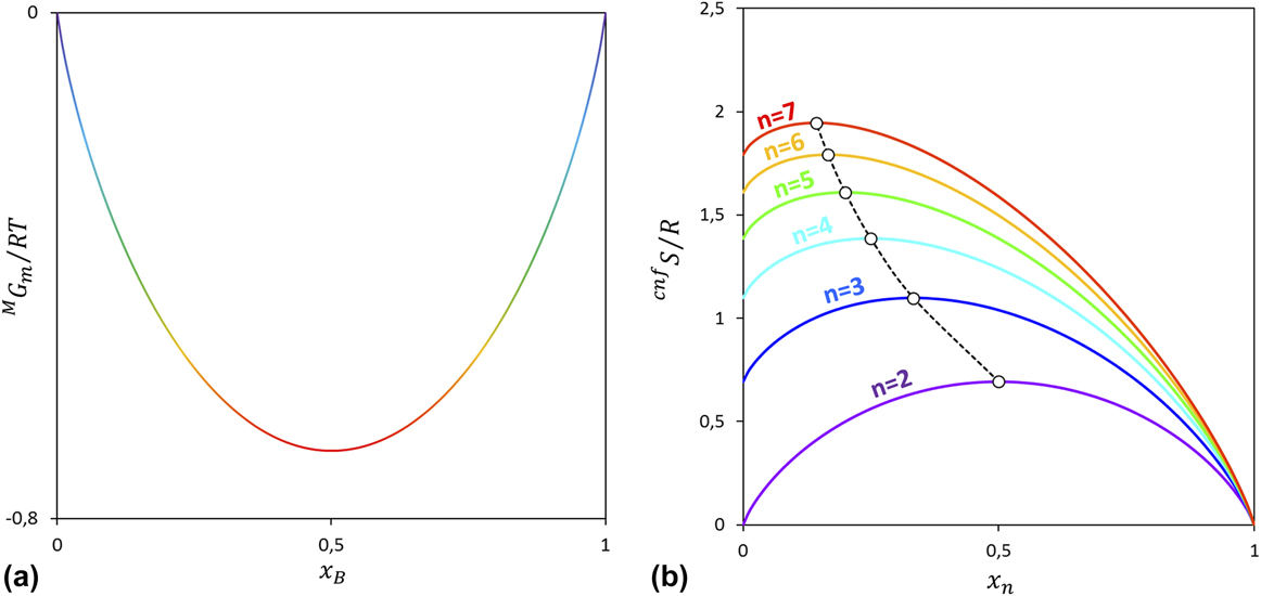
In the case of ideal solutions, the configurational entropy is described by the ideal entropy of mixing. Figure 5(a) gives the calculated Gibbs energy of mixing curve as a function of the composition for a binary ideal substitutional solid solution. The minimum of MG m is achieved when both components have the same fraction. Any deviation from the equimolarity will reduce the number of possible arrangements resulting in a decrease of the configurational entropy. Let us consider what happens when new components (ternary, quaternary, etc.) are mixed. Figure 5(b) shows that the configurational entropy increases with the number of components and that the maximum, cnfS max = R ln(n), is achieved at equimolarity.
(a) Calculated Gibbs energy of mixing for an ideal binary solution and (b) calculated configurational entropy of solid solutions with n components as a function of mole fraction of the nth component.

In principle, incorporating an increasing number of components in equal fractions into a single lattice with random occupancy will promote the stability of a disordered solid solution, presumably over other possible phases, when the configurational entropy dominates the energy landscape. This approach of entropy stabilization of a single-solid solution is the funding principle being explored in multicomponent concentrated alloys, the so-called HEAs. However, the simple formula of the configurational entropy (the ideal entropy of mixing) can apply only to the ideal class of mixtures, i.e., equal energies of the different kinds of bonds and completely random distribution of the different components.
We will now extend the situation to less crude approximation.
b. Regular solutions
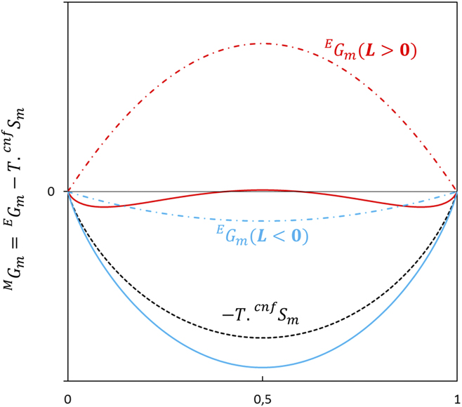
Logically, the next type of mixtures shares the same features describing ideal solutions except that the exchange energy is not zero, i.e., the configurational energy is no longer independent of the arrangement of the components. In this situation, the excess energy of mixing, EG m = x Ax BL, will affect the shape of the Gibbs energy curve which will remain symmetrical with respect to x though, as shown in Fig. 6. A positive value of L (i.e., ν > 0) results in a tendency for demixing in two solid solutions (less A–B bonds than in a random arrangement because A and B do not like to mix with each other). When the temperature decreases, excess energy can counterbalance the configurational entropy. The consequence is that a miscibility gap will form below the critical temperature T sp = x Ax B2L/R at x = 1/2. A negative value of L (i.e., ν < 0) means that unlike atoms prefer to be nearest neighbors (more A–B bonds than in a random arrangement). This will reduce the Gibbs free energy and stabilize the disordered solid solution, as shown in Fig. 6. However, a large negative value of ν will give a tendency of short-range and long-range ordering which will result in deviations from randomness. In this situation, we can no longer consider complete randomness (because the exchange energy influences the number of bonds of different kinds) and the single interaction parameter (regular solution parameter L) is not enough to describe the behavior of real solutions.
Configurational entropy, excess energy of mixing, and resulting Gibbs energy of mixing curves for the sign of the regular solution parameter used.

c. Deviation from random distribution (short-range order)
Neglecting of short-range order (SRO) in the zeroth approximation (the atoms mix randomly) to describe multicomponent mixtures seems questionable. Few theoretical/experimental studies evidenced noticeable SRO in HEAs.Reference Wang, Wang, Lin, Zou, Wu, Hu, Shang, Darling, Wang and Hui30–Reference Widom32 In the CALPHAD approach, a composition dependence of the interaction parameter is then introduced using the Redlich–Kister (RK) polynomial to better fit the experimental data:
 $${}^E{G_{\rm{m}}} = {x_{\rm{A}}}{x_{\rm{B}}}L = {x_{\rm{A}}}{x_{\rm{B}}}\sum\limits_{k = 0}^n {{}^kL{{\left( {{x_{\rm{A}}} - {x_{\rm{B}}}} \right)}^k}} \quad .$$
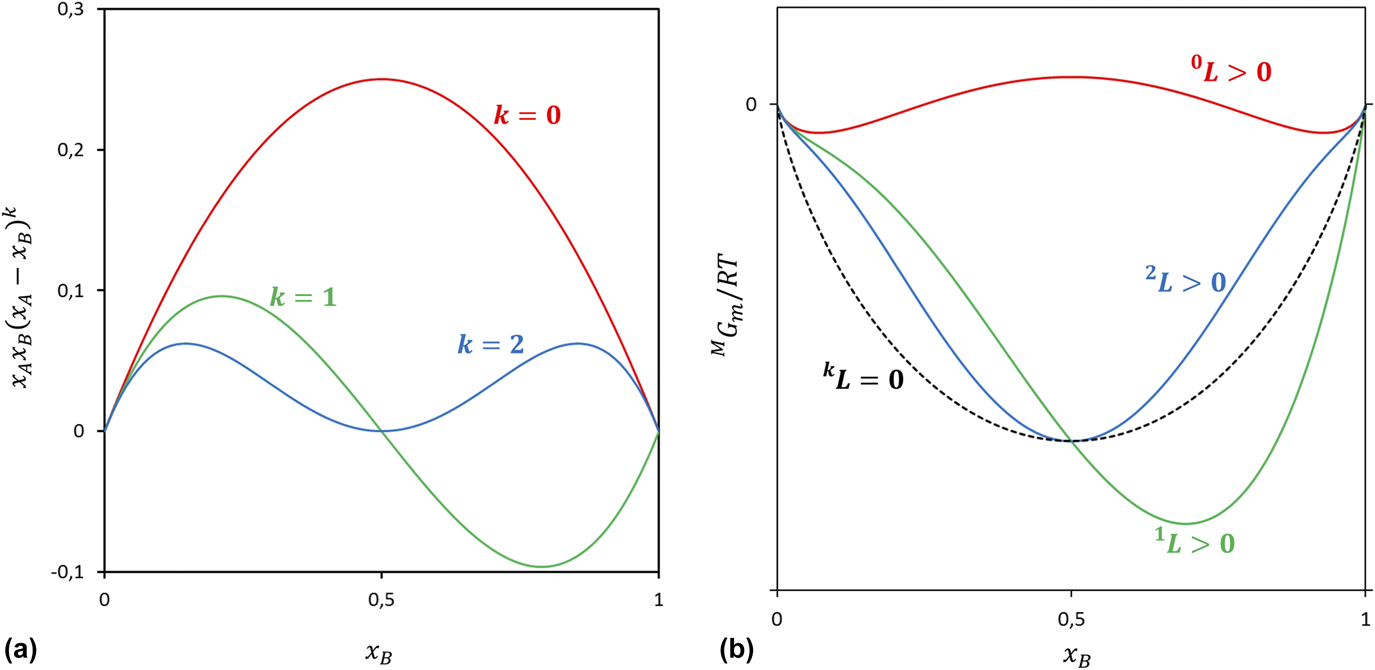
The situation where L is independent of composition corresponds to the regular solution model (k = 0), whereas 1L and 2L are the subregular and subsubregular solution parameters. Figure 7 illustrates the effect of these extra parameters on the shape of the excess Gibbs energy and the Gibbs energy of mixing. In case of a subregular solid solution (k = 1), the Gibbs energy curve is not symmetric and does not reach the minimum at equal amount of components even though equimolarity still provides the highest configurational entropy.
(a) Properties of the RK terms and (b) their effects on the Gibbs energy of mixing.

A temperature dependence of the fitting parameters can be used to introduce the effect of nonideal configurational entropy and nonconfigurational entropy sources:
 $${}^k{L_{{\rm{AB}}}} = {}^k{a_{{\rm{AB}}}} + {}^k{b_{{\rm{AB}}}}T\quad ,$$
ka AB describes the excess enthalpy and kb AB describes the excess entropy.
When SRO occurs, the ideal entropy of mixing does represent only the upper limit of the configurational entropy.
An alternative approach to reproduce the effect of nonrandom distribution solutions is to introduce unlike bond probabilities using the modified compound energy formalism (CEF).Reference Sundman and Ågren33 Higher-order approximations can also be used to model SRO such as the quasi-chemical approachReference Guggenheim34 or the cluster variation methodReference Kikuchi35 in which fictitious constituents are introduced.
d. Long-range order
In the CALPHAD approach, long-range order (LRO) is represented by the use of several sublattices to take into account that atoms of different components can occupy different types of lattice sites. The B2 ordering of the BCC-A2 structure (the atom in the center of the unit cell is different from those at the corners) requires two sublattices with equal amounts of sites (A, B, Va)1(A, B, Va)1 to reproduce antisite fraction and vacancy (Va) defects. The most important ordered phase deriving from the FCC structure is L12 (corner atoms are of a different kind from the atoms on the faces) which can be modeled using two sublattices (A, B, Va)3(A, B, Va)1. More sublattices can be necessary to model ordered phases, intermetallics and metal–nonmetal phases (e.g., M23C6 or to model together L12 and L10), but the number of possible fitting parameters quickly becomes very large. The formalism for describing the Gibbs energy of such phases is the CEF which gives the following expressions:
 $${}^{{\rm{ref}}}{G_{\rm{m}}} = \sum\limits_{{I_0}} {{P_{{I_0}}}\left( Y \right){}^0{G_{{I_0}}}\quad ,}$$
 $${}^{{\rm{cnf}}}{S_{\rm{m}}} = - R\sum\limits_{s = 1}^n {{a_s}} \sum\limits_{i = 1}^{{n_s}} {y_i^{\left( s \right)}\ln \left( {y_i^{\left( s \right)}} \right)\quad ,}$$
 $${}^E{G_{\rm{m}}} = \sum {{P_{{I_1}}}\left( Y \right){L_{{I_1}}}} + \sum {{P_{{I_2}}}\left( Y \right){L_{{I_2}}}} + \cdots \quad ,$$
where I denotes a constituent array on each sublattice s while i denotes an individual constituent, I 0 is the constituent array of zeroth order specifying one constituent in each sublattice,  ${P_{{I_0}}}\left( Y \right)$ is the product of the constituent fractions specified by I 0,
 ${}^0{G_{{I_0}}}$ is the compound–energy parameter representing the Gibbs energy of formation of the compound I 0, a s is the number of sites on each sublattice, and
 $y_i^{\left( s \right)}$ denotes the constituent fraction of i on s.
Additionally, it can be noticed that the entropy is also made of other contributions, e.g., vibrational, electronic, and magnetic entropies, linked to the weight, number of electrons, and magnetic moment of each element and their interactions. As such, it is necessarily composition-dependent, contrarily to the configurational entropy. For instance, first principles calculations have been performed in alloy CoCrFeMnNi, using the density functional theory and finite-temperature ab initio methods.Reference Ma, Grabowski, Körmann, Neugebauer and Raabe36 Simulations considered vibrational, electronic, and magnetic as well as configurational contributions to the entropy. Among others, the results showed that at 1200 K (927 °C), the configurational entropy represents only ∼15% of the total entropy. This may also contribute to explain some of the experimental observations reported above. In CALPHAD formalism, nonideal configurational, vibrational, and electronic contributions are included in the terms EG m and refG m, whereas additional quantities (physG m), modeled separately, can be introduced to account for the contributions arising from physical phenomena which vary sharply with composition such as magnetic transitions. It is not the intention here to describe them.
2. Phase stability
In previous sections, we have examined how entropy and various physical phenomena can alter the Gibbs energy of solutions. However, it is necessary to consider the Gibbs energy of all the competing phases in the determination of phase stability since the equilibrium state is reached at the global minimum of the total energy of the system.
This concept has been reviewed by Zhang et al.Reference Zhang, Zhang, Chen, Zhu, Cao and Kattner37 and Miracle et al.Reference Miracle and Senkov28 to discuss the relative contributions of entropy and enthalpy on phase stability and to emphasize the competition among all the phases of a system. They demonstrated that the lowest energy is not necessarily reached at equimolarity, even though it represents the highest ideal entropy of mixing, and that increasing the number of components promote the formation of secondary phases.
In the following, we will further extend this analysis using hypothetical ternary systems calculated using a user-defined thermodynamic database to feature phase stability with emphasis put on the location of the disordered solid solution in two different situations: when temperature changes and for various combinations of solution parameters.
In the case of ternary systems, the excess Gibbs energy for multicomponent substitutional solution can be written as
 $${}^E{G_{\rm{m}}} = {}^{{\rm{bin}} \cdot E}{G_{\rm{m}}} + {}^{{\rm{tern}} \cdot E}{G_{\rm{m}}}\quad ,$$
With bin·EG m and tern·EG m the binary and ternary excess Gibbs energy contributions:
 $${}^{{\rm{bin}} \cdot E}{G_m} = \sum\limits_{i = 1}^{n - 1} {\sum\limits_{j = i + 1}^n {{x_i}{x_j}{L_{ij}}} } \quad ,$$
 $${}^{{\rm{tern}} \cdot E}{G_{\rm{m}}} = \sum\limits_{i = 1}^{n - 2} {\sum\limits_{j = i + 1}^{n - 1} {\sum\limits_{k = j + 1}^n {{x_i}{x_j}{x_k}{L_{ijk}}} \quad .} }$$
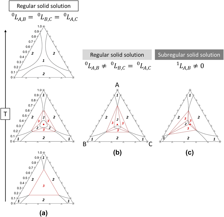
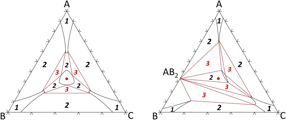
Let us now consider a ternary A–B–C system [Fig. 8(a)] consisting of three binaries forming a regular solid solution with a miscibility gap and having identical solution parameters (0L AB = 0L BC = 0L AC > 0). At low temperature, where the energy landscape is dominated by the excess energy term, the equiatomic composition lies in the middle of the ternary miscibility gap and the solid solution is only stable at the three corners of the phase diagram. When the temperature increases, the solid solution becomes stable for equal amounts of the three components because its Gibbs energy reaches the minimum in the middle of the Gibbs triangle where the configurational entropy is maximum (cnfS m = R ln 3). At higher temperatures, the stability region of the regular solid solution further extends because the contribution of the configurational entropy (−T·cnfS m) overcomes the enthalpy contribution arising from positive binary interactions. The same analysis was performed with further details by Morral and ChenReference Morral and Chen38 for the regular solution model with equal binary interaction parameters only (Meijering’s model). In this discussion, the Gibbs energy surface of the ternary solution was assumed symmetric resulting from identical excess Gibbs energies in all three binaries. This situation is very unlikely, and it is important to point out that contrary to what is observed in binaries, the Gibbs energy surface in a ternary and in higher-order systems will never be symmetric even though the solution behaves like a regular solution. Figure 8(b) shows the consequences of considering a more realistic case where the regular binary solution parameters are different. The stability region of the regular ternary solution deviates from equimolarity. The shift is greater with an increasing gap between the binary solution parameters. The same observation can be made when considering subregular solutions as previously depicted for binary systems [Fig. 8(c)].
Ternary isothermal sections calculated using a hypothetical thermodynamic description of an A–B–C system, highlighting the effect of temperature and binary solution parameters on the stability region of the single disordered solid solution for (a) equal regular solution parameters, (b) different regular solution parameters, and (c) subregular solution parameters. Equimolarity is represented by the red dot. Numbers given are numbers of phases in each phase field.

We now see what happens when one binary intermetallic (AB2 line compound) is introduced in the ternary system. Figure 9 shows that the stable region of the disordered solid solution is not at equimolarity. This is because the contact point between the tangent plane representing the equilibrium and the Gibbs energy surface of the disordered solution  $G_{\rm{m}}^{{\rm{SS}}}$ is not at the minimum point in the middle of the triangle. The tangent plane is tilted to pass through the stable AB2 intermetallic, leading to a shift of the tangent point on
 $G_{\rm{m}}^{{\rm{SS}}}$ toward A–C richer compositions.
Ternary isothermal sections calculated using a hypothetical thermodynamic description of an A–B–C system, highlighting the effect of LRO (intermetallic AB2) on the stability region of the single disordered solid solution. Equimolarity is represented by the red dot. Numbers given are numbers of phases in each phase field.

In summary, these simple thermodynamic calculations of hypothetical ternary diagrams illustrate that equimolarity does not represent the minimum energy of nonideal solutions and that phase stability results from a competition between phases driven by the minimization of the total Gibbs energy. Incorporating more than two components in a mixture increases the configurational entropy but shifts the minimum of the Gibbs energy away from equimolarity in the case of nonideal solutions and can lead to the formation of a more stable compound. For example, it was observed that the stability temperature range of a single solid solution in nonequimolar alloy Co20Cr15Fe26Mn17Ni22 was larger than that of equimolar alloy CoCrFeMnNi,Reference Mroz25 confirming that maximum solid solution stability does not occur at equimolarity. The same concept is supported by the formation of a single solid solution in nonequimolar alloy Al2.8CoCrCuFeNi whereas equimolar alloy AlCoCrCuFeNi does not form any.Reference Yeh, Chen, Lin, Gan, Chin and Shun10
We can conclude that a truly entropy-stabilized single solution is an improbable event very occasionally encountered around equimolarity for near-ideal solid solutions only. This conclusion is supported by the work of Otto et al.Reference Otto, Yang, Bei and George39 who have analyzed the microstructure and thermodynamic properties of five quinary alloys by replacing individual elements in the so-called Cantor’s alloy (i.e., CoCrFeMnNi). They evidenced that the FCC solid solution made of ten binary pairs of Cantor’s alloy behaves closely as an ideal solid solution, which results in the formation of a true solid solution alloy, whereas all substitutional alloys exhibited multiphase microstructures. On the theoretical front, Schön et al.Reference Schön, Duong, Wang and Arroyave40 recently probed the different contributions to phase stability in multicomponent systems. Their work provides strong evidence that entropy has a marginal effect in stabilizing concentrated disordered solid solutions when SRO exists and that conflicting interactions and correlations (what they called configurational frustration) drive the stabilization of the disordered phase in the central region of the composition space.
III. CALPHAD AS A RETROSPECTIVE COMPUTATIONAL APPROACH TO EXPLAIN EXPERIMENTAL RESULTS
A. Few successful examples of CALPHAD used to explain experimental observations (microstructure development in HEAs)
Several resources cited below outline the utilization of computational thermodynamics and CALPHAD databases to explain the microstructure development in HEAs and CCAs. The main value of these predictive thermodynamic approaches is to gain a better understanding of the effect of given elements on phase stability and more generally on the relationships between composition, processing, and microstructure. These practices can be categorized into two broad kinds: calculations under equilibrium and nonequilibrium conditions, respectively.
1. Calculation and inspection of phase diagrams
The microstructure of an alloy results in the competition among all the possible phases in the studied system. Phase diagrams map the phase stability regions as a function of temperature, pressure, and alloy concentration. They are useful for guiding the development of new alloys because they provide the phase field of operation and detailed information on the equilibrium state, including phases present, their volume fractions, compositions, and transformation temperatures. Still only few studies highlight the application of the CALPHAD approach to analyze the microstructure of HEAs under annealed (equilibrium) conditions and to compare model calculations and experimental observations.Reference Zhang, Zhang, Chen and Cao41–Reference Liu, Gao, Liaw and Zhang44 They were already thoroughly reviewed by Gao et al.Reference Gao, Yeh, Liaw and Zhang45
In this section, we illustrate the CALPHAD approach through an example, by analyzing the formation of the single fcc solid solution in the Cantor’s alloy from the thermodynamic properties of the Co–Cr–Fe–Mn–Ni quinary system. Zhang et al.Reference Zhang, Zhang, Chen, Zhu, Cao and Kattner37 used binary phase diagrams to discuss the mutual solubility of the components in this system. In the present paper, we expand the analysis to ternary and quaternary phase diagrams and introduce parallel coordinate plots to visualize the compositional relationship among the components in the fcc structure and delimitate the range of the single fcc phase. The calculations below were performed by interfacing Matlab® and ThermoCalc® software and the TCHEA2 database. In this database, all ten binaries and half of the ten ternaries were assessed in the full range of composition and temperature (Co–Cr–Fe, Co–Cr–Ni, Co–Fe–Ni, and Cr–Fe–Ni) or partially assessed (Fe–Mn–Ni). The five remaining ternaries are extrapolated from their respective constitutive binaries which may lead to inaccurate representations of the Gibbs energy for the phases in these systems. It should be noted that higher-order systems are absent in the CALPHAD database so that the contributions from quaternary and quinary interactions on the Gibbs energy model are neglected.
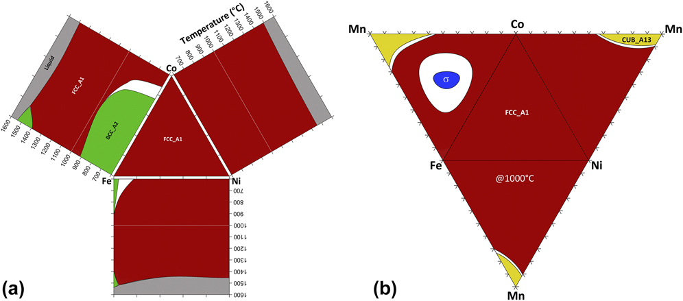
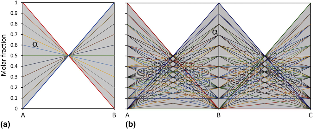
Figure 10(a) shows the isothermal section at 1000 °C of the Co–Fe–Ni system and the three subcomponent binary systems. Co, Fe, and Ni possess the fcc structure at 1000 °C, are mutually soluble in the fcc structure, and consequently form a continuous fcc solid solution in this ternary at 1000 °C. Adding Mn which does not have the same crystal structure leads to the formation of the σ phase in the Co–Fe–Mn ternary [Fig. 10(b)]. This phase admits Ni in solid solution, so σ can extend in the quaternary Co–Fe–Mn–Ni and limit the range of the single fcc solid solution. Visual examination of the quaternary to identify the composition range where the fcc phase is stable can be performed using a 3D plot of the fcc surface boundary. An alternative approach to visualize n-dimensional data is the parallel coordinate system that maps multidimensional data into a 2D space without losing information. In a parallel coordinate plot, the axes for the variables run vertically and span from the minimum to maximum value of each variable. Figure 11 illustrates the construction principle of such plot using simple cases. Consider the range of existence of a solid solution α in binary system A–B at constant temperature [Fig. 11(a)]. The two variables X A and X B (representing the molar fractions of A and B) lie parallel to each other. Capturing the relationships between these variables is done by representing segmented lines connecting the corresponding values of X A and X B for which the α phase exists at the considered temperature. Now assume mutual solubility between A and B (i.e., continuous solid solution α over the full composition range at the fixed temperature), then segmented lines connect all the possible values of the composition parameters from 0 to 1 with the constraint that X A + X B = 1. The value X A = 1 is connected to X B = 0, and so on every fixed increments down to X A = 0 and X B = 1. This gives an envelope representing the range of existence of the solid solution α [Fig. 11(a)]. Figure 11(b) extends the same representation to a hypothetical ternary A–B–C.
(a) Calculated subcomponent binaries and isothermal section at 1000 °C of the ternary phase diagram of the Co–Fe–Ni system. (b) Unfolded tetrahedron of the quaternary Co–Fe–Ni–Mn system showing the isothermal section of the 4 subcomponent ternaries calculated at 1000 °C.

Hypothetical A–B (a) binary and A–B–C (b) ternary systems illustrating the construction principle of the parallel coordinate plot in the case of the continuous solid solution α.

Applying the same construction principles to the stability range at 1000 °C for the main phases (fcc, bcc, hcp, and σ) in the quinary Co–Cr–Fe–Mn–Ni system gives the linear mapping shown in Fig. 12(a). The problem with representing a 2D answer to a multidimensional problem is that it is too static. The parallel coordinate plot is meant to be dynamic/interactive and gives different results for different questions. To make such plot readable, we have reduced the essential information with respect to the range of existence of the fcc solid solution. This is done in Figs. 12(b)–12(d) for the Co–Fe–Ni, Co–Fe–Ni–Mn, and Co–Fe–Ni–Mn–Cr systems at 1000 °C. The continuous fcc solid solution in the Co–Fe–Ni ternary is reflected by the fact that lines connect all the possible values of the component concentrations [Fig. 12(b)]. The same data set (861 composition calculations) is displayed by a scattergram of the Co–Fe–Ni system [the inset of Fig. 12(b)] that shows the absence of clustering, meaning that the fcc phase expands over the entire ternary composition space at this temperature. Figure 12(c) shows what happens when adding Mn (12,341 composition calculations). The fcc single-phase is still stable over a large range of composition in the Co–Cr–Fe–Mn system. Up to 90% of Mn can be dissolved in the fcc structure. Cr tends to have a stronger effect on the stability of the fcc single-phase, as illustrated in Fig. 12(d) (135,751 composition calculations). A maximum 45 at.% of Cr can be dissolved in fcc only when the solid solution is depleted in Fe and Mn, as highlighted by the red lines connecting the 45 and 42.5 at.% Cr compositions to the other coordinates representing the molar fractions of Co, Fe, Ni, and Mn in the fcc phase.
2D parallel coordinate plots showing the compositional relationship in the stability range of the fcc, bcc, hcp, and σ phases at 1000 °C in the quinary Co–Fe–Ni–Mn–Cr system (a). The composition relationships delimiting the range of existence of the stable phases is represented by lines connecting the component concentrations in five parallel vertical axes with a 2.5 at.% compositional increment. The range of existence of the fcc single-phase solid solution at 1000 °C is shown in (b) for Co–Fe–Ni, (c) for Co–Fe–Ni–Mn, and (d) for Co–Fe–Ni–Mn–Cr systems. The insert is a scattergram showing the existence of the fcc single solid solution in the Co–Fe composition space of the Co–Fe–Ni system (the size of the dots is proportional to the Ni content).

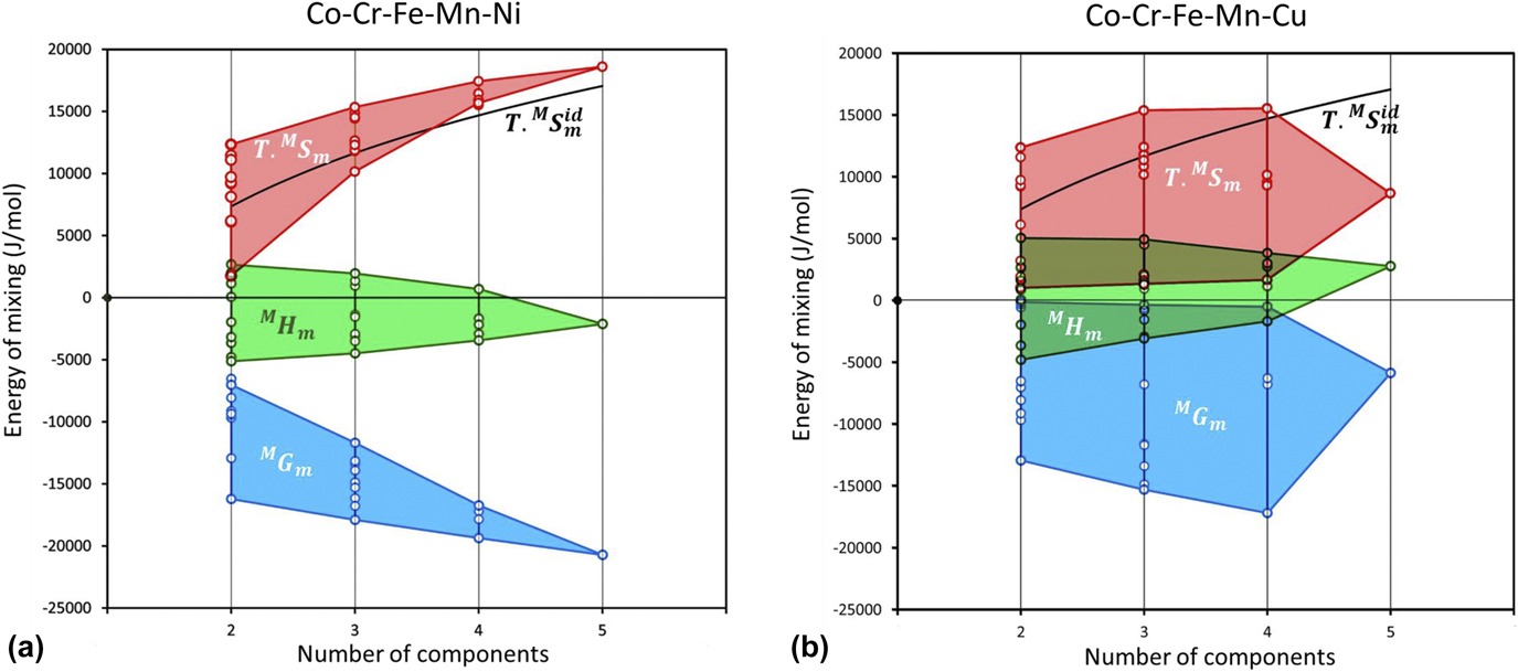
CALPHAD allows us to examine the underlying thermodynamic properties of mixtures. Figure 13 compares the calculated energies of mixing (Gibbs energy, enthalpy, and entropy) in the fcc disordered phase. Comparisons between the Co–Cr–Fe–Mn–Ni and Co–Cr–Fe–Mn–Cu quinary systems shed light on the ability of the Cantor’s alloy to form a model HEA (single disordered solid solution at equimolarity). Replacing Ni by Cu in the quinary alloy changes the relative importance of the enthalpy and entropy contributions. Compared to the Ni-quinary, the Cu-quinary has less entropy. In contrast with the Ni-quinary, the increase in dimensionality from 4 to 5 results in a decrease of the entropy of mixing. This behavior arises from the demixing tendency due to the pair interactions with Cu. All the binary excess enthalpies with Cu (Co–Cu, Cr–Cu, Fe–Cu, Mn–Cu) are positive which results in a positive enthalpy of mixing in the Cu-quinary while it is negative in the Ni-quinary. Both enthalpy and entropy effects lead to the destabilization of the fcc disordered solution when replacing Ni by Cu. These results show that the trend observed in the concentrated region of multicomponent systems can be derived from the properties of the constitutive binary systems if the solution behaves as an ideal or near-ideal mixture (for instance, the Ni–Cu solid solution is exploited in “Monel” or cupronickel alloys, and the formation of copper-rich solid solution clusters is used in some precipitation-hardened steels). This is the case for the Cantor’s alloy which can be regarded as a model HEA. When Ni is replaced by Cu in the concentrated quinary, the mixture deviates from ideality. In this case, increasing the number of components does not lead to an increase in the entropy, and enthalpy contributions have a large effect in destabilizing the fcc solid solution.
Calculated energies of mixing (Gibbs energy, enthalpy, and entropy) of the fcc disordered phase at 1000 °C in the Co–Cr–Fe–Mn–Ni (a) and Co–Cr–Fe–Mn–Cu (b) quinary systems and their subcomponents (each point represents the interactions in the ten binaries, ten ternaries, and five quaternaries).

2. Nonequilibrium calculations—modeling solidification
Although the formation of a single solid solution at equilibrium is a requirement to form a HEA, the microstructure of an alloy is dictated not only by composition but also by processing. To determine the resulting microstructure for a given processing route, the equilibrium phase diagrams are generally insufficient, and phase transformations must be modeled to quantitatively describe the kinetics of formation and evolution of the microstructure. The first step in alloy processing is casting so that solidification and the resulting microstructures are of prime importance.
In an attempt to explain the as-cast microstructure of HEAs, including the type and amount of phases and the compositional microsegregation, thermodynamic simulations of the solidification process can be performed based on the CALPHAD approach. Two basic models are commonly used to simulate the solidification paths: equilibrium lever rule and nonequilibrium Scheil–Gulliver.Reference Scheil46,Reference Gulliver47 The first condition assumes global equilibrium between liquid and solid phases, infinite diffusion in both phases, and no undercooling during nucleation or growth, while the latter condition stipulates thermodynamic equilibrium at the liquid–solid interface, infinite diffusion in liquid, and no diffusion in solid, so the liquid composition is homogeneous whereas the solid phases will retain the successive compositions from when they have been formed on cooling. The Scheil–Gulliver model has been applied successfully to some practical cases for 3d transition metal CCAs and refractory metal CCAsReference Zhang, Zhang, Chen and Cao41,Reference Zhang, Gao, Zhang, Yang and Guo48,Reference Zhang, Gao, Zhang and Guo49 owing to the sluggish diffusion in these systems and the fast cooling rates resulting from the arc-melting technique generally used to produce them. However, erroneous estimations of the solidification path and significant discrepancies between simulations and experiments are often observed. They can have a thermodynamic origin, i.e., unprecise thermodynamic description reduces the reliability of the calculations, and can also arise from the assumption from the Scheil model where diffusion in the solid is neglected.
Real solidification paths range between the two above limiting cases, and certain components may redistribute within already solidified phases through diffusion. Thus, kinetic simulations are needed to give more accurate description of the mass and heat fluxes in the solidification process. In the absence of available diffusion data, different scenarios for back-diffusion can be tested to evaluate the effect of fast diffusing elements with the hope to improve the predicted solidification.
B. Limitations of CALPHAD—unsuccessful examples
In the CALPHAD technique, Gibbs energy models with parameters describing each phase in a multicomponent system are obtained based on experimental and first principles information for the constituent binary and ternary systems and then are extrapolated to higher-order systems once thermodynamic descriptions for the relevant lower order systems are known:
 $$G_{\rm{m}}^\varphi = \sum\limits_i {{x_i}{}^0G_i^\varphi - T \cdot {}^MS_{\rm{m}}^{{\rm{id}}}} + {}^{{\rm{bin}} \cdot E}G_{\rm{m}}^\varphi + {}^{{\rm{tern}} \cdot E}G_{\rm{m}}^\varphi \quad .$$
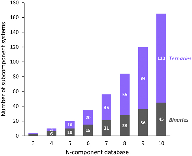
The Gibbs free energy parameters are stored in thermodynamic databases for various applications, such as calculations of phase diagrams by determining the minimum global energy in the composition space. CALPHAD databases are generally developed for a particular alloy family, so they contain a limited number of elements and the full thermodynamic assessment of the Gibbs energies is usually given only for compositions enriched with one main element which depends on the database. Nonetheless, the amount of available data, collected over tens of years, is such that quite precise assessments could be performed in the case of classical alloys, leading to a rather good predictive performance. By contrast, by definition, HEAs/CCAs lie in the central regions of multidimensional phase diagrams, well outside the bounds usually used to construct databases and optimize the energy model parameters. As a consequence, the HEA field, being recent, could not benefit from a long history of data collection and model assessment and is confronted to the nature and vastness of covered compositional ranges. Calculations in these vast composition spaces require large extrapolations from the classical thermodynamic models which may lead to inaccurate evaluations of the Gibbs energies and phase equilibria. Reliability and accuracy of the predictions can thus become questionable when obtained from incomplete thermodynamic descriptions. Nevertheless, efforts are taken to develop databases for multiconcentrated alloys, but (i) some of them are limited to small numbers of elements, i.e., they specialize on certain families of alloys (e.g., Al Co–Cr–Fe–Ni,Reference Zhang, Zhang, Chen and Cao41 Co–Cr–Fe–Mn–Ni,Reference Haase, Tang, Wilms, Weisheit and Hallstedt50 Co–Cr–Cu–Fe–Mn, and Cr–Nb–Ti–V–Zr),Reference Zhang, Zhang, Chen, Zhu, Cao and Kattner37 the database PanHEA from CompuTherm® contains only ten elements and (ii) some are limited to a small number of phases,Reference Raghavan, Hari Kumar and Murty51 although larger databases dedicated to HEAs start appearing by coupling experiment to first principles calculations (ThermoCalc® – TCHEA2). To perform accurate predictions, databases should contain large numbers of binary and ternary phase diagrams, if possible assessed on full compositional ranges. Figure 14 shows the number of subcomponent thermodynamic descriptions (binaries and ternaries) required to describe higher-order systems. Available commercial databases remain far from these numbers, and while some of them provide full thermodynamic descriptions of all binary systems, only few ternaries are available in the full range of composition and temperature even for the recent databases developed for HEAs. For example, the TCHEA database developed by ThermoCalc® contains 185/190 fully assessed binary systems and 135/1140 fully assessed ternaries for twenty elements. Caution should be placed on the reliability of predictions when the system description includes unassessed lower order systems since it is unclear how uncertainties propagate to higher-order systems. Senkov et al.Reference Senkov, Miller, Miracle and Woodward52,Reference Senkov, Miller, Miracle and Woodward53 defined a credibility criteria for CALPHAD calculations based on the fraction of fully thermodynamically assessed binary systems (F AB) and the fraction of fully assessed ternary systems (F AT) included in the database. These theoretical credibility criteria provide a weighting scheme to evaluate the reliability of predictions from extrapolations of multicomponent systems. More confidence can be placed on CALPHAD calculations performed using databases with high F AB and F AT for a given system.
Number of binary and ternary thermodynamic descriptions required for complete thermodynamic database descriptions as a function of the number of elements.

Another concern existing with CALPHAD databases is that quaternary and higher-order interactions are rarely (probably never) evaluated. The rational is that these terms may have negligible influence on the Gibbs energy. This might be true for dilute mixture; however the results of Schön et al.Reference Schön, Duong, Wang and Arroyave40 suggest that due to the complex interactions and synergy between components (SRO parameters), the thermodynamics of concentrated multicomponent solid solutions cannot be deduced from the behavior of the subcomponent binary systems. The absence of quaternary and higher-order interactions in the current thermodynamic descriptions may have an impact as evidence is provided for the existence of SRO.
Until recently, though, most studies would involve the use of general-purpose databases like SSOL or of databases developed for other categories of alloys, e.g., for steels or nickel alloys, and no large-scale assessment has been made of the performance of databases specialized in HEAs. A few examples have been described previously but, in this respect, a large-scale assessment has been recently conductedReference Tancret, Toda-Caraballo, Menou and Rivera-Díaz-Del-Castillo54 using a published database of several hundreds of real multiconcentrated alloys, including several tens of HEAs.Reference Toda-Caraballo and Rivera-Díaz-del-Castillo27 The actual formation—or not—of a single solid solution was compared to predictions made with ThermoCalc® software using four commercially available databases: SSOL5, TCFE8, and TCNI7 as well as TTNI8 (at the time of study, the TCHEA1 thermodynamic database was only a subset of the TCNI database, and it later evolved toward TCHEA2 by taking into account some specific features of HEAs). Calculation details are described in the original paper,Reference Tancret, Toda-Caraballo, Menou and Rivera-Díaz-Del-Castillo54 and results are summarized in Fig. 15.
Success (dark sectors) and failure (light sectors) in predicting the formation of HEAs and non-HEAs, using TCNI7, TTNI8, TCFE8, or SSOL5 database, on several tens or hundreds of actual multiconcentrated alloys, depending on cases.

Still, this result is rather optimistic for at least two reasons:
(i) When “success” is announced for the prediction of an actual HEA, it does not mean that the predicted and experimental stability temperature ranges agree, nor even that they overlap at all; it means that a single solid solution was experimentally obtained at least at one temperature and that a single solid solution was predicted at least at one temperature, but not necessarily at the same temperature.
(ii) When “success” is announced for the prediction of an actual non-HEA, it does not mean that the predicted and experimental phases are the same; it just means that no single solid solution could be obtained experimentally and that the alloy was not predicted single-phase at any temperature (irrespective of the nature, amount, and range of existence of phases).
The actual fractions of “success” should therefore be even lower than appearing in Fig. 15.
The main conclusion was that no database could be fully trusted in predicting phase formation in multiconcentrated alloys since it appears that there are cases where CALPHAD succeeds in predicting phase formation in multiconcentrated alloys and other cases where it fails. Developments are still needed and are made toward a better performance (e.g., with the TCHEA2 database), in the hope that CALPHAD can become an efficient tool for HEA design, as it has become for other categories of alloys. In a recent paper, Gao et al.Reference Gao, Zhang, Gao, Zhang, Ouyang, Widom and Hawk55 reviewed and discussed the barriers for developing reliable thermodynamic databases and the solutions to overcome them utilizing the methodologies of empirical thermophysical parameters, CALPHAD method, and first principles calculations combined with hybrid Monte Carlo/molecular dynamics simulations. In the meantime, predicted trends nevertheless give valuable information, and CALPHAD has indeed been used at least as a guide for HEA design, sometimes in conjunction with other tools as exposed hereafter.
IV. THERMODYNAMICS AS PREDICTIVE TOOLS FOR HEA DESIGN
A. Rules and models for HEA design
1. Classical methods for HEA design
In fact, the mostly used methods to explain the formation of a single solid solution in multiconcentrated alloys do not rely on CALPHAD. Indeed, most authors make use of rather classical approaches, based on a number of physicochemical parameters and rules. They are worth being mentioned here since they can be seen as concurrent to CALPHAD or, as will be explained later, as complementary tools.
For instance, some of the classical Hume-Rothery rules for the solubility of metalsReference Hume-Rothery56 have been adapted or extended to HEAs:
(i) The pure metals must have the same crystal structure. If this is a requirement for complete solubility, it is not one for HEAs: there are cases of multiconcentrated solid solutions of metals with different crystal structures before alloying. For example, AlCoCrCu0.5Ni forms a single BCC phaseReference Yeh, Lin, Chin, Gan, Chen, Shun, Tsau and Chou57 although only Cr has a BCC structure as a pure metal: Co is either hexagonal or FCC, and the others are FCC. Consequently, this rule does not apply to HEAs.
(ii) Elements must have similar sizes. This rule has been applied to multiconcentrated alloys, by calculating the average atomic size mismatch, δ.Reference Zhang, Zhou, Lin, Chen and Liaw17,Reference Fang, Xiao, Xia, Li and Dong58 It was found that most HEAs were associated with small values of δ and that high values of δ would not allow the formation of a single solid solution.
(iii) To achieve complete solubility, the valence of atoms must be similar, which brings a criterion on the alloy electron concentration. Two criteria are based on this rule; on the one hand, the average number of itinerant electrons per atom, e/a, and on the other hand, the valence electron concentration, VEC. Both have been applied to multiconcentrated alloys.Reference Poletti and Battezzati59–Reference Guo, Ng, Lu and Liu61
(iv) Atoms must have comparable electronegativities, χ, since elements with different electron affinities tend to form stronger bonds and hence favor ordered intermetallics compared to disordered solid solutions. This brought the definition of the average electronegativity mismatch, Δχ, which has been used in multiconcentrated alloys.Reference Fang, Xiao, Xia, Li and Dong58,Reference Guo, Ng, Lu and Liu61
Other criteria have also been suggested to predict the formation of solid solutions, based on thermodynamic concepts (but not using the CALPHAD approach):
(v) Because it makes part of the total Gibbs energy, the enthalpy of mixing, ΔH mix, calculated by a summation of interactions between pairs of elements,Reference Miedema, de Châtel and de Boer62 has been proposed as a criterion for the formation of HEAs.Reference Zhang, Zhou, Lin, Chen and Liaw17
(vi) To take into account the balance between enthalpy and entropy in the stability of a phase, the parameter Ω was proposed, defined as the product of melting temperature and mixing entropy, divided by the absolute value of the mixing enthalpy.Reference Yang and Zhang63
(vii) Finally, considering that phase separation from a solid solution could occur by spinodal decomposition, it has been proposed that a large gap between the spinodal decomposition temperature and the melting temperature would guarantee the formation of a single solid solution at high temperature. This yielded the parameter µ, defined as the ratio between the melting temperature and the critical spinodal decomposition temperature.Reference Poletti and Battezzati59
However, a careful analysis of experimental results gained on several hundreds of multiconcentrated alloysReference Toda-Caraballo and Rivera-Díaz-del-Castillo27 showed that none of the above-mentioned parameters, taken alone, could separate strictly HEAs from non-HEAs. In fact, most non-HEAs would lie within certain parametric ranges while most HEAs would fall within other ranges, but the latter would also cover many non-HEAs, and vice versa. Also, it was shown that “two-dimensional maps” of different couples of parameters allow us to identify regions in which many HEAs lie. Nevertheless, it was still observed that such regions containing many HEAs also cover many non-HEAs, and reciprocally. As a consequence, these criteria, taken alone or by pairs, may be seen as necessary conditions for the obtention of HEAs, but not as sufficient conditions, so that they cannot be used for alloy design. Actually, this is confirmed by the fact that although such parametric approaches have often been announced as potential tools for HEA design, it seems that the number of actual HEAs that have been designed by explicitly using them is very limited. One can find, for instance: Hf0.5Nb0.5Ta0.5Ti1.5Zr,Reference Sheikh, Shafeie, Hu, Ahlström, Persson, Veselý, Zýka, Klement and Guo64 HfNb0.5TiV0.5Zr, HfNb2TiVZr2, HfMo0.5Nb0.5TiZr, and HfNb0.5Ta0.5TiZr.Reference Chen, Li, Cheng, Wu, Cheng and Xu65
2. CALPHAD for HEA design
Besides, since it provides fair estimates of phase formation in alloys, including in multiconcentrated ones, CALPHAD has logically been used to design new HEAs, although this seems not to have been the most common practice in the discovery of the majority of existing HEAs to date. Nevertheless, successful examples exist. In general, authors report that they pre-identified a short list of elements, based on physicochemical rules (see. Sec. IV.A.1) or considering existing binary and/or ternary phase diagrams to check for maximum solubilities of elements by pairs or triplets, or by starting with already known HEAs and modifying their composition in a limited manner. Then CALPHAD calculations are used to spot the domains of single-phase stability, to confirm presumptions and/or to refine composition. This is usually made by calculating single equilibria, pseudo-binary, or pseudo-ternary phase diagrams around given systems. Sometimes the approach fails as the predictive capacity of CALPHAD is not perfect as already stated, but several new HEAs have been successfully designed using such methods, e.g., Co20Cr15Fe26Mn17Ni22,Reference Mroz25,Reference Fraczkiewicz66 CrxMoNbTaVW,Reference Zhang, Gao, Zhang and Guo49 MoNbTaTiVW,Reference Zhang, Gao, Zhang, Yang and Guo48 MoNbTaTiV,Reference Yao, Qiao, Hawk, Zhou, Chen and Gao67 CoCuFeMnNi, CoFeMnNiV, AlFeMnNbTi, AlCrFeMnV and CoCrFeMnV,Reference Tazuddin, Gurao and Biswas68 Co10Cr15Fe40Ni25V10, Co10Cr15Fe25Mn10Ni30V10, Co10Cr10Fe25Mn12Ni33V10, Cr15Fe22Mn13Ni40V10, and Cr10Fe30Mn20Ni30V10.Reference Choi, Jung, Jo, Lee and Lee69
3. Beyond thermodynamics: data mining
It was previously shown that both simple physicochemical criteria (e.g., Hume-Rothery derived rules) and CALPHAD would fail in a number of occasions to predict the occurrence of a single solid solution in multiconcentrated alloys or to predict when several phases will form, which is problematic in an alloy design perspective.
Another way that was used, either independently of these methods or coupled to them, is data mining. The latter is here understood in the general meaning of extracting knowledge from data using purely mathematical or statistical tools.
As already stated, physicochemical parameters (δ, e/a, VEC, Δχ, ΔH mix, Ω, or µ), considered alone, cannot be used for alloy design. It is not possible either using pairs of such parameters, although using two-parameter maps can increase the predictive efficiency, which was tested on more than 320 highly concentrated multicomponent alloys.Reference Toda-Caraballo and Rivera-Díaz-del-Castillo27 This trend was confirmed by Asensio Dominguez et al. through a principal component analysis of data with up to five physical parameters (ΔH mix, ΔS mix, δ, Δχ, and VEC), over a set of 79 alloys, showing that increasing the number of parameters being taken into account simultaneously would provide an improved predictive efficiency.Reference Domínguez, Goodall and Todd70 They used their approach to design successfully two four-element single-phase equimolar alloys, MnFeCoNi and TiVMnNb. Besides, Nong et al.Reference Nong, Zhu, Cao, Yang, Lai and Liu71 used an artificial neural network to successfully predict what solid solution phase would form in a HEA, from four of the physical parameters previously mentioned (δ, ΔH mix, Δχ, and VEC). However, the approach could not predict if a single phase would form in any multiconcentrated alloy or not since only single-phase HEAs were included in the database. The method was proposed, but not actually used, for HEA design. Also, based on an analysis of 109 equimolar or multiconcentrated alloys, it was suggested that combining computational thermodynamics with some physical parameters would bring extra information,Reference Raghavan, Hari Kumar and Murty72 although this proposal was not used to design new alloys. Finally, Tancret et al. performed a thorough analysis of a database of more than 320 multiconcentrated alloys, by coupling a Gaussian process statistical analysis over nine calculated physicochemical parameters (including δ, e/a, VEC, Δχ, ΔH mix, Ω, and µ) to CALPHAD—using simultaneously four thermodynamic databases as exposed earlier.Reference Tancret, Toda-Caraballo, Menou and Rivera-Díaz-Del-Castillo54 Of course, using a single thermodynamic database optimized for HEAs would probably have given better predictions than several less appropriate ones, but at the time of study, no such ThermoCalc database would exist for HEAs. Nevertheless, it was shown, on pragmatic grounds through a comparison with experimental results on actual alloys, that such a combination of tools could eliminate the risk not to form a single solid solution in highly concentrated multicomponent alloys, although none of the tools or parameters could achieve it if taken separately. This was used to propose 62 new potential equimolar HEAs, although there was no experimental validation. The use of such an approach for the design of actual alloys will be detailed later.
B. Systematic exploration of phase diagrams and compositional systems
In the past decade, the development of HEAs and CCAs mainly relied on a trial-and-error approach where most of the alloys are engineered by starting with a mixture of four or five principal elements, and adding a solute element that leads to the enhancement of certain mechanical properties, typically strength and ductility, and continuing to add that element until the best compromise is obtained. This often occurs with little knowledge of the microstructure and the related phase fields of operation.
Recently, computational thermodynamics and various CALPHAD databases were used to obtain multicomponent phase diagrams allowing to better understand the effect of given elements on phase stability and more generally on the microstructure. To illustrate the value of these thermodynamic approaches, we have presented in Sec. III.A few successful examples of equilibrium and nonequilibrium calculations performed to analyze the microstructures in HEAs and CCAs.
In spite of the theoretical and pragmatic limitations previously exposed, the CALPHAD technique and dedicated databases for multicomponent systems have remarkably developed so that the ability of CALPHAD to anticipate the phases present, their volume fractions and transformation temperatures, or at least the trends it gives, can be utilized to develop a quantitative computational design approach of HEAs and CCAs. Such predictive approaches in which CALPHAD is used to target the alloy compositions that are the most capable of producing the ideal microstructure for achieving the desired properties are still limited. Following this principle, Gao et al.Reference Gao, Carney, Dogan, Jablonksi, Hawk and Alman73 have explored phase stability in sixteen multicomponent systems to identify HEAs (single-phase alloys) in the bcc structure. They also applied the same strategy to propose new HEAs in hcp and fcc structures.Reference Gao, Yeh, Liaw and Zhang45,Reference Gao and Alman74 A more general effort encompassing the phase stability of 130,000 equimolar alloy systems was undertaken by Miracle et al.Reference Miracle, Miller, Senkov, Woodward, Uchic and Tiley75 and Senkov et al.Reference Senkov, Miller, Miracle and Woodward52,Reference Senkov, Miller, Miracle and Woodward53 They developed a strategy based on high throughput computation to identify the most promising HEA candidates among a pallet of 45 elements for structural applications. Their approach rely on a systematic exploration of the phase diagrams of each alloy calculated using CALPHAD and simple rules to evaluate alloy’s potential for structural applications based on present phases, transformation temperatures, and rough estimates of their microstructure-insensitive properties.
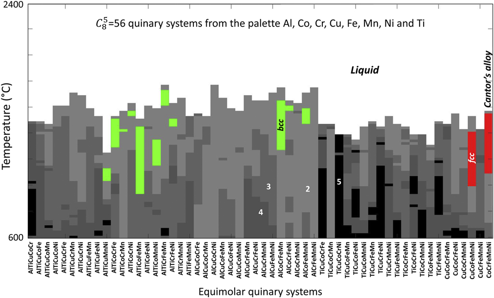
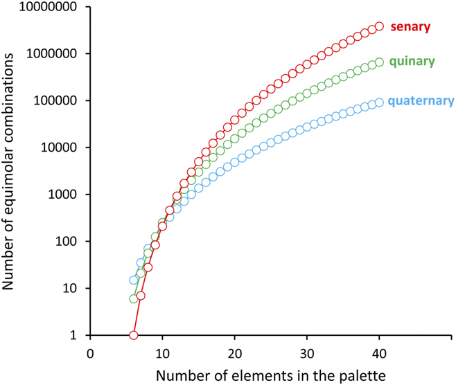
As an additional illustration of such approaches, Fig. 16 shows the systematic exploration of the phase stability space achieved by mapping the composition and temperature dependence of equilibrium states. In this example, the phase stability map for all possible equimolar quinary combinations (a total of 56, see Fig. 17) from a pallet of ten elements was constructed using a CALPHAD thermodynamic database (TCHEA2) and a Matlab algorithm interfaced with ThermoCalc. Mapping here displays the regions of existence of single-phase solid solutions (bcc and fcc) and of multiphase constitutions. Such a map can conveniently be used to browse, search, and visualize specific phase stability states (e.g., the thermodynamic conditions for the stability of a single-phase solid solution) as a function of composition and temperature. A general comment can be made at this point: single-phase domains, corresponding to HEAs, are much less present than multiphase domains, corresponding to CCAs. This could already be anticipated by looking at proportions of HEAs and non-HEAs among existing multiconcentrated alloys [Fig. 1(a)], or by considering the solely statistical chances of forming a single solid solution in a multicomponent alloy (Fig. 2). This opens a vastness in potentially interesting CCAs that exceeds by far that of HEAs.
Calculated phase stability maps for all possible equimolar quinary alloys from a palette of ten elements as a function of temperature. Red and green regions highlight the single-phase fields for the fcc and bcc solid solutions, respectively. Gray scale is a function of the number of phases in equilibrium.

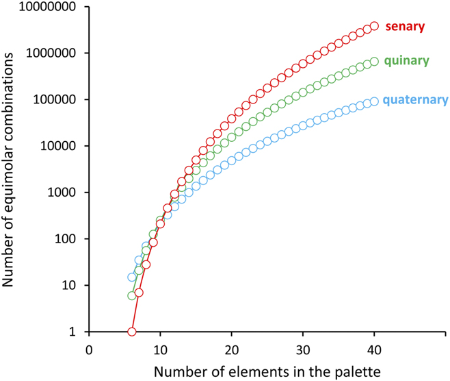
Number of equimolar quaternary, quinary, and senary alloys as a function of the number of elements in the palette.
Computational thermodynamics aided multiconcentrated alloy design approaches must face a challenge regarding the vastness of the multidimensional composition space to be explored. This immensity of the design space was stressed in a recent review,Reference Miracle and Senkov28 stating that “the materials community is now thrust into an uncharted, hyperdimensional territory that is […] difficult to explore […]. The vastness is frightening”. For instance, in a system made of sixteen elements as recently investigated,Reference Tancret, Toda-Caraballo, Menou and Rivera-Díaz-Del-Castillo54 it may exist more than ten thousand billion nonequimolar alloys containing between five and eight elements, with a step of 1% between 5 and 35%. Calculating a single equilibrium by CALPHAD takes, on a modern computer core, between a few tens of milliseconds and several seconds depending on the complexity of the calculation to be made so that the total calculation time could reach (virtually) tens or even hundreds of thousands of years at least!
C. Guided/intelligent exploration of the compositional space
As shown above, a naive systematic exploration of a given design space is not compatible with up-to-date computing capabilities. Of course, decreasing the number of elements considered and/or increasing the concentration and/or the temperature steps would drastically reduce the computing time, but making it reasonable would severely degrade the alloy design ambitions. Intensive parallel computing is also a way forward but using billions of computing cores simultaneously is out of reach at present. To circumvent this combinatorial and computational problem, several other strategies have been proposed recently. For instance, a modest but systematic calculation of all possible equimolar alloys (1287), with a list of thirteen elements, was performed with the combined physicochemical and data mining approach exposed in Sec. IV.A.Reference Tancret, Toda-Caraballo, Menou and Rivera-Díaz-Del-Castillo54 This led to the identification of 62 potential HEAs that were then evaluated by CALPHAD by four different thermodynamic databases: they were all predicted to be single phased for at least one temperature by at least one database. Although illustrative, this approach is “guided” because a fast computing tool (mining of data based on physicochemical parameters) is first used in a preselection step, followed by a more computer-intensive CALPHAD evaluation. Such an approach could potentially be extended to much larger sets of alloys, e.g., including more elements and/or for nonequimolar compositions. Indeed, screening millions or billions of different materials could be possible with a data mining tool and/or using simple physicochemical parameters. This was illustrated recently by the systematic calculation of some physicochemical parameters for nearly 200 million equimolar alloys within a 73-element system, leading to less than 2000 potential HEAs.Reference King, Middleburgh, McGregor and Cortie76 Then, it should be possible to use CALPHAD to calculate only hundreds or thousands of pre-identified alloys, or even hundreds or thousands if necessary, which is within computational reach.
Still, such systematic methods are not adapted to explore the immensity of the design space mentioned earlier. More recently, metaheuristic approaches, i.e., optimization techniques, have been implemented to explore the design space in a guided/“intelligent” manner, by progressively converging toward potentially interesting regions of the design space only. This was illustrated, for instance, by the optimization of the strength of HEAs in the Al–Cr–Co–Fe–Ni system using molecular dynamics simulations and a cuckoo search optimization technique,Reference Sharma, Singh, Liaw and Balasubramanian77 although no experimental validation was made. A CALPHAD counterpart of such an approach has also been proposed to explore the Co–Cr–Fe–Mn–Ni system using a constraint-satisfaction algorithm,Reference Abu-Odeh, Galvan, Kirk, Mao, Chen, Mason, Malak and Arroyave78 to identify potentially interesting nonequimolar compositions, although there was no experimental validation. In fact, the design space was not as large as previously exposed, and it would be possible to explore it systematically by choosing appropriate steps: with five elements between 15 and 25% as reported, if a step of 1% is chosen for each element, this makes less than 10,000 alloys; with 100 temperature levels this would require 1 million CALPHAD equilibria, which should be calculable in a reasonable time (e.g., days or weeks). Nevertheless, the search method would be worth being applied to much larger systems. Such a use of a search algorithm has recently been applied to the design of new FCC HEAs within a multi-objective optimization scheme.Reference Menou, Toda-Caraballo, Rivera-Díaz-del-Castillo, Pineau, Bertrand, Ramstein and Tancret79 A genetic algorithm was used to simultaneously maximize the chances to produce a single phase (based on a data mining criterion already presentedReference Tancret, Toda-Caraballo, Menou and Rivera-Díaz-Del-Castillo54), maximize solid solution hardening as evaluated by a physical modelReference Toda-Caraballo and Rivera-Díaz-del-Castillo80 and minimize the density estimated by a rule of mixtures. The search was undertaken over a huge design space of sixteen elements (Al–Co–Cr–Fe–Mn–Mo–Nb–Ni–Ta–Ti–V–W–Zr–Cu–Hf–Ru) with contents from 5 to 35% for each element by steps of 1%. CALPHAD was then used a posteriori to assess phase formation in 846 Pareto-optimal alloys identified by the search algorithm. An alloy was selected (Al10Co17Fe34Mo5Ni34), fabricated, thermomechanically processed, and tested. It displays a single and ductile FCC phase and a superior combination of mechanical properties and density than other large-grain and annealed FCC HEAs. By combining physicochemical criteria as well as physical models, data mining, CALPHAD, and a multi-objective optimization algorithm, and leading to the successful experimental validation of a new HEA with improved properties, this work represents to date the most advanced integrated HEA design strategy involving CALPHAD.
D. Goal-oriented search—the role of CALPHAD in the key development strategies of the CCAs’ next generation
Until recently, the main motivation of the HEA community was to find new equiatomic or near–equiatomic combinations of elements to promote the formation of fcc, bcc, or hcp single-phase-disordered solid solutions. Although solid solution hardening is an important strengthening mechanism, it is not the most efficient and a single solid solution microstructure may not be the ideal one for many applications. For example, high strength is better achieved in alloys containing a distribution of one or more kinds of precipitates to inhibit dislocation motion. Inspired by the successes achieved in aluminum alloys, steels, and nickel superalloys, multiphase microstructures are now becoming a key approach toward the development of CCAs with better balance of strength and ductility.Reference Miracle13,Reference Gorsse, Miracle and Senkov26,Reference Miracle and Senkov28,Reference Li, Pradeep, Deng, Raabe and Tasan81,Reference He, Wang, Huang, Xu, Chen, Wu, Liu, Nieh, An and Lu82 So, it should be possible to adapt optimization strategies to the design of CCAs, by using CALPHAD to search for specific constitutions that are likely to bring high mechanical properties, i.e., combinations of phases, for instance mixtures of an fcc solid solution with L12 intermetallics as in nickel-based superalloys, of a bcc solid solution with B2 intermetallics, of several solid solutions as in some bronzes or titanium alloys, of solid solutions with carbides or nitrides as in many steels, etc. It should be stressed that the microstructure of an alloy is dictated by both its chemistry (alloy composition) and the way it has been processed (thermomechanical treatments), so alloy design requires an advanced understanding of the relationships between processing, microstructure, and properties (the metallurgical paradigm) to determine the conditions which can deliver the ideal microstructure to improve performance. To determine the resulting microstructure for a given thermomechanical processing route, the equilibrium phase diagrams are generally insufficient, and phase transformations must be modeled to quantitatively describe the kinetics of formation and evolution of the microstructure to help understand the changes during given thermomechanical treatments or solidification. In the following, we present two examples that illustrate how CALPHAD can be used to guide the design of two well-known microstructure templates found in age-hardenable Ni alloys and austenitic twinning-induced plasticity (TWIP) or transformation-induced plasticity (TRIP) steels.
1. CALPHAD aided design of precipitation-strengthened CCAs
Precipitation is a phenomenon that can occur in an alloy when the matrix phase is supersaturated with respect to one or more solute elements. It involves the nucleation, growth, and coarsening of one or more secondary phases. These processes depend on both thermodynamic (driving forces) and kinetic parameters (diffusivities of the solutes). They can be captured with simple continuum models similar to that developed by Deschamps and BréchetReference Deschamps and Brechet83 for the treatment of precipitation in Al and Mg alloys.Reference Hutchinson, Nie and Gorsse84 The nucleation and growth of each phase is described within the framework of classical nucleation theoryReference Aaronson, Lee and Aaronson85,Reference Russell86 and diffusional growth theory.Reference Zener87 The nucleation is written as
 $${{{\rm{d}}N} \over {{\rm{d}}T}} \cong {N_0}Z\beta \exp \left( {{{ - \Delta {G^*}} \over {kT}}} \right)\quad ,$$
where N 0 is the number of nucleation sites per unit volume, Z is the Zeldovich’s factor, and β is the frequency factor that describes the attachment kinetics of atoms to the nucleus. The most important parameter entering this equation is the activation barrier for nucleus formation, ΔG*. For spherical precipitates, the nucleation barrier can be expressed as
 $$\Delta {G^ * } = {{16} \over 3}\pi {{{\gamma ^3}} \over {{{\left( {{{\Delta {G_{\rm{m}}}} / {{V_{\rm{m}}}}}} \right)}^2}}}\quad ,$$
where γ is the interfacial energy separating the nucleus and the matrix, ΔG m is the onset chemical driving force for nucleation, and V m is the molar volume of the precipitate phase. The thermodynamic quantity DGm, necessary for calculations of precipitation kinetics, can be obtained from the Gibbs energies of the involved phases when their thermodynamic description is available, as illustrated in Fig. 18.
Schematic molar Gibbs energy diagram with the curves for the α and ε phases in a binary system A–B. The tangent construction to calculate the onset driving force ΔG m for precipitation of ε from a metastable supersaturated α matrix is illustrated.

An example of analysis which can be conducted to explain the microstructure development in CCAs is shown in Fig. 19 for the Al0.3CoCrFeNi alloy.Reference Bouaziz, Allain, Scott, Cugy and Barbier88 In this alloy, a fine γ′-L12 precipitate distribution is developed in the γ-fcc matrix during annealing although the equilibrium phase field of operation consists of fcc + B2 + σ. The onset driving forces for nucleation, calculated using ThermoCalc coupled to a user-defined code with Matlab and the TCHEA2 thermodynamic database, highlight the competition of the different phases. As shown in Fig. 19, the nucleation of the L12 phase is favored over the other competing equilibrium phases. This suggests that even though the L12 phase does not have the highest onset driving force, it precipitates first due to the low γ/γ′ interfacial energy, hence to a lower energy barrier for nucleation.
Normalized nucleation barriers for homogenous precipitation of L12, B2, bcc, and σ phases from the supersaturated fcc solid solution with Al0.3CoCrFeNi composition.

2. CALPHAD-aided design of TWIP HEAs
An exceptional balance of strength and ductility can be achieved in materials exhibiting high work-hardening capability. This results from the activation of mechanical twinning or ε or α′ martensitic transformations (in steels) induced by straining, which are competitive to dislocation glide during deformation.Reference Bouaziz, Allain, Scott, Cugy and Barbier88 This led to the concepts of TWIP and TRIP. The competition between these mechanisms is largely controlled by the magnitude of the stacking fault energy (SFE). Twinning is reported to occur at SFE between 18 and 45 mJ/m2,Reference Allain, Chateau and Bouaziz89 while dislocation glide is activated at SFE above 45 mJ/m2 and martensite formation below 16 mJ/m2. In other words, an alloy with a low SFE is more likely to deform by twinning or by a strain-induced martensitic transformation. To select one of these deformation mechanisms, the magnitude of the SFE has to be finely tuned to the appropriate range by adjusting the chemistry of the alloy. This approach is subject to intense research activity in the steel community since the discovery of high manganese TWIP steels in 1888.Reference Hadfield90 In these steels, low SFE and the segregation of C to the dislocations is responsible for mechanical twinning which acts as obstacles to dislocation glide.Reference Rémy91 Otto et al.Reference Otto, Dlouhy, Somsen, Bei, Eggeler and George92 and Gludovatz et al.Reference Gludovatz, Hohenwarter, Catoor, Chang, George and Ritchie93 were among the first to report the occurrence of deformation-induced twinning in the Cantor’s alloy to explain the exceptional fracture toughness at cryogenic temperatures. These studies opened up the way to new routes for the development of TWIP fcc HEAs by empirical designReference Li, Pradeep, Deng, Raabe and Tasan81,Reference Deng, Tasan, Pradeep, Springer, Kostka and Raabe94 or by ab initio calculations to predict the SFE.Reference Beyramali Kivy and Asle Zaee95 The above-mentioned empirical approach was also successfully used to propose new TRIP CCAs.Reference Li, Pradeep, Deng, Raabe and Tasan81 The strategy is based on the modification of the SFE by changing the chemical composition to obtain the activation of different deformation mechanisms and promote either nanotwinning or a strain-induced martensitic transformation at room temperature.
The magnitude of SFE, γSFE, of γ-austenite (fcc solid solution) can be estimated on a thermodynamic basis, as a function of the temperature and solute content, which offers the mean to explore the effect of alloy components on the SFE. The example we provide below to illustrate this idea uses the model developed by Olson and CohenReference Olson and Cohen96 in which the SFE represents the Gibbs energy required for the formation of two atomic layers of ε-martensite within the dense planes:
 $${\gamma _{{\rm{SFE}}}} = 2\rho \Delta {G^{\gamma \to \varepsilon }} + 2{\sigma ^{{\gamma / \varepsilon }}}\quad ,$$
where ρ is the surface density of atoms in the {111} planes, ΔG γ→ε is the change in the molar Gibbs energy upon phase transformation γfcc → εhcp, and σγ/ε is the surface energy of the interface γ/ε.
The difference of the molar Gibbs energy ΔG γ→ε between γ and ε martensite formation can be calculated from the Gibbs energy descriptions of the γ and ε phases from the TCHEA CALPHAD databases. Figure 20 shows an attempt to correlate the magnitude of SFE to the chemical composition. The relative influence of the level of concentration of each alloying element is predicted with respect to the Al0.3CoCrFeNi composition. Al and Ni are shown to increase the SFE, while Co, Cr, and Fe decrease the SFE. Al has the greatest effect. Keeping in mind the lack of accuracy of current thermodynamic databases and that low SFE is a necessary but not sufficient condition for the activation of mechanical twinning, SFE predictions using CALPHAD can be regarded as a useful design guidance to select alloying elements and adjust their composition to exploit TWIP effect in HEAs or CCAs. However, the previous approaches to develop TWIP and/or TRIP HEAs used empirical conceptsReference Li, Pradeep, Deng, Raabe and Tasan81 or ab initio simulations.Reference Beyramali Kivy and Asle Zaee95 Due to their empirical nature or to the long time that is needed to run simulations, none of these approaches would be suited to an efficient computational alloy design strategy to optimize alloy properties, neither by a systematic screening of a reduced compositional space, nor by a guided/intelligent exploration as described earlier. At the opposite and as already demonstrated, CALPHAD makes fast predictions and can be advantageously used as a computational design tool. In this respect, this opens the way for multi-objective optimization of HEAs and CCAs where the SFE is an explicit criterion, among others like phase constitution, solid solution hardening, precipitation hardening, density, cost, etc., with vast perspectives in terms of potential properties.
Predicted effect of each element on the variation of the SFE with respect to the Al0.3CoCrFeNi alloy at 300 K. Each line represents the change due to the variation in composition of one given element while the others remain constant. For Co, alloy composition varies from Al0.3Co0.7CrFeNi to Al0.3Co1.3CrFeNi. The same range is applied for Cr, Fe, and Ni, while with Al, the composition spans from Al0Co0.7CrFeNi to Al0.3Co0.7CrFeNi.

V. CONCLUSION
This review article has summarized and discussed the recent development of computational thermodynamics (e.g., CALPHAD) for the study and development of HEAs and CCAs.
The concept of entropy-stabilized single solid solution in multiprincipal element alloys was critically tested based on statistical analysis of both experimental observations and simple combinatorial principles, as well as thermodynamic considerations regarding the role of entropy on the Gibbs energy and phase stability. It was shown that the probability of forming a single solid solution decreases with an increase in the number of alloying elements and favors the formation of intermetallics. Using the CALPHAD formalism and hypothetical thermodynamic descriptions, we have investigated the effect of configurational entropy in stabilizing solid solutions. Our results prove that incorporating more than two components in a mixture shifts the minimum of the Gibbs energy away from equimolarity in the case of nonideal solutions and can lead to the formation of a more stable compound. It is also shown that the stabilizing effect of entropy is presumably often overestimated except for ideal mixtures. Our investigations lead us to the conclusion that a truly entropy-stabilized single solution is an improbable event very occasionally encountered around equimolarity for near-ideal solid solutions only (for which Cantor alloy can be regarded as emblematic).
Examining the uses of CALPHAD in the field of HEAs and CCAs, we have outlined two different practices: (i) as a retrospective approach to explain observations related to the microstructure development as a function of the alloy composition and processing conditions under both equilibrium and nonequilibrium situations and (ii) as a predictive design tool to explore the composition space and identify the most promising candidates capable of producing the ideal microstructure for achieving the desired properties. This critical review of the state-of-the-art, along with original results, shows that CALPHAD is an efficient tool that gives valuable information and guidelines for the study and the design of HEAs and CCAs. We stressed that computational thermodynamics aided design must face two challenges that arise from the very nature of multiprincipal element alloys. The first challenge concerns the need for more accurate descriptions of the Gibbs energy curves in the central region of the multidimensional composition space. Great effort should be put into the description of subcomponent ternary systems within the full compositional ranges to improve the reliability of the predictions. The second challenge results from the immensity of the design space to be explored which can make the application of systematic approaches inappropriate due to the computing time needed to explore the space of possibilities. Alternative, more efficient, approaches to dramatically accelerate the discovery of new materials can rely on the integration of CALPHAD with other design tools, such as physicochemical criteria, data mining, and optimization techniques, to guide the computational exploration to the most promising portions of the design space with higher chances of finding optimal solutions.
Finally, we have highlighted the role of CALPHAD to guide the design of three well-known microstructure templates, respectively, found in age-hardenable Ni alloys and austenitic TWIP or TRIP steels, which represent key development strategies for the next generation of HEAs and CCAs. The first approach relies on the calculation of nucleation barrier maps for the design of precipitation-strengthened CCAs. The second example concerns the compositional mapping of the SFE to exploit TWIP and/or TRIP effects in HEAs or CCAs.