



1. Introduction
Falling bodies in fluid, from drifting autumn leaves to coins dropped in water, have long fascinated scientists. Their trajectories and stability arise from fluid–structure interaction (FSI), where inertial, viscous and elastic forces (when present) compete to dictate motion. A classic example is the descent of a plate-like body in air: by perturbing the surrounding fluid, it creates a pressure difference between its upper and lower surfaces, generating lift that sustains a passive flight state. Passive flight is widely observed in nature, with plant seeds using rotation or oscillation to slow descent and extend dispersal distances, and spiders using flexible silk threads to migrate in the wind. Understanding the mechanisms behind passive flight is crucial for both fundamental fluid mechanics and biomimetic design, such as micro-air vehicles.
Theoretical studies of falling plates date back to Maxwell (Reference Maxwell1852), who identified the critical role of the relative locations of the centre of gravity and centre of pressure. Subsequent research, such as the landmark experiments by Willmarth et al. (Reference Willmarth, Hawk and Harvey1964), mapped the flight modes in terms of Reynolds number
 $ \textit{Re}$
and dimensionless moment of inertia
 $ I^*$
, showing that heavier bodies tend to tumble, while lighter ones flutter. More recent studies have refined this picture, demonstrating that transitions between these states can be chaotic and governed by a low-dimensional dynamics (Field et al. Reference Field, Klaus, Moore and Nori1997; Andersen et al. Reference Andersen, Pesavento and Wang2005). While much attention has been given to rigid bodies, introducing structural flexibility fundamentally enriches the problem. Alben (Reference Alben2010) demonstrated that flexibility can alter the flight state of a falling sheet, with experiments by Tam (Reference Tam2015) showing that flexible wings can enhance lift and prolong flight by storing and releasing elastic energy. Lau & Huang (Reference Lau and Huang2021) further explored how varying flexibility in a viscous fluid yields distinct descent patterns, establishing flexibility as a key control parameter for passive flight.
A particularly interesting case is the ‘winged seeds’ of plants, such as those in the Dipterocarpaceae family. Unlike uniform sheets, these seeds feature a heavy, concentrated mass at the centre or leading edge, supported by a lightweight, flexible wing. Rabault et al. (Reference Rabault, Fauli and Carlson2019) demonstrated that the curvature and mass distribution of such seeds are optimised for slow descent, while Vincent et al. (Reference Vincent, Zheng, Costello and Kanso2020) showed that non-uniform flexibility in a tumbling wing can improve flight efficiency by reducing drag. Despite these advances, the specific interaction between a concentrated weight and a flexible membrane remains underexplored in the context of passive flight.
The wake of a falling body, or the pattern of vortices it sheds, is closely linked to its descent dynamics. For example, a heavy disk or sphere descending almost vertically typically produces a classic Kármán vortex street (2S shedding pattern, i.e. two single vortices per cycle). When conditions change, the wake can transition to a 2P mode (two pairs of vortices per cycle), typically coinciding with larger-amplitude planar oscillations of the body. Previous studies (Mathai et al. Reference Mathai, Zhu, Sun and Lohse2017) showed that the transition from 2S to 2P shedding in falling bodies is governed by factors like the mass ratio and moment of inertia. Understanding this interplay between vortex shedding and motion is key to explaining the transitions between fluttering, tumbling or spiralling behaviours.
Most previous studies on falling plates have considered either rigid bodies with prescribed geometry and mass distribution, or flexible sheets and plates whose weight and inertia are distributed over the entire body. In these systems, mode selection is usually discussed in terms of Reynolds number, moment of inertia and overall flexibility. The centrally weighted flexible plate considered here is mechanically different: the gravitational driving force is localised at the centre, whereas the elastic restoring force and hydrodynamic loading are distributed along the deformable plate. This separation between localised forcing and distributed deformation creates a distinct FSI problem, relevant to lightweight flexible wings or winged-seed-like structures carrying a compact mass. It also gives rise to falling regimes that are absent or not emphasised in previous uniformly weighted flexible-plate studies, including the swing and stable falling modes.
Motivated by this physical distinction, we systematically perform numerical simulations of the free fall of a flexible plate driven by a concentrated central weight in both two-dimensional (2-D) and three-dimensional (3-D) scenarios. We map the flight dynamics and identify four distinct descent modes: swing, stable falling, fluttering and tumbling. To capture the underlying physics, we introduce the effective stiffness
 $ \textit{Kg} = K / G$
, which quantifies the competition between bending stiffness and concentrated gravitational loading, and use it to accurately organise the mode transitions and collapse the kinematic data. Additionally, we explore a bistability phenomenon at the fluttering–tumbling transition dependent on the initial inclination angle, and investigate vortex-shedding transitions within the swing mode. In 3-D simulations, we examine finite-span effects and reveal new flight behaviours, such as spanwise oscillations in wide plates. These findings offer new insights into the passive flight of non-uniformly weighted structures, with potential applications in micro-air vehicles and the dispersal of plant seeds.
The paper is organised as follows: the physical problem and mathematical formulation are described in § 2, the numerical method and verification are detailed in § 3, the results are discussed in § 4 and concluding remarks are provided in § 5.
 $(a)$
Schematic illustration of a 2-D flexible plate falling under a concentrated weight
 $ G_c$
. Two instants are shown: at
 $ T = t_0$
, the plate remains undeformed with the initial inclination angle
 $ \theta _0$
; at
 $ T = t_1$
, the plate bends as it descends, representing a typical instantaneous falling configuration.
 $(b{-}e)$
Representative falling modes observed in simulations:
 $(b)$
swing,
 $(c)$
stable falling,
 $(d)$
fluttering and
 $(e)$
tumbling.

Figure 1. Long description
A schematic illustration of a two-dimensional flexible plate falling under a concentrated weight. Two instants are shown: at T equals t 0, the plate remains undeformed with the initial inclination angle theta 0. At T equals t 1, the plate bends as it descends, representing a typical instantaneous falling configuration. The diagram includes labels for the plate length (L), the concentrated weight (G_c), the end-to-end distance (D) of the deformed plate, and the initial inclination angle. The x and y axes are also indicated. Representative falling modes observed in simulations are depicted in separate panels: Panel A shows a straight plate at the initial time, Panel B shows a fluttering mode in red, Panel C shows a stable falling mode in blue, and Panel D shows a tumbling mode in green. Panel E illustrates a chaotic falling pattern.
Schematic of the 3-D flexible plate:
 $(a)$
initial configuration and
 $(b)$
a snapshot during descent. Here,
 $ L$
and
 $ W$
denote the chord length and span width, respectively, and
 $A_r=W/L$
is the aspect ratio. The concentrated weight
 $G_c$
is uniformly distributed along the nodes indicated by the red line. The initial inclination angle is
 $\theta _0$
.

2. Physical problem and mathematical formulations
As illustrated in figure 1
 $ (a)$
, we consider the sedimentation of a 2-D flexible plate of length
 $L$
in an initially quiescent fluid, driven solely by a weight
 $G_c =m_c g$
concentrated at the centre of the plate, where
 $m_c$
is the concentrated mass and
 $g$
is the magnitude of gravitational acceleration
 $\boldsymbol{g}$
. In the 3-D cases, we consider plates with different span widths
 $W$
. The concentrated weight
 $G_c$
is uniformly distributed along the spanwise centreline of the plate, corresponding to the row of mid-chord nodes indicated by the red line in figure 2. The gravitational force acting on the rest of the plate is neglected. This configuration abstracts practical FSI systems where a lightweight flexible membrane or wing carries a heavily localised payload, such as winged seeds (e.g. samara) during passive dispersal or micro-air vehicles with a central mass. To rigorously justify the validity of neglecting the distributed self-weight of the lightweight plate, a comprehensive sensitivity analysis is provided in Appendix A, which confirms that its inclusion yields negligible quantitative corrections to the macroscopic kinematics and mode transitions. The governing equations for the flow are the Navier–Stokes equations
 \begin{align} \frac {\partial \boldsymbol{v}}{\partial t}+\boldsymbol{v} \boldsymbol{\cdot }\boldsymbol{\nabla }\boldsymbol{v}=-\frac {1}{\rho } \boldsymbol{\nabla }p+\frac {\mu }{\rho }{\nabla} ^2 \boldsymbol{v}+\boldsymbol{f}, \\[-28pt] \nonumber \end{align}
 \begin{align} \boldsymbol{\nabla }\boldsymbol{\cdot }\boldsymbol{v}=0, \\[0pt] \nonumber \end{align}
where
 $\rho$
is the fluid density,
 $\boldsymbol{v}$
is the velocity,
 $p$
is the pressure,
 $\mu$
is the dynamic viscosity and
 $\boldsymbol{f}$
represents the body force exerted by the immersed boundary on the surrounding fluid.
The Euler–Bernoulli beam equation is adopted to resolve the deformation and kinematics of the flexible plate
 \begin{align} \rho _s h \frac {\partial ^2 \boldsymbol{X}}{\partial t^2} & =\sum _{i, j=1}^2 \frac {\partial }{\partial s_i}\left \{\varphi _{\textit{ij}}\left [\delta _{\textit{ij}}-\left (\frac {\partial \boldsymbol{X}}{\partial s_i} \boldsymbol{\cdot }\frac {\partial \boldsymbol{X}}{\partial s_{\kern-1pt j}}\right )^{-1 / 2}\right ] \frac {\partial \boldsymbol{X}}{\partial s_{\kern-1pt j}}-\frac {\partial }{\partial s_{\kern-1pt j}}\left (\gamma _{\textit{ij}} \frac {\partial ^2 \boldsymbol{X}}{\partial s_i \partial s_{\kern-1pt j}}\right )\right \} \nonumber \\ & \quad +\boldsymbol{F}_{\kern-1pt s}+\boldsymbol{F}_{\kern-1pt c}+\boldsymbol{F}_{\kern-1pt g}, \end{align}
where
 $ \boldsymbol{X}(s_1, s_2, t) = (X, Y, Z)$
denotes the position vector of the plate, where
 $s_1$
and
 $s_2$
are the Lagrangian coordinates in the chordwise and spanwise directions, respectively. The density and thickness of the plate are given by
 $\rho _s$
and
 $h$
. The term
 $\boldsymbol{F}_{\kern-1pt s}$
represents the Lagrangian force exerted by the surrounding fluid,
 $ \boldsymbol{F}_{\kern-1pt c}$
is the repulsive force to avoid contact and overlap between plate elements and
 $ \boldsymbol{F}_{\kern-1pt g} = G_c \boldsymbol{g}/g$
is the weight added at the centre of the plate. The in-plane stiffness tensor is defined as
 $\varphi _{\textit{ij}}$
, with
 $\varphi _{11}=\varphi _{22}= \varphi$
being the stretching stiffness and
 $\varphi _{12}= \xi$
the shearing stiffness. The bending stiffness is characterised by the out-of-plane effect matrix
 $\gamma _{\textit{ij}}$
, where
 $\gamma _{11}= \gamma$
. Here,
 $ \delta _{\textit{ij}}$
represents the Kronecker delta. The boundary conditions at all edges are
 \begin{align} \varphi _{\textit{ij}}\left [\delta _{\textit{ij}}-\left (\frac {\partial \boldsymbol{X}}{\partial s_i} \boldsymbol{\cdot }\frac {\partial \boldsymbol{X}}{\partial s_{\kern-1pt j}}\right )^{-1 / 2}\right ] \frac {\partial \boldsymbol{X}}{\partial s_{\kern-1pt j}}-\frac {\partial }{\partial s_{\kern-1pt j}}\left (\gamma _{\textit{ij}} \frac {\partial ^2 \boldsymbol{X}}{\partial s_i \partial s_{\kern-1pt j}}\right )=0, \quad \frac {\partial ^2 \boldsymbol{X}}{\partial s_i \partial s_{\kern-1pt j}}=0 . \end{align}
Note that the Einstein summation convention is suppressed for indices
 $i$
and
 $j$
(
 $i, j = 1, 2$
).
The dynamics of a 2-D flexible plate can be described using a simplified equation (2.3)
 \begin{align} \rho _s h \frac {\partial ^2 \boldsymbol{X}}{\partial t^2}-\frac {\partial }{\partial s}\left [\varphi \left (1-\left |\frac {\partial \boldsymbol{X}}{\partial s}\right |^{-1}\right ) \frac {\partial \boldsymbol{X}}{\partial s}\right ]+ \gamma \frac {\partial ^4 \boldsymbol{X}}{\partial s^4}=\boldsymbol{F}_{\kern-1pt s}+\boldsymbol{F}_{\kern-1pt c}+\boldsymbol{F}_{\kern-1pt g}. \end{align}
The short-range repulsive force
 $\boldsymbol{F}_{\kern-1pt c}$
is calculated following the formulation of Huang et al. (Reference Huang, Shin and Sung2007)
 \begin{align} \boldsymbol{F}_{\mathrm{c}}(s, t)=\int _0^L \delta \left (\boldsymbol{X}(s, t)-\boldsymbol{X^{\prime }}\left (s^{\prime }, t\right )\right ) \frac {\boldsymbol{X}-\boldsymbol{X^{\prime }}}{\left |\boldsymbol{X}-\boldsymbol{X^{\prime }}\right |} \mathrm{d} s^{\prime }, \end{align}
where
 $\boldsymbol{X}(s,t)$
and
 $\boldsymbol{X}(s^{\prime },t)$
denote the position vectors of the interacting segments. The term
 $\delta$
represents the three-point discrete delta function described by Wang & Zhang (Reference Wang and Zhang2011).
The characteristic quantities density
 $\rho$
, length
 $L$
and velocity
 $U_{\textit{ref}} = \mu \chi / \rho L$
are chosen to normalise the above equations. Here,
 $\rho$
,
 $L$
and
 $\mu$
are fixed, and
 $\chi = 200$
serves purely as a numerical scaling factor. It positions the a priori reference velocity
 $U_{\textit{ref}}$
within a moderate range to satisfy the low-Mach-number constraint required by the lattice Boltzmann method, leaving the underlying FSI physics entirely invariant. Therefore, the characteristic time is
 $T_{\textit{ref}}=L/U_{\textit{ref}}$
, the characteristic force is
 $F_{\textit{ref}}=(1/2) \rho U_{\textit{ref}}^2 L$
and the gravitational acceleration is
 $g=U_{\textit{ref}}^2/L$
. Based on dimensional analysis, the key non-dimensional parameters are listed as follows: the aspect ratio
 $A_r = W / L$
, the Reynolds number
 $Re=\rho U_d L / \mu$
, the mass ratio of the plate to the fluid
 $M = \rho _s h / \rho L$
, the dimensionless concentrated weight at the centre of the plate
 $G = G_c / F_{\textit{ref}}$
, the dimensionless stretching stiffness
 $S = \varphi / \rho U_{\textit{ref}}^2 L$
and the dimensionless bending stiffness
 $K=\gamma /\rho U_{\textit{ref}}^2 L^3$
. Here,
 $Re$
is evaluated a posteriori using the measured mean settling speed
 $U_d$
.
3. Numerical method and verification
3.1. Numerical method
The governing equations (2.1) and (2.2) for the flow are solved by the lattice Boltzmann method (Chen & Doolen Reference Chen and Doolen1998), while the deformation equation (2.3) of the flexible plate is solved by the finite element method (Doyle Reference Doyle2013). The immersed boundary method (Peskin Reference Peskin2002; Iaccarino & Mittal Reference Iaccarino and Mittal2005) is adopted to couple the fluid and structure solvers. The Lagrangian force
 $\boldsymbol{F}_{\kern-1pt s}$
between the fluid and flexible plate can be calculated by the penalty scheme (Goldstein et al. Reference Goldstein, Handler and Sirovich1993)
 \begin{align} \boldsymbol{F}_{\kern-1pt s}=\alpha \int _0^t\left [\boldsymbol{V}_{\kern-1pt f}\left (s, t^{\prime }\right )-\boldsymbol{V}_s\left (s, t^{\prime }\right )\right ] \mathrm{d} t^{\prime }+\beta \left [\boldsymbol{V}_{\kern-1pt f}(s, t)-\boldsymbol{V}_s(s, t)\right ], \end{align}
where
 $\alpha$
and
 $\beta$
are penalty parameters chosen in accordance with prior studies (Huang et al. Reference Huang, Wei and Lu2018; Peng et al. Reference Peng, Huang and Lu2018; Zhang et al. Reference Zhang, Huang and Lu2020; Xu et al. Reference Xu, Liu, Liu, Xiong and Huang2022). The structural velocity at each Lagrangian point is denoted by
 $\boldsymbol{V}_s=\partial \boldsymbol{X} / \partial t$
, while the fluid velocity
 $\boldsymbol{V}_{\kern-1pt f}$
is obtained by interpolation
 \begin{align} \boldsymbol{V}_{\kern-1pt f}(s, t)=\int \boldsymbol{v}(\boldsymbol{x}, t) \delta (\boldsymbol{x}-\boldsymbol{X}(s, t)) \mathrm{d} \boldsymbol{x} . \end{align}
By applying the Dirac delta function, the body force
 $\boldsymbol{f}$
on the Eulerian points is
 \begin{align} \boldsymbol{f}(\boldsymbol{x}, t)=-\int \boldsymbol{F}_{\kern-1pt s}(s, t) \delta (\boldsymbol{x}-\boldsymbol{X}(s, t)) \mathrm{d} s . \end{align}
The numerical strategy has been successfully applied to a wide range of FSI problems, particularly in the study of flexible plates, such as tandem flexible inverted flags in a uniform flow (Huang et al. Reference Huang, Wei and Lu2018), the influence of the trailing-edge shape on the propulsion efficiency of heaving flexible plates (Zhang et al. Reference Zhang, Huang and Lu2020) and the dynamics of the weighted flexible ribbons in a uniform flow (Liu & Huang Reference Liu and Huang2024).
Dirichlet boundary conditions with
 $\boldsymbol{v} = 0$
are applied to the top and bottom boundaries, and Neumann boundary conditions with
 $ {\partial \boldsymbol{v}}/{\partial n} = 0$
are imposed on the left and right. To minimise boundary effects, simulations are conducted in computational domains of
 $ [-20, 20] \times [-20, 20]$
for 2-D cases and
 $ [-10, 10] \times [-10, 10] \times [-2, 15]$
for 3-D cases. A moving mesh strategy is used to keep the plate centred, optimising computational efficiency.
To verify grid and time-step independence, we test three sets of
 $\Delta x / L$
and
 $\Delta t / T$
for the simulations. For the 2-D cases (figure 3), the results for the medium spatial and temporal resolution
 $( \Delta x / L = 0.01 , \Delta t / T = 0.00025)$
align closely with those of the finest resolution
 $( \Delta x / L = 0.005 , \Delta t / T = 0. 000125)$
. The coarsest 2-D result shows a visible phase drift after many oscillation cycles; this drift is caused by the accumulation of a small frequency mismatch and should not be interpreted as an observed convergence order. The close agreement between the medium and fine resolutions in amplitude, period and phase confirms that
 $\Delta x / L = 0.01$
and
 $\Delta t / T \ = \ 0.00025$
are sufficient for the present 2-D simulations. For the 3-D cases (figure 4), the results for
 $\Delta x/L = 0.025$
and
 $\Delta t/T = 0.000625$
match those obtained with the finest resolution, confirming grid and time-step independence for these values.
Grid and time-step independence study for 2-D cases:
 $ (a)$
the normalised horizontal velocity
 $ V_x$
of the plate’s centre as a function of time and
 $ (b)$
the normalised streamwise force
 $ F_x$
as a function of time. In all cases,
 $ G = 6, M = 1, K=0.005$
.

Grid and time-step independence study for 3-D cases:
 $ (a)$
the normalised horizontal velocity
 $ V_x$
of the plate’s centre as a function of time and
 $ (b)$
the normalised streamwise force
 $ F_x$
as a function of time. In all cases,
 $ G = 6, M = 1, K=0.005$
and
 $ A_r = 0.125$
.

3.2. Verification
Verification for cases:
 $(a)$
time evolution of the normalised horizontal velocity
 $ V_x$
of the plate centre and
 $(b)$
the corresponding normalised fluid force in the streamwise direction
 $ F_x$
. In all cases,
 $ \textit{Re} = 80$
,
 $ I^* = 0.1$
and
 $ K = 50$
.

To verify our numerical method, we consider the falling plate problem in the 2-D case. The dimensionless parameters are set as
 $Re = 80$
,
 $K = 50$
and
 $I^{*} = 0.1$
, where
 $I^{*} = 8\rho ^{*} h^{*} (1+h^{*})/3\pi$
is the dimensionless moment of inertia,
 $\rho ^{*} = \rho _s / \rho$
is the density ratio of the plate to the fluid and
 $h^{*} = h / L$
is the thickness ratio of the plate. Figures 5
 $(a)$
and 5
 $(b)$
show the transverse velocity of the plate’s centre and the corresponding lateral force exerted by the surrounding fluid, respectively. The results exhibit good agreement with the numerical solution derived by Lau et al. (Reference Lau, Huang and Xu2018).
For the case of a uniform flexible plate, previous studies have identified three typical modes: tumbling, chaotic and fluttering (Lau & Huang Reference Lau and Huang2021). To assess the distribution of these modes in the
 $(Re, I^*)$
phase space, we performed a highly dense parameter sampling, particularly focusing on the critical transition boundaries. As shown in figure 6, the refined boundaries and the mode distributions exhibit excellent agreement with the numerical data reported by Lau & Huang (Reference Lau and Huang2021), thereby validating the accuracy and reliability of our FSI framework.
Phase diagram of the three typical falling modes in the
 $(Re, I^{*})$
parameter space. Open symbols denote the numerical results of Lau & Huang (Reference Lau and Huang2021), while solid symbols represent the present simulation results. In all cases,
 $ K = 0.05$
.

4. Results and discussion
In all simulations, the plate is initially released from rest and settles under the concentrated weight. To systematically investigate the falling dynamics, the key dimensionless parameters are varied within representative ranges: the concentrated weight is selected in the range of
 $G \in [2, 6]$
, a span chosen to ensure sufficient structural deformation for flexible modes to emerge while preventing excessive distortion. The bending stiffness covers a wide spectrum from highly flexible (
 $K=0.001$
) to quasi-rigid (
 $K=1$
) regimes, and the mass ratio
 $M$
is investigated within
 $[0.1, 1.0]$
. The a posteriori analysis confirms that the resulting Reynolds number
 $Re$
falls within the range of
 $200$
to
 $700$
, which is consistent with the flow regimes reported in previous studies on falling plates (Lau et al. Reference Lau, Huang and Xu2018).
In most 2-D cases, the final falling mode is independent of the initial inclination angle
 $\theta _0$
. Unless otherwise noted,
 $\theta _0 = 45^{\circ }$
is used to expedite the transition to quasi-steady falling. It is noticed that the initial angle only affects cases near the fluttering–tumbling boundary when
 $\theta _0 \gt 75^{\circ }$
. The influence of
 $\theta _0$
on falling modes is discussed in § 4.1.3. For 3-D cases, the final falling mode is insensitive to
 $\theta _0$
. The stretching stiffness is set to
 $S = 10^4$
to keep the plate nearly inextensible. The mass ratio
 $M$
is constant at
 $M = 1.0$
, except when discussed in §§ 4.1.4 and 4.2.2.
Phase diagram of the plate falling modes in the
 $(G, K)$
parameter space. The black dash-dotted lines indicate specific values of
 $ K / G$
, delineating the boundaries between different modes. The blue-shaded region denotes the regime where the stable falling mode occurs, while the green-shaded region represents the bistable zone.

4.1. Two-dimensional cases study
4.1.1. Four falling modes and characteristics
In 2-D simulations, with
 $A_r = \infty$
, we investigate the four falling modes under a concentrated weight, shown in figure 1
 $(b-e)$
:
-
(i) Swing: driven by the concentrated weight, the plate adopts a ‘U’ shape. The two lateral arms of the plate flap reciprocally, resembling flapping wings, while the plate as a whole undergoes small-amplitude, symmetric periodic swinging along the vertical centreline, akin to a pendulum.
-
(ii) Stable falling: following a large symmetric deformation, the plate locks into a static posture, descending vertically as a stable ‘U’ shape. This mode is characterised by the absence of lateral drift or angular oscillation.
-
(iii) Fluttering: the plate exhibits the classic zigzag trajectory, accompanied by periodic oscillations in attitude angle and significant lateral reciprocating drift. This mode involves coupled deformation of the flexible tips.
-
(iv) Tumbling: the plate continuously rotates in one direction about its axis, breaking the left–right symmetry and causing a significant unidirectional lateral drift during its descent.
While fluttering and tumbling are well-documented modes, swing and stable falling are newly identified here. The two governing parameters are the concentrated weight
 $G$
and bending stiffness
 $K$
. As shown in figure 7, we observe a transition from swing to stable falling, fluttering and finally tumbling modes as
 $K$
increases. The swing mode dominates for low
 $K$
(
 $K \lt 0.01$
), and tumbling occurs for high
 $K$
(
 $K \gt 0.1$
). The stable falling and fluttering modes act as transitional states. Notably, the transition boundaries are marked by the ratio
 $K/G$
, motivating the dimensionless parameter discussed in § 4.1.2. The green-shaded region marks a bistable zone near the fluttering–tumbling boundary, where the falling mode may depend on the initial inclination
 $\theta _0$
.
Detailed flow and force/torque analysis for the four typical falling modes: (
 $\textrm{i}$
) swing (
 $G = 3, K = 0.01$
), (
 $ \textrm{ii}$
) stable falling (
 $G = 2, K = 0.015$
), (
 $ \textrm{iii}$
) fluttering (
 $G = 5, K = 0.07$
) and (
 $ \textrm{iv}$
) tumbling (
 $G = 5, K = 0.09$
). Column (
 $a$
) displays the instantaneous pressure contours
 $p$
around the falling plate. Column (
 $b$
) shows the trajectories of the plate centre and shape evolution. Column (
 $c$
) plots the time histories of the normalised hydrodynamic torque
 $T_z$
evaluated with respect to the centre of mass. Column (
 $d$
) presents the distribution of the normal fluid force
 $f_n$
acting on the plate surface at the selected instants (red arrows), with superimposed velocity vectors (blue arrows). The specific instants visualised in columns (
 $a$
) and (
 $d$
) are denoted by the red curves in column (
 $b$
) and the vertical black dashed lines in column (
 $c$
).

Instantaneous vorticity contours (
 $\omega _z$
) for the four typical falling modes, corresponding to the red curves shown in figure 8: (
 $a$
) swing mode, (
 $b$
) stable falling mode, (
 $c$
) fluttering mode and (
 $d$
) tumbling mode.

Figure 8 presents detailed instantaneous flow structures and force distributions for four representative modes, and figure 9 shows the corresponding vorticity fields at the same instants. Here, the force
 $\boldsymbol{F}_{\kern-1pt s}$
acting on the plate from the surrounding fluid can be decomposed into two components: the tangential force
 $\boldsymbol{F}_\tau$
, arising from viscous effects, and the normal force
 $\boldsymbol{F}_n$
, driven by the pressure difference. Their mathematical formulations are given by
 \begin{align} \boldsymbol{F}_{\kern-1pt s}=\left [-p \boldsymbol{I}+\boldsymbol{T}_\mu \right ] \boldsymbol{\cdot }n=\boldsymbol{F}_\tau +\boldsymbol{F}_n, \\[-28pt] \nonumber \end{align}
 \begin{align} \boldsymbol{F}_\tau =\left (\boldsymbol{F}_{\kern-1pt s} \boldsymbol{\cdot }\boldsymbol{\tau }\right ) \boldsymbol{\tau }=f_\tau \boldsymbol{\tau }=\left (f_{\tau , x}, f_{\tau , y}\right ), \\[-28pt] \nonumber \end{align}
 \begin{align} \boldsymbol{F}_n=\left (\boldsymbol{F}_{\kern-1pt s} \boldsymbol{\cdot }\boldsymbol{n}\right ) \boldsymbol{n}=f_n \boldsymbol{n}=\left (f_{n, x}, f_{n, y}\right ), \\[0pt] \nonumber \end{align}
in which
 $\boldsymbol{\tau }$
and
 $\boldsymbol{n}$
denote the unit tangential and normal vectors at the Lagrangian node, respectively,
 $\boldsymbol{T}_\mu$
represents the viscous stress tensor, while
 $\boldsymbol{I}$
is the identity tensor. The normal force
 $f_n$
is dominated by the pressure difference across the plate, with the tangential force
 $f_\tau$
being negligible in our analysis, as its magnitude is orders of magnitude smaller. We focus on the magnitude and distribution of
 $f_n$
since the plate’s motion and deformation are driven by this force.
To further quantify the structural rotation and provide a deeper mechanistic understanding of the mode transitions, the hydrodynamic torque
 $T_z(t)$
acting on the flexible plate, evaluated with respect to its instantaneous centre of mass
 $\boldsymbol{X}_{\textit{com}}(t)$
, is introduced and defined as
 \begin{align} T_z(t) = \int _{0}^{L} \left [ \left ( \boldsymbol{X}(s, t) - \boldsymbol{X}_{\textit{com}}(t) \right ) \times \boldsymbol{F}_{\kern-1pt s}(s, t) \right ] \boldsymbol{\cdot }\boldsymbol{k} \, \mathrm{d}s, \end{align}
where
 $\boldsymbol{k}$
is the unit vector perpendicular to the 2-D motion plane. It should be explicitly noted that all flow snapshots, trajectories and force/torque characteristics analysed below are extracted from the fully developed, asymptotic quasi-steady or limit-cycle regime, long after the initial transient effects have completely dissipated.
The hydrodynamic mechanisms for each falling mode are as follows:
-
(i) Swing: at low
 $K$
, the plate bends passively due to the concentrated weight and load of fluid. The pressure field (figure 8
$a\textrm{i}$
) shows a high-pressure zone on one arm and a low-pressure zone on the other, causing lateral force and a restoring moment (figure 8
$a\textrm{iv}$
). As reflected in the torque history (figure 8
$a\textrm{iii}$
), this restoring mechanism produces a symmetric, periodic torque alternating about zero. This results in symmetric periodic swinging, with alternating flapping of the arms. The wake structure (figure 9
$a$
) exhibits two co-rotating vortex pairs per cycle, indicating nonlinear coupling between the flapping motion and lateral oscillations.
-
(ii) Stable falling: as
$K$
increases, the plate forms a stable ‘U’ shape with approximately symmetric pressure distribution (figure 8
$a\textrm{ii}$
), where
$f_n$
is symmetrically distributed (figure 8
$a\textrm{iv}$
). This mode functions like a parachute, with stable fluid drag balancing concentrated weight, maintaining a vertical descent. This stable translation is further confirmed by the predominantly downward velocity vectors in figure 8(
$ \textit{II}d$
). Correspondingly, the fluid torque (figure 8
$c\textrm{ii}$
) exhibits only minimal, small-amplitude fluctuations, reflecting the highly stabilised attitude. The wake vorticity (figure 9
$b$
) shows alternating single vortices, sustaining the symmetric pressure field. -
(iii) Fluttering: the plate follows a zigzag trajectory with significant lateral drift. A stronger low-pressure zone develops at the flatter end (figure 8
$a\textrm{iii}$
), amplifying the normal force (figure 8
$d\textit{iii}$
) and suppressing tumbling. As shown in figure 8(
$c\textrm{iii}$
), this asymmetric force distribution generates large-amplitude, periodic torque oscillations that alternate about zero, effectively reversing the plate’s rotation (as highlighted by the velocity vectors). This mechanism provides a strong vertical fluid force and a restoring moment, driving the plate into the fluttering state, with a vortex-shedding pattern shown in figure 9
$(c)$
. -
(iv) Tumbling: the plate rotates continuously, creating a high-pressure zone on one side and a low-pressure zone on the opposite side (figure 8
$a\textit{iv}$
). This asymmetric pressure distribution produces a periodically varying hydrodynamic torque, as shown in figure 8(
$c\textit{iv}$
). The phase relationship between the hydrodynamic torque and the rotational motion determines the hydrodynamic work done on the plate over a tumbling cycle. The continuous unidirectional rotation is evident from the velocity vectors in figure 8(
$d\textrm{iv}$
). The wake vorticity (figure 9
$d$
) shows a tilted vortex street, leading to continuous lateral drift.


 $ (a)$
Velocity limit cycles of the falling plate for different
 $ K$
.
 $ (b)$
Normalised horizontal velocity
 $ V_x$
and vertical velocity
 $ V_y$
as functions of time for various
 $ K$
. In all cases,
 $G = 2$
.

To visualise the descent dynamics, we project the velocity trajectories of the plate’s centre onto the
 $V_x V_y$
phase plane. The limit cycles for varying
 $K$
at a fixed concentrated weight
 $G=2$
are shown in figure 10
 $(a)$
. For
 $K=0.001$
and
 $K=0.01$
, the plate exhibits the swing mode, with limit cycles resembling lemniscates, suggesting frequency locking between the horizontal and vertical velocities. As stiffness increases, the plate transitions to the stable falling and fluttering modes, with limit cycles expanding and eventually shifting away from the
 $V_x = 0$
axis for the tumbling mode. It is noticed that the limit cycle for
 $K=0.001$
is distorted due to large deformations at very low stiffness, where the plate’s leading and trailing edges may contact during descent.
Figure 10
 $(b)$
compares the time histories of velocity for
 $K = 0.01$
(swing) and
 $K = 0.03$
(fluttering), showing that, in both cases, the horizontal velocity
 $V_x$
oscillates at half the frequency of the vertical velocity
 $V_y$
, characteristic of the flutter-like motion in the swing mode.
Normalised time-averaged
 $(a)$
frequency
 $ f$
,
 $(b)$
moment of inertia
 $ I_c$
,
 $(c)$
Reynolds number
 $ \textit{Re}$
and
 $(d)$
distance-based Reynolds number
 $ \textit{Re}_D$
of the falling plate as functions of
 $ K$
for various
 $ G$
. The frequency is normalised by
 $ f_{\textit{ref}} = U_{\textit{ref}}/L$
.

Figure 11. Long description
The image contains four line graphs labeled (a), (b), (c), and (d), each showing different parameters as functions of K for various G values. Panel A: The line graph shows the normalized time-averaged frequency (f/f_ref) on the vertical axis and K on the horizontal axis. Different lines represent various G values (G = 2, 3, 4, 5, 6), with each line showing a peak at different K values. Panel B: The line graph shows the moment of inertia (I_c) on the vertical axis and K on the horizontal axis. Different lines represent various G values, with each line showing an increasing trend as K increases. Panel C: The line graph shows the Reynolds number (Re) on the vertical axis and K on the horizontal axis. Different lines represent various G values, with each line showing a decreasing trend as K increases. Panel D: The line graph shows the distance-based Reynolds number (Re_D) on the vertical axis and K on the horizontal axis. Different lines represent various G values, with each line showing an increasing trend as K increases.
Figure 11 summarises the trends of key physical quantities as functions of
 $K$
for various
 $G$
. The analysis focuses on the swing, stable falling and fluttering regimes, excluding the tumbling mode due to its distinct dynamics. Figure 11
 $(a)$
shows the variation of normalised frequency
 $f/f_{\textit{ref}}$
with stiffness. Here,
 $f$
is defined as the dominant frequency of the lateral force
 $F_x(t)$
acting on the plate during the steady descent stage, extracted from the primary peak of its power spectrum. As
 $K$
increases,
 $f$
rises, peaks near the swing–stable falling transition, and decreases in the stable falling regime, reflecting the plate’s deformation and oscillation characteristics. Upon entering the fluttering regime,
 $f$
plateaus.
At extremely low stiffness, the plate is prone to excessive folding, where the lateral reciprocating motion is constrained by the geometric configuration and the effective FSI length. As
 $K$
increases, the plate adopts a more extended configuration, allowing for more effective flapping of the ends, thereby enhancing the lateral response frequency. Additionally, as
 $G$
increases, the entire frequency curve shifts towards higher
 $K$
values, indicating that a larger concentrated weight requires higher stiffness to trigger the same sequence of mode transitions.
Figure 11
 $(b)$
plots the moment of inertia relative to the centre of mass,
 $I_c = \sum m_i r_i^2$
, where
 $m_i$
and
 $r_i$
denote the nodal mass and its distance from the centre of mass, respectively. It is seen that
 $I_c$
increases with
 $K$
, reflecting the plate’s extension as it transitions from a curled state to a more extended configuration. For a given
 $K$
, a larger
 $G$
leads to a smaller
 $I_c$
, indicating tighter folding in the plate.
Figures 11
 $(c)$
and 11
 $(d)$
compare Reynolds numbers based on the fixed plate length
 $L$
and the time-averaged end-to-end distance
 $ D$
(shown in figure 1
 $a$
) over one period. As
 $K$
increases,
 $Re$
decreases because the swing mode’s folded streamlined profile reduces drag (at lower
 $K$
), while the fluttering mode’s unfolded plate increases frontal area and drag (at higher
 $K$
). A larger
 $G$
increases
 $Re$
, indicating higher descent speed. The distance-based Reynolds number
 $Re_D$
initially increases with
 $K$
because the growth of
 $D$
outweighs the reduction in descent speed
 $U_d$
. Eventually,
 $Re_D$
plateaus as the growth of
 $D$
slows and balances the decrease in
 $U_d$
, leading to a stable configuration.
4.1.2. Rescaling
In figure 11, physical quantities show similar trends for different
 $G$
, but do not collapse onto a single curve when plotted against
 $K$
. The phase diagram in figure 7 reveals that the boundaries between the modes lie along lines where
 $K \propto G$
, suggesting that the ratio
 $K/G$
serves as the intrinsic control parameter. Physically, the system involves three characteristic forces: the elastic force (
 $\gamma /L^2$
), the fluid force (
 $\rho U^2 L$
) and the concentrated weight (
 $G_c$
). Since the fluid force balances the weight in the terminal descent, the system’s dynamics effectively reduces to a competition between the elastic restoring force and the gravitational force. When
 $K/G$
is small (weak stiffness or strong weight), the plate curls; as the ratio increases, the plate unfurls, transitioning into stable falling and fluttering regimes. Geometric quantities like moment of inertia
 $I_c$
and average end-to-end distance
 $D$
are governed by this ratio. Thus, we define the dimensionless parameter, effective stiffness
 $ \textit{Kg}$
, as
 \begin{align} Kg = \frac {\gamma }{2G_c L^2} = \frac {K}{G}. \end{align}
To unify the scaling of kinematics, we derive the characteristic velocity scale based on the balance between the concentrated weight and fluid drag. The fluid dynamic force scales as
 $F_D \sim \rho U_d^2 L$
, while the gravitational force is proportional to
 $G_c$
. Substituting
 $G_c = G \, F_{\textit{ref}}=G (({1}/{2}) \rho U_{\textit{ref}}^2 L )$
into the force balance, we get
 \begin{align} \rho U_{d}^{2}L \sim G \left(\frac {1}{2}\rho U_{\textit{ref}}^2 L \right)\!. \end{align}
This yields
 \begin{align} Re \sim \sqrt {G}. \end{align}
To validate this scaling law, figure 12 plots
 $Re$
versus
 $G$
for three representative values of
 $ \textit{Kg}$
. As shown, both the numerical results and fitted curves exhibit square-root scaling, with distinct intercepts for different
 $ \textit{Kg}$
values. Here, we define a gravitational velocity
 $U_g = U_{\textit{ref}} \sqrt {G}$
. The above result indicates that
 $ U_g$
is a more appropriate characteristic velocity than
 $U_{\textit{ref}}$
for this problem.
The Reynolds number
 $ \textit{Re}$
as a function of concentrated weight
 $ G$
for various
 $ K\!g$
. The dotted lines are the fitted curves.

 $(a)$
The scaled frequency
 $ f^{*}$
,
 $(b)$
moment of inertia
 $ I_c$
,
 $(c)$
rescaled Reynolds number
 $ \textit{Re}^{*}$
and
 $(d)$
rescaled distance-based Reynolds number
 $ \textit{Re}^{*}_D$
of the falling plate as functions of
 $ K\!g$
for various
 $ G$
.

Figure 13. Long description
The image contains four line graphs labeled (a), (b), (c), and (d), each depicting different parameters as functions of Kg for various G values. Panel A: A line graph showing the scaled frequency (f*) on the vertical axis and Kg on the horizontal axis. Different lines represent various G values (G = 2, 3, 4, 5, 6), with a peak observed around Kg = 0.005. Panel B: A line graph showing the moment of inertia (Ic) on the vertical axis and Kg on the horizontal axis. The lines for different G values show a general upward trend. Panel C: A line graph showing the rescaled Reynolds number (Re*) on the vertical axis and Kg on the horizontal axis. The lines for different G values show a general downward trend. Panel D: A line graph showing the rescaled distance-based Reynolds number (Re*D) on the vertical axis and Kg on the horizontal axis. The lines for different G values show an initial increase followed by a plateau.
Therefore, we substitute
 $U_{\textit{ref}}$
with
 $U_g$
to re-nondimensionalise these physical quantities
 \begin{align} f^*=\frac {f L}{U_g}, Re^{*}=\frac {Re U_{\textit{ref}}}{U_g}, Re^{*}_{D}=\frac {Re_{D} U_{\textit{ref}}}{U_g}. \end{align}
The rescaled results, shown in figure 13, collapse onto a single master curve when plotted against
 $ \textit{Kg}$
. Specifically: (i)
 $f^{*}$
increases and then decreases with
 $ \textit{Kg}$
, peaking near the swing-to-stable transition (figure 13
 $a$
); (ii)
 $I_c$
increases monotonically with
 $ \textit{Kg}$
(figure 13
 $b$
), confirming that the geometric state (curled in swing mode or extended in fluttering) depends solely on the relative magnitudes of elastic and gravitational forces; (iii)
 $Re^{*}$
decreases (figure 13
 $c$
), while
 $Re^{*}_D$
increases and plateaus (figure 13
 $d$
). This consistent collapse confirms that
 $ \textit{Kg}$
is an effective control parameter.
4.1.3. Bistability and critical transition angle
We focus on the bistable region (green area in figure 7), where the final steady state depends on the initial inclination angle
 $\theta _0$
, as shown by the transition between fluttering and tumbling modes. This bistability, similar to the findings of Lau et al. (Reference Lau, Huang and Xu2018) for rigid plates, arises from two competing basins of attraction in phase space: the plate settles into the fluttering state for
 $\theta _0 \lt \theta _{cr}$
and into the tumbling state for
 $\theta _0 \gt \theta _{cr}$
. Extensive simulations confirm that in the swing, stable falling and high-stiffness tumbling regimes, the plate’s motion always converges to a unique limit cycle, regardless of
 $\theta _0$
.
Evolution of the falling plate at
 $G = 5$
and
 $ \textit{Kg} = 0.014$
for various initial inclination angles
 $\theta _0$
: (
 $a$
) trajectories and instantaneous shape evolution; (
 $b$
) time histories of the normalised fluid torque
 $\tau$
evaluated with respect to the centre of mass.

To understand the transition from fluttering to tumbling, figure 14 shows the effect of
 $\theta _0$
on the descent dynamics for fixed parameters (
 $G = 5$
,
 $ \textit{Kg} = 0.014$
). For
 $\theta _0 = 65^\circ$
, the plate settles into a stable fluttering state. At
 $\theta _0 = 73^\circ$
, the plate exhibits larger initial lateral excursions but eventually settles into fluttering after fluid damping dissipates excess energy. At
 $\theta _0 = 74^\circ$
, the plate transitions abruptly to the tumbling state after reaching a critical turning point.
The normalised fluid torque history evaluated with respect to the centre of mass (figure 14
 $b$
) physically elucidates this bifurcation. For cases settling into fluttering (
 $\theta _0 = 65^\circ$
and
 $73^\circ$
), the initial torque oscillations gradually damp out, recovering a symmetric, reciprocal balance that sustains the zigzag trajectory. Conversely, at the critical angle
 $\theta _0 = 74^\circ$
, a strong unidirectional destabilising torque peak emerges at the first turning point (
 $t/T \approx 7$
). This peak breaks the reciprocal balance and imparts sustained angular momentum, triggering the continuous rotation of the tumbling mode.
With the mechanism clarified, we examine the critical threshold. Figure 15
 $(a)$
shows
 $\theta _{cr}$
decreases monotonically with increasing
 $K$
, meaning stiffer plates are more prone to tumbling with smaller initial perturbations. Higher stiffness maintains a large angle of attack and flow asymmetry, which generates a net torque to sustain continuous rotation. Conversely, flexible plates (
 $K$
smaller) need a larger initial inclination to overcome restoring forces and reach the tumbling regime. As
 $G$
increases, the entire curve shifts towards higher
 $K$
, indicating that a stronger concentrated weight requires higher
 $K$
to trigger the mode switch.
Figure 15
 $(b)$
shows that
 $\theta _{cr}$
curves collapse onto a single line when plotted against effective stiffness
 $ \textit{Kg}$
, confirming that bistability is governed by the ratio of structural stiffness to gravitational driving force. This result extends the power-law relationship between
 $I_c$
and
 $Re$
for rigid plates, established by Lau et al. (Reference Lau, Huang and Xu2018), to flexible systems. The critical transition angle follows a power-law relationship
 \begin{align} \theta _{cr} \approx 16.2 Kg^{-0.36}. \end{align}
This formula quantifies the decay of
 $\theta _{cr}$
with
 $ \textit{Kg}$
, indicating that, for a given
 $ \textit{Kg}$
, the threshold for triggering tumbling is constant, regardless of the gravitational load.
Critical inclination angle
 $\theta _{cr}$
of the falling plate as a function of:
 $ (a)$
 $ K$
and
 $ (b)$
 $ K\!g$
for various
 $ G$
.

4.1.4. Transition of vortex-shedding modes in the swing regime
In the previous section, we discussed the bistable nature of the fluttering–tumbling transition, which is influenced by
 $\theta _0$
. Further analysis reveals that even within a single motion mode, the wake’s topological structure can change as control parameters vary. This is especially noticeable in the swing mode: as the mass ratio
 $M$
decreases, the vortex-shedding pattern transitions from a 2P mode to a 2S mode.
Figure 16 shows the instantaneous spanwise vorticity
 $\omega _z$
for the swing mode at fixed parameters (
 $G = 4$
,
 $ \textit{Kg} = 0.003$
) and different mass ratios
 $M$
. At
 $M = 0.8$
, the wake exhibits a typical 2P mode, with two pairs of vortices shed per oscillation cycle. As
 $M$
decreases to 0.7, the flow simplifies, transitioning to a 2S mode, where only a single pair of alternating vortices is shed per cycle, forming a stable Kármán vortex street.
Instantaneous vorticity contours around the falling plate at
 $ G = 4$
and
 $ K\!g = 0.003$
:
 $(a)$
mass ratio
 $ M = 0.7$
;
 $(b)$
mass ratio
 $ M = 0.8$
.

Time histories of the normalised hydrodynamic torque
 $T_z$
evaluated with respect to the centre of mass for the swing mode at fixed parameters
 $G = 4$
and
 $ \textit{Kg} = 0.003$
under different mass ratios:
 $M = 0.7$
and
 $M = 0.8$
.

This topological transition in the wake is tightly coupled with the dynamic structural loading. Figure 17 plots the time histories of the normalised fluid torque
 $T_z$
for
 $M = 0.7$
and
 $M = 0.8$
at the same physical parameters. In the 2S regime (
 $M = 0.7$
), the fluid torque exhibits a relatively simple, smooth periodic waveform, which directly corresponds to the regular alternating vortex shedding. Conversely, upon entering the 2P regime (
 $M = 0.8$
), the torque evolution becomes highly complex, manifesting as a distinct multi-peak signature within each oscillation cycle. This multi-peak behaviour serves as direct mechanical evidence of the secondary vortex formation and split-shedding processes inherent to the 2P wake structure.
This transition from 2P to 2S is unique to the swing mode. In contrast, the stable falling, fluttering and tumbling modes consistently maintain a 2S wake structure, regardless of
 $M$
. This section focuses on the mechanism behind this transition and establishes a physical criterion for the mode boundary.
Three-dimensional phase diagram of vortex-shedding modes in the (
 $G, M, Kg$
) parameter space. Red spheres represent the 2S mode, while blue spheres denote the 2P mode. Semi-transparent horizontal planes show cross-sections at fixed effective stiffness
 $ \textit{Kg} = 0.002, 0.003, 0.004, 0.005$
.

Figure 18. Long description
A three-dimensional scatter plot representing the phase diagram of vortex-shedding modes in the G, M, and Kg parameter space. The plot features red spheres indicating the 2S mode and blue spheres indicating the 2P mode. Semi-transparent horizontal planes show cross-sections at fixed effective stiffness values of Kg equals 0.002, 0.003, 0.004, and 0.005. The horizontal axis represents the parameter G, ranging from 2 to 6. The vertical axis represents the parameter Kg, ranging from 0.002 to 0.005. The depth axis represents the parameter M, ranging from 0 to 1. The plot shows clusters of red and blue spheres at various positions, indicating different modes of vortex shedding at specific parameter values. The horizontal planes help visualize the distribution of these modes at different levels of effective stiffness.
To explore the shedding mode transition, we scanned the (
 $G, M$
) parameter space for
 $ \textit{Kg} \lt 0.005$
(swing regime), as shown in figure 18. The phase diagram clearly shows that the 2S mode dominates at low
 $G$
and
 $M$
, while the 2P mode occupies higher
 $G$
and
 $M$
regions. The critical mass ratio
 $M_{cr}$
defines the boundary for the 2S mode; for
 $M \gt M_{cr}$
, the system transitions to the 2P regime.
At a fixed
 $ \textit{Kg}$
, the critical mass ratio decreases with increasing
 $G$
. For example, at
 $ \textit{Kg} = 0.002$
, the 2S mode persists up to
 $M = 0.5$
at
 $G = 2$
, but shifts to
 $M = 0.4$
at
 $G = 3$
and to
 $M = 0.2$
at
 $G = 6$
. This suggests that higher weight increases wake instability, making vortex pair splitting easier.
As
 $ \textit{Kg}$
increases, the stable region for the 2S mode expands, as shown in the comparison of different
 $ \textit{Kg}$
values. This indicates that larger stiffness and smaller mass ratios suppress vortex splitting, favouring the 2S mode.
To clarify the shedding mode transition, we analyse the plate’s motion time scales across the transition boundary (
 $ \textit{Kg} = 0.003$
,
 $G = 4$
). The oscillation period
 $T_f$
, driven by plate flapping, is key to vortex shedding. Analysis shows the period elongates as the system moves from 2S to 2P. For
 $M = 0.7$
(2S), the period is
 $T_f/T_{\textit{ref}} \approx 1.10$
, while for
 $M = 0.8$
(2P), it increases to
 $T_f/T_{\textit{ref}} \approx 1.266$
. This longer period in 2P allows more time for vortex formation and corresponds to a lower frequency, while the shorter period in 2S leads to faster vortex shedding.
We quantify these frequency properties using the Strouhal number
 \begin{align} St = fL/U_d. \end{align}
Figure 19 shows that
 $St$
decreases monotonically with increasing
 $M$
and collapses onto a single curve for different
 $G$
, indicating a universal scaling law. In the 2P regime, the data follow
 \begin{align} St \sim M^{-0.5}. \end{align}
Strouhal number
 $ St$
as a function of
 $ M$
for various
 $ G$
. In all cases,
 $ K\!g = 0.003$
.

This scaling law can be derived from the force balance on the plate (Huang & Sung Reference Huang and Sung2010). When the plate mass is large, the system is inertia dominated. The characteristic inertial force and fluid force can be estimated as:
 $F_{\textit{inertia}} \sim \rho _s h L f^2 A$
and
 $F_{\textit{fluid}} \sim \rho U_d^2 A$
, respectively, where
 $A$
is the lateral oscillation amplitude. Balancing these terms,
 $F_{\textit{inertia}} \sim F_{\textit{fluid}}$
, i.e.
 \begin{align} \rho _s h L f^2 A \sim \rho U_d^2 A, \end{align}
yields
 \begin{align} f \sim \sqrt {\rho U_d^2 / (\rho _s h L)}. \end{align}
Substituting this into the definition of
 $St$
 \begin{align} St = \frac {fL}{U_d} \sim \frac {L}{U_d} \sqrt {\frac {\rho U_d^2}{\rho _s h L}} = \sqrt {\frac {\rho L}{\rho _s h}} = \sqrt {\frac {1}{M}} = M^{-0.5}. \end{align}
In the 2S regime, the system departs from inertia-dominated behaviour characteristic of the 2P mode. In this regime, the plate oscillates at higher frequencies (larger
 $St$
) with lower mass ratios, making the added mass effect non-negligible. Consequently, the effective inertial mass must account for both the structural mass and the added fluid mass, modifying the force balance in (4.12) to
 \begin{align} \big(\rho _{s}hL + C_{m}\rho L^{2} \big)f^{2}A \sim \rho U_{d}^{2}A, \end{align}
where
 $C_{m}$
represents the added mass coefficient. Substituting this into the definition of the Strouhal number yields a modified scaling law
 \begin{align} St = \frac {fL}{U_d} \sim \sqrt {\frac {\rho L^2}{\rho _s h L + C_m \rho L^2}} = \sqrt {\frac {1}{M + C_m}} = (M+C_m)^{-0.5}. \end{align}
The effective scaling exponent
 $n$
(the slope in the log–log plot) can be derived as
 \begin{align} n = \frac {\text{d} \ln St}{\text{d} \ln M} = -0.5 \frac {M}{M+C_m}. \end{align}
The critical rescaled Reynolds number
 $ \textit{Re}^{*}_{cr}$
as a function of
 $ K\!g$
. The dotted line is the fitted curve.

Since
 $C_{m}$
is positive, the magnitude of the slope
 $|n|$
is strictly less than
 $0.5$
. This theoretical correction explains the shallower scaling observed in our simulations, which is best fitted by
 \begin{align} St \sim M^{-0.35}. \end{align}
Visualisation of the plate exhibiting four distinct falling modes in 3-D simulations. The rows from top to bottom correspond to: (
 $\textrm{i}$
) swing mode (
 $Ar=0.25, K=0.005$
); (
 $ \textrm{ii}$
) stable falling mode (
 $Ar=0.25, K=0.03$
); (
 $ \textrm{iii}$
) fluttering mode (
 $Ar=0.25, K=0.1$
); and (
 $ \textrm{iv}$
) tumbling mode (
 $Ar=1.0, K=1.0$
). For each mode, three perspectives are presented: column (
 $a$
) the 3-D perspective view; column (
 $b$
) side view of
 $xz$
-plane; and column (
 $c$
) side view of
 $yz$
-plane. All cases are simulated at
 $G=4$
.

The critical Reynolds number
 $Re^*_{cr}$
for the wake transition from 2S to 2P is shown in figure 20. As
 $ \textit{Kg}$
increases,
 $Re^*_{cr}$
decreases, following a power-law relationship
 \begin{align} Re^*_{cr} \sim Kg^{-0.28}. \end{align}
This provides a predictive model for the critical flow conditions for the 2S-to-2P transition, governed by
 $ \textit{Kg}$
.
Before proceeding to the 3-D results, it is instructive to clarify the distinct physical roles of the effective stiffness
 $ \textit{Kg}$
and the dimensionless moment of inertia
 $I^*$
in the present system. Following Lau & Huang (Reference Lau and Huang2021), the dimensionless moment of inertia is defined as
 $I^* = 8\rho h^* (1+h^*) / 3 \pi$
. Given the mass ratio definition
 $M = \rho ^* h^*$
and the assumption of thin plates (
 $h^* \ll 1$
), this relation simplifies to
 $I^* \approx 8M / (3\pi )$
. Consequently, in the present configuration, modulating
 $I^*$
is essentially equivalent to varying the plate’s mass ratio
 $M$
. While
 $ \textit{Kg}$
fundamentally governs the global stiffness-to-weight balance and dictates the primary macroscopic mode transitions (e.g. from swing to stable falling and fluttering),
 $I^*$
characterises the inertial properties related to mass distribution. As demonstrated by the 2S-to-2P transition,
 $I^*$
(and thus
 $M$
) primarily influences the detailed wake topology and secondary vortex dynamics within a specific falling regime, rather than altering the global kinematic mode boundaries.
4.2. Three-dimensional cases study
Natural flyers, such as falling leaves, and artificial vehicles typically have finite wingspans. While the 2-D model provides insights into the basic dynamics, it neglects spanwise flow effects. To explore 3-D effects, we performed simulations with flexible plates of finite aspect ratios (
 $A_r = 0.125$
,
 $0.25$
,
 $0.5$
and
 $1.0$
) at fixed
 $G = 4$
.
4.2.1. Three-dimensional falling modes
Figure 21 shows the four falling modes of a flexible plate with finite aspect ratios, consistent with the 2-D cases. The first three modes are from the
 $A_r = 0.25$
and
 $G = 4$
case. Projections from different perspectives reveal that the plate’s motion and deformation are mainly confined to the initial release plane (
 $xz$
-plane), characterised by planar flapping and bending, with minimal spanwise deformation. This indicates that the finite aspect ratio does not significantly affect the kinematic behaviour of these modes.
Though 2-D simulations show that high-stiffness plates easily transition to the tumbling mode, this was not observed for small aspect ratios (
 $A_r \leqslant 0.5$
) in 3-D simulations, even at high stiffness. This is due to significant pressure leakage from the finite span, which diminishes the pressure differential between the plate’s upper and lower surfaces, preventing sufficient aerodynamic forces for sustained tumbling. The tumbling mode in figure 21 was observed only for a higher aspect ratio (
 $A_r = 1$
,
 $K = 1$
).
Phase diagrams of the 3-D falling modes in the
 $(G, K)$
parameter space for flexible plates with finite aspect ratios: (
 $a$
)
 $A_r = 0.125$
, (
 $b$
)
 $A_r = 0.25$
and (
 $c$
)
 $A_r = 0.5$
. Distinct symbols denote the observed descent states: swing (red circles), stable falling (blue downward triangles), fluttering (green diamonds) and the spanwise oscillating mode (purple stars).

Figure 22. Long description
Three scatter plots depict the phase diagrams of falling modes for flexible plates with finite aspect ratios. Panel A: The scatter plot shows the relationship between the dimensionless bending stiffness (K) and the dimensionless concentrated weight (G) for an aspect ratio of 0.125. The vertical axis represents K on a logarithmic scale ranging from 10^-2 to 10^0, while the horizontal axis represents G ranging from 2 to 6. Different symbols denote observed descent states: red circles for swing, blue downward triangles for stable falling, and green diamonds for fluttering. Panel B: The scatter plot shows the relationship between K and G for an aspect ratio of 0.25. The vertical axis represents K on a logarithmic scale ranging from 10^-2 to 10^0, while the horizontal axis represents G ranging from 2 to 6. Different symbols denote observed descent states: red circles for swing, blue downward triangles for stable falling, green diamonds for fluttering, and purple stars for spanwise oscillating mode. Panel C: The scatter plot shows the relationship between K and G for an aspect ratio of 0.5. The vertical axis represents K on a logarithmic scale ranging from 10^-2 to 10^0, while the horizontal axis represents G ranging from 2 to 6. Different symbols denote observed descent states: red circles for swing, blue downward triangles for stable falling, green diamonds for fluttering, and purple stars for spanwise oscillating mode.
To provide a comprehensive and quantitative counterpart to the 2-D results, figure 22 presents the regime maps of the 3-D falling modes in the
 $(G, K)$
parameter space for
 $A_r = 0.125, 0.25$
and
 $0.5$
. For the narrowest plate (
 $A_r = 0.125$
), strong spanwise pressure leakage effectively suppresses lateral oscillations, significantly expanding the stable falling regime into regions where fluttering typically occurs in two dimensions. As
 $A_r$
increases, this leakage weakens, and the regime boundaries progressively approach the 2-D limits. Notably, at
 $A_r = 0.5$
, a distinct ‘spanwise oscillating mode’ emerges in the transitional region. This mode features periodic lateral oscillations of the spanwise edges driven by 3-D side-edge vortex shedding; a detailed mechanistic analysis of this behaviour is deferred to 4.2.2.
Time-averaged Reynolds number for
 $A_r=0.25$
: (
 $a$
)
 $Re$
as a function of
 $K$
for various
 $G$
. (
 $b$
) Rescaled Reynolds number
 $Re^*$
plotted against
 $ \textit{Kg}$
for the same cases.

Figure 23 shows the Reynolds-number
 $Re$
variation for
 $A_r = 0.25$
. As in the 2-D case,
 $Re$
decreases with increasing
 $K$
, first dropping and then plateauing. This is due to reduced effective frontal area at low stiffness, leading to lower fluid drag. As stiffness increases, the plate ‘unfurls’ and enters the fluttering state, where drag increases, and the descent velocity stabilises.
We also examine the applicability of the dimensionless parameter
 $ \textit{Kg}$
for 3-D cases. After rescaling with
 $ \textit{Kg}$
, the data collapse onto a single curve, confirming that
 $ \textit{Kg}$
remains the key parameter governing the descent dynamics, even in 3-D flows. This collapse was observed for all aspect ratios (
 $A_r = 0.125, 0.25, 0.5$
). For clarity, only the result for
 $Ar=0.25$
is shown.
Comparison of the swing mode for plates with different aspect ratios at
 $G=4$
and
 $K=0.005$
. (
 $a$
) Trajectories of the plate centre projected onto the
 $xz$
-plane for
 $Ar=0.125$
(blue),
 $Ar=0.25$
(red) and
 $Ar=0.5$
(green). The instantaneous shapes at the turning point are highlighted in black. (
 $b$
–
 $d$
) Pressure contours around the plate at corresponding turning points for (
 $b$
)
 $Ar=0.125$
, (
 $c$
)
 $Ar=0.25$
and (
 $d$
)
 $Ar=0.5$
.

Figure 24. Long description
Panel A: Three line graphs display the trajectories of the plate center projected onto the x-z plane for aspect ratios of 0.125, 0.25, and 0.5. The x-axis ranges from 0 to 7, and the z-axis ranges from -372 to -378. Each trajectory is highlighted in different colors: blue for an aspect ratio of 0.125, red for 0.25, and green for 0.5. The instantaneous shapes at the turning points are highlighted in black. Panel B: A contour plot shows the pressure contours around the plate at the corresponding turning points for an aspect ratio of 0.125. The x-axis ranges from -0.5 to 0.5, and the z-axis ranges from -0.5 to 0.5. The color scale ranges from -4 to 4, with red indicating high pressure and blue indicating low pressure. Panel C: A contour plot shows the pressure contours around the plate at the corresponding turning points for an aspect ratio of 0.25. The x-axis ranges from -0.5 to 0.5, and the z-axis ranges from -0.5 to 0.5. The color scale ranges from -4 to 4, with red indicating high pressure and blue indicating low pressure. Panel D: A contour plot shows the pressure contours around the plate at the corresponding turning points for an aspect ratio of 0.5. The x-axis ranges from -0.5 to 0.5, and the z-axis ranges from -0.5 to 0.5. The color scale ranges from -4 to 4, with red indicating high pressure and blue indicating low pressure.
4.2.2. Influence of aspect ratio on falling modes
To investigate the impact of aspect ratio
 $A_r$
on the descent dynamics, we fix
 $G = 4$
and compare the behaviour of three modes (swing, stable falling and fluttering) for
 $A_r = 0.125$
,
 $A_r = 0.25$
and
 $A_r = 0.5$
.
In the swing mode at low stiffness (
 $K = 0.005$
), figure 24(
 $a$
) shows that increasing
 $A_r$
enhances the lateral swing amplitude and increases bending deformation. For
 $A_r = 0.5$
, the plate exhibits the maximum ‘U’-shaped curvature, while
 $A_r = 0.125$
remains relatively flat. This difference in kinematics is due to the pressure distribution, shown in figure 24(
 $b{-}d$
). At
 $A_r = 0.125$
, fluid leaks around the edges, leading to pressure equalisation and diminished normal force, which reduces lateral displacement and bending. As
 $A_r$
increases, pressure differential is better maintained, generating stronger lateral forces and larger oscillations.
Instantaneous vortex structures of the swing mode visualised by iso-surfaces of the Q-criterion (
 $Q=0.1$
), where
 $(Q=(1/2)(\|\boldsymbol{\varOmega}\|^2-\|\boldsymbol{D}\|^2)$
is the second invariant of the velocity-gradient tensor, and
 $\boldsymbol{\varOmega}$
and
 $\boldsymbol{D}$
denote the rotation-rate and strain-rate tensors, respectively. The iso-surfaces are coloured by the velocity in the
 $z$
-direction
 $w$
for (
 $a$
)
 $A_r=0.125$
, (
 $b$
)
 $A_r=0.25$
and (
 $c$
)
 $A_r=0.5$
.

Figure 25 shows the vortex structures in the wake for each aspect ratio. At
 $A_r = 0.125$
(figure 25
 $a$
), vortices are weak and diffuse, while at
 $A_r = 0.5$
(figure 25
 $c$
), they become stronger and more compact, indicating enhanced vortex strength and coherence. This reflects the influence of aspect ratio on pressure differential and vortex formation. Specifically, a wider plate possesses a larger surface area, leading to a stronger interaction with the surrounding fluid and, consequently, increased vortex intensity.
Instantaneous vortex structures of the swing mode visualised by iso-surfaces of the Q-criterion (
 $Q=0.1$
) coloured by the velocity in the
 $z$
-direction
 $w$
for (
 $a$
–
 $b$
)
 $M=0.5$
and (
 $c$
–
 $d$
)
 $M=1.0$
. In all cases,
 $G=4, Ar=0.5$
.

Figure 26. Long description
A diagram showing instantaneous vortex structures of the swing mode visualized by iso-surfaces of the Q-criterion colored by the velocity in the z-direction. Panel A: The diagram shows three different views of the vortex structures for M equals 0.5. The structures are colored from blue to red, indicating different velocities in the z-direction. The axes are labeled x, y, and z. Panel B: The diagram shows three different views of the vortex structures for M equals 0.5, similar to Panel A but with a different orientation. The structures are colored from blue to red, indicating different velocities in the z-direction. The axes are labeled x, y, and z. Panel C: The diagram shows three different views of the vortex structures for M equals 1.0. The structures are colored from blue to red, indicating different velocities in the z-direction. The axes are labeled x, y, and z. Panel D: The diagram shows three different views of the vortex structures for M equals 1.0, similar to Panel C but with a different orientation. The structures are colored from blue to red, indicating different velocities in the z-direction. The axes are labeled x, y, and z.
Similar to the 2-D case, the mass ratio
 $M$
significantly affects vortex shedding in the 3-D swing mode. Figure 26 shows the instantaneous vortex structures for two mass ratios at fixed parameters (
 $G = 4$
,
 $A_r = 0.5$
,
 $K = 0.005$
). For
 $M = 0.5$
(figure 26
 $a{,}b$
), the wake maintains coherent vortex loops, preserving a clean topological structure. However, at
 $M = 1.0$
(figure 26
 $c{,}d$
), the wake becomes more fragmented, with primary vortices breaking into smaller, scattered vortices. This fragmentation at higher mass ratios, similar to the transition from 2S to 2P shedding in 2-D simulations, highlights the destabilising effect of mass ratio on wake topology, which persists in 3-D flows.
The spanwise oscillating mode observed at
 $Ar=0.5$
(
 $K=0.03, G=4$
). (
 $a$
) Three-dimensional perspective, (
 $b$
) side view in the
 $xz$
-plane and (
 $c$
) top view in the
 $xy$
-plane.

At intermediate stiffness (
 $K = 0.03$
), for
 $A_r = 0.5$
, a new mode, the spanwise oscillating mode, emerges. In figure 27, the top view shows that the two short edges of the plate remain stationary, while the long edges undergo periodic lateral oscillations. This motion suggests a Hopf bifurcation, where the oscillation induced by tip/side-edge flows is superimposed on the stable descent.
Instantaneous 3-D vortex structures visualised by iso-surfaces of the Q-criterion (
 $Q=0.1$
) coloured by the velocity in the
 $z$
-direction
 $w$
for (a)
 $Ar=0.125$
, (b)
 $Ar=0.25$
and (c)
 $Ar=0.5$
. In all cases,
 $K=0.03,G=4$
.

Figure 28. Long description
Panel A: A three-dimensional visualization of vortex structures for A_r = 0.125. The iso-surfaces of the Q-criterion are colored by the velocity in the z-direction, ranging from -2 to 0. The structures appear as elongated, twisted shapes with varying colors indicating different velocities. The coordinate axes x, y, and z are shown for reference. Panel B: A three-dimensional visualization of vortex structures for A_r = 0.25. The iso-surfaces of the Q-criterion are colored by the velocity in the z-direction, showing more complex and larger twisted shapes compared to Panel A. The coordinate axes x, y, and z are shown for reference. Panel C: A three-dimensional visualization of vortex structures for A_r = 0.5. The iso-surfaces of the Q-criterion are colored by the velocity in the z-direction, displaying even more intricate and larger twisted shapes. The coordinate axes x, y, and z are shown for reference.
Figure 28 shows the Q-criterion iso-surfaces for the spanwise oscillating mode. For smaller aspect ratios (
 $A_r = 0.125$
and
 $0.25$
), the vortices are weak and localised. However, at
 $A_r = 0.5$
, the vortices become more intense and shed periodically, generating stronger lateral forces and inducing oscillations. This effect is attributed to the larger aspect ratio facilitating a more stable vortex structure and stronger hydrodynamic forces.
In the fluttering mode at high stiffness (
 $K = 0.1$
), the lateral drift amplitude increases with
 $A_r$
(figure 29
 $a$
). The wider plates (
 $A_r = 0.5$
) experience more significant lateral excursions compared with narrower ones (
 $A_r = 0.125$
). As shown in figure 29(
 $b{-}d$
), the pressure distribution at the turning point shows stronger pressure differentials for larger
 $A_r$
, leading to greater lateral driving forces and larger oscillation amplitudes.
Comparison of the fluttering mode for plates with different aspect ratios at
 $G=4$
and
 $K=0.1$
. (
 $a$
) Trajectories of the plate centre projected onto the
 $xz$
-plane for
 $Ar=0.125$
(blue),
 $Ar=0.25$
(red) and
 $Ar=0.5$
(green). The instantaneous shapes at the turning point are highlighted in black. (
 $b$
–
 $d$
) Pressure contours
 $p$
around the plate at the corresponding turning instants marked in (
 $a$
) for (
 $b$
)
 $Ar=0.125$
, (
 $c$
)
 $Ar=0.25$
and (
 $d$
)
 $Ar=0.5$
.

Instantaneous vortex structures of the fluttering mode visualised by iso-surfaces of the Q-criterion (
 $Q=0.1$
) coloured by the velocity in the
 $z$
-direction
 $w$
for (a)
 $Ar=0.125$
, (b)
 $Ar=0.25$
and (c)
 $Ar=0.5$
at the turning point in figure 29.

Figure 30. Long description
Panel A: A 3D visualization of vortex structures in fluttering mode. The iso-surfaces of the Q-criterion are colored by the velocity in the z-direction. The color scale ranges from blue to red, indicating different velocity values. The structure appears elongated with distinct regions of varying colors. Panel B: Another 3D visualization of vortex structures in fluttering mode. The iso-surfaces of the Q-criterion are colored by the velocity in the z-direction. The structure is more complex and twisted compared to Panel A, with a similar color scale indicating velocity values. Panel C: A further 3D visualization of vortex structures in fluttering mode. The iso-surfaces of the Q-criterion are colored by the velocity in the z-direction. This structure is even more intricate and intertwined, with a prominent red region indicating higher velocity.
In the fluttering mode, the vortex coherence and intensity increase with
 $A_r$
. For narrower plates (
 $A_r = 0.125$
), the vortices are weak, while for wider plates (
 $A_r = 0.5$
), the vortex structure is stronger and more coherent, contributing to enhanced hydrodynamic forces that drive larger lateral oscillations (figure 30).
5. Concluding remarks
In this study, we conducted numerical simulations to investigate the sedimentation of a flexible plate driven by a concentrated central weight. By exploring the parameter space of bending stiffness
 $K$
, concentrated weight
 $G$
and mass ratio
 $M$
, we examined the interplay between structural flexibility and the concentrated weight configuration.
In the 2-D simulations, we identified four distinct falling modes: swing, stable falling, fluttering and tumbling. The introduction of a concentrated weight leads to significant curvature, giving rise to the unique swing and stable falling modes in the low-stiffness regime. We identified the effective stiffness ratio
 $ \textit{Kg} = K/G$
as the key control parameter, which governs the competition between elastic restoring and gravitational forces and successfully collapses the transition boundaries and kinematic characteristics.
We also explored the nonlinear dynamics within specific regimes. A bistable region was found at the fluttering–tumbling transition, where mode selection is sensitive to the initial release angle
 $\theta _0$
. We established a scaling law for the critical transition angle,
 $\theta _{cr} \sim Kg^{-0.36}$
, which quantifies the threshold for tumbling. Additionally, in the swing mode, we observed a transition in the wake from a 2P to a 2S shedding mode, driven by the balance between fluid inertial forces and structural response, with a critical Reynolds-number scaling
 $Re^*_{cr} \sim Kg^{-0.28}$
.
Our 3-D simulations revealed the significant influence of the aspect ratio
 $A_r$
. The
 $ \textit{Kg}$
scaling law remains robust for finite-span plates, but pressure leakage at low
 $A_r$
suppresses the aerodynamic forces required for tumbling. As
 $A_r$
increases, new modes emerge, such as the spanwise oscillating mode that bifurcates from the stable falling mode.
It should be noted that the present study is limited to a laminar, unsteady separated-flow regime, with terminal Reynolds numbers approximately in the range
 $Re=200{-}700$
. Therefore, the present mode classification, wake-transition behaviour and
 $ \textit{Kg}$
-based scaling should not be directly extrapolated to high-Reynolds-number turbulent regimes. In addition, the immersed boundary formulation used here is intended to capture the global FSI and large-scale wake dynamics, rather than the near-wall boundary layer or the exact separation location. This limitation is expected to be less critical for the stable falling, fluttering and tumbling modes, where separation is mainly edge dominated. For the swing mode, however, the strongly curved plate may allow separation to occur upstream of the geometric edge, which may introduce quantitative uncertainty in the local normal-force distribution and wake-transition threshold. Nevertheless, the verification tests, grid- and time-step-independence studies, and the consistent
 $ \textit{Kg}$
-based collapse indicate that the main conclusions remain robust within the present parameter range.
These findings provide new insights into the passive flight of non-uniformly weighted structures in nature and offer theoretical guidance for the design and optimisation of bio-inspired micro-air vehicles.
Acknowledgements
Calculations were performed at the Supercomputing Centre of the University of Science and Technology of China.
Funding
This work was supported by the Natural Science Foundation of China (NSFC) grant nos 11972342, 11772326, 12388101, 12502308, the Postdoctoral Fellowship Program of CPSF under grant no. GZC20241645 and the China Postdoctoral Science Foundation under grant no. 2025M781800.
Declaration of interests
The authors report no conflict of interest.
Appendix A. Sensitivity analysis of the plate’s distributed self-weight
In the present physical model, the gravitational driving force acting on the falling system is assumed to be entirely dominated by the central concentrated weight, while the distributed self-weight of the flexible plate itself is neglected. To rigorously validate the appropriateness of this assumption for lightweight-wing configurations, we conducted a sensitivity analysis by introducing a uniformly distributed gravitational load along the entire length of the plate.
We selected a representative baseline case with a concentrated weight of
 $G = 3$
and systematically varied the bending stiffness
 $K$
. In the supplementary model, a distributed self-weight equivalent to
 $10\,\%$
of the concentrated central load was explicitly added to the structural governing equations. Figure 31 compares the quantitative kinematic outputs of this supplementary model against the original weightless-plate model. As shown in figure 31(
 $a,b$
), both the normalised oscillation frequency
 $f / f_{\textit{ref}}$
and the terminal Reynolds number
 $Re$
exhibit nearly perfect overlap between the two models across the entire investigated stiffness range. This comparison solidly confirms that, for the lightweight-plate regimes considered in this study, the inclusion of a minor distributed self-weight introduces negligible quantitative corrections. It does not alter the underlying force balance, the fundamental FSI kinematics or the mode transition boundaries. Therefore, neglecting the distributed self-weight is a robust, computationally efficient and physically sound abstraction for the present configuration.
Quantitative comparison of the macroscopic kinematics with and without the distributed self-weight of the flexible plate at
 $G = 3$
. (
 $a$
) Normalised oscillation frequency
 $f/f_{\textit{ref}}$
and (
 $b$
) Reynolds number
 $Re$
as functions of bending stiffness
 $K$
. The red circles represent the original model (neglecting plate self-weight), while the dark grey triangles represent the supplementary model where a distributed self-weight equivalent to
 $10\,\%$
of the concentrated load is explicitly considered.


 (a)
 Gc
 T=t0
 θ0
 T=t1
 (b−e)
 (b)
 (c)
 (d)
 (e)

 (a)
 (b)
 L
 W
 Ar=W/L
 Gc
 θ0

 (a)
 Vx
 (b)
 Fx
 G=6,M=1,K=0.005

 (a)
 Vx
 (b)
 Fx
 G=6,M=1,K=0.005
 Ar=0.125
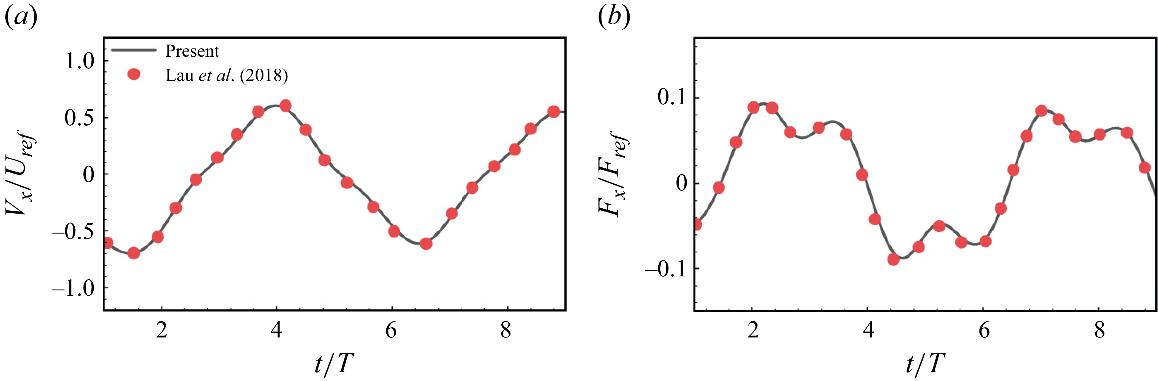
 (a)
 Vx
 (b)
 Fx
 Re=80
 I∗=0.1
 K=50
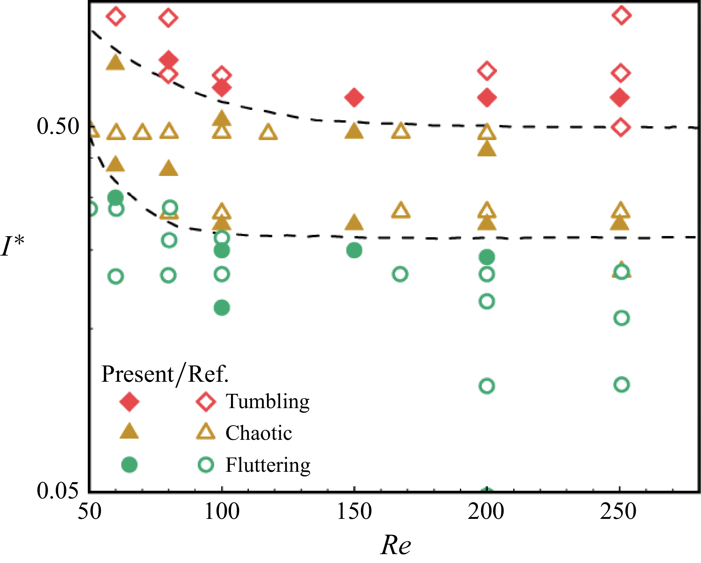
 (Re,I∗)
 K=0.05
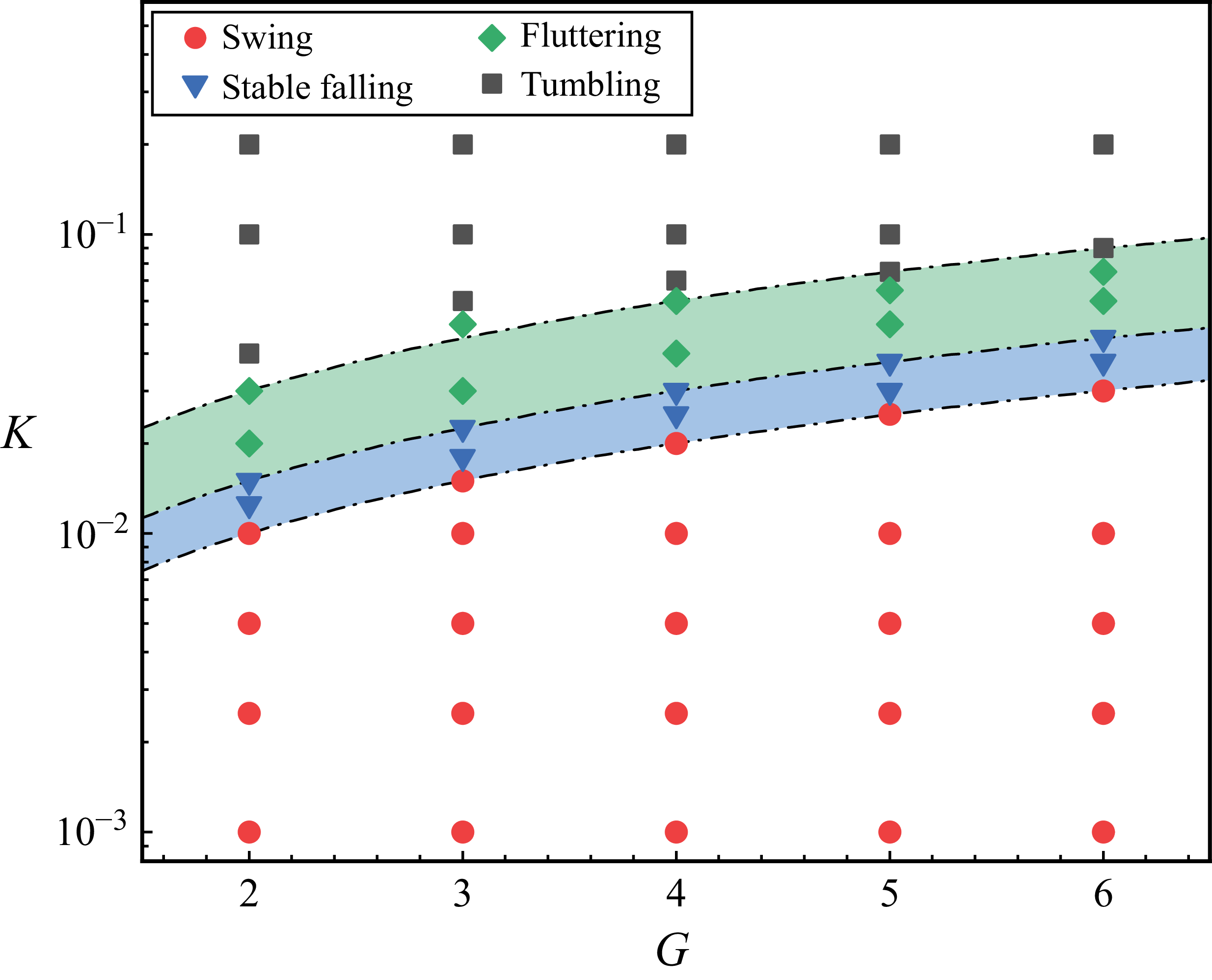
 (G,K)
 K/G

 i
 G=3,K=0.01
 ii
 G=2,K=0.015
 iii
 G=5,K=0.07
 iv
 G=5,K=0.09
 a
 p
 b
 c
 Tz
 d
 fn
 a
 d
 b
 c

 ωz
 a
 b
 c
 d

 (a)
 K
 (b)
 Vx
 Vy
 K
 G=2

 (a)
 f
 (b)
 Ic
 (c)
 Re
 (d)
 ReD
 K
 G
 fref=Uref/L

 Re
 G
 Kg

 (a)
 f∗
 (b)
 Ic
 (c)
 Re∗
 (d)
 ReD∗
 Kg
 G

 G=5
 Kg=0.014
 θ0
 a
 b
 τ

 θcr
 (a)
 K
 (b)
 Kg
 G

 G=4
 Kg=0.003
 (a)
 M=0.7
 (b)
 M=0.8
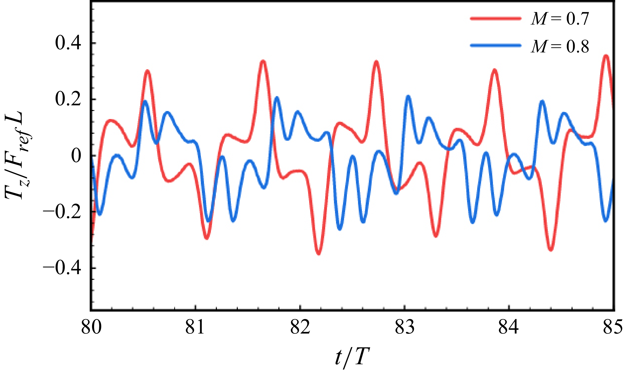
 Tz
 G=4
 Kg=0.003
 M=0.7
 M=0.8

 G,M,Kg
 Kg=0.002,0.003,0.004,0.005
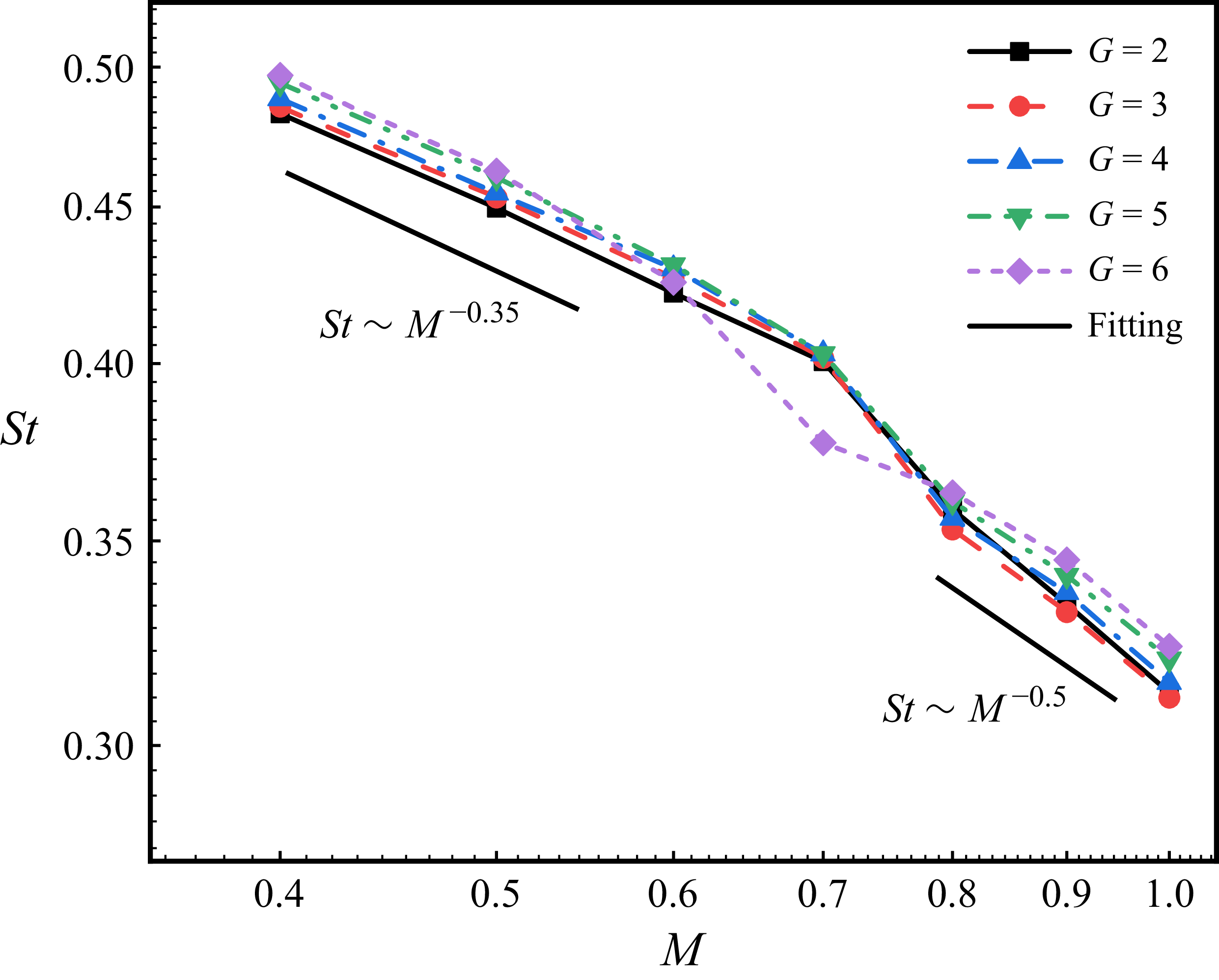
 St
 M
 G
 Kg=0.003
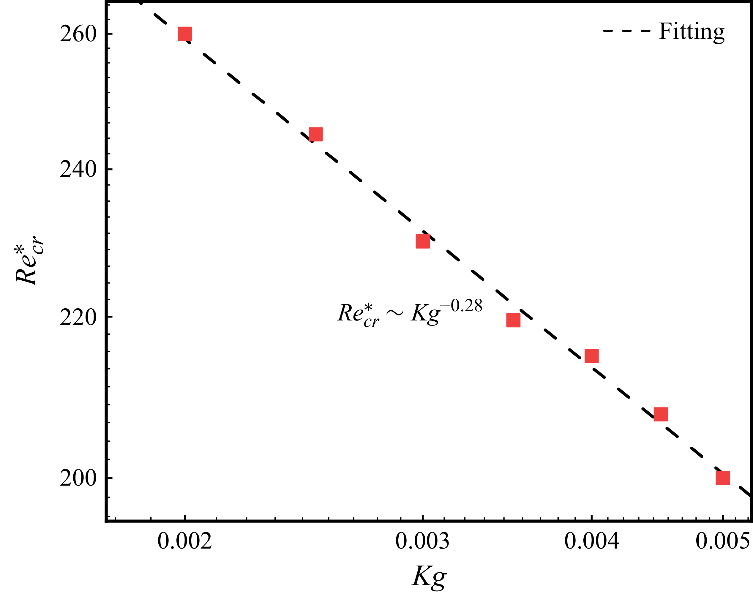
 Recr∗
 Kg

 i
 Ar=0.25,K=0.005
 ii
 Ar=0.25,K=0.03
 iii
 Ar=0.25,K=0.1
 iv
 Ar=1.0,K=1.0
 a
 b
 xz
 c
 yz
 G=4

 (G,K)
 a
 Ar=0.125
 b
 Ar=0.25
 c
 Ar=0.5
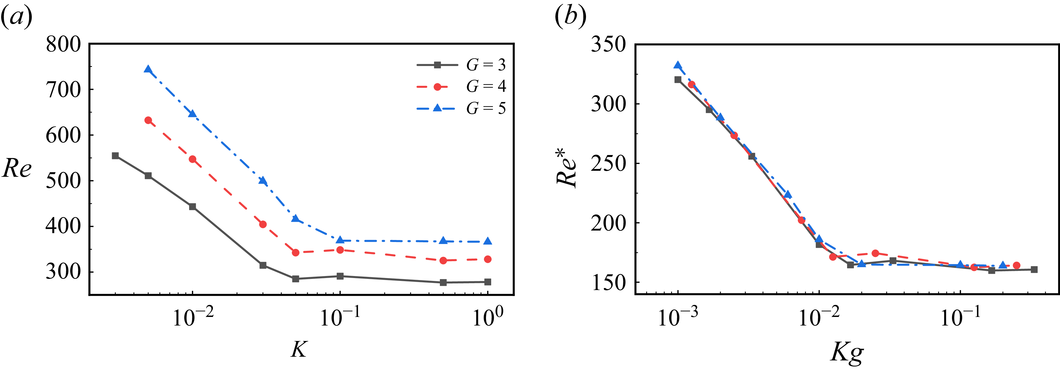
 Ar=0.25
 a
 Re
 K
 G
 b
 Re∗
 Kg

 G=4
 K=0.005
 a
 xz
 Ar=0.125
 Ar=0.25
 Ar=0.5
 b
 d
 b
 Ar=0.125
 c
 Ar=0.25
 d
 Ar=0.5

 Q=0.1
 (Q=(1/2)(‖Ω‖2−‖D‖2)
 Ω
 D
 z
 w
 a
 Ar=0.125
 b
 Ar=0.25
 c
 Ar=0.5

 Q=0.1
 z
 w
 a
 b
 M=0.5
 c
 d
 M=1.0
 G=4,Ar=0.5

 Ar=0.5
 K=0.03,G=4
 a
 b
 xz
 c
 xy

 Q=0.1
 z
 w
 Ar=0.125
 Ar=0.25
 Ar=0.5
 K=0.03,G=4

 G=4
 K=0.1
 a
 xz
 Ar=0.125
 Ar=0.25
 Ar=0.5
 b
 d
 p
 a
 b
 Ar=0.125
 c
 Ar=0.25
 d
 Ar=0.5

 Q=0.1
 z
 w
 Ar=0.125
 Ar=0.25
 Ar=0.5
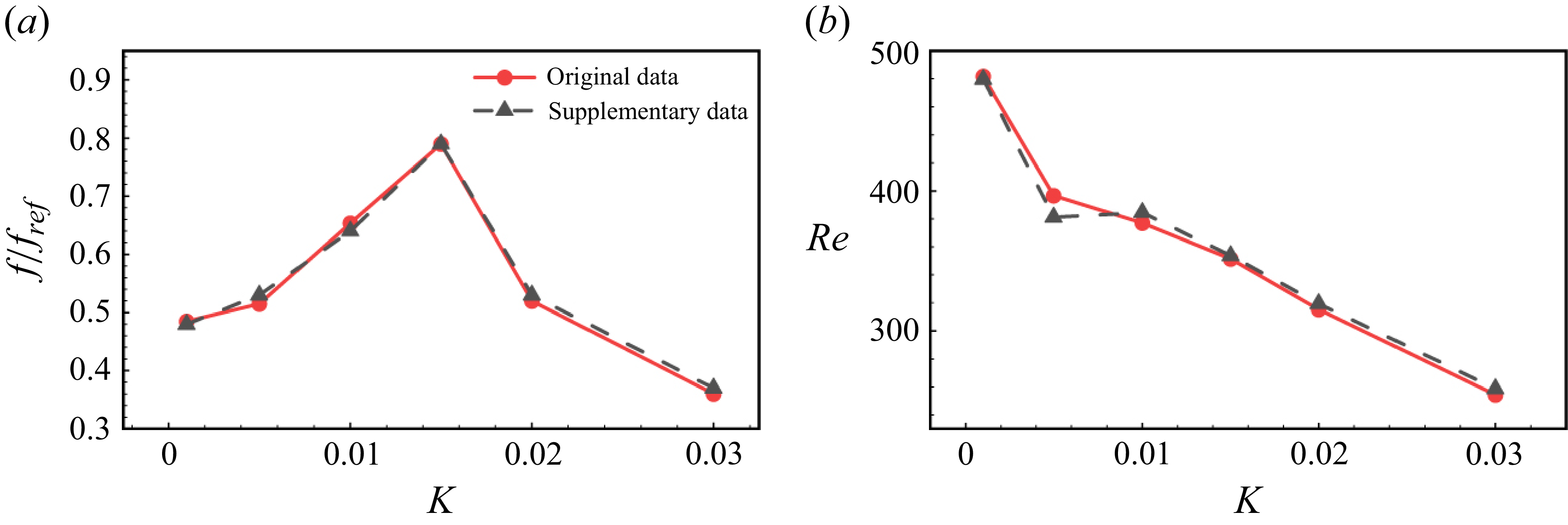
 G=3
 a
 f/fref
 b
 Re
 K
 10%


