1. Introduction

Energy-balance climate models (EBCMs) have been used widely in the past to study the sensitivity of the climate system. Reference BudykoBudyko (1969) and Reference SellersSellers (1969a) independently developed simple EBCMs with which the latitudinally varying response to some change in radiative forcing was evaluated. Since then, the treatment of the physical mechanisms in EBCMs has improved considerably (e.g. distinction between land, atmosphere and ocean and between snow, sea ice and land ice, and inclusion of seasonal cycle).

In recent years, it has been shown that with similar types of seasonal EBCMs, the present-day climate can be reproduced to a reasonably good approximation (e.g. Reference Peng, Chou and Arking.Peng and others, 1987; Reference HarveyHarvey, 1988b), which is a prerequisite for a correct simulation of climate sensitivity. Therefore, considerable effort is put into the simulation of present-day climate. Since the model is highly simplified compared to the actual climate system, discussions on detailed structures are not very meaningful. Therefore, we will limit ourselves to the large-scale features and compare these with observations.

Here, it will be demonstrated that the seasonal and latitudinal response introduced by the alberlo–temperature feed-back (α–T feed-back, hereafter) in this EBCM is qualitatively similar to that of GCMs (e.g. Reference Manabe. and Stouffer.Manabe and Stouffer, 1980). Three elements of the α–T feed-back will be distinguished: the dependence of sea-ice area, land snow area and snow/ice albedo on temperature. Only equilibrium results will be discussed in this paper.

2. Model Description

A zonally and vertically mean atmospheric layer is used, which is shown schematically in Figure 1. At the upper boundary, short-wave and long-wave radiative fluxes must balance while at the lower boundary the atmosphere exchanges radiative and turbulent energy with land and ocean. The processes in the atmosphere (i.e. radiation, horizontal heat transport and turbulent exchange of energy) are expressed in terms of surface air temperature (T _a). The zonal mean surface air temperature is governed by the following equation:

where r is the Earth’s radius, φ is latitude, D _a is the diffusion coefficient tor total atmospheric energy, H and L _E are the surface-air fluxes of sensible and latent heat, respectively, ΔL _a is the divergence of long-wave radiation, ΔS _a is the absorbed short-wave radiation, and C _p Δ_p/g is the thermal inertia of the atmosphere.

Fig. 1.

Schematic illustration of a Zonal band from the model, containing land, ocean, partial snow and sea-ice cover. S and L represent the short-wave and long-wave radiative fluxes, respectively. H and L_E are the vertical turbulent fluxes of sensible and latent heat at the surface, respectively. F_a and F₀ represent the total meridional heat fluxes in the atmosphere and ocean, respectively. F_z is the vertical heat flux between the upper ocean layer and the deep ocean

In a model with a vertically averaged atmosphere, only the radiative fluxes at the top of the atmosphere (TOA) and at the surface need to be evaluated. Therefore, the evaluation of the vertical radiation disitribution using sophisticated radiative transfer models is not necessary. A more convenient (and less time-consuming) method is to use a radiative transfer model to parameterize the TOA and surface fluxes in terms of all important variables. The solar radiative transfer through the atmosphere is determined mainly by the amount of water vapour and ozone, solar zenith angle, cloud amount, cloud optical thickness and surface albedo. Using the 24 band model of Reference Slingo. and Schrecker.Slingo and Schrecker (1982), the short-wave radiative fluxes are parameterized in terms of the quantities listed above. The long-wave fluxes are dependent on surface (air) temperature, water-vapour content, carbon-dioxide concentration, amount of ozone, cloud amount and cloud height. A broad-band emissivity radiative model is used to parameterize the long-wave fluxes in terms of the above-mentioned variables.

As in all EBCMs, the zonally averaged transport due to complicated, three-dimensional atmospheric motions is represented as a diffusive process in terms of the surface air temperature (first term on the righthand side of Equation (1)). According to Reference LorenzLorenz (1979) and Reference Stone and Miller.Stone and Miller (1980), the diffusive treatment of the meridional transport is applicable when one considers long-term averaged radiative forcing while using a seasonal model. The diffusion coefficient D _a represents the diffusion coefficient for the total atmospheric flux, which meridional distribution is taken from Reference HarveyHarvey (1988a).

With respect to zonal (land ocean) energy transport, the “infinite wind” mixing case is adopted here (Reference Peng, Chou and Arking.Peng and others, 1987). This means that one effective atmospheric layer Overlies the land as well as the ocean part of a latitude band.

The turbulent fluxes of sensible and latent heat between the surface and the atmosphere are evaluated according to standard aerodynamic bulk relationships.

The land fraction at a specific latitude is subdivided into three surface types: grass, forest and permanent land ice. This distinction is applied to account for the differences in albedo between the types and to incorporate the effect of masking albedo changes due to snowfall in snow-covered forests (Reference Ocrlemans. and van den Dool.Oerlemans and Van den Dool, 1978; Reference Robock.Robock, 1980). The coverage of these land surface types is fixed at its present-day distribution which means that the latitudinal shift of vegetation zones under varying climatic conditions is neglected. The fractional amount of snow present on land (a _s), equally distributed over the three surface types, is expressed as a function of the surface air temperature (Harvey, 1988a):

where T′_a = T _a + Γ_z is the surface air temperature corrected for the zonal mean surface elevation (z) with a global mean lapse rate Γ of −6.5 K km⁻¹. According to Reference Robock.Robock (1980), the snow/ice albedo is a function of surface temperature, cloudiness and zenith angle.

The zonal mean ocean circulation is schematically illustrated in Figure 2. The velocity field (u,w) is prescribed and kept fixed throughout the experiments. Upwelling takes place in the entire basin except for two areas at 50-70° S and 60-80° N where down-welling takes place; to complete the circulation, water flows poleward in the upper ocean layers and equatorward in the deep ocean. Thus, by transporting warm water poleward and cold water equatorward the thermohaline circulation effectively transports heat towards the poles. Further, a constant water depth of 4km is assumed. The temperature equation for the ocean reads (Reference Watts and Morantine.Watts and Morantine, 1990):

in which T _o is the ocean temperature, z is the vertical coordinate, f is the mean fractional basin width, u and w are the meridional and vertical velocity components, respectively, D _o (= 1.0 × 10¹¹ m² year⁻¹ in the Southern Hemisphere and 4.0 × 10¹¹ m² year⁻¹ in the Northern Hemisphere) and D _h (= 1.5 × 10¹⁰ m² year⁻¹) are horizontal diffusion coefficients, D _z (= 2.0 × 10³ m² year^−l) is the vertical diffusion coefficient, ΔL _o, ΔS _o, H _o and L _{E o} are the radiative and turbulent flux divergences in the upper ocean layer, and ρ _w, c _w and d _m the density, specific heat capacity and thickness, respectively, of the uppermost ocean layer. The first term on the righthand side of Equation (3) represents the poleward heat transport by gyres and eddies in the uppermost ocean layer. In the interior of the basin, horizontal heat transport is represented by the second term on the righthand side with diffusion coefficient D _h. The third term on the righthand side of Equation (3) represents all vertical mixing processes with diffusion coefficient D _z (assumed to be constant with depth and latitude). The last term on the righthand side of Equation (3) is the amount of radiative and turbulent energy received by the uppermost ocean layer. As standard case, a mean up-welling velocity w of 4 m year⁻¹ is assumed (Reference Hoffert, Callegari and Hsieh.Hoffert and others, 1980), which implies overturning rates of 17.2 and 20.2 Sv in the Northern (NH) and Southern Hemispheres (SH), respectively. However, the upwelling rate is assumed highest in the equatorial region and decreases linearly to zero at 50° S and 60° N (Fig. 2). Similarly, the down-welling velocities are assumed to increase linearly from zero to 70° S and 80° N, respectively. The meridional distribution of the horizontal velocity u then follows from the continuity equation

with the assumption of no advective heat fluxes through the lateral and vertical basin boundaries.

Fig. 2.

Schematic illustration of the zonal mean thermohaline circulation in the ocean. The arrows indicate the direction of the flow. S and L represent the short- and long-wave radiative fluxes, respectively. H and L_E represent the turbulent fluxes of sensible and latent heat between atmosphere and ocean.

Sea ice is incorporated in a purely thermodynamic way. Only areal sea-ice variations are considered since they are considered to be much more important than variation in thickness with respect to ihe surface energy budget. The momentum exchange of sea ice with atmosphere or ocean is neglected, which means that drifting of sea ice is not included. When the water temperature of the upper ocean layer (T _w) becomes smaller than the freezing temperature of water (T _f ≡ 271.22 K for a mean salinity of 35%), sea ice with a specified thickness (d _i = 2 m) starts to form. The fractional sea-ice cover (a _i) of a certain latitude band can be computed from conservation of energy

in which c _s is the latent heat of melting (= 3.35 × 10⁵ J kg⁻¹, ρ _i the density of ice (= 920 kg m⁻³, ρ _w the density of sea water (= 1000 kg m⁻³), c _w the specific heat capacity of sea water (= 3.9 × 10³J kg⁻¹ K⁻¹), and Δθ (= T _f–T _w) the undercooling temperature. Δθ can become positive after the “new” temperature is evaluated.

After applying Equation (5), the water and sea-ice temperature are set equal to T _f. If the fractional sea-ice amount becomes equal to 1.0 (i.e. the latitude band is entirely covered with sea ice), the sea-ice temperature (T _i) is allowed to decrease below T_f while the temperature of the underlying upper ocean layer remains equal to T _f. The sea-ice variations are due mainly to variations of the energy balance at the ocean surface. The energy supplied to the uppermost ocean layer covered by sea ice through advection and diffusion in the ocean is implicitly equal to the energy flux through the base of the sea-ice layer and is therefore used to warm/cool the sea ice. Obviously, the melting process is rather similar to the freezing process described above.

The albedo of sea ice is taken similar to that of land ice with respect to its dependence on snow cover, zenith angle, surface temperature and cloudiness. The amount of snow covering the sea ice is governed by Equation (3) using sea-ice temperatures.

In the meridional direction, a 5° grid distance is used in the ocean and atmosphere. The ocean is subdivided into six vertical layers with increasing layer thickness towards the bottom (100, 317, 544, 776, 1012 and 1251 m). The meridional distribution of cloud amount is prescribed according to observations, while the globally Uniform cloud optical depth is used to tune the model to its present-day state.

3. Simulation of Present-Day Climate

The characteristics of the differences between simulated and observed current-climate state will be discussed. The meridional distribution of the annual, zonal mean surface air temperature and its seasonal range are shown in Figure 3. The overall agreement seems to be good, although the model somewhat underestimates the surface air temperatures in the region 10-45° N (the maximum difference is about 4° C). Temperatures over the Antarctic continent are significantly lower than over the North Polar basin (even when corrected to sea-level temperatures), as correctly simulated by the model. Due to the large land masses in the NH, the amplitude of the seasonal cycle of air temperature is largest there. The poleward enhancement of the seasonal temperature range, due to the poleward increase in seasonal amplitude of incident solar radiation, seems to be captured by the model, although the small-scale structures are not, possibly due to the use of “infinite-wind” zonal atmospheric heat transport.

Fig. 3.

Zonal and annual mean surface air temperature and its seasonal range (solid line). Dots are observations given by Reference Wanen and Schneider.Warren and Schneider (1979).

The model successfully reproduces the seasonally varying snow cover on land. On the other hand, some problems exist with respect to the seasonal behaviour of sea-ice amount: in the NH, the seasonal range is overestimated while in the SH it is underestimated. The phase of the annual cycle seems to be simulated correctly, with extremes in sea-ice cover in February-March and August-September. The simulation of the latitudinal distribution of annual mean surface albedo seems fairly good as compared with values from Reference Robock.Robock (1980), with maximum discrepancies of about 0.03. Global mean values of the radiation budget are shown in Table 1 together with estimates from Reference SellersSellers (1969b), The largest discrepancies seem to occur in the long-wave region. However, differences between the model and observations are relatively small and of the order of the accuracy of the observations.

Table 1.

Observed (Sellers, 1969b) and model-generated mean annual, globally averaged radiative terms (W m⁻²)

Concerning the transport in the atmosphere, the model seems to be able to reproduce the main features, as indicated in Figure 4: maximum values of about 3 × 10¹⁵ W at 45° in both hemispheres. Obviously, these characteristics are imposed mainly by the choice of transport formulation and by the meridional distribution of the atmospheric diffusion coefficient (D _a). According to the (widely varying) observations, the maximum oceanic transport takes place at lower latitudes. This aspect is reproduced by the model due to the contribution of the meridional overturning (transport hereby is proportional to the meridional mass flux and temperature difference between top and bottom model ocean layer). Therefore, the inclusion of an overturning mechanism, simple as it may be, improves the meridional distribution of ocean heat transport compared to models which only take diffusive ocean transport into account. The eddy/gyre transport contributes little to the total oceanic transport, especially in the SH. This causes the total oceanic heat flux to be largest in the NH. However, the total ocean heat transport is still only hall of the atmospheric transport.

Fig. 4.

Annual and zonal mean meridional energy transport in atmosphere and ocean. Minimum and maximum estimates of total ocean transport are from Reference Hsuing.Hsuing (1985) and Reference Carissimo, Oort and Vonder Haar.Carissimo and others (1985), respectively. In the lower panel, estimates of atmospheric transport are taken from Carissimo and others (black squares) and Reference Oort and Vonder Haar.Oort and Vonder Haar (1976) (white squares)

4. The Albedo-Temperature Feed-Back

In order to quantify the contribution of each element of the α–T feed-back mechanism to the actual response, three separate effects are considered: (1) the dependence of sea-ice cover on temperature (referred to as sea-ice area feed-back, hereafter), (2) the dependence of snow cover on temperature (snow area feed-back), and (3) the dependence of snow/ice albedo on temperature (snow-albedo feed-back). Four additional model versions have been constructed in which the element considered is fixed at its latitudinally and seasonally varying present-day distribution. The five models considered are:

• A₁ Full α–T feed-back

• A₂ Sea-ice area fixed

• A₃ Land snow area fixed

• A₄ Snow/ice albedo fixed

• A₅ No α–T feed-back (i.e. A₂ + A₃ + A₄).

A uniform decrease of 2% in solar insolation at TOA is applied. The latitudinal and seasonal distribution of change in surface air temperature for the five models is presented in Figure 5. The annual mean response for the various models is shown in Figure 6a. Obviously, the strong seasonal cycle in the response of model A₁ in the polar regions is due entirely to variations in sea ice, since the response of model A₂. shows no seasonal behaviour. All models including sea-ice variations (A₁, A₃ and A₄) have this typical seasonal “sea-ice-induced” response, which can be characterized by a large seasonal variation in the response in surface air temperature of the polar regions. It is caused by enhanced heating of the ocean in summer as a result of reduced sea ice. The additional heat is released to the overlying atmosphere in winter, also due to reduced sea-ice cover (Reference Manabe. and Stouffer.Manabe and Stouffer, 1980; Reference HarveyHarvey, 1988b). If the sea-ice area is fixed (model A₂), the polar amplification of sensitivity is virtually absent, similar to the response in the absence of the α – T feedback (model A₅).

Fig. 5.

Latitudinal and seasonal distribution of atmospheric temperature change resulting from a 2% decrease in solar constant for models A₁ – A₅. Light-grey and dark-grey areas represent temperature changes of less than 2° C and more than 4° C, respectively

Fig. 6.

Meridional distribution of the change in zonal and annual mean (a) surface air temperature and (b) net solar radiation at TOA, resulting from a 2% decrease in solar constant for models A₁ – A₅. Also shown in (b) as “initial forcing” is the decrease in the TOA solar radiation just after the solar constant is reduced by 2% and without any climate feed-backs

With sea ice fixed there is a slight increase in temperature change which peaks in the mid-latitudes between 30° and 60° N (Fig. 6a). At these latitudes, where spring and autumn snow cover is still significant, net change in TOA solar radiation is largest, as can be inferred from Figure 6b. In the SH, changes in solar radiation and temperature due to variations in snow cover are virtually absent since land snow cover outside the Antarctic continent does not exist in the present-day climate. The low sensitivity in the NH is due to the fact that, in the present-day state, snow Cover is small in summer when changes in incident solar radiation are largest. As a result, the snow area feed-back is relatively weak compared to the sea-ice area feed-back. Although sensitivity induced by the snow area feed-back alone is small, it effectively enhances the sensitivity due to sea-ice area feedback in the NH, as can be inferred from Figures 5 and 6 when the results of A₁ and A₃ are compared.

Unexpectedly, the omission of the dependence of the snow/ice temperature on albedo (model A₄) enhances the sensitivity in the NH, in contrast to the response in the SH. Presumably, this is due to a sea-ice-induced shift in seasonal cycle of the surface temperature. However, since this is only a minor effect it will not be extensively discussed here.

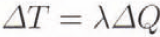
In order to quantify the magnitude of these feed-back mechanisms, a linear feed-back analysis is adopted here. Generally, the change in global mean surface air-temperature (ΔT) resulting from an initial change in TOA radiative forcing (ΔQ) can be written as:

where λ is referred to as the sensitivity parameter. In the absence of internal feed-backs, the sensitivity parameter (λ₀) can be estimated from the derivative of the spectrally integrated Planck function at the effective radiation temperature (T _ep):

which, for present-day value of L (Table 1) gives λ₀ = 0.266 (W m⁻² K⁻¹)⁻¹. With the inclusion of feed-back mechanisms, Equation (6) can be expressed as:

where subscript i denotes feed-back mechanism i. It is generally assumed that the contributions to λ⁻¹ from the individual feed-back mechanisms combine linearly for small ΔQ. Furthermore, it is assumed that the λ_i ⁻¹ are independent of whatever other feed-back mechanism is present. Note, however, that the temperature response does depend on the presence of feed-back mechanisms, which implies that these can amplify each other with respect to the temperature response, as can be inferred from Equation (8). The values λ_i ⁻¹ for each feed-back i can be easily evaluated from the difference of the total λ with and without feed-back i operating. Thus, the λ_i ⁻¹ for each element of the α – T feed-back can be obtained from the global mean temperature response of models A₁ – A₅. The resulting values of λ_i ⁻¹ for a 2% decrease in solar constant (S _o) are shown in Table 2. Note that λ_i ⁻¹ is negative for a positive feed-back.

Table 2.

Global mean values of the inverse sensitivity parameter associated with individual feed-back processes for a 2% decrease in solar constant

The combined water-vapour – temperature feed-back for short-wave and long-wave radiation is larger than the total α – T feed-back, which amounts to λ _{α – T} ⁻¹ = −0.77 W m⁻² K⁻¹. It must be noted, however, that the sensitivity due to the water-vapour – temperature feed-back (λ_H2O ⁻¹) could not be evaluated independently. It was estimated as being the difference between the value of λ produced by the “no α – T feed-back model” (model A₅) and λ ₀. Reference CessCess (1989) estimates λ_H2O ⁻¹ = −1.2 W m⁻² K⁻¹ which agrees reasonably well with the value linmd here.

As discussed above, global sensitivity due to sea-ice area feed-back is much larger than that due to snow area feed-back, whereas the snow/ice albedo feed-back is relatively weak. These results compare reasonably well with the values presented by Reference Robock.Robock (1983). Using a seasonal EBCM he obtained for the snow area, sea-ice area and snow/ice albedo values of λ_i ⁻¹ of −0.07, −0.45 and −0.13 W m⁻² K^−l, respectively. Harvey (1988b) confirms our conclusion that the snow/ice albedo feedback has very little effect on global sensitivity. Reference CessCess and others (1991) compare snow area feed-back in 17 GCMs by perturbing the sea surface temperature for a perpetual April simulation. Without cloud feed-backs, the model-mean clear-sky inverse sensitivity parameter is about −0.37 W m⁻² K⁻¹ with the extremes being −0.03 and −0.90 W m⁻² K⁻¹.

Table 3 shows the inverse sensitivity parameter λ_{α – T} ⁻¹ for the total α – T feed-back as determined in various modelling studies. Our model agrees roughly with three of the referred models. The two other models predict an α – T feed-back approximately only half as strong as in the other four models. This fact illustrates the need for more studies on the α – T feed-back. However, it may be safe to state that the total α – T feed-back is significantly weaker than the total water-vapour – temperature feed-back with respect to the global mean response for the present-day climate.

Table 3.

The inverse sensitivity parameter for the total α-–T feedback λ_α–T ⁻¹ (W m⁻² K⁻¹) as determined in various models for forcings of 2 × CO₂ or S₀ ± 1-2%. Adopted from Harvey (1988b)

For larger excursions off the current climate, the total global sensitivity shows a marked asymmetry, as shown in Figure 7. This is due mainly to a stronger α – T feed-back in colder climates, which is the main cause for λ to increase as S ₀ decreases. In colder climates, high reflective areas extend into regions with high insolation, which dramatically increases the change in TOA radiation balance resulting from a change in surface albedo. Therefore, the sensitivity of the model climate depends strongly on the state itself, which emphasises the importance of accurately simulating the present-day climate in studies concerning climate sensitivity.

Fig. 7.

Values of a sensitivity parameter λ for a wide range of changes in solar constant

5. Conclusions

In this paper, the albedo – temperature (α – T) feed-back is analyzed with a coupled EBCM ocean advection diffusion model. In particular, its impact on the latitudinally and seasonally varying and global mean temperature response is discussed. The α – T feed-back is subdivided into three components, which are all dependent on temperature: (1) sea-ice area, (2) land snow-cover area, and (3) snow/ice albedo. The enhancement of the global sensitivity caused by the n α – T feed-back is due mainly to sea-ice area, feed-back. The snow area feed-back appears to be only half as strong as the sea-ice area feed-back while the snow/ice albedo feed-back is very small. Although the α – T feed-back introduces enhanced sensitivity of the polar regions, it is weaker than the water-vapour – temperature feed-back with respect to the global mean response. Comparison with other (types of) models shows that the global mean sensitivity produced by the α – T feed-back is probably well reproduced in the present model, although its interaction with other feedbacks not included in this model (e.g. cloud feed-backs may significantly change these results.