INTRODUCTION
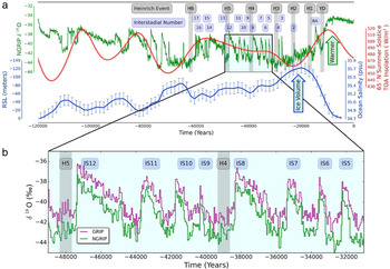
During the most recent glaciation-deglaciation cycle of the Late Quaternary ice age, repeated partial deglaciations of the continental ice sheets that were then adjacent to the North Atlantic Ocean episodically disgorged “armadas” of icebergs that, upon melting, deposited layers of ice-rafted debris (IRD) onto the ocean floor. These sediment layers, first identified by Hartmut Heinrich (Heinrich, Reference Heinrich1988), provided the initial evidence for the existence of what came to be called “Heinrich events” (H or HE). These events are labeled H1, H2, etc. with H1 being the most recent, in the oxygen isotopic variability measured in Summit Greenland ice cores shown in Figure 1 on the time scale inferred from the North Greenland Ice Core Project (NGRIP) ice core using various methods (Andersen et al., Reference Andersen, Azuma, Barnola, Bigler, Biscaye, Caillon and Chappellaz2004). The oscillations of ice core oxygen isotopic variability labeled IS1, IS2, etc. are interstadials that have come to be called Dansgaard-Oeschger (D-O) oscillations. These D-O oscillations follow H-events, which strongly suggests that the H-events are the cause of these oscillations. The opposite notion—that D-O oscillations might, in fact, be the cause of H-events—was also entertained in the early literature, but these D-O cycles have been recently established as being caused by H-events, (Peltier and Vettoretti, Reference Peltier and Vettoretti2014; Peltier et al., Reference Peltier, Ma and Chandan2020), thereby demonstrating the primacy of the H-event mechanism.
(color online) The relationship between relative sea level and the oxygen isotopic anomaly δ 18O is shown from Marine Oxygen Isotope (MIS) stage 5 to the present day. Note that the modelled sea level data have been inverted to make the relationship between ice volume and ocean salinity more easily observed. The relative sea level and salinity are calculated based on benthic foraminifera isotopic records (Waelbroeck et al., Reference Waelbroeck, Labeyrie, Michel, Duplessy, McManus, Lambeck, Balbon and Labracherie2002). The deep ocean salinity is known to be higher under glacial conditions (Boyle and Keigwin, Reference Boyle and Keigwin1987; Adkins and Schrag, Reference Adkins and Schrag2001; Adkins et al., Reference Adkins, McIntyre and Schrag2002), and this is reflected in the figure. Figure adapted from Peltier and Vettoretti (Reference Peltier and Vettoretti2014). GRIP: Greenland Ice Core Project; NGRIP: North Greenland Ice Core Project; TOA: Top of atmosphere.

Much effort has been invested in attempts to understand the dynamical mechanism underlying the occurrence of the H-process. Two aspects of the observations have received the most intense focus in the search for understanding: event duration and the pseudo-periodicity of their occurrence on a time scale of approximately 7000 years (e.g., MacAyeal, Reference MacAyeal1993; Bond and Lotti, Reference Bond and Lotti1995; Rohling et al., Reference Rohling, Marsh, Wells, Siddall and Edwards2004). As yet, no proposed explanation has proven to be entirely satisfactory. Insofar as the geographical region of partial ice sheet instability is concerned, the Hudson Strait has long been hypothesized to be the primary source of the icebergs that were responsible for the transport of the IRD that define individual H-events (e.g., Dowdeswell et al., Reference Dowdeswell, Maslin, Andrews and McCave1995). This hypothesis has been strengthened via provenance analyses of the IRD within the Heinrich layers, which determined that the lithic fragments involved were sourced from both the Churchill and Superior geological provinces that exist, respectively, on the northern and southern flanks of the Hudson Strait (Bond et al., Reference Bond, Heinrich, Broecker, Labeyrie, McManus, Andrews and Huon1992; Gwiazda et al., Reference Gwiazda, Hemming, Broecker, Onsttot and Mueller1996b). However, these same provenance analyses determined that not all H-events produced the same signature in the deep-sea sedimentary cores that contained their stratigraphic expression. Notably, H3 and H6 appear to differ markedly from the others. In what follows, we will refer to H-events 1, 2, 4, and 5 as “Laurentide Heinrich Events” (LHEs) and H-events 3 and 6 as “anomalous HEs.” Note that in much of the cited literature, the Younger-Dryas (YD) is erroneously referred to as H0, but this event has no expression in a layer of IRD within the sedimentary cores raised from the so-called Ruddiman Belt of the North Atlantic Ocean (Ruddiman and McIntyre, Reference Ruddiman and McIntyre1981; Andrews et al., Reference Andrews, Jennings, Kerwin, Kirby, Manley, Miller, Bond and MacLean1995; Rashid et al., Reference Rashid, Piper and Flower2011). This early misconception was resolved when the YD was determined to have been predominantly caused by a release of meltwater into the Arctic Ocean through the McKenzie River outlet beginning at approximately 12,800 years ago (Tarasov and Peltier, Reference Tarasov and Peltier2005; Peltier et al., Reference Peltier, Vettoretti and Stastna2006; Murton et al., Reference Murton, Bateman, Dallimore, Teller and Yang2010; Keigwin et al., Reference Keigwin, Klotsko, Zhao, Reilly, Giosan and Driscoll2018) from proglacial lakes that existed on the southern and western edges of the Laurentide Ice Sheet during its deglaciation. These analyses corrected the original argument by Broecker et al. (Reference Broecker, Kennett, Flower, Teller, Trumbore, Bonani and Wolfli1989) that the freshwater outflow that triggered the YD had entered the Atlantic through the St. Lawrence River outlet. An additional H-event, referred to as H5a, occurring between H6 and H5 has also been suggested (Rashid et al., Reference Rashid, Hesse and Piper2003b; Stoner et al., Reference Stoner, Channell and Hillaire-Marcel1998). If such an event did in fact occur, H-events would have occurred very approximately every 7000 years since H6. This estimate of recurrence time is clearly very approximate.
In the ocean floor sedimentary record, the characteristic signature of all HEs is an increase in the relative concentration of IRD to other materials in the sediment column. This is associated with two characteristics of the H-signal: an increase in the absolute amount of IRD present in the sediment and a decrease in foraminiferal abundance. In the case of LHEs, both of these characteristics appear to occur simultaneously. In the case of anomalous HEs, however, a foraminiferal depletion is observed, but no significant increase in the absolute amount of IRD is observed. Furthermore, the detrital carbonate present in H3 is at a lower concentration than in other HE layers. Furthermore, Sr and Nd isotopic analyses of the bulk silicate fraction found in H3 indicate a different origin, and the K/Ar ages of the fine fraction associated with H3 taken from cores raised in the eastern North Atlantic are similar to the background glacial sediment; in contrast, the dates for the fine fraction associated with other H-events differs substantially from the background. These differences, further described by Gwiazda et al. (Reference Gwiazda, Hemming and Broecker1996a), indicate that the source of iceberg flux responsible for anomalous HEs might differ from that responsible for LHEs.
It is important to note that there has been a longstanding debate in the literature as to whether the source of icebergs for anomalous HEs was exclusively eastern Atlantic, or if the Hudson Strait ice stream also or even solely contributed. Rashid et al. (Reference Rashid, Hesse and Piper2003a) suggest that the Hudson Strait is the source of the iceberg flux responsible for H3, but Hemming (Reference Hemming2004) argues that if the Hudson Strait did contribute, it was not the dominant source. More recently, Andrews and Voelker (Reference Andrews and Voelker2018) suggested that all HEs are primarily sourced from the Hudson Strait, though the degree to which other ice streams might have also contributed has not been satisfactorily addressed in the literature. Specifically, the Fennoscandian ice sheet (Álvarez-Solas et al., Reference Álvarez-Solas, Montoya, Ritz, Ramstein, Charbit, Dumas, Nisanciogl, Dokken and Ganopolski2011) and the British Isles ice sheet (Scourse et al., Reference Scourse, Hall, McCave, Young and Sugdon2000) have been suggested as possibly having been involved in H-events, though the nature of this involvement and temporal relationship to the instability in the Hudson Strait has not been satisfactorily determined.
The principal reason for confusion about the source of anomalous HEs is the lack of a strong signal in the Labrador Sea sedimentary record that can be temporally correlated with H3. Nevertheless, the possibility that there were at least two different sources for the required flux of icebergs poses a problem for general theories of HEs. Either there are two unrelated processes, both of which happen to produce iceberg flux in the North Atlantic, or a single mechanism must exist by which different ice streams or ice sheets are rendered unstable while still producing a pseudo-periodicity of 7000 years. It is important to note that the theory of the H-process advanced by Velay-Vitow et al. (Reference Velay-Vitow, Peltier and Stuhne2020) also includes an interpretation of this very approximate 7000-year time scale through its reliance on the glacial isostatic adjustment of the ice streambed in response to the instability associated with a Heinrich event. This rebound process enables the bed slope to recover, which allows the ice stream to reform even in the presence of a high-amplitude tide at the outlet of Hudson Strait. Nevertheless, there is some indication that the European ice sheets may have contributed to iceberg flux during HEs; this relates to the existence of the so-called “precursor” events that produce signatures in the sedimentary record prior to only H1 and H2 (Grousset et al., Reference Grousset, Cortijo, Huon, Hervé, Richter, Burdloff, Duprat and Weber2001). Between these precursor events to LHEs and anomalous HEs, the European ice sheets are potentially involved in a majority of HEs.
Following the work by Velay-Vitow et al. (Reference Velay-Vitow, Peltier and Stuhne2020), we investigate the possibility that all HEs are tidally triggered and thereafter are continuously forced by the same mechanism. This assumption does not rule out the possibility that some other cause, or combination of causes, may have played a role in the onset of H-events, but a single mechanism would appear to be more likely given the repeated nature and quasi-regularity of H-events. In the case of H3 specifically and anomalous HEs in general, we consider the possibility that an ice stream in the eastern sector of the North Atlantic was rendered unstable and injected a flux of icebergs into the Atlantic Ocean. The melting of these icebergs would then result in sediment deposition over the Ruddiman belt. There exists the possibility that a marine-terminating ice stream in the western sector of the North Atlantic, for example those that existed in Cumberland Sound or Frobisher Bay (Margold et al., Reference Margold, Stokes and Clark2015), may have contributed. There also exists the possibility that an ice stream that drained the Greenland Ice Sheet or Iceland ice sheet could have contributed. Detailed investigation of these possibilities is beyond the scope of this study, which was intended to explore only eastern-sector North Atlantic contributions. Western sector possibilities will be examined in future work concerning possible contributions to H-events from additional sources. The possibility also exists that an ice stream grounded on the Greenland-Iceland-Faroe ridge may have contributed, but we are limited in this study to ice streams whose existence is supported by the ICE7G NA (VM7) model of ice-loading history, which is not especially well constrained in that area. These possibilities are beyond the scope of this study and are intended to be examined in future work.
In this study, we examine three eastern-sector locations: a plausible Barents Sea ice stream, the Norwegian ice stream, and the Irish Sea ice stream. We determine that for each of the cases examined, deglaciation via the same mechanism as that proposed for H1 is unlikely, and furthermore, that the effect of the modeled deglaciation on the western North Atlantic M2 tidal resonance is negligible in all three cases. The most likely location for a tidally triggered marine ice sheet instability associated with anomalous H-events is the Hudson Strait. Of the eastern-sector North Atlantic candidates, the Irish Sea ice stream remains worthy of some consideration.
METHODOLOGY
The technical details of the global ocean model herein employed in the investigation of the viability of the tidally forced ice stream instability mechanism for H-events are discussed in this section. This is the same model as used by Velay-Vitow et al. (Reference Velay-Vitow, Peltier and Stuhne2020) to establish the role that the oceanic tides may have played in triggering and thereafter continuously forcing H1; this model is briefly revisited in this Methods section. A full discussion of the model and the aquaplanet benchmarks used to test it can be found in Salehipour et al. (Reference Salehipour, Stuhne and Peltier2013), where it was also shown to correctly reproduce the amplitude and phase of the primary tidal constituents of the modern ocean as determined by the Topex/Poseidon altimetric observations. We also discuss the discontinuous Galerkin (DG) model, as well as the modeling choices made concerning H3. We do not model H6 separately, as both the sedimentological and ice thickness data are of significantly higher quality in the case of H3. Beyond this, the dominant factors that control the amplitude of the M2 tidal constituent in the North Atlantic are the positions of the continents, the margins of grounded ice sheets, and the regional sea level, none of which are assumed in the ICE-7G NA (VM7) reconstruction to have changed in a significant way between H3 and H6. We have also limited our analysis to the M2 tidal constituent, as it is an order of magnitude larger than any other tidal constituent and has been shown to be the tidal constituent most affected by the deglaciation of the Hudson Strait ice stream (Velay-Vitow et al., Reference Velay-Vitow, Peltier and Stuhne2020). While constructive interference between the M2 tide and other tidal constituents would create a condition of increased tidal range, for this to be meaningful the M2 tidal constituent itself would need to increase dramatically in the area adjacent to one of the proposed ice streams, as is observed in the Hudson Strait.
The discontinuous Galerkin model of shallow water tides
The DG model of shallow water tides was first described by Salehipour et al. (Reference Salehipour, Stuhne and Peltier2013) where it was benchmarked against the aquaplanet test cases 2 and 5 described by Williamson et al. (Reference Williamson, Drake, Hack, Jakob and Swarztrauber1992) for shallow water models as well as via the simulation of the evolution of a baratropically unstable jet due to perturbation of an initially stable zonal flow, as was originally proposed as an additional shallow water theory benchmark by Galewsky et al. (Reference Galewsky, Scott and Polvani2004). The DG model has also been validated against the TOPEX/Poseidon data for the M2 and K1 tidal constituents under modern conditions, and the results for the M2 and K1 tidal constituents at last glacial maximum (LGM) have been presented by Griffiths and Peltier (Reference Griffiths and Peltier2008, Reference Griffiths and Peltier2009). The methodology, briefly summarized, involves using the 2D spherical shallow-water tidal equations (Egbert et al., Reference Egbert, Ray and Bills2004) in their flux form as:

Here Q represents all conserved quantities, F = [Fx, Fy, Fz] is the flux term, S is the source term, and Q = [φ φ u]T,

and

Here φ = gh(x, t) is the geopotential height, ρ is the density, g is the gravitational acceleration, φu is the depth-averaged horizontal transport, u = (u, v, w)T is the velocity vector, ê g is a unit vector pointing normal to the surface of the sphere, f is the Coriolis parameter, φeq is the equilibrium tidal variation induced by astronomical bodies, φsal is the influence on the tide due to gravitational self-attraction and loading, and φs is the equilibrium geopotential height. The fluid depth, h(x, t), can be expressed as the sum of the depth measured from the undisturbed ocean surface to the sea floor hs(x, t) and free-surface elevation ζ(x, t). As the velocity vector is expressed in Cartesian coordinates, it must be explicitly constrained to the sphere using the same method based on the use of projection matrices as was employed by Williamson et al. (Reference Williamson, Drake, Hack, Jakob and Swarztrauber1992). DIT and DBL are the dissipation due to internal tides and the ocean floor boundary layer, respectively.
The form of the tidal variation due to the gravitational attraction of distinct astronomical bodies, the influence on the tide due to self-attraction and loading (Accad and Pekeris, Reference Accad and Pekeris1978), as well as boundary layer (Taylor, Reference Taylor1919) and internal tidal dissipation (Griffiths and Grimshaw, Reference Griffiths and Grimshaw2007) used in this investigation are identical to those used by Velay-Vitow et al. (Reference Velay-Vitow, Peltier and Stuhne2020) following the work by Salehipour et al. (Reference Salehipour, Stuhne and Peltier2013). They are given respectively by:


and

Here θ and λ are latitude and longitude, A is the equilibrium amplitude, ω is the tidal frequency, and κ is the appropriate surface load Love number (Farrell, Reference Farrell1972). These values can be found in table 1 of Arbic et al. (Reference Arbic, Garner, Hallberg and Simmons2004). Finally, N̄̄2 is the vertically averaged buoyancy frequency of the ocean. For the purposes of this analysis, the longitude- and latitude- dependent vertical average of the buoyancy frequency of the oceans is assumed to be identical to that for LGM obtained on the basis of a coupled climate model simulation of glacial conditions (Vettoretti and Peltier, Reference Vettoretti and Peltier2013). Though the question of deep stratification has not been completely resolved in the literature, the DG model employed is only very weakly dependent on the buoyancy frequency. As such, the exact choice of how to represent these frequencies does not affect our results.
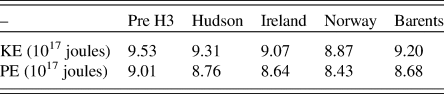
Kinetic and potential energies of the M2 tidal constituent prior to and after Heinrich event 3 (H3).

Review of Velay-Vitow et al. (Reference Velay-Vitow, Peltier and Stuhne2020)
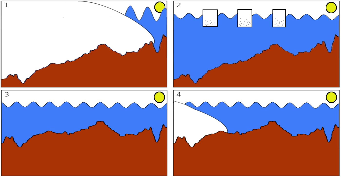
Velay-Vitow et al. (Reference Velay-Vitow, Peltier and Stuhne2020) advance a model of tidally triggered marine ice stream instability as a possible explanation for H-events. In this model, the strait is initially assumed to be filled with an ice stream that is responsible for draining a significant region of the eastern Laurentide Ice Sheet. Additionally, the M2 tidal constituent is in a strongly enhanced state of resonance in the North Atlantic. Constructive interference of the M2 and S2 tidal constituents (the spring-neap cycle) is suggested to be responsible for triggering an ice stream instability in the Hudson Strait, which proceeds rapidly inland until it is arrested at Southampton Island. The underlying crust, depressed under the weight of the ice stream, must be of sufficiently steep retrograde slope for this instability to propagate (Schoof, Reference Schoof2012). With the weight of the ice removed, the floor of Hudson Strait and the surrounding region begins to rebound under the action of the isostatic adjustment process (e.g., Peltier et al., Reference Peltier, Argus and Drummond2015, for recent review) until such a time as the slope is sufficiently reduced to allow a re-advance of the Hudson Strait ice stream to occur. This ice stream, no longer prone to tidal destabilization, remains in place and continues to thicken until the weight of the reestablished ice stream is able to depress the Earth's crust sufficiently to render the ice stream susceptible to a further deglaciation event. It is in this fashion that the authors imagine the approximately 7000-year pseudo-periodicity of H-events to be achieved. This process is illustrated by the cartoon in Figure 2. The proposed model is suggested to be an example of Self Organized Criticality (SOC), a phenomenon in which non-linear systems may be characterized by the existence of a point of instability in the space of its parameters, a point which is also an “attractor” of its dynamics. That is to say, non-linear systems are continuously drawn toward a state in which they experience a rapid change in behavior.
(color online) In panel one, the strait is shown prior to a Heinrich event; the underlying crust slopes up to the Atlantic, and the strait is filled with grounded ice. The North Atlantic resonance is strong, and the amplitude of the tides is large. In panel two, a Heinrich event has occurred, and icebergs laden with ice-rafted debris are released into the Atlantic Ocean. As the ocean is no longer in a state of maximum tidal resonance, the amplitude of the tides is decreased. Panel three shows the crust rebounding as it is no longer depressed under the weight of the ice. In panel four, the ice begins to reform as the slope of the underlying crust is no longer sufficiently steep to prevent ice stream readvance. Note that the floating ice stream that could potentially exist at the margin of the ice stream is not shown. Figure and caption adapted from Velay-Vitow et al. (Reference Velay-Vitow, Peltier and Stuhne2020).

This concept was introduced into the physics literature by Bak and Tang (Reference Bak and Tang1989) who discussed it in terms of a “sand pile” analogy. In this thought experiment sand grains are continuously dropped onto a horizontal surface. Eventually a conical “pile” of sand is created in which the surface slope is at the “critical angle of repose.” As further grains of sand continue to fall onto the pile, “avalanches” of various size eventually occur at points on the conical surface that are forced to exceed the critical angle of repose. These act so as to restore the local slope of the pile back to the critical angle. This process simply repeats. Avalanches are certainly not periodic but rather episodic, and of variable strength in this particular model. During MIS 3 the SOC terminology appears to be well motivated. Individual Heinrich events are analogous to the avalanches of the sand pile (the eastern sector of the Laurentide Ice Sheet). The continuous forcing of the sand pile by the falling grains of sand is analogous to the tendency of the Hudson Strait ice stream to reform following the occurrence of each Heinrich event instability; the straight is continually “forced” by the flow of ice into it. This continuous reformation of the ice stream is supported by ice dynamical processes that cause ice to flow back into the void created by instability of the ice stream once the slope of the bed has been sufficiently reduced by the glacial isostatic adjustment process.
Salehipour et al. (Reference Salehipour, Peltier and Caulfield2018) have provided a recent fluid mechanical example of SOC. These authors further reference what appears to have been the first such example in the geophysical literature, namely that discussed in Butler and Peltier (Reference Butler and Peltier1997) in their analysis of the problem of convective mixing in the deep earth in which the presence of an endothermic phase transition enforces an intense time dependence upon the mixing process. Although in many examples of SOC there is a lack of a fixed time scale for recurrence, the controlling factor we are positing is the depression and uplift of the Earth's crust, which is expected to impress an approximate characteristic repeat time on the recurrence of the instability.
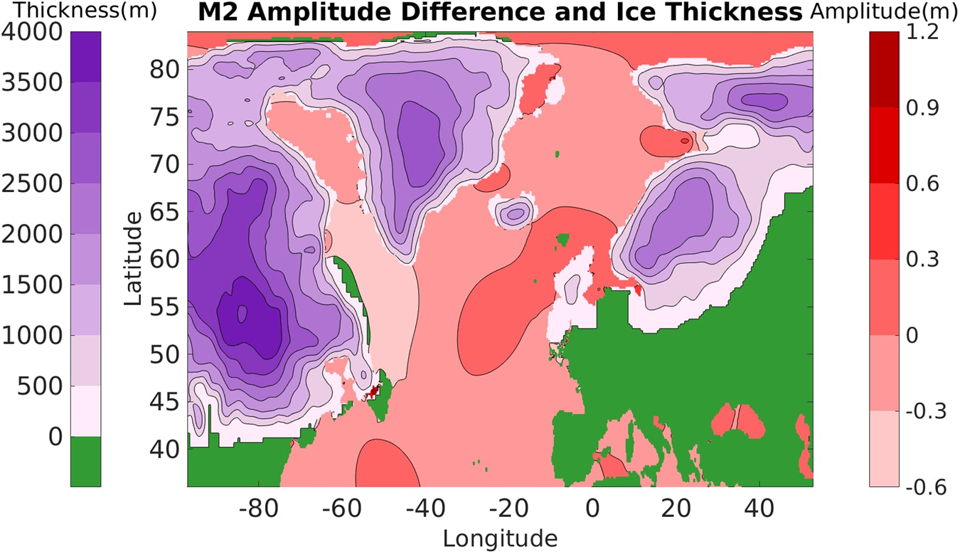
An important additional result of the analysis presented by Velay-Vitow et al. (Reference Velay-Vitow, Peltier and Stuhne2020) was that the removal of the ice grounded in Hudson Strait had a significant effect on the state of the North Atlantic resonance of the M2 tidal constituent as shown in Figure 3, in which we show the difference between the amplitude of the M2 tide before and after instability occurrence. If it is imagined that an altogether different ice stream located in the ice-covered continental region of the eastern sector of the North Atlantic was responsible for anomalous HEs, as was suggested in Hemming (Reference Hemming2004), it would be helpful to identify candidate ice streams and to consider whether or not they might be susceptible to the same instability mechanism as the one we have shown to be highly plausible for the majority of H-events. If it were found to be the case that eastern-sector instabilities were highly plausible, this would undermine the plausibility of our suggested mechanism for H-event recurrence time. Our goal in this paper is to provide detailed examinations of several candidate ice streams and to comment on the question as to whether they should be viewed as plausible possibilities for the explanation of anomalous H-events.
In our model, the effect of H1 on the resonant state of the M2 tide in the North Atlantic was particularly profound outboard of the Hudson Strait, with a drop in tidal amplitude of between 0.3 and 0.6 m. Figure and caption adapted from Velay-Vitow et al. (Reference Velay-Vitow, Peltier and Stuhne2020).

Candidate models for Heinrich event 3
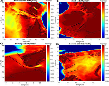
In modeling H3, the initiation and duration of the instability and the extent of the deglaciation must be determined. We make use of the results in Hemming (Reference Hemming2004) in the design of a plausible model and choose 31 ka as an initiation time for the (assumed to be related) ice stream instability and 1200 years as the duration of the model event. The duration of the modeled event was determined by averaging the three different estimates for the duration of H3 listed in table 3 of Hemming (Reference Hemming2004). To determine the plausible regions of ice stream instability that might have been the source of a non-Hudson Strait H3 event, we first examined the crustal depression predicted at each of the most plausible candidate locations by the ICE-7G NA (VM7) model of Roy and Peltier (Reference Roy and Peltier2017, Reference Roy and Peltier2018) to search for similar features to those of the Hudson Strait reported by Velay-Vitow et al. (Reference Velay-Vitow, Peltier and Stuhne2020). Specifically, we search for regions in which the nature of the crustal depression beneath grounded ice cover is such that the depression increases with distance “up ice” from the point at which grounded ice cover abuts the Atlantic Ocean. The nature of the crustal depression beneath grounded ice in the ICE-7G NA (VM7) model of Roy and Peltier (Reference Roy and Peltier2017, Reference Roy and Peltier2018) for each of our candidate locations is presented in Figure 4. Panel A of the figure illustrates the depth of the crustal depression in Hudson Strait, and the remaining panels of the figure show the same data for our three eastern North Atlantic candidate ice streams. This characteristic of the crustal depression beneath an ice stream has been demonstrated by Schoof (Reference Schoof2007, Reference Schoof2012) to be the most important requirement for an ice stream to be susceptible to instability when the grounding line is subjected to a sufficiently intense buoyancy forcing to move it downslope. In all three of the eastern North Atlantic candidate ice streams, the crustal depression along the bed of the proposed ice stream is smaller in magnitude than that observed in the Hudson Strait case, suggesting that the requirement for instability will be more difficult to meet in these regions.
The crustal depression under the weight of terrestrial ice sheets at each of the three candidate eastern North Atlantic locations, as well as the Hudson Strait, immediately before the onset of H3 at 31 ka is presented. In panel A), the crust underlying the Hudson Strait has qualitative features that are nearly identical to those identified by Velay-Vitow et al. (Reference Velay-Vitow, Peltier and Stuhne2020). The Irish Sea crustal depression in panel B) shows only a slight inland deepening, while the Norwegian ice stream, presented in panel C), shows a clear increase in depth in the up-strait direction. As shown in panel D), the center of the Barents Sea is depressed relative to the edges, and the depth increases from west to east. Furthermore, there is a local maxima of depth separating the North Atlantic Ocean from the Barents Sea. All three candidate locations have features somewhat similar to those observed in the Hudson Strait. The black bars indicate the approximate location of candidate ice streams.

Velay-Vitow et al. (Reference Velay-Vitow, Peltier and Stuhne2020) suggested that the forcing of the ice stream at its point of contact with the ocean, which was needed to induce instability, might have been provided by anomalously high tides, a condition that was extremely well satisfied by the conditions of the Hudson Strait ice stream prior to H1. These conditions are qualitatively similar to the conditions in the Hudson Strait prior to H3 (see Figure 4). If similar features were found to exist at one or more of our eastern Atlantic candidate locations, this would allow the same model employed in the H1 analysis to be applied to these additional candidate ice streams. In addition to the three locations on the east coast of the North Atlantic, the Hudson Strait ice stream was also examined. In each case, H3 was modeled by modifying the ICE-7G NA (VM7) model of ice-loading history from Roy and Peltier (Reference Roy and Peltier2017, Reference Roy and Peltier2018) to determine the paleobathymetric depth that would exist once the grounded ice was eliminated from the region assumed to have been filled by the candidate ice stream; this depth is then used as an input to the shallow-water tidal solver. Although this model includes no ice dynamical processes, such as calving, the grids generated for the tidal solver only depend on whether a given cell is ocean or land. The additional sea-level rise associated with realistic ice stream dynamics is assumed to be negligible and is therefore ignored.
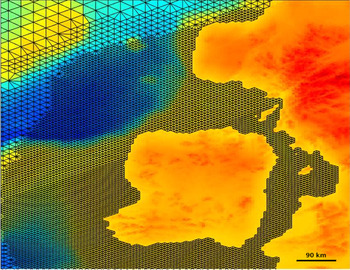
As in Velay-Vitow et al. (Reference Velay-Vitow, Peltier and Stuhne2020), we make use of a non-uniform grid that is more highly resolved in each of the proposed locations, as well as in the region of high resonance in the Labrador Sea, to accurately model the effect deglaciating the proposed ice streams has on the tidal regime in the North Atlantic. The grids we employ have a maximum internodal spacing of 30 km in the open ocean, and a minimum of 7.5 km near the coasts. The grid used for the Ireland case is presented in Figure 5.
(color online) The globally unstructured grid is locally refined in the vicinity of the hypothesized ice stream in the Irish Sea. In the upper left of the figure, the transition region from comparatively higher internodal spacing of 30 km to the lower spacing of 7.5 km is seen.

RESULTS AND DISCUSSION
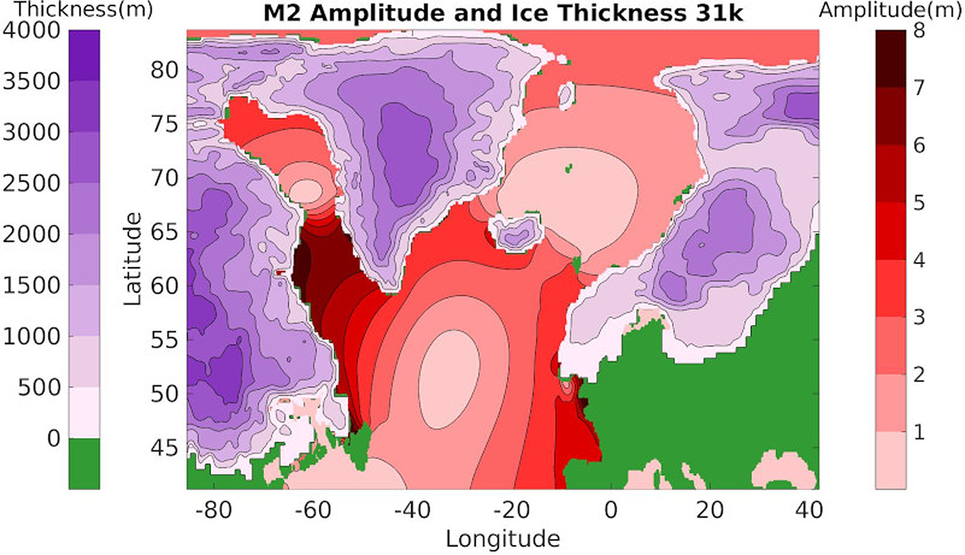
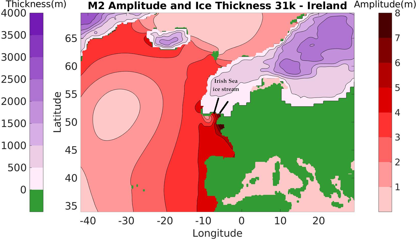
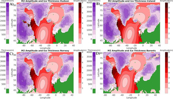
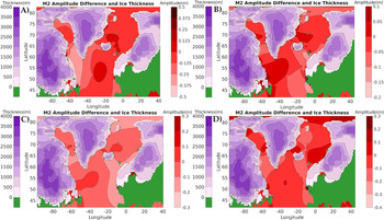
The M2 tidal constituent was modeled for each of the three eastern North Atlantic locations, as well as for the Hudson Strait, at 29.8 ka, which is the time assumed to be coincident with the time of termination of the H3 instability. In Figure 6, the M2 tidal constituent is shown for the North Atlantic at 31 ka, and in Figure 7 the area of the North Atlantic directly south of the Irish Sea is shown. The ice thickness and M2 tidal amplitude are shown in each of the four cases in Figure 8, and the change in tidal amplitude from 31 ka to 29.8 ka is shown for each case in Figure 9. The kinetic and potential energy of the global ocean both prior to and after H3 is presented for each modeled case in Table 1.
(color online) The M2 tidal constituent and ice thickness are presented at 31 ka, as calculated by the discontinuous Galerkin model. The tide is in a state of resonance at 31 ka, with the point of highest amplitude in the Labrador Sea, immediately out board of the Hudson Strait.

(color online) The M2 tidal constituent and ice thickness is presented for the portion of the North Atlantic Ocean directly south of the Irish Sea. This location experiences a 5–6 m amplitude M2 tide prior to a proposed deglaciation of the Irish Sea ice stream.

The M2 tidal constituent is presented at the end of H3, 29.8 ka. In all four cases examined, the tidal regime in the North Atlantic looks very similar. The case where the Hudson Strait was assumed to deglaciate is shown in panel A). The Hudson Strait itself is megatidal, with tidal amplitudes as large as 8 m. In panel B), we see that the deglaciation of the Irish Sea ice stream has resulted in 4–5m amplitude tides in the Irish Sea. In panels C) and D), which show the cases where the Norwegian ice stream and Barents Sea were assumed to deglaciate, respectively, these regions are seen to be micro tidal, with M2 tides less than 1 m in amplitude.

By examining the differences between each case and the M2 tide at 31 ka, the effects of each of the cases on tidal amplitude can be seen more clearly. In panel A), where the Hudson Strait is assumed to deglaciate, the North Atlantic experiences a decrease in tidal amplitude of between 0.25 and 0.5 m, and this decrease is concentrated on the North American coast. In panel B), where the Irish Sea is assumed to deglaciate, the M2 tide is largely unaffected, except in the local vicinity. In panel C), where the Norwegian ice stream is assumed to deglaciate, we see a decrease in tidal amplitude of between 0.1 and 0.2 m over the North Atlantic. Panel D), where the Barents Sea was assumed to deglaciate, shows a decrease in the tidal amplitude of between 0.2 and 0.3 m in the North Atlantic.

An eastern-sector North Atlantic ice stream that significantly affected the North Atlantic M2 tidal resonance upon deglaciation could hypothetically explain the anomalous nature of H3, as a decrease in the strength of the M2 tide could potentially lead to a weaker tidal forcing of the Hudson Strait ice stream. However, in all three candidate cases, the effect of an ice stream deglaciation on the North Atlantic tidal regime is similar qualitatively, but the magnitude of the effect is quite small. The North Atlantic M2 tidal resonance decreased the most directly outboard of the Hudson Strait in all cases, with the exception of the control case where deglaciation was assumed to occur in the Hudson Strait itself. This effect, although small, is a reasonable feature of the model as the area immediately outboard of the Hudson Strait has the highest amplitude M2 tide in the North Atlantic prior to H3. Furthermore, each of the four cases results in a slightly weaker North Atlantic resonance in general. In the case where the Hudson Strait is assumed to deglaciate, the area immediately outboard of the entrance to the strait experienced a slight increase in M2 tidal amplitude, likely due to the increased tidal amplitude in Ungava Bay. In the case of the Barents Sea ice stream and Norwegian ice stream, the tidal amplitude within the portion of the ocean exposed by deglaciation is quite small. However, in the case of the Irish Sea ice stream, there is a 4–5-m amplitude M2 tide after deglaciation, implying a tidal range of 8–10 m.
Each of the three eastern Atlantic locations had some similar properties to the Hudson Strait, although there are notable differences described below, and in no location did deglaciation significantly influence the resonant state of the M2 tide in the North Atlantic. It can be surmised on a priori grounds, based on the differing “sharpness” of the occurrence of a retrograde slope in the up strait direction, that this might be the case. This is to say that there is an extended portion of the proposed strait that is relatively flat, prior to the region of significant retrograde slope.
Neither the Norwegian ice stream nor the proposed Barents Sea ice stream was close enough to the region of enhanced tidal resonance in the North Atlantic to have a significant influence. The Irish Sea ice stream, although immediately adjacent to the North Atlantic, did not have a significant effect on the resonant state of the M2 tidal resonance when it was assumed to deglaciate. This is likely due to the Irish Sea ice stream being much more localized than the ice stream that existed in the Hudson Strait. Accordingly, it is reasonable that the effect on the resonance would be weaker. None of the examined locations had all the properties required to support a strong argument in favor of a tidally triggered marine ice stream instability. In the case of the Barents Sea, the proposed deglaciation was imagined to occur in a large, shallow depression as opposed to a single deep channel. The Norwegian ice stream was located in a single deep channel, but the entrance to the channel is quite broad, and the slope of the crust underlying the paleo ice stream is too shallow for rapid deglaciation to occur. Finally, in the case of the Irish Sea ice stream, despite being a site of large amplitude tides prior to H3, this region possesses an insignificant increase in crustal depression along the extent of the proposed ice stream, which allows us to infer that a marine ice stream instability is unlikely, though not entirely ruled out as a possibility. As such, we conclude that the Hudson Strait is the most likely source of the ice stream instability associated with H3. This conclusion is in agreement with Andrews and Voelker (Reference Andrews and Voelker2018) and requires a different explanation for the anomalous nature of the sediment signature associated with H3 in North Atlantic sediment cores.
Returning to the five differences between LHEs and anomalous HEs noted by Gwiazda et al. (Reference Gwiazda, Hemming and Broecker1996a), we suggest that the first difference, the more gradual onset of H3, is partially responsible for the other differences. We also propose that the relatively extended duration of H3 may help provide an explanation for the reduced presence of IRD, compared to LHEs. As H3 was an event that began gradually and persisted over a duration at least twice as long as that of H1, it is possible it was a less violent event, where the instability propagated less rapidly in the inland direction. As the ice eliminated from the ice stream by the instability would have had an extended opportunity to melt in the Hudson Strait due to the slower progression of the instability, the freshwater forcing to the North Atlantic could have been composed of a higher ratio of meltwater to icebergs than other H-events. This could potentially explain the noted anomaly in the IRD ratio, via two mechanisms. The ice that is eventually transported to the North Atlantic could have already redeposited a significant fraction of its entrapped sediment onto the floor of the Hudson Strait due to longer residence time, and the meltwater forcing could have produced the decrease in forams noted in the sediment column. Additionally, a less violent event may have scraped a smaller amount of lithic fragments from the sidewalls and floor of the strait, which would have created an IRD signature that contained less detrital carbonate. That the source of the sediments associated with H3 in cores recovered from the eastern North Atlantic is dissimilar to that of other H-events is plausibly explained by a smaller fraction of the icebergs persisting that far east while still containing sediment. Note, however, that our model does not provide a completely satisfactory explanation for the observed difference in the Sr and Nd isotopic analysis of the silicate fraction along the Ruddiman belt.
Two questions remain: Why did H3 have a more gradual beginning, and why did it occur over a longer duration of time? Answering these questions could resolve the issue of the anomalous nature of H3. The work presented here generates a few observations relevant to this issue:
• The M2 tidal amplitude immediately prior to H3 is similar to that prior to H1
• H3 occurred at 31 ka during a period of exceptionally cold glacial conditions
• The distribution and thickness of the ice over the Hudson Strait is unlikely to have been the same for all H-events
As H1 had a duration of approximately 500 years, it is unlikely that the difference in duration between it and H3 was due to weaker tidal forcing, as there is no evidence that this was the case. However, the colder atmospheric conditions and the possibility of varying ice thicknesses are more promising as potential explanations for the anomalous nature of H3. If the ice over the Hudson Strait was thinner prior to H3 than it was prior to H1, it is expected that the slope of the underlying bed may have been less extreme. This, coupled with the colder climatic conditions, might have slowed the propagation of the instability or perhaps slowed the rate at which ice flowed from the Laurentide Ice Sheet into the cleared strait after the instability occurred.
Although the tidal triggering mechanism does not appear to have been active in eastern-sector ice streams during H3, ongoing work in other geographical regions indicates this mechanism was almost certainly active during deglaciation of the Laurentide Ice Sheet along the coast of the Arctic Ocean where Griffiths and Peltier (Reference Griffiths and Peltier2008, Reference Griffiths and Peltier2009) have shown that the tidal regime under glacial conditions was characterized by high-amplitude tides, whereas under modern conditions the tides are extremely weak. The same may be the case for Antarctica where the same authors have suggested that strong tides were also quite likely at the peak of glaciation, whereas they are also weak in the modern ocean. We are therefore suggesting that tidal destabilization of marine-terminating ice streams may have played a significant role in the transition from glacial to interglacial conditions.
CONCLUSION
We have shown that none of the candidate ice streams in the eastern sector of the North Atlantic are likely to have been rendered unstable by a high amplitude M2 tide at the time of H3, though of the three cases presented, the Irish Sea ice stream is the most likely candidate. We tentatively conclude that tidally forced ice stream instability is a plausible explanation for H-events only in the case of Hudson Strait. In the present paper, we have further proposed that most of the sedimentological anomalies associated with H3 can be potentially explained by the longer duration of H3 and that eastern-sector ice streams need not necessarily be invoked in any case. Our results are in agreement with recent literature that suggests all H-events can be traced to an instability in the Hudson Strait ice stream. It appears therefore that the main source of the ice involved in H3 is the Hudson strait, although more work will be required to better understand, in the context of this tentative conclusion, the reason the H3 instability evolved more gradually and continued over a longer period of time. One possibility in this regard is that the steepness of the depression of the crust beneath the ice stream that existed in Hudson Strait was somewhat reduced at the time of the onset of the H3 instability in comparison with the majority of the H-events that occurred during MIS 3.
ACKNOWLEDGMENTS
The funding support to Jesse Velay-Vitow from the University of Toronto Department of Physics, as well as the Cray Corporation, has been greatly appreciated. All of the computations performed in the context of this work made use of the SciNet facility of the University of Toronto, which is a component of the Compute Canada platform for High Performance Computation. The research of WRP in Toronto is supported by Natural Sciences and Engineering Research Council Discovery Grant A9627.
The paleo-crustal and ice thickness datasets used in the analyses presented can be retrieved from the website of WRP and can be found at http://www.atmosp.physics.utoronto.ca/peltier/data.php.