1 Introduction
In recent years, there has been increasing interest among both economists and policy makers in the possible consequences of population ageing, and in particular on how to make social security systems more sustainable in light of this. The adequacy of pension systems has been largely called into question, and a number of works show that there are strong implicit and explicit incentives to leave the labour market embedded in the pension systems of most developed economies.
Italy may be included amongst the countries where retirement behaviour is stretching most the sustainability of the social security system. D'Addio et al. (Reference D'Addio, Keese and Whitehouse2010), for example, show that in Organisation for Economic Co-operation and Development (OECD) countries older workers (50–64) are less likely to be in employment than their prime-aged counterparts (aged 25–50), with high cross-country variability. At one extreme, there are countries like Japan and USA where older participation rates are over 70%; at the other extreme, there are countries, including Italy, where older participation rate is below 50%.
Besides, in most OECD countries workers tend to leave the labour market before the pensionable age. Italy was the country with the lowest pensionable age for workers who retired in 2006 (57 years) and one of the countries with the lowest average effective age of labour-market exit in the period 2002–07 (60 years) (D'Addio et al., Reference D'Addio, Keese and Whitehouse2010). This also implies a huge proportion of unused labour capacity of older workers, with Italy again appearing among the countries where this proportion is highestFootnote 1 (Gruber and Wise, Reference Gruber and Wise1998; Börsch-Supan et al., Reference Börsch-Supan, Brugiavini, Jürges, Mackenbach, Siegrist and Weber2005). These challenges have been tackled in Italy, starting from the nineties, through several major reforms as well as minor adjustments to the social security system, with the main aim of increasing its financial sustainability.
There is now plenty of evidence explaining these retirement patterns and describing the incentives to leave the labour market embedded in the pension system. Researchers who have recently examined cross-national differences in pension incentives generally find they have predictable and significant effects on labour force withdrawal: countries with early pension ages, generous income replacement and heavy implicit taxes on earnings in old age tend to have earlier exit from the labour force than countries with pension systems that provide fewer work disincentives (Gruber and Wise, Reference Gruber and Wise1999; Burtless, Reference Burtless2004).
Many of the studies that try to uncover the relationship between incentives and retirement may be included in the literature of the reduced form of the option-value model. This model aims at capturing the forward-looking behaviour of individuals by comparing the value of retiring today with the value of retiring at any future date. Results in this literature seem to suggest sizeable effects of social security incentives on retirement.Footnote 2 However, results are not so clear-cut for all countries,Footnote 3 and in general, this literature struggles in disentangling the effect of social security from individuals’ preferences heterogeneity, especially when there is not sufficient exogenous variation in social security rules.
A more restricted strand of literature exists that looks instead at specific reforms of the pension or social security system and uses policy evaluation strategies to identify their causal effect on retirement decisions. The advantage with respect to the option-value literature is that the effect of interest is more reliably identified by an exogenous variation of the incentives, which makes the causal interpretation of results more convincing.
Krueger and Pischke (Reference Krueger and Pischke1992) study the 1977 amendments to the Social Security Act in the USA, which led to a downward change in social security benefits for one generation of workers while leaving benefits unchanged for previous generations. Pencavel (Reference Pencavel2001) investigates severance pay in the employee buyout program implemented by the University of California in the early 1990s,Footnote 4 which offered additional pension benefits to those older faculty who agreed to retire by a certain date. Mastrobuoni (Reference Mastrobuoni2009) studies the reduction in Social Security benefits due to an increase in the Normal Retirement Age in the USA at the beginning of the 1980s. Hanel and Riphahn (Reference Hanel and Riphahn2012) study a Swiss pension reform and Atalay and Barrett (Reference Atalay and Barrett2015) investigate the 1993 Australian Age Pension reform, which both increased eligibility age for women. All of these studies, with the exception of Krueger and Pischke (Reference Krueger and Pischke1992), find significant individuals’ responses to the reforms in the expected direction.
While this paper fits into this second strand of the literature, it studies a reform characterized by unique features. The so-called ‘super-bonus’ reform was implemented in Italy between 2004 and 2007 and consisted in the possibility for workers in the private sector eligible to early retirement to continue working without paying social security contributions. The proclaimed intent of the reform was to induce these workers to delay retirement in order to mitigate the sustainability problems of the social security system, but it did not provide a straightforward positive incentive to do that. The reason for this is that, by not paying social security contributions, any additional time spent working while receiving the bonus did not contribute to increasing future pension benefits.
While previous studies have evaluated policies that decreased (increased) the generosity of pensions, thus having the clear expected effect of increasing (decreasing) age of retirement, the super-bonus reform has an a priori unclear effect on individuals’ behavior. On the one hand, it will be shown that, when taking into account all the financial consequences of taking up the bonus, the reform provides a negative incentive to delay retirement for most workers. On the other hand, the reform gave the unique chance of increasing one's income today in exchange for lower pension benefits in the future. This can be interpreted as an opportunity of borrowing against future social security benefits, which is normally not allowed by the Italian legislation.
As the reform was directed to private sector workers only, it provides a quasi-natural experiment setting where public workers’ retirement behaviour can be used as counterfactual. A difference-in-differences (DID) strategy will allow to interpret the results causally. Besides the usual linear probability model (LPM), a new approach to DID estimation in probit models, proposed by Blundell et al. (Reference Blundell, Dias, Meghir and Reenen2004), will be exploited as a robustness check of results. This approach accounts for the fact that the marginal effects on interaction terms in non-linear models, differently from linear models, cannot be interpreted as a DID estimator.
Results suggest a reduction of 7 ppt (or 30%) in the proportion of private workers who decided to retire among those qualifying for retirement, despite the fact that the incentive was negative for most workers. The robustness of results is checked against the use of different models and specifications. When investigating heterogeneity in the response, DID results suggest that the effect of the reform is driven by low-income workers (11–14 ppt reduction, depending on the model used). Even if it is not possible to give a straightforward explanation of these results, it is argued through some empirical evidence that liquidity constraints and financial (il)literacy may help to interpret them. Low-income individuals may want to take advantage of the opportunity of borrowing against future pension benefits, given that they are more likely than high-income individuals to be liquidity constrained. At the same time, however, it cannot be excluded that low-income individuals, who are shown to be more likely financially illiterate, did not fully internalize the consequences of the reform. Either explanation, or both, are compatible with the observed results.
The structure of the paper is as follows. Section 2 describes the Italian institutional setting and the characteristics of the ‘super-bonus’ reform. Section 3 introduces the data and provide some descriptive statistics on retirement in Italy and on the characteristics of the sample of workers. Section 4 describes the estimation strategy and presents the first results. In Section 5, a discussion and interpretation of results is provided. Section 6 concludes.
2 The ‘super-bonus’ reform
Italy underwent three major reforms of the pension system in the nineties, with the aim of increasing the financial sustainability of the system.Footnote 5 The main features of the reforms were an increase in the retirement age and minimum years of contributions for pension eligibility, a gradual shift from a defined benefit system towards a contribution-based system, indexation of pension benefits to prices rather than to wages and the introduction of complementary social security. Besides, they abolished seniority retirement for all those who started working after 1995. Seniority retirement is a form of early retirement which allowed to retire before the old-age retirement age without adjustments of the pension benefits. The only requirement was to possess either both a minimum number of contributions years and a minimum age or only a (higher) minimum number of contribution years, independently from age.
The above mentioned major reforms were followed by other minor measures up until the Maroni reform of 2004. The aim of this reform was twofold: first of all, increasing the retirement age, mainly on a voluntary basis, and second the development of complementary social security next to the usual public social security system. It provided also for further increases in pensionable age and contribution requirements and was partly modified in 2007.Footnote 6
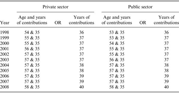
The focus of this study will be on the evaluation of the effects on retirement decisions of the so-called ‘super-bonus’, which was indeed part of the 2004 reform. The bonus consisted in economic incentives directed to private sector workers who had reached seniority pension requirements in between October 2004 and the end of 2007 (but who had not reached requirements for old age pension yet) and who chose to delay retirement despite having reached eligibility. Crucially for this study, public workers were not entitled to the bonus. The age and contribution requirements in the reform years were similar for public and private workers and the same for men and women and as mentioned above, amounted to either both an age and contribution requirement or only a (higher) contribution requirement (see Table A1 for details). Old age eligibility was 65 years for men and 60 years for women for both public and private workers. The effects of the bonus ceased when the worker decided to retire, by reaching old age pension requirements or by the end of 2007. After this date, the worker could decide to continue working with no incentives, thus going back to the pre-bonus compensation net of social security contributions.
The amount of the incentive to postpone retirement corresponded to the social security contributions that employers and employeesFootnote 7 normally pay to the social security system, which amounted to 32.70% of gross salary for most workers (33.70% on earnings above 37,884 Euro). The amount of the incentive relative to gross income was thus the same for everyone.
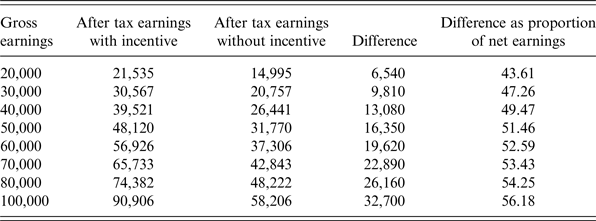
However, as the extra salary was untaxed and due to the progressivity of labour income taxes, the percentage increase with respect to net earnings was even bigger than the nominal contributions value, as it was increasing more than proportionally with net earnings. An example will help visualizing the implications of the incentive on earnings (see Table 1): a worker earning a gross yearly salary of 20,000 Euro would earn a net salary of 14,995 Euro with no incentive and of 21,535 Euro with the incentive, while at the other extreme one individual earning a gross salary of 100,000 Euro would earn 58,206 Euro with no incentive and 90,906 Euro with the incentive, meaning that for this individual the increase exceeded 56% of the net salary, versus a 43.61% increase for the former worker.
The effect of the super-bonus on earnings

Notes: Author's calculations based on hypothetical earnings and 2004 tax rules.
As the worker was not paying contributions during the bonus period, the pension she was entitled to remain fixed at the level accrued at the moment she joined the super-bonus. Besides, it should be also taken into account that every working year with no bonus determines a pension increase equal to 2% of the last working years average salary, a percentage that progressively decreases to 0.90% for salaries above the 37,884 Euro pensionable limit. This is an additional reason making the incentive more convenient for high-income workers. It should be clear at this point that understanding the ‘true’ amount of the incentive is a non-straightforward task which involves a trade-off between a higher current salary and fixed future benefits.
In the spirit of Manoli and Weber (Reference Manoli and Weber2016), the change in monetary incentives can be calculated by comparing the financial incentives to retire in presence of the bonus to the incentives (embedded in the social security system) in absence of the bonus.
In a dynamic framework, workers in each period evaluate the choice between continue working and retire by comparing current and future benefits from these two choices. For this reason, the incentive measure should be a forward-looking measure that takes into account the trade-off between labour income and changes in social security wealth, net of taxes and benefits. This is the approach used, for example, in the reduced-form literature on retirement decision (see, among others, Gruber and Wise (Reference Gruber and Wise2004)).
As in Manoli and Weber (Reference Manoli and Weber2016), the incentive of retiring is measured using the concept of ‘implicit tax rate’ on gross annual earnings τ, where τ is defined such that after-tax income (left-hand side of (1)) is equated to gross earnings net of all taxes and retirement benefits (right-hand side of (1)):
 $$(1 - \tau )y = y(1 - \tau _{SS})(1 - \tau _E) - b(1 - \tau _b) + \Delta SSW$$
where (1 − τ) is commonly called ‘net-of-tax rate’. τ SS and τ E denotes social security contribution and income taxes respectively. b and τ b denotes annual pension benefits and taxes on pension benefits respectively; benefits enter negatively as they represent foregone income from postponing retirement. SSW denotes social security wealth, defined as the expected present discounted value at age a of benefits received from retirement age R:
 $$SSW_{a,R} = \sum\limits_{s = R + 1}^\Omega \beta ^{s - a}\pi (s \vert a)b_R(s)$$
where Ω is the maximum survival age (assumed here to be 110 years), β is the discount factor (=0.97, corresponding to a 3% discount rate) and π(s|a) is the survival probability (by gender) conditional to age a.Footnote 8 ΔSSW in Equation (1) denotes the change in social security wealth from postponing retirement of 1 year (from R = a to R = a + 1), that is: SSW a,a+1 − SSW a,a. This corresponds to the concept of ‘accrual’ commonly used in retirement literature, which enters positively as a positive ΔSSW indicates an incentive to delay retirement, while a negative ΔSSW indicates a disincentive.
Given that the super-bonus reform consisted in the suspension of due contributions, the implicit tax rate on gross earnings with the bonus is given by τ bonus such that:
 $$(1 - \tau _{bonus})y = y(1 - \tau _{SS})(1 - \tau _E) + y\tau _{SS} - b(1 - \tau _b) + \Delta SSW_{bonus}$$
It should also be noticed that ΔSSW bonus is different from ΔSSW. The decision of postponing retirement, in fact, entails two effects: the first one comes from the pension rules and normally implies an increase of the pension benefits due to the increased social security contributions. The second effect on SSW is due to the shorter retirement period, and it is thus negative. As with the bonus, benefits were kept fixed at the pre-reform level, the change in SSW with the bonus is only due to the shorter retirement period and, thus, can only be negative.
The change in the net-of-tax rate would then be a measure of the change in the incentive to postpone retirement of 1 year in the two scenarios, with and without bonus. It may be written as:
 $$\Delta (1 - \tau )y = [(1 - \tau _{bonus}) - (1 - \tau )]y = y\tau _{SS} + \Delta SSW_{bonus} - \Delta SSW$$
which makes clear that the change in the net-of-tax rate could be either a positive or negative number. Here this value represents the change in the incentive of postponing retirement from the end of 2004 (when the reform was implemented) to the following year, for the private sector workers eligible to retire.Footnote 9, Footnote 10
The average implicit tax rate τ that is estimated in the normal case (i.e., without bonus) amounts to 0.55, meaning that there is a huge disincentive to postpone retirement of 1 year: on average, more than half of any extra Euro earned when postponing retirement would be lost. With the bonus, the average implicit tax rate amounts to 0.84, meaning that the reform actually provided a (bigger) disincentive to retire.
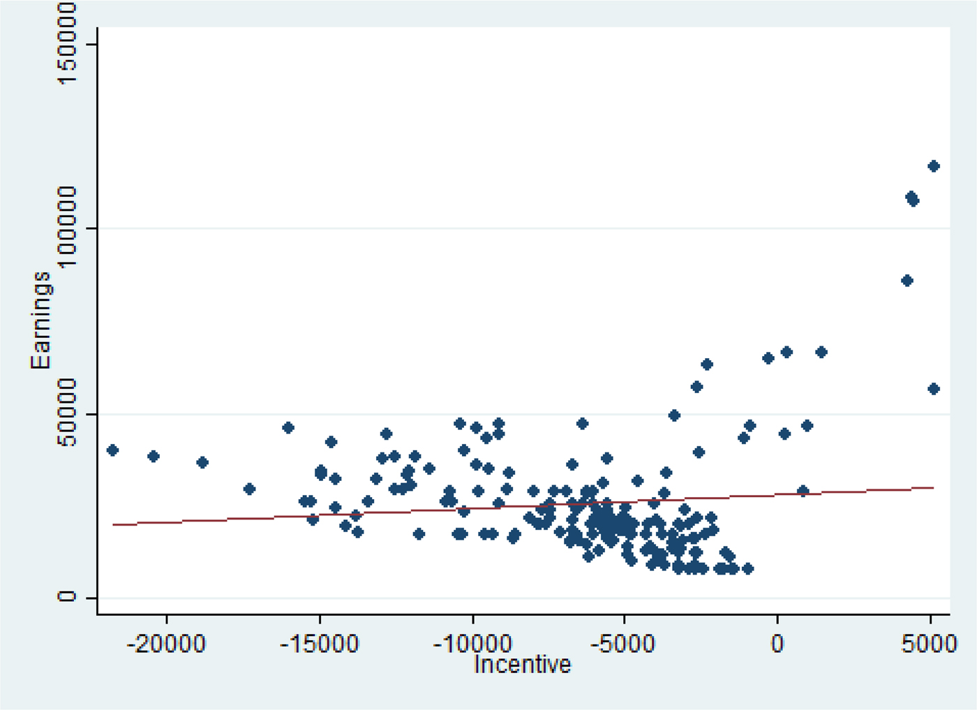
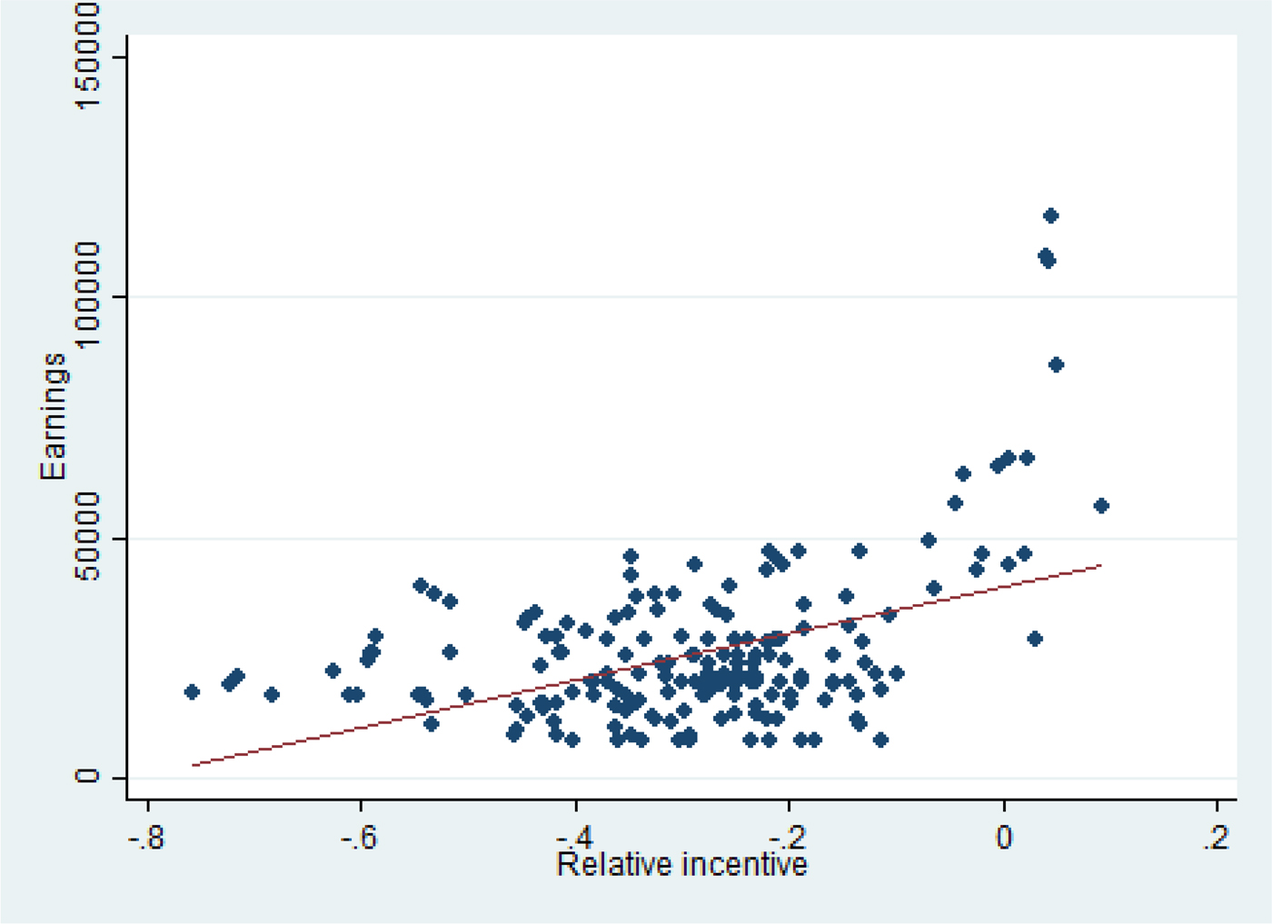
In Figures 1 and 2, the relationship between earnings and the bonus is depicted: in the former, the bonus is measured in absolute terms (as in Equation (4)), in the latter it is measured relative to earnings. The graphs show that the bonus increases with earnings, both in absolute and in relative terms, but slightly so. The reason is that the majority of workers in the sample falls into the lowest tax brackets and below the pensionable limit. More interestingly, they also show that the bonus is actually negative for the vast majority of workers.
Monetary incentives by earnings. Notes: This figure shows the relationship between the imputed incentive (x-axis) and gross labour income (y-axis) for private workers in the first reform year. The incentive is calculated based on 2004 tax and pension rules. The sample is drawn from the 2004 SHIW. Monetary values in Euro 2010.

Relative monetary incentives by earnings. Notes: This figure shows the relationship between the imputed relative (to gross income) incentive (x-axis) and gross labour income (y-axis) for private workers in the first reform year. The incentive is calculated based on 2004 tax and pension rules. The sample is drawn from the 2004 SHIW. Monetary values in Euro 2010.

It should be made clear that the aim of this exercise is not to provide a precise evaluation of the actual individual gain or loss from taking up the bonus. In fact, it is not possible to know who exactly took up the bonus and for how long. Rather, two main messages are delivered, which will be important in the remaining of the paper. First, the bonus provides a disincentive to retire which decreases with earnings; second, a rather complicated calculation is necessary to fully understand the monetary implications of the reform.
3 Data and descriptive analysis
The data used to investigate the effects of the super-bonus on retirement decisions are taken from the Bank of Italy Survey on Household Income and Wealth (SHIW). The SHIW started in the 1960s, with interviews conducted approximately every 2 years, and microdata are available starting from the 1977 survey. Up to 1987, the survey was conducted with time-independent samples (cross sections) of households but since 1989 part of the sample has comprised also households interviewed in previous surveys (panel households). Nevertheless, cross-sectional data will be used in this analysis for the sake of sample size. The questionnaire focuses on perceived well-being, the situation of the household of origin, payment instruments and financial information. It includes various pieces of information useful for the analysis of the super-bonus, especially the possibility to distinguish between public and private workers and the number of contribution years.
In the empirical analysis, data from 2002 to 2008 will be exploited,Footnote 11 as the interest is in comparing retirement behaviour during reform years and in pre-reform years. As said above, the reform took place in between October 2004 and the very end of 2007. However, because of the peculiar exit mechanism in place, once individuals formally apply for retirement, reform and pre-reform years need to be redefined. In particular, individuals who reached pension requirements and ask to retire in a given quarter of the year have then to wait for the first ‘exit window’ to actually retire. This window falls two quarters after the time of the retirement request, thus the individuals who are seen retiring in 2005 are individuals who became eligible at the end of 2004 or earlier, and individuals who joined the reform up until the end of 2007 could retire only in 2008.Footnote 12 For this reason, pooled data from 2002 and 2004 surveys will provide information on pre-reform behaviour, while data gathered from the 2006 and 2008 surveys will inform on individuals’ behaviour during the reform period.
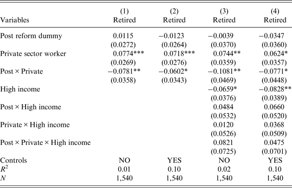
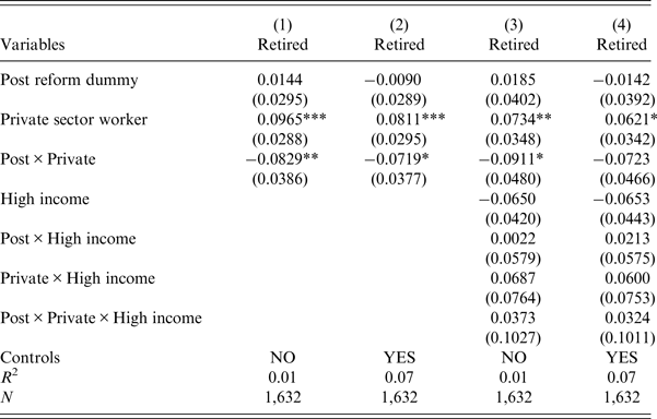
The sample will be composed of individuals who reached the age and contributions requirements necessary for seniority pension, and the outcome of interest will be the percentage of these individuals retiring each year. These individuals can be identified because the dataset contains information on contribution years and on the year when retired individuals started drawing their pension. In the main analysis, also individuals who had reached the contribution requirements but not the age requirements for seniority pension will be included. The reason is twofold: first, very specific eligibility rules apply to many minor categories of workers, which cannot be clearly identified given the information contained in the survey.Footnote 13 As special rules are always more generous than the general ones, using this sample definition guarantees that workers who are actually eligible are not excluded from the sample. Second, even if some of these individuals are not currently eligible, they will become eligible in later reform years.Footnote 14 As the reform is less salient for these individuals, a robustness check will be performed using a reduced sample which excludes them.
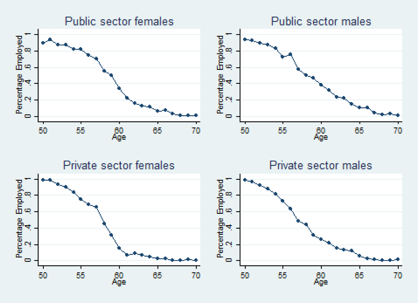
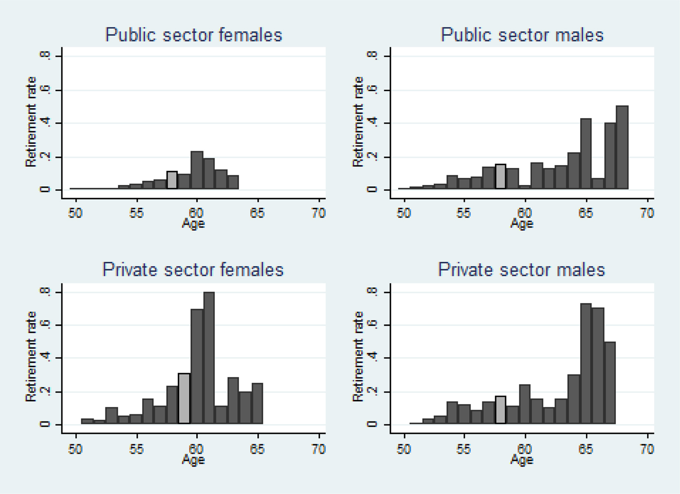
Figure 3 shows employment frequencies averaged over pre-reform years (1998–2004), separately for males and females and for public and private workers. It is apparent from this figure that employment decreases fast at all ages, and it is possible also to notice a clear tendency towards retirement before old age (60 years for women and 65 years for men). The average age of retirement was 58 years for women and 59 for men. Figure 4 shows instead the hazard rate by age,Footnote 15 separately for males and females. Red bars represent the median age of retirement, which are again below old age eligibility. This figure clearly shows the presence of spikes in retirement percentages at specific ages, which usually correspond to eligibility ages.Footnote 16
Employment frequencies by sector and gender, 1998–2004. Notes: Author's calculations based on SHIW data. Each dot represents the ratio of the employed to the non-unemployed working age individuals at a specific age, by gender and sector of employment. Averages over years 1998–2004.

Hazard rates of retirement by sector and gender, 1998–2004. Notes: Author's calculations based on SHIW data. Each bar represents the percentage of individuals that retire at a specific age conditional on not being retired at any prior age, by gender and sector of employment. Light gray bars represent sample medians. Averages over years 1998–2004.

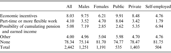
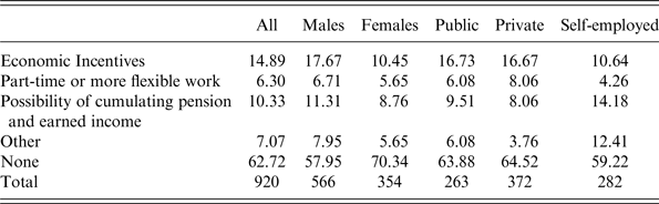
In Tables 2 and 3 the results of two questions that appeared only in 2002 survey are shown. Specifically, the questions asked to those who retired before maximum retirement age (Table 2) and to those expecting to retire before maximum pensionable age (Table 3) if they would have worked longer, or would work longer, under certain conditions. These comprise economic incentives, part-time or more flexible work and the possibility of cumulating pension and earned income. Results are also split by sex and work sector (public, private or self-employed). The percentage of retired who claim they would not have worked longer is higher than the same percentage among workers who expect to retire early. However, for both categories, economic incentives seem to be the most appealing condition for postponing retirement, followed by the possibility of cumulating pension and earned income and by part-time or more flexible work. Males are more prone to continue working under certain conditions than females. Finally, while economic incentives and part-time are preferred by private and public workers and retired relatively to self-employed, the possibility of cumulating pension and earned income seems relatively more appealing to the self-employed.
Early pensioners (retired before maximum retirement age): at what conditions would he/she have worked longer?

Notes: The table shows the percentage responses of individuals who retired before the maximum retirement age to the question ‘At what conditions would he/she have worked longer?’, by different categories of individuals. The data are drawn from SHIW 2002.
If expect to retire before maximum retirement age: at what conditions would he/she have worked longer?

Notes: The table shows the percentage responses of individuals who expect to retire before the maximum retirement age to the question ‘At what conditions would he/she have worked longer?’, by different categories of individuals. The data are drawn from SHIW 2002.
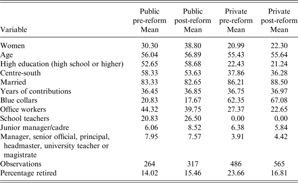
Table 4 reports descriptive statistics for the sample of individuals, separately for public and private workers (respectively, the control and the treatment group) and pre- and post-reform periods (2002–04 and 2006–08 respectively). The share of women is higher in the public sector than in the private sector. The distribution of workers among educational levels seems quite different, with a higher share of individuals with at least high school diploma in the public sector than in the private one. Despite the small sample size, there seems to be a larger presence of public workers and pensioners in the Centre-South of Italy and of private workers and pensioners in the North of Italy. The years of contributions are evenly distributed among sectors, while retirement age is slightly higher for public workers. As regards working categories, most private workers are blue collars (more than 60%), a smaller fraction is composed by office workers (around 25%) and the remaining consists of junior and senior manager or similar positions. As for public workers, the biggest share is composed of office workers (more than 40%), followed by school teachers, blue collars and managers. Finally, at the bottom of the table retirement percentages of public and private workers, before and after the reform, are presented. These show that while the average percentage of retired among public workers qualifying for seniority pension increases of something more than 1 pps (percentage points) in the post-reform period, the same percentage decreases of almost 7 pps for private workers.
Descriptive statistics

Notes: The table reports descriptive statistics by employment sector and pre/post treatment period for the sample used in the estimations. The sample is drawn from the 2002 to 2008 SHIW for a total of 1,632 observations.
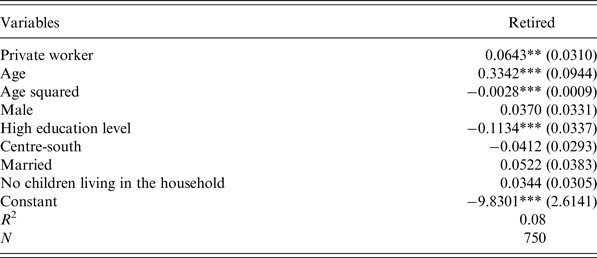
To better analyze the characteristics related to retirement, Table 5 shows the results of a linear model regression for the probability of seniority retirement on the pre-reform sample of individuals. The probability of seniority retirement is 6 pps higher for private than for public workers and, as expected, it is positively and decreasingly correlated with age. It is also negatively correlated with having at least high school diploma, while it is not correlated with sex, geographical area, with being married or with having no children living in the household.
Linear probability model for retirement, pre-reform period

Notes: *p < 0.1; **p < 0.05; ***p < 0.01. Robust standard errors in parentheses.
4 Empirical analysis
4.1 Estimation strategies
Under certain assumptions, it will be possible to compare the behaviour of Italian workers regarding seniority pension before and after the reform, so to study the efficacy of the reform in delaying the retirement decision of private workers, as one would expect given the sizeable economic incentive involved. As individuals who were affected by the reform (private workers) and the individual who was not affected (public workers) may be clearly identified, one can rely on a DID technique. A similar strategy has been used by Bottazzi et al. (Reference Bottazzi, Jappelli and Padula2006), in order to identify the effect of a series of Italian pension reforms on expected retirement age and replacement rate of workers, using old private employees – who were unaffected by the reforms – as a control group.
The classical linear DID is based on an additive structure for potential outcomes in the no-treatment state: in this case, this means assuming that in the absence of the super-bonus, retirement decisions are determined by the sum of a time-invariant effect specific to each category of workers (public/private) and a time effect capturing the common trend. The common trend assumption may be expressed as:
 $$E[Y_{i2}^0 - Y_{i1}^0 \vert X,T] = E[Y_{i2}^0 - Y_{i1}^0 \vert X]$$
where  $Y_{it}^0 $ is the outcome in the no-treatment case, i is the individual, t is time (t = 2 in the post-treatment period, t = 1 in the pre-treatment period), X is a set of covariates and T a treatment dummy.
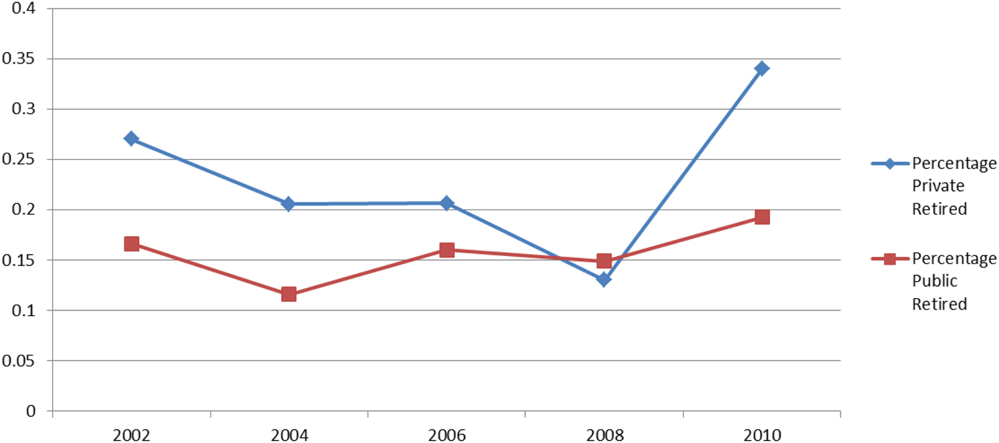
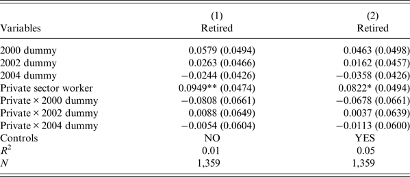
The common trend is not directly testable, but some insight can be gained by looking at seniority retirement percentages through time for public and private workers. These are shown in Figure 5, which shows seniority pension percentages for private and public workers between 2002 and 2010. As explained above, 2002 and 2004 are pre-reform years while 2006 and 2008 are reform years. Although this graph cannot be interpreted as evidence that the common trend assumption is valid, it seems to support it. It is interesting to notice the large jump in the percentage of retired private sector individuals in (post-reform) year 2010, while the percentage of retired public workers remains on similar levels. This seems to further support the presence of an effect of the reform in treatment years, as the distance between the percentage of retired private and public sector workers goes back to pre-treatment levels. As a further check, a LPM of retirement including treated-year interactions is run on pre-reform years (see Table A3 in the Appendix), including years from 1998 to 2004. This leads to the conclusion that there were no significant changes in trend between private and public workers retirement behaviours in pre-reform years.
Percentage retiring among workers qualifying for seniority pension. Notes: The dots in the figure represent the percentage of individuals who retire in that specific year among those who qualify for retirement, by employment sector. The sample is drawn from the 2002 to 2010 SHIW.

Another potential threat to identification in a DID setting is endogenous compositional changes, that could, for example, arise if public workers moved to the private sector because of the reform. Even if it is not possible to test the absence of such compositional changes, it can be argued that they are at least unlikely. First of all, changing sector is not convenient because public sector pensions are in general more generous than private ones and because the public sector has a higher level of job security. Besides, changing job is more costly for older workers and, in fact, uncommon. Overall, being only a temporary measure, it is not likely that the super-bonus had induced public workers to move to the private sector.
Finally, the possibility that the super-bonus was anticipated can be safely ruled out. As explained above, the super-bonus had unique and unprecedented features, especially with respect to the three major reforms of the 1990s.Footnote 17 Besides, the law regulating the bonus was discussed and approved at the end of August 2004Footnote 18 and implemented only slightly more than a month later.
A general model of retirement decision of individual i at time t may be written as:
 $$Y_{it}^{^\ast} = {\beta} ^{\prime}X_{it} + {\tau } ^{\prime}d_t + \varepsilon _{it}$$
where  $Y_{it}^* $ can be interpreted as a latent variable measuring the utility from retiring once seniority pension requirements have been reached. This utility depends on a set of individual characteristics X like age, years of contributions, working sector, earnings, career history and on a vector of time dummies d t to capture trends over time.
Following Wooldridge (Reference Wooldridge2009),Footnote 19 in order to estimate the effect of the reform on the treated when using a sample of pooled independent cross-sections, both a treatment and a post-reform variable must be defined. The former will be a dummy variable T i equal to one for treated individuals, that is private workers and equal to zero for public workers. The latter will be a dummy variable P t equal to one for post-treatment observations, that is those observed in years 2006 and 2008, and equal to zero for the year 2002 and 2004 observations. If  $Y_{it}^* $ were known, one could estimate the effect of the reform by estimating the coefficient α of the interaction between treatment and post-reform dummies, known as DID estimator:
 $$Y_{it}^{^\ast} = {\beta} ^{\prime}X_{it} + {\tau} ^{\prime}d_t + \varphi T_i + \alpha T_iP_t + \varepsilon _{it}$$
while  $Y_{it}^* $ is not observed, a dichotomous variable taking up value one if the eligible individual decides to retire in year t (when
 $Y_{it}^* \ge 0$) or value zero if the individual postponed retirement (when
 $Y_{it}^* \le 0$) may be observed. Even if this naturally leads to a non-linear model, the strategy will be first of all to estimate an ordinary least squares, including the interaction between treatment and post-reform dummies, on the pooled cross-sectional data:
 $$Y_{it} = {\beta} ^{\prime}X_{it} + {\gamma} ^{\prime}P_t + \varphi T_i + \alpha T_iP_t + \varepsilon _{it}$$
In fact, the LPM has often proved to be a very good approximation of probit and logit models and it usually works well for values of the independent variables that are near the averages in the sample (see Wooldridge, Reference Wooldridge2009). The reason why it may be sometimes problematic is that one may get predictions outside the unit interval, as a linear relationship is assumed to hold between the probability and the independent variables. For this reason, as a further robustness check, a DID analysis based on the probit model is provided.
Using probit (or logit) models in place of a LPM, however, it is not a straightforward solution in a DID framework. The issue is that the marginal effects calculated on interaction terms in non-linear models do not allow the DID interpretation that characterizes the coefficient of interaction terms in linear models. Besides, the common trend assumption may not hold for the expectations of Y it (the retirement probabilities) since these may move at different rates depending on baseline probabilities (Blundell et al., Reference Blundell, Dias, Meghir and Reenen2004; Disney et al., Reference Disney, Emmerson and Wakefield2010).Footnote 20 However, this problem can be avoided by assuming that the common trend assumption holds for a transformation of the expectations (retirement probabilities), rather than for the expectations themselves (see Appendix A.3 for a technical discussion of the DID-Probit method and its implementation).
4.2 Results
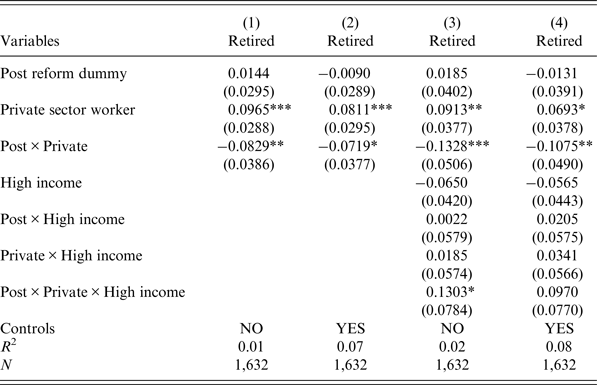
Table 6 reports the results for the DID LPM specification. In column (1) the most basic result is shown. This is obtained by regressing the dichotomous variable for retirement on a set of dummy variables, as explained above. The results indicate that, if assumptions are correct, the super-bonus reform determined a 8 pps reduction in the proportion of private workers who decided to retire among those qualifying for retirement. In column (2), a specification which includes controls for age, age squared, sex, education, area and marital status is presented. A significant reduction in retirement probability of 7 pps is obtained, only slightly smaller than when no controls are included. Table A5 in the Appendix show robustness of the results to the use of a reduced sample, which excludes treated individuals who have reached the contributions requirement, but who have not yet reached seniority pension age (see Section 3).
DID linear probability model

Notes: *p < 0.1; **p < 0.05; ***p < 0.01. Robust standard errors in parentheses. The included pre-treatment years are 2002 and 2004; 2006 and 2008 are treatment years. Regressions include controls for age, age squared, gender, education, geographic area, marital status.
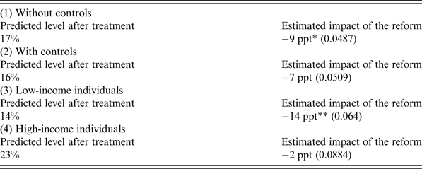
Table 7 reports DID Probit results. Results from row (1) and (2) are in line with LPM results and indicate an even bigger estimated impact of the super-bonus (−9 pps) when no controls are included, and the same reduction when controls are included, even if bootstrapping, in this case, delivers an insignificant result. Overall, these results indicate that the retirement probability of private workers decreased of around 30%, depending on the specification, due to the super-bonus reform.
DID probit

Notes: *p < 0.1; **p < 0.05; ***p < 0.01. Statistical significance estimated using bootstrapping with 500 repetitions. Regressions include controls for age, age squared, gender, education, geographic area, marital status.
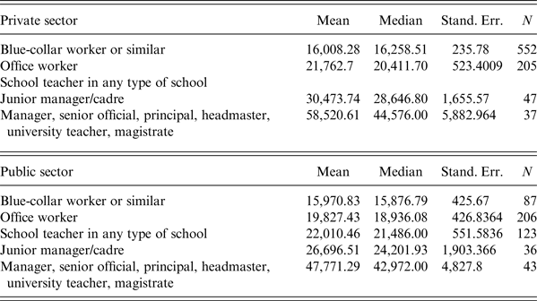
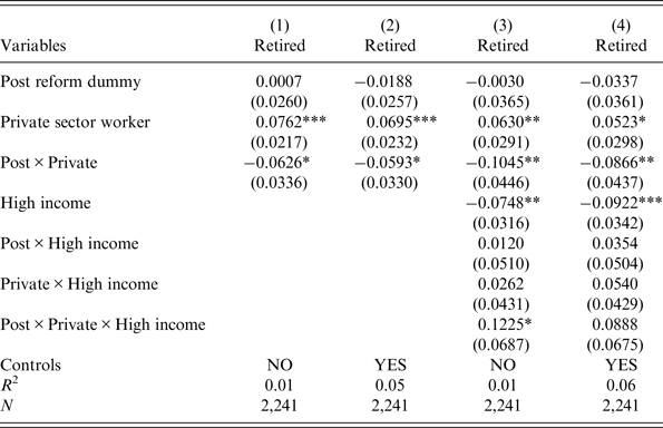
In light of the finding that the bonus is increasing with income (see Section 2), it might be interesting to look at the heterogeneity of results in terms of income. Given the cross-sectional nature of SHIW data, it is not possible to know the pre-retirement labour income of individuals who are already retired at the time of interview. However, SHIW reports the individuals’ current (for workers) and pre-retirement (for pensioners) occupation, which will be used as a proxy of income. Using the information on individuals who are not yet retired, Table A2 in the Appendix shows in fact that individuals’ occupations can be ranked in terms of both mean and median income. In the following, low-income individuals will be defined as blue-collar workers in the private sector and blue-collar and office workers in the public sector. This definition allows to maximize the size of the high- and low-income groups in both sectors, which is important for the precision of estimates as the sample size is small. Most importantly, with this definition the proportion of low- and high-income individuals in the control and treated group is the same,Footnote 21 so that the definition of low- and high-income is consistent across sectors.Footnote 22
Results are shown in column (3) and (4) of Table 6, where a full set of interaction dummies for time, sector and economic condition are included. When no controls are included, a 13 pps reduction in retirement probabilities is estimated for low-income workers, versus a significant-zero reduction for high-income workers. When controls are included, a slightly smaller reduction of 11 pps is observed for low-income workers. DID Probit estimates in Table 7, row (3) and (4), confirm these results.
Overall, these estimations show that the effect of the reform was driven by low-income workers, while the reform was ineffective for high-income workers. This is surprising given that, as shown in details in the next section, the bonus clearly increases with income.
Even if including a shorter pre-treatment period may be preferred in order to more credibly justify the common-trend assumption, Table A4 in the Appendix shows a specification of the DID LPM which includes also 1998 and 2000 as pre-treatment years. Results are between 1 and 2 pps lower in absolute terms than in the main analysis, and still statistically significant.
5 Discussion
In the previous section it was shown that the super-bonus had a sizeable effect on workers’ retirement decisions and that this effect was driven by low-income workers. The latter finding has been found recently for other countries too. Euwals and Trevisan (Reference Euwals and Trevisan2014) show that low wage earners are more sensitive to financial incentives than high wage earners using changes in early retirement conditions of workers in the Netherlands. Mastrobuoni (Reference Mastrobuoni2009) and Hanel and Riphahn (Reference Hanel and Riphahn2012) find stronger responses to retirement incentives for low educated men in the USA and low educated females in Switzerland, respectively: individuals with low education may be expected to also have lower human capital and thus lower wages. Even if it is not possible to give a univocal explanation of these results, a few possibilities may be investigated here.
In general, a reason why higher income workers eligible for seniority retirement might have responded mildly to the reform is that their participation rate was high before the reform (38%) as compared with that of low-income workers (21%). As regards the reasons why low-income workers responded to a small or even negative bonus, liquidity constraints and financial illiteracy are two likely candidates. The intuition for the former is that liquidity constrained individuals may see in the (negative) incentive an opportunity for borrowing against future pension. The intuition for the latter is that financially illiterate individuals may not understand what is the actual incentive offered by the super-bonus, as this involves also detailed knowledge of social security rules.
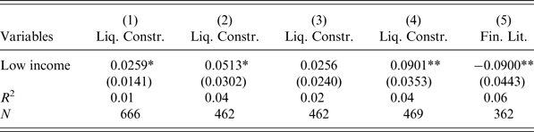
Liquidity constraints can be measured using different definitions, as in Deidda (Reference Deidda2014). Following this work, a first definition can be used which exploits a survey measure of liquidity constraints included in the SHIW. Specifically, individuals are asked if anyone in the household contacted a bank or financial company to obtain a loan or mortgage, and in case of affirmative answer, they are asked if the request was granted in full, granted in part or refused. Individuals are also asked if any member of the household considered applying for a mortgage or a loan but later changed his/her mind thinking the request would be refused. This last question allows to identify discouraged households. Under the first definition, an individual is liquidity constrained if a loan was totally or partially rejected, or if belonging to a discouraged household. Under the second definition, individuals are constrained if their wealth is lower than 2 months income. Under the third definition, individuals are constrained if the ratio of financial liabilities and (the sum of real and financial) assets is higher than 0.5. Under the fourth and final definition, individuals are constrained if they may be defined constrained using at least one of the previous three definitions and non-constrained if they do not result constrained under any of the previous definitions. Results (obtained using a sample comprising only private workers and using years up to 2004, as the super-bonus reform could affect liquidity constraints) are presented in column (1) to (4) of Table 8. Three over four definitions of liquidity constrained individuals deliver a positive and significant relationship between income and liquidity constraints. In particular, low-income individuals have up to 9 pps higher probability of being liquidity constrained.
Income, liquidity constraints and financial literacy

Notes: *p < 0.1; **p < 0.05; ***p < 0.01. Robust standard errors in parentheses. The outcome in column (1) to (4) is a binary variable indicating liquidity constrained individuals. The outcome in column (5) is a binary variable indicating financially literate individuals. Regressions include controls for age, age squared, gender, education, geographic area, marital status. The sample includes private workers in column (1) to (4); private workers and pensioners in column (5). Years 1998 to 2004.
As regards financial illiteracy, some evidence in the literature points to the fact that this could undermine individuals’ ability to internalize new rules in a correct way when affected by reforms of the social security system. Bottazzi et al. (Reference Bottazzi, Jappelli and Padula2006) show that the revision in expectations of retirement age and replacement rate in Italy after the reforms process in the 1900s is limited, and claim that some workers may lack information to fully understand pension rules. Fornero and Monticone (Reference Fornero and Monticone2011), using information on individuals’ financial literacy elicited in the SHIW, show that most individuals lack knowledge of basic financial concepts and that financial literacy has a positive and significant impact on the probability of pension plan participation. Their results also show that women, less educated individuals and individuals living in the South of Italy have worse performances.
As in Fornero and Monticone (Reference Fornero and Monticone2011), some questions about financial literacy first introduced in the SHIW in 2006 are exploited here. These questions are partly similar to those introduced in the Health and Retirement Study and assess knowledge related to concepts like inflation, interest rates, stock market and risk diversification. As the question on inflation is the only one common to all three survey years from 2006 to 2010, only answers to this question are exploited.Footnote 23 In this case, post-reform years may be used as it can be argued that the super-bonus does not affect financial literacy.Footnote 24 An individual is defined as ‘financially literate’ if she responds correctly to the question. Results are presented in column (5) of Table 8 and show that low-income individuals have 9 pps lower probability of being financially literate.
6 Conclusion
Policymakers are often interested in policies that are able to delay retirement and/or increase labour income at older ages. Only very recently, however, taxes have been started to be thought as a possible instrument to do that. This interest, however, is relegated to the economic literature, as in practice younger and older individuals are treated in a similar manner. Social security contributions are an example of a tax that could be used for this purpose; however, there is limited causal evidence on the effect of income tax incentives on retirement behaviour.
This paper contributes to the literature that uses policy evaluation strategies to identify the causal effect of reforms of the pension or social security system on retirement decisions by evaluating the effectiveness of the Italian so-called ‘super-bonus’ reform. This reform was characterized by unique features: it offered to older workers eligible for seniority pensions the possibility to continue working without paying social security contributions but keeping their accrued pension benefits fixed. For this reason, the reform did not have a clear expected effect on individuals’ retirement behaviour: the incentive offered by the super-bonus was negative for most workers, but the reform offered the chance of a higher income today in exchange for lower pension benefits in the future.
As the reform was directed to private workers only, it is possible to use public workers as a counter-factual group. Thus, a DID approach may be exploited and retirement rates of private and public workers before and after the reform may be compared to assess the effect of the reform. A problem with interaction terms in probit models is that, differently from linear models, cannot be interpreted as DID estimators. Thus, a DID estimation strategy proposed by Blundell et al. (Reference Blundell, Dias, Meghir and Reenen2004), appropriate for dichotomous outcome variables, is also employed.
Results suggest that old workers responded to the incentives offered by the reform, as retirement rates among those eligible decreased by around 7 ppt depending on the specification and method used. If assumptions are correct, this means around 30% of those who would have retired chose not to because of the reform. Despite the fact that the true incentive offered by the reform was negative for most workers and increasing with income, regression results also show that the effect of the reform is basically driven by low-income workers (11–14 ppt reduction, depending on the model used). Some evidence on the relationship between income, liquidity constraints and financial literacy of individuals is presented in order to provide some potential, although not definitive nor exhaustive, interpretations of these results. At a minimum, a role for liquidity constraints and financial illiteracy cannot be excluded when interpreting the estimated individuals’ response to the super-bonus reform.
Finally, it should be mentioned that, despite the sizeable causal effect of the super-bonus reform on retirement behaviour found in this paper, it is not possible to claim anything on the efficiency of the reform from this partial analyzes. In fact, it is possible that the cost to the social security system in terms of lost contributions from the workers who would have continued working even in the absence of reform exceeds the gain from those who delay retirement because of the reform. The fiscal cost of the super-bonus, however, may have been offset also by other factors, like taxes paid on labour income and taxes generated by the additional spending of those who postponed retirement.
Conflict of interest
The authors declare that they have no conflict of interest.
A.1 Seniority pension eligibility requirements
Seniority pension eligibility requirements

A.2 Individual labour income by occupation
Income statistics by sector and occupation

A.3 The DID-probit model
The DID-Probit model proposed by Blundell et al. (Reference Blundell, Dias, Meghir and Reenen2004) assumes that the common trend assumption holds for the inverse of the probability function (which is assumed here to be the Normal function Φ( · )) or, in other words, for the index rather than for the probability. Thus, in the absence of treatment, the following equivalence holds:
 $$\matrix{ {\Phi ^{ - 1}[E(Y_{it} \vert X_{it};T_i = 1,P_t = 1)] - \Phi ^{ - 1}[E(Y_{it} \vert X_{it};T_i = 1,P_t = 0)] } \hfill \cr \quad ={\Phi ^{ - 1}[E(Y_{it} \vert X_{it};T_i = 0,P_t = 1)] - \Phi ^{ - 1}[E(Y_{it} \vert X_{it};T_i = 0,P_t = 0)]} \hfill \cr} $$
where Y it is a binary outcome variable, T i is a binary indicator that measures whether an individual was affected by the reform and P t is a binary indicator that measures whether the individual was observed before or after the implementation of the reform. Given the above common trend assumption, the impact of the reform can be evaluated as:
 $$\matrix{ {I(X) = E(Y_{it} \vert X_{it};T_i = 1,P_t = 1) - \Phi \{ \Phi ^{ - 1}[E(Y_{it} \vert X_{it};T_i = 1,P_t = 0)]} \hfill \cr {\quad \quad + \,\Phi ^{ - 1}[E(Y_{it} \vert X_{it};T_i = 0,P_t = 1)] - \Phi ^{ - 1}[E(Y_{it} \vert X_{it};T_i = 0,P_t = 0)]\}} \hfill \cr} $$
Blundell et al. (Reference Blundell, Dias, Meghir and Reenen2004) suggest to implement this estimator of the effect of a policy by estimating four different probit regressions for each of the four groups defined by the interactions of time and treatment. Doing so, it is possible to get an estimate of the behavioural patterns of the four groups, included that triggered by the reform. Then, by predicting the outcome for the treated using the untreated behavioural equations, it is possible to know how the treated would have behaved without the treatment, conditional on their observable characteristics. Finally, plugging these estimates in Equation (5) one can get the estimate of the average impact of the treatment on the treated. This procedure is less restrictive than the usual DID in that it allows for the effect of the treatment to depend on observable characteristics of individuals.Footnote 25
A.4 Tests and robustness checks
Test of the common trend assumption

Robustness to the introduction of more pre-treatment years

Robustness to the use of a different sample

Robustness to the use of a different high/low- income definition