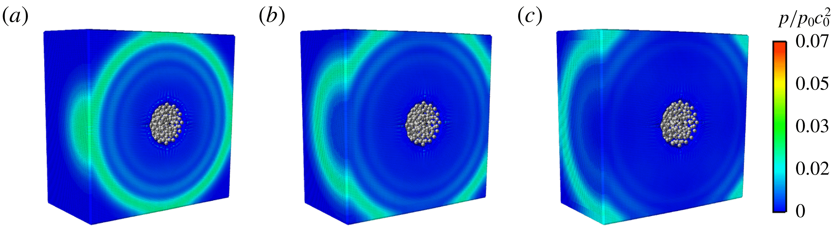
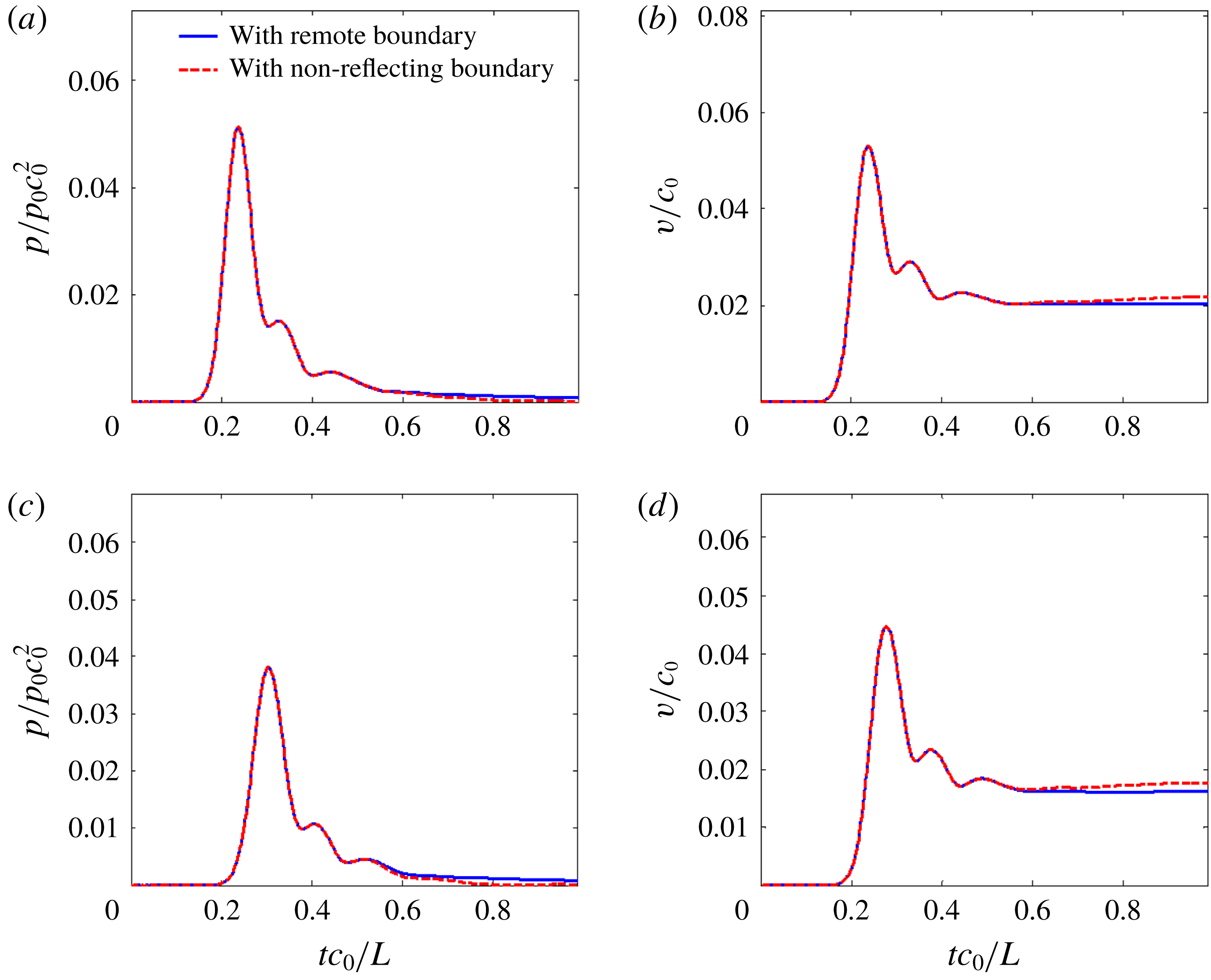
1 Introduction
Computational fluid dynamics (CFD) has been widely used to solve and analyse various hydrodynamic problems. Boundary conditions are one of the key aspects for CFD and special attention should be paid to them. Sometimes, a specific boundary condition should be established to avoid undesirable boundary effects and therefore to model infinite or very large computational domains. That is, a non-reflecting boundary condition (NRBC) is needed. The NRBC is usually divided into two groups, namely the non-local NRBC and the local one. The former is solved based on the information of the whole flow field and can guarantee the solution of a finite domain coincides with that of an infinite domain. However, it is usually limited to linear wave problems with the boundary of specific geometries (see e.g. Givoli Reference Givoli1992, Reference Givoli1999; Alpert, Greengard & Hagstrom Reference Alpert, Greengard and Hagstrom2000; Lubich Reference Lubich2002). For the latter, it is solved only from the information of the neighbouring flow field, which may lead to inaccurate solutions. But it is efficient and easy to implement, and many papers have been published on this topic. Kreiss (Reference Kreiss1970), Engquist & Majda (Reference Engquist and Majda1977) and Thompson (Reference Thompson1990) adopted the characteristic waves method to construct NRBCs for hyperbolic systems, where different waves propagating through boundaries are analysed. This approach is commonly used for Euler equations (see e.g. Poinsot & Lelef Reference Poinsot and Lelef1992; Grinstein Reference Grinstein1994; Baum, Poinsot & Venin Reference Baum, Poinsot and Venin1995; Okong’O & Bellan Reference Okong’O and Bellan2002). Another widely used local NRBC was proposed by Bayliss & Turkel (Reference Bayliss and Turkel1980). The boundary can be placed extremely close to the domain of interest even with strong inhomogeneity, and arbitrary-order accuracy can be obtained by increasing the order of the introduced boundary operator. Besides, the perfect match layer (PML) is also a powerful technique to accomplish NRBCs. It was proposed by Berenger (Reference Berenger1994) and further improvements have been made in the literature (see e.g. Hagstrom Reference Hagstrom1999; Bermúdez et al. Reference Bermúdez, Hervella-Nieto, Prieto and Rodríguez2010). The PML is arranged around the computing domain, and the governing equations in the layer are modified to achieve a perfect match between the PML and the interior domain, so that the outgoing waves inside the layer decay.
As an important branch of CFD, meshless methods are playing an increasingly critical role in simulating fluid dynamics today, among which the smoothed particle hydrodynamics (SPH) method is one of the earliest particle methods. It was first proposed by Gingold & Monaghan (Reference Gingold and Monaghan1977) and Lucy (Reference Lucy1977) in the simulation of astrophysical problems, and Monaghan (Reference Monaghan1994) was the pioneer in applying this method to fluid dynamics. Unlike the traditional grid-based numerical methods, the system in the SPH method is discretized into a set of particles possessing material properties, and the conservative variables of these particles are calculated by using a kernel interpolation. Compared with traditional mesh-based methods, the SPH method presents some remarkable advantages in dealing with problems with free surfaces, large deformations, moving interfaces, etc. Nowadays, the SPH method has been widely used in simulating complex fluid dynamics including free surface flows (Landrini et al. Reference Landrini, Colagrossi, Greco and Tulin2007; Ferrari et al. Reference Ferrari, Fraccarollo, Dumbser, Toro and Armanini2010), surface tension problems (Morris Reference Morris2000) and transport phenomena (Tartakovsky et al. Reference Tartakovsky, Meakin, Scheibe and West2007; Adami, Hu & Adams Reference Adami, Hu and Adams2010).
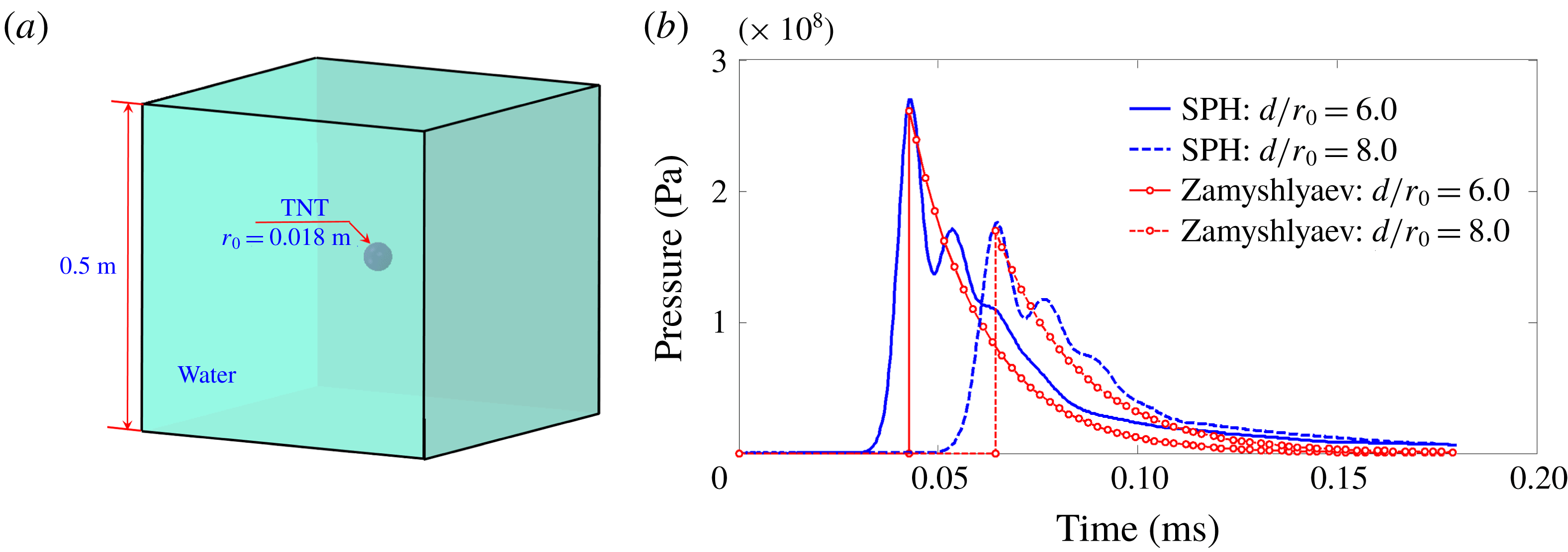
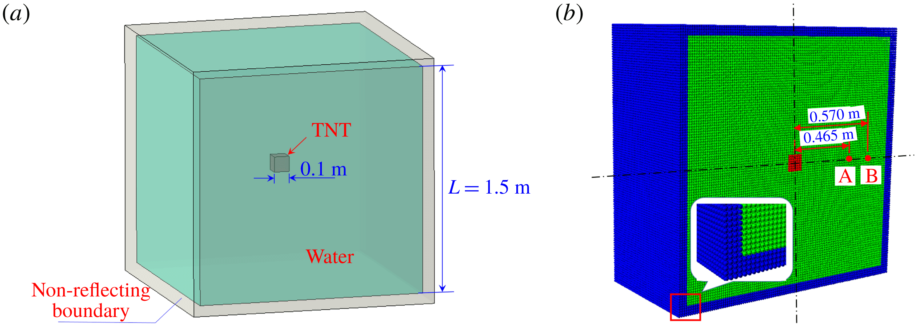
As an important application in fluid dynamics, the SPH method also plays a critical role in the simulation of problems involving an impact, such as underwater explosions and water entries. In these problems, if the computing domain is limited to a small region of interest with inappropriate boundary conditions imposed, the pressure waves reflected from the boundary often have significant effects on the predictions of the pressure and velocity fields. To avoid this problem, an accurate enforcement of the NRBC is particularly important. However, there is still a lack of an accurate and universal NRBC in the SPH method at present because the SPH method presents inherent shortcomings in dealing with boundary conditions. One of the NRBCs in the SPH method is the open boundary condition (see e.g. Morris, Fox & Zhu Reference Morris, Fox and Zhu1997; Lastiwka, Basa & Quinlan Reference Lastiwka, Basa and Quinlan2010; Alvarado-Rodríguez et al. Reference Alvarado-Rodríguez, Klapp, Sigalotti, Domínguez and Sánchez2017; Tafuni et al. Reference Tafuni, Domínguez, Vacondio and Crespo2018), where the spatially fixed inflow and outflow zones are respectively attached to the upstream and downstream of the computational domain. When a particle inside the inflow region enters the fluid domain, a new particle will be created in the inflow region accordingly, while once a particle flows out the outflow region, it will be deleted from the simulation. These boundaries have been used in a wide range of flows (see e.g. Marrone et al. Reference Marrone, Colagrossi, Antuono, Colicchio and Graziani2013; Hou et al. Reference Hou, Kruisbrink, Pearce, Tijsseling and Yue2014; Hirschler et al. Reference Hirschler, Kunz, Huber, Hahn and Nieken2016; Tafuni et al. Reference Tafuni, Domínguez, Vacondio, Sahin and Crespo2016, Reference Tafuni, Domínguez, Vacondio and Crespo2017). Apart from the open boundary condition, another NRBC that should be mentioned in the SPH method is the sponge layer boundary condition. Indeed, there are two types of sponge layer. One is the damping zone introduced by Lind et al. (Reference Lind, Xu, Stansby and Rogers2012) and Altomare et al. (Reference Altomare, Domínguez, Crespo, González-Cao, Suzuki, Gómez-Gesteira and Troch2017) which works by gradually reducing the velocity of the particles in it. The damping zone has been widely used to avoid the reflection of the water waves occurring on the free surface of water. Another type of sponge layer is proposed by Gong, Liu & Wang (Reference Gong, Liu and Wang2009), in which the density variation of the particle belonging to the layer is damped with a factor related to its distance from the boundary. This treatment is convenient for numerical implementation, and has been applied to reduce the reflections of pressure waves (see e.g. Sun, Ming & Zhang Reference Sun, Ming and Zhang2015). However, its shortcomings are also apparent. For instance, the reflected pressure is not reduced efficiently, and the movement of the fluid particles near the sponge layer is confined. Besides, this sponge layer may bring about considerable computational cost, especially for three-dimensional problems.
In this paper, we develop an accurate and efficient NRBC to obtain the propagation and evolution of both the pressure and velocity information at the fluid boundary. It is performed by several layers of boundary particles whose pressures and velocities are updated using the timeline interpolations based on the method of characteristics. This interpolation scheme is derived from the propagation of characteristic waves between particles. The present NRBC is different from some previous NRBCs in SPH (e.g. the outflow boundary condition proposed by Tafuni et al. (Reference Tafuni, Domínguez, Vacondio and Crespo2018) and the sponge layer introduced by Gong et al. (Reference Gong, Liu and Wang2009)). In those boundary conditions, the updating of the physical quantities of boundary particles is usually based on the particle approximation, which is conducted by summing the contributions of all the neighbouring particles within a given particle’s own support domain. Obviously, the particle approximation is essentially a kind of spatial interpolation. In the proposed NRBC, a timeline interpolation rather than a spatial interpolation is adopted to update the physical quantities of the boundary particles. The timeline interpolation scheme is capable of describing the evolution of the pressure and velocity information in fluids more precisely, thus the NRBC can be enforced more accurately for both pressure and velocity fields. This is the first novelty of the proposed NRBC. Another novelty lies in its simplicity and efficiency. Because four layers of boundary particles need to be arranged outside the fluid domain (the number of boundary particles is significantly reduced with respect to the sponge layer proposed by Gong et al. (Reference Gong, Liu and Wang2009)) and the interpolation algorithm adopted is very simple, this NRBC is efficient and easy to implement. The third novelty of the proposed NRBC is its wide applicability. Since the interpolation applied in this NRBC is independent of particle velocities and local sound speed, the proposed NRBC is appropriate for hydrodynamics ranging from low to high speed, viscous or non-viscous flows.
This paper is organized as follows: in § 2 the introduction of the SPH method is provided. Then, in § 3 the method of characteristics is firstly introduced, and based on it, a novel NRBC is proposed within the SPH framework. The influence of numerical parameters on the non-reflection effects is also discussed. Section 4 consists of several examples of the proposed NRBC implementations to further validate the accuracy and stability of this NRBC. Finally, some conclusions will wrap up the paper.
2 The SPH method
2.1 Governing equations for fluid dynamics
In numerical simulations, the fluid dynamics is usually solved by governing equations, including the continuity equation, the momentum equation and the energy equation. Here we focus on an inviscid fluid, and in this case, the governing equations (i.e. Euler equations) in Lagrangian form are
 $$\begin{eqnarray}\left.\begin{array}{@{}c@{}}\displaystyle \frac{\text{D}\unicode[STIX]{x1D70C}}{\text{D}t}=-\unicode[STIX]{x1D70C}\unicode[STIX]{x1D735}\boldsymbol{\cdot }\boldsymbol{u},\\ \displaystyle \frac{\text{D}\boldsymbol{u}}{\text{D}t}=-\frac{\unicode[STIX]{x1D735}p}{\unicode[STIX]{x1D70C}}+\boldsymbol{g},\\ \displaystyle \frac{\text{D}e}{\text{D}t}=-\frac{p}{\unicode[STIX]{x1D70C}}\unicode[STIX]{x1D735}\boldsymbol{\cdot }\boldsymbol{u},\end{array}\right\}\end{eqnarray}$$
where
 $\unicode[STIX]{x1D70C},\boldsymbol{u},e,p$
are respectively the fluid density, velocity, specific internal energy and pressure, and
 $\boldsymbol{g}$
denotes the gravitational acceleration.
To solve the differential equations presented in (2.1), there are mainly two steps in the SPH method, namely kernel approximation of field functions and particle approximation. In the first step, a generic field function
 $f(\boldsymbol{x})$
at a certain position
 $\boldsymbol{x}$
is represented by the integration of the multiplication of
 $f(\boldsymbol{x}^{\prime })$
and a weighting function
 $W$
over the support domain
 $\unicode[STIX]{x1D6FA}$
as follows (Liu & Liu Reference Liu and Liu2003):
 $$\begin{eqnarray}f(\boldsymbol{x})\approx \langle \,f(\boldsymbol{x})\rangle =\int _{\unicode[STIX]{x1D6FA}}f(\boldsymbol{x}^{\prime })W(\boldsymbol{x}-\boldsymbol{x}^{\prime },h)\,\text{d}\boldsymbol{x}^{\prime },\end{eqnarray}$$
in which
 $\langle \,f(\boldsymbol{x})\rangle$
denotes the kernel approximation of
 $f(\boldsymbol{x})$
and
 $\boldsymbol{x}^{\prime }$
is the position in the support domain of
 $\boldsymbol{x}$
. The weighting function
 $W(\boldsymbol{x}-\boldsymbol{x}^{\prime },h)$
, which is often called the kernel function in the SPH literature, has a compact support domain
 $\unicode[STIX]{x1D6FA}$
whose radius is
 $kh$
, where
 $h$
denotes the smoothing length and
 $k$
is a parameter varying with the chosen kernel function. When
 $kh$
tends to zero, the kernel function converges to a delta Dirac function and
 $\langle \,f(\boldsymbol{x})\rangle$
is exactly equal to
 $f(\boldsymbol{x})$
. The kernel function is usually chosen to be a positive even function satisfying
 $\int W(\boldsymbol{x}-\boldsymbol{x}^{\prime },h)\,\text{d}\boldsymbol{x}^{\prime }=1$
with some other conditions which are detailed in Liu & Liu (Reference Liu and Liu2003).
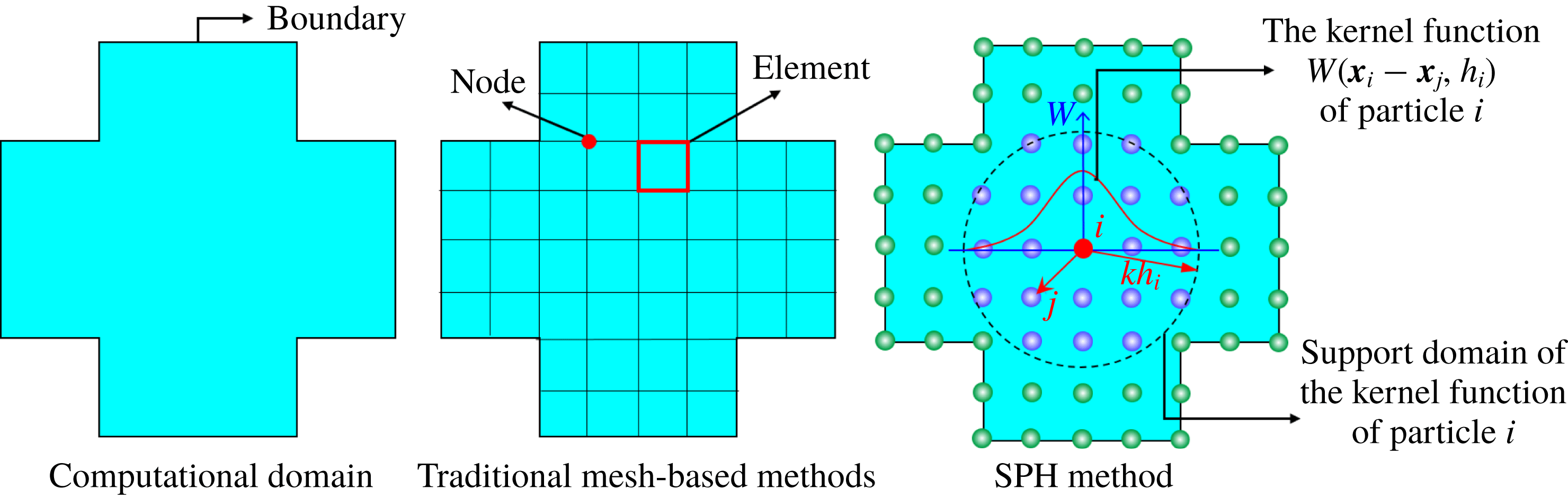
To convert the continuous integration presented in (2.2) to a discretized form. The second step, i.e. the particle approximation, is conducted. Different from the traditional mesh-based methods, in the SPH method, the whole computational domain is discretized into a collection of particles possessing material properties, including pressure, velocity, density, etc., as depicted in figure 1. Therefore, the continuous integration in (2.2) can be replaced by the summation of the particles in the support domain. Thus one can get (Liu & Liu Reference Liu and Liu2003)
 $$\begin{eqnarray}\langle \,f(\boldsymbol{x}_{i})\rangle =\mathop{\sum }_{j}f(\boldsymbol{x}_{j})W(\boldsymbol{x}_{i}-\boldsymbol{x}_{j},h_{i})V_{j},\end{eqnarray}$$
in which
 $i$
represents the particle to be solved and
 $j$
is the particle in the support domain of particle
 $i$
.
 $V_{j}$
is the particle volume solved by
 $m_{j}/\unicode[STIX]{x1D70C}_{j}$
, where
 $m_{j}$
and
 $\unicode[STIX]{x1D70C}_{j}$
are the mass and density of particle
 $j$
, respectively.
Generally, the gradient of the scaler function
 $f(\boldsymbol{x})$
and the divergence of the vector function
 $\boldsymbol{f}(\boldsymbol{x})$
are field functions. Their particle approximations can be obtain by substituting the function
 $f(\boldsymbol{x}_{i})$
in (2.3) with
 $\unicode[STIX]{x1D735}_{i}\,f(\boldsymbol{x}_{i})$
and
 $\unicode[STIX]{x1D735}_{i}\boldsymbol{\cdot }\boldsymbol{f}(\boldsymbol{x}_{i})$
, respectively. The particle approximations of
 $\unicode[STIX]{x1D735}_{i}\,f(\boldsymbol{x}_{i})$
and
 $\unicode[STIX]{x1D735}_{i}\boldsymbol{\cdot }\boldsymbol{f}(\boldsymbol{x}_{i})$
are respectively
 $$\begin{eqnarray}\langle \unicode[STIX]{x1D735}_{i}\,f(\boldsymbol{x}_{i})\rangle =\mathop{\sum }_{j}f(\boldsymbol{x}_{j})\unicode[STIX]{x1D735}_{i}W(\boldsymbol{x}_{i}-\boldsymbol{x}_{j},h_{i})V_{j}\end{eqnarray}$$
and
 $$\begin{eqnarray}\langle \unicode[STIX]{x1D735}_{i}\boldsymbol{\cdot }\boldsymbol{f}(\boldsymbol{x}_{i})\rangle =\mathop{\sum }_{j}\boldsymbol{f}(\boldsymbol{x}_{j})\boldsymbol{\cdot }\unicode[STIX]{x1D735}_{i}W(\boldsymbol{x}_{i}-\boldsymbol{x}_{j},h_{i})V_{j},\end{eqnarray}$$
where the symbol
 $\unicode[STIX]{x1D735}_{i}$
indicates differentiation with respect to the coordinates of particle
 $i$
.
Comparison of conceptual diagrams between traditional mesh-based methods and the SPH method. Different from the traditional mesh-based methods, in the SPH method, the whole computational domain is discretized into a collection of particles whose physical quantities are obtained by interpolating the quantities of particles in their own support domain with the kernel function
 $W$
. The radius of the circular support domain is
 $kh$
.

Therefore, by using (2.4) and (2.5), together with symmetrization processing, the governing equations given by (2.1) can be discretized into the following forms
 $$\begin{eqnarray}\left.\begin{array}{@{}c@{}}\displaystyle \frac{\text{D}\unicode[STIX]{x1D70C}_{i}}{\text{D}t}=\unicode[STIX]{x1D70C}_{i}\mathop{\sum }_{j}(\boldsymbol{u}_{i}-\boldsymbol{u}_{j})\boldsymbol{\cdot }\unicode[STIX]{x1D735}_{i}W_{ij}V_{j},\\ \displaystyle \frac{\text{D}\boldsymbol{u}_{i}}{\text{D}t}=-\mathop{\sum }_{j}\frac{p_{i}+p_{j}}{\unicode[STIX]{x1D70C}_{i}}\unicode[STIX]{x1D735}_{i}W_{ij}V_{j}+\boldsymbol{g},\\ \displaystyle \frac{\text{D}e_{i}}{\text{D}t}=\frac{1}{2}\mathop{\sum }_{j}\frac{p_{i}+p_{j}}{\unicode[STIX]{x1D70C}_{i}}(\boldsymbol{u}_{i}-\boldsymbol{u}_{j})\boldsymbol{\cdot }\unicode[STIX]{x1D735}_{i}W_{ij}V_{j},\end{array}\right\}\end{eqnarray}$$
where
 $W_{ij}=W(|\boldsymbol{x}_{i}-\boldsymbol{x}_{j}|,h_{i})$
represents the kernel function;
 $h_{i}$
denotes the smoothing length of the
 $i$
th particle and it is set to a constant equal to 1.2 times the initial particle spacing in the present work. In particular, an improved Gaussian kernel (Grenier et al.
Reference Grenier, Antuono, Colagrossi, Le and Alessandrini2009) with a support radius equal to
 $3h$
is used for all the simulations in this paper. To stabilize the numerical scheme, it is a common practice in the SPH method to add an artificial viscosity term to the right-hand side of the momentum and energy equations. Here the artificial viscosity terms
 $\unicode[STIX]{x1D6F1}_{I}$
and
 $\unicode[STIX]{x1D6F1}_{II}$
introduced by Monaghan & Gingold (Reference Monaghan and Gingold1983) are applied, whose forms in the momentum and energy equations are respectively
 $$\begin{eqnarray}\unicode[STIX]{x1D6F1}_{I}=\unicode[STIX]{x1D6FC}h_{i}c_{0}\mathop{\sum }_{j}\unicode[STIX]{x1D70B}_{ij}\unicode[STIX]{x1D735}_{i}W_{ij}V_{j}\end{eqnarray}$$
and
 $$\begin{eqnarray}\unicode[STIX]{x1D6F1}_{II}=\displaystyle \frac{1}{2}\unicode[STIX]{x1D6FC}h_{i}c_{0}\mathop{\sum }_{j}\unicode[STIX]{x1D70B}_{ij}(\boldsymbol{u}_{i}-\boldsymbol{u}_{j})\boldsymbol{\cdot }\unicode[STIX]{x1D735}_{i}W_{ij}V_{j},\end{eqnarray}$$
where the term
 $\unicode[STIX]{x1D70B}_{ij}$
is defined as
 $$\begin{eqnarray}\unicode[STIX]{x1D70B}_{ij}=\left\{\begin{array}{@{}ll@{}}\displaystyle \frac{(\boldsymbol{u}_{i}-\boldsymbol{u}_{j})\boldsymbol{\cdot }(\boldsymbol{x}_{i}-\boldsymbol{x}_{j})}{{|\boldsymbol{x}_{i}-\boldsymbol{x}_{j}|}^{2}}, & (\boldsymbol{u}_{i}-\boldsymbol{u}_{j})\boldsymbol{\cdot }(\boldsymbol{x}_{i}-\boldsymbol{x}_{j})<0\\ 0 & \text{otherwise.}\end{array}\right.\end{eqnarray}$$
In (2.7) and (2.8), the non-dimensional parameter
 $\unicode[STIX]{x1D6FC}$
is an empirical coefficient. As most of the literature on SPH indicates, its value covers 0.01–1.0 for different problems (see e.g. Monaghan Reference Monaghan1988; Antuono et al.
Reference Antuono, Colagrossi, Marrone and Molteni2010; Marrone et al.
Reference Marrone, Antuono, Colagrossi, Colicchio, Touzé and Graziani2011). In the present work, a commonly used value 0.1 (see e.g. Molteni & Colagrossi Reference Molteni and Colagrossi2009; Antuono et al.
Reference Antuono, Colagrossi, Marrone and Molteni2010; Sun et al.
Reference Sun, Ming and Zhang2015) is applied to all of the numerical simulations.
In general, considering the compressibility of a fluid, the fluid dynamics solved by the SPH method can be classified into two categories, namely, incompressible flows (e.g. water entries) and completely compressible flows (e.g. underwater explosions). The corresponding SPH methods for solving these two flows are called the weakly compressible SPH (WCSPH) method and the completely compressible SPH method, respectively. These two methods are described in more detail in the following subsections.
2.2 SPH formulas for incompressible flows
For the water flow problems in § 4 (including the water entry of a wedge and the flow around a moving circular cylinder in a rectangular box), the Mach number is less than 0.1, and therefore the water can be considered incompressible in these cases. However, if the real sound speed of water is adopted, the corresponding required stable time step, which depends on the condition of Courant–Fredrich–Levy (CFL), is often very small. To obtain a larger time step and thus reduce the computational costs, Monaghan (Reference Monaghan1994) proposed the WCSPH model, which has a wide range of applications in engineering (see e.g. Altomare et al. Reference Altomare, Domínguez, Crespo, González-Cao, Suzuki, Gómez-Gesteira and Troch2017; Cheng, Zhang & Ming Reference Cheng, Zhang and Ming2017; Ming et al. Reference Ming, Zhang, Cheng and Sun2018). In the WCSPH model, the real sound speed is replaced by a proper artificial sound speed whose value should satisfy the approximate incompressible condition, i.e.
 $$\begin{eqnarray}Ma=\frac{\Vert \boldsymbol{u}\Vert }{c}\leqslant 0.1,\end{eqnarray}$$
where
 $Ma$
denotes the Mach number and
 $c$
is the artificial sound speed. According to (2.10), the artificial sound speed must be at least one order of magnitude larger than the maximum flow velocity, i.e.
 $$\begin{eqnarray}c\geqslant 10\max (\Vert \boldsymbol{u}\Vert ).\end{eqnarray}$$
The artificial sound speed obtained by (2.11) can ensure a reasonable time step and meanwhile, guarantee flow characteristics.
In the context of the WCSPH method, the influence of the energy variation on flow characteristics can be ignored when the peak pressure within the flow field is below 1 GPa (Marrone Reference Marrone2012). Thus the energy equation presented in (2.6) is not considered.
Since (2.6) is a non-closed equation, it is a conventional treatment in the SPH method to use a state equation to describe the correlation between the pressure and density. In WCSPH, the widely used Tait state equation is adopted for water, which takes the form of
 $$\begin{eqnarray}p=\frac{c_{0}^{2}\unicode[STIX]{x1D70C}_{0}}{7}\left[\left(\frac{\unicode[STIX]{x1D70C}}{\unicode[STIX]{x1D70C}_{0}}\right)^{7}-1\right],\end{eqnarray}$$
where
 $\unicode[STIX]{x1D70C}_{0}$
is the reference density when the pressure of the particle is zero. In this paper, the reference density of water is set equal to
 $1000~\text{kg}~\text{m}^{-3}$
for all the simulations.
As discussed in Antuono et al. (Reference Antuono, Colagrossi, Marrone and Molteni2010), one of the drawbacks of standard WCSPH is that the pressure field is generally affected by spurious high-frequency noise. To tackle this problem, we can add a proper artificial diffusive term into the right-hand side of the continuity equation to reduce the pressure noise. This treatment is the so-called
 $\unicode[STIX]{x1D6FF}$
-SPH method proposed by Antuono et al. (Reference Antuono, Colagrossi, Marrone and Molteni2010). Indeed, the
 $\unicode[STIX]{x1D6FF}$
-SPH method is a typical variation of the WCSPH method. The artificial diffusive term
 $\unicode[STIX]{x1D6EC}$
in the
 $\unicode[STIX]{x1D6FF}$
-SPH method reads as
 $$\begin{eqnarray}\unicode[STIX]{x1D6EC}=\unicode[STIX]{x1D6FF}h_{i}c_{0}\mathop{\sum }_{j}\unicode[STIX]{x1D713}_{ij}\unicode[STIX]{x1D735}_{i}W_{ij}V_{j},\end{eqnarray}$$
where the parameter
 $\unicode[STIX]{x1D6FF}$
tunes the magnitude of the numerical diffusive contribution in the continuity equation, and it is set equal to 0.1 for all the simulations. The work of Antuono et al. (Reference Antuono, Colagrossi, Marrone and Molteni2010) shows that
 $\unicode[STIX]{x1D6FF}$
shall be treated as an unadjustable parameter. Besides, the term
 $\unicode[STIX]{x1D713}_{ij}$
in (2.13) is given by
 $$\begin{eqnarray}\unicode[STIX]{x1D713}_{ij}=2(\unicode[STIX]{x1D70C}_{i}-\unicode[STIX]{x1D70C}_{j})\frac{(\boldsymbol{x}_{i}-\boldsymbol{x}_{j})}{{|\boldsymbol{x}_{i}-\boldsymbol{x}_{j}|}^{2}}-(\langle \unicode[STIX]{x1D735}\unicode[STIX]{x1D70C}\rangle _{i}^{L}+\langle \unicode[STIX]{x1D735}\unicode[STIX]{x1D70C}\rangle _{j}^{L})\end{eqnarray}$$
in which the symbol
 $\langle \unicode[STIX]{x1D735}\unicode[STIX]{x1D70C}\rangle _{i}^{L}$
indicates the renormalized density gradient defined in Randles & Libersky (Reference Randles and Libersky1996).
2.3 SPH formulas for completely compressible flows
For underwater explosions, the Mach number is usually greater than 0.1. Thus the real compressibility of water should be considered and the real sound speed of water is adopted. Besides, because of the consideration of internal energy variation, the energy equation should be applied, and the pressure of water is given through the Mie–Gruneisen equation of state (Steinberg Reference Steinberg1987). When the water is in a compressive state, its pressure is given by
 $$\begin{eqnarray}p=\displaystyle \frac{\unicode[STIX]{x1D70C}_{0}c_{0}^{2}\unicode[STIX]{x1D707}\left[1+\left(1-\displaystyle \frac{\unicode[STIX]{x1D6FE}_{0}}{2}\right)\unicode[STIX]{x1D707}-\displaystyle \frac{a}{2}\unicode[STIX]{x1D707}^{2}\right]}{\left[1-(S_{1}-1)\unicode[STIX]{x1D707}-S_{2}\displaystyle \frac{\unicode[STIX]{x1D707}^{2}}{\unicode[STIX]{x1D707}+1}-S_{3}\displaystyle \frac{\unicode[STIX]{x1D707}^{3}}{(\unicode[STIX]{x1D707}+1)^{2}}\right]^{2}}+(\unicode[STIX]{x1D6FE}_{0}+a\unicode[STIX]{x1D707})e,\end{eqnarray}$$
while in the case of expansion, the pressure of the water is given by
 $$\begin{eqnarray}p=\unicode[STIX]{x1D70C}_{0}c_{0}^{2}\unicode[STIX]{x1D707}+(\unicode[STIX]{x1D6FE}_{0}+a\unicode[STIX]{x1D707})e,\end{eqnarray}$$
where the variable
 $\unicode[STIX]{x1D707}$
is defined as
 $\unicode[STIX]{x1D707}=\unicode[STIX]{x1D70C}/\unicode[STIX]{x1D70C}_{0}-1$
;
 $\unicode[STIX]{x1D707}>0$
means that water is in compressed state while
 $\unicode[STIX]{x1D707}<0$
implies an expanded state.
 $\unicode[STIX]{x1D6FE}_{0}$
is the Gruneisen coefficient and
 $a$
represents the volume correction coefficient.
 $S_{1}$
,
 $S_{2}$
and
 $S_{3}$
are experimental fitting coefficients. Parameters in (2.15) and (2.16) are listed in table 1.
Material parameters and coefficients in the Gruneisen state equation for water.

In underwater explosions the cavitation of water will occur and affect the shock loading. However, the cavitation is not the concern of this paper. Thus a simple cutoff model is adopted to describe the cavitation, i.e. when the water pressure is lower than zero, it is simply set to zero. This treatment can also be seen in Xie, Liu & Khoo (Reference Xie, Liu and Khoo2006) and Ming et al. (Reference Ming, Zhang, Xue and Wang2016).
For explosive products produced by the detonation of trinitrotoluene (TNT) the state equation of Jones–Wilkins–Lee (JWL) (Dobratz Reference Dobratz1981) is employed. The pressure of the explosive products is given by
 $$\begin{eqnarray}p=A\left(1-\frac{\unicode[STIX]{x1D714}\unicode[STIX]{x1D702}}{R_{1}}\right)\text{e}^{-R_{1}/\unicode[STIX]{x1D702}}+B\left(1-\frac{\unicode[STIX]{x1D714}\unicode[STIX]{x1D702}}{R_{2}}\right)\text{e}^{-R_{2}/\unicode[STIX]{x1D702}}+\unicode[STIX]{x1D714}\unicode[STIX]{x1D702}\unicode[STIX]{x1D70C}_{0}e,\end{eqnarray}$$
where
 $\unicode[STIX]{x1D702}$
indicates the ratio of the density of the detonation products to the initial density of the original explosive, i.e.
 $\unicode[STIX]{x1D702}=\unicode[STIX]{x1D70C}/\unicode[STIX]{x1D70C}_{0}$
.
 $A$
,
 $B$
,
 $R_{1}$
,
 $R_{2}$
and
 $\unicode[STIX]{x1D714}$
are fitting coefficients. The values of these parameters are given in table 2.
Material parameters and coefficients in the JWL state equation for explosive products.

In addition, because the large deformation of an explosive gas tends to cause inhomogenous spatial distribution of particles, the smoothing length of particles should be updated as (Benz Reference Benz1990)
 $$\begin{eqnarray}h_{i}^{n+1}=h_{i}^{n}-\frac{1}{d}\frac{h_{i}^{n}}{\unicode[STIX]{x1D70C}_{i}^{n}}\frac{\text{D}\unicode[STIX]{x1D70C}_{i}^{n}}{\text{D}t}\unicode[STIX]{x0394}t,\end{eqnarray}$$
where
 $h_{i}^{n}$
and
 $\unicode[STIX]{x1D70C}_{i}^{n}$
denote respectively the smoothing length and density of the
 $i$
th particle at the
 $n$
th time step;
 $d$
is the number of spatial dimensions and
 $\unicode[STIX]{x0394}t$
represents the size of the time step.
2.4 Boundary implementation and time integration
In this subsection, several boundary conditions used in the present work are introduced, including the outflow boundary condition, the sponge layer boundary condition and the solid boundary condition. Additionally, the time integration scheme applied is also illustrated.
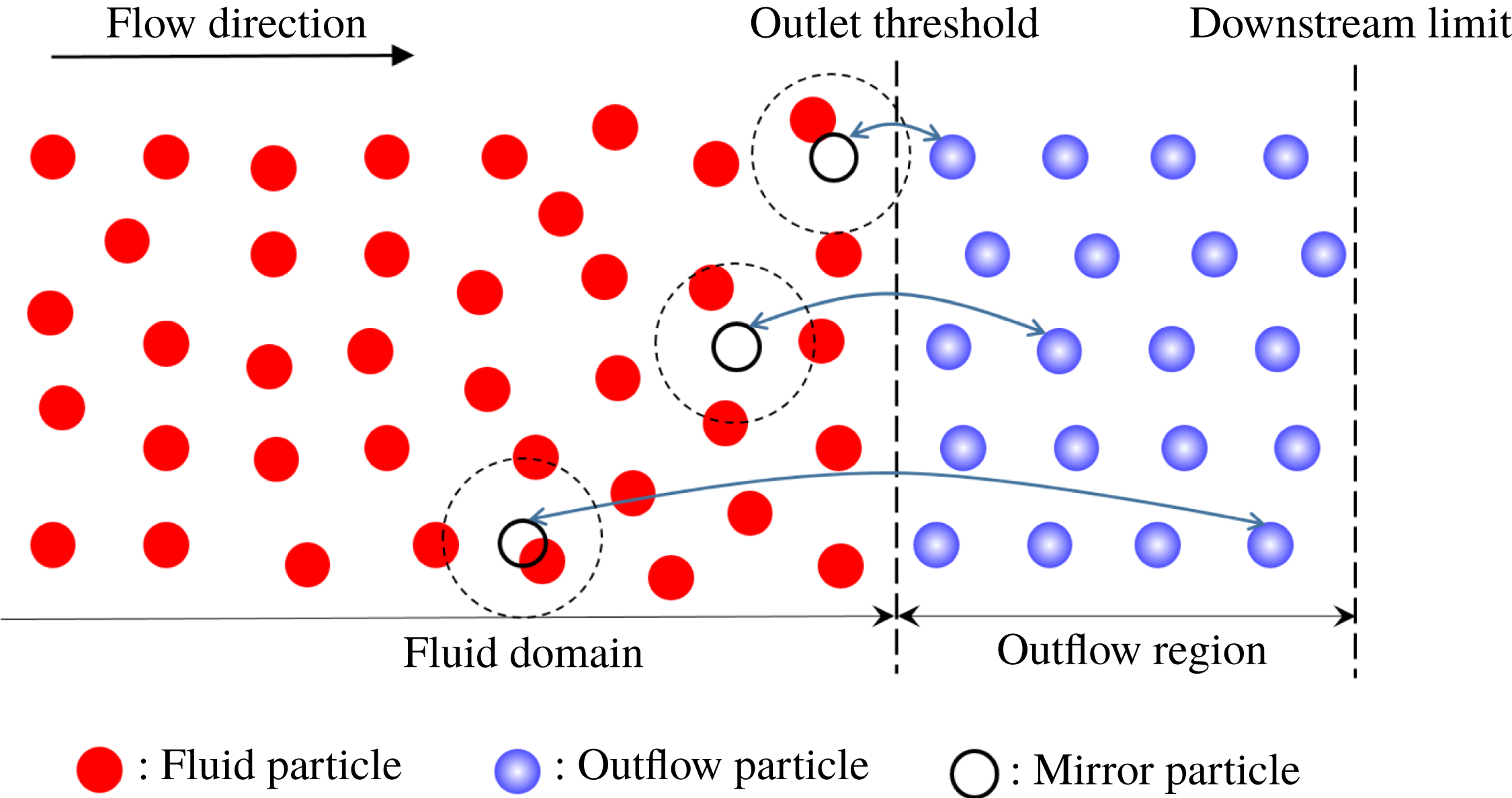
Schematic diagram of the outflow boundary condition proposed by Tafuni et al. (Reference Tafuni, Domínguez, Vacondio and Crespo2018) for two-dimensional models. The fluid particles entering the outflow region are transformed into outflow particles, while the outflow particles passing through the downstream limit of the outflow region are eliminated from the simulation. The pressure and velocity interpolations are firstly carried out at the mirror particles which are the instantaneous mirrors of the outflow particles with respect to the outlet threshold. Then the physical quantities of the mirror particles are projected back to the corresponding outflow particles by using the first-order Taylor series expansion.

2.4.1 Outflow boundary
In the SPH method, an alternative to reduce the undesirable wave reflections is to impose open boundary conditions outside the computational domain. Recently, a versatile open boundary condition is developed by Tafuni et al. (Reference Tafuni, Domínguez, Vacondio and Crespo2018). It can be used for the inflow, outflow and mixed open boundary conditions, and has been successfully implemented in the simulations of two-dimensional (2-D) and 3-D complex flows (see more details in Tafuni et al.
Reference Tafuni, Domínguez, Vacondio, Sahin and Crespo2016, Tafuni et al.
Reference Tafuni, Domínguez, Vacondio and Crespo2017). In this paper, considering the problems to be solved, only the outflow boundary condition is applied, and its schematic is displayed in figure 2. The outflow region, whose width should be comparable to or greater than the support radius of fluid particles, is defined downstream of the fluid domain. The particles in the fluid domain and the outflow region are called fluid particles and outflow particles, respectively. When the fluid particles flow out of the fluid domain and enter the outflow region, they are transformed into outflow particles. Once the outflow particles flow past the downstream limit of the outflow region, they are eliminated from the simulation. To update the physical quantities of the outflow particles, the pressure and velocity interpolations are firstly carried out at the mirror particles which are the instantaneous mirrors of the outflow particles with respect to the outlet threshold. However, a standard SPH interpolation tends to yield poor results due to the kernel truncation near the boundary. Therefore, a correction can be made to restore the consistency of the kernel function (Liu & Liu Reference Liu and Liu2006; Huang et al.
Reference Huang, Zhang, Shi, Si and Huang2018). If we note
 $R_{m}$
and
 $R_{m,\unicode[STIX]{x1D6FD}}$
respectively the approximation of the physical quantities of mirror particles and their first-order spatial derivatives, they can be obtained as
 $$\begin{eqnarray}R_{m}=\left|\begin{array}{@{}cc@{}}\displaystyle \mathop{\sum }_{j}R_{j}W_{mj}V_{j} & \displaystyle \mathop{\sum }_{j}(\boldsymbol{x}_{j}^{\unicode[STIX]{x1D6FD}}-\boldsymbol{x}_{m}^{\unicode[STIX]{x1D6FD}})W_{mj}V_{j}\\ \displaystyle \mathop{\sum }_{j}R_{j}W_{mj,\unicode[STIX]{x1D6FE}}V_{j} & \displaystyle \mathop{\sum }_{j}(\boldsymbol{x}_{j}^{\unicode[STIX]{x1D6FD}}-\boldsymbol{x}_{m}^{\unicode[STIX]{x1D6FD}})W_{mj,\unicode[STIX]{x1D6FE}}V_{j}\end{array}\right|\left/\left|\begin{array}{@{}cc@{}}\displaystyle \mathop{\sum }_{j}W_{mj}V_{j} & \displaystyle \mathop{\sum }_{j}(\boldsymbol{u}_{j}^{\unicode[STIX]{x1D6FD}}-\boldsymbol{u}_{m}^{\unicode[STIX]{x1D6FD}})W_{mj}V_{j}\\ \displaystyle \mathop{\sum }_{j}W_{mj,\unicode[STIX]{x1D6FE}}V_{j} & \displaystyle \mathop{\sum }_{j}(\boldsymbol{x}_{j}^{\unicode[STIX]{x1D6FD}}-\boldsymbol{x}_{m}^{\unicode[STIX]{x1D6FD}})W_{mj,\unicode[STIX]{x1D6FE}}V_{j}\end{array}\right|,\right.\end{eqnarray}$$
 $$\begin{eqnarray}R_{m,\unicode[STIX]{x1D6FD}}=\left.\left|\begin{array}{@{}cc@{}}\displaystyle \mathop{\sum }_{j}W_{mj}V_{j} & \displaystyle \mathop{\sum }_{j}R_{j}W_{mj}V_{j}\\ \displaystyle \mathop{\sum }_{j}W_{mj,\unicode[STIX]{x1D6FE}}V_{j} & \displaystyle \mathop{\sum }_{j}R_{j}W_{mj,\unicode[STIX]{x1D6FE}}V_{j}\end{array}\right|\right/\left|\begin{array}{@{}cc@{}}\displaystyle \mathop{\sum }_{j}W_{mj}V_{j} & \displaystyle \mathop{\sum }_{j}(\boldsymbol{x}_{j}^{\unicode[STIX]{x1D6FD}}-\boldsymbol{x}_{m}^{\unicode[STIX]{x1D6FD}})W_{mj}V_{j}\\ \displaystyle \mathop{\sum }_{j}W_{mj,\unicode[STIX]{x1D6FE}}V_{j} & \displaystyle \mathop{\sum }_{j}(\boldsymbol{x}_{j}^{\unicode[STIX]{x1D6FD}}-\boldsymbol{x}_{m}^{\unicode[STIX]{x1D6FD}})W_{mj,\unicode[STIX]{x1D6FE}}V_{j}\end{array}\right|,\end{eqnarray}$$
where the subscript
 $m$
denotes the mirror particle, and
 $j$
represents the fluid particle inside the support domain of particle
 $m$
.
 $\unicode[STIX]{x1D6FD}$
and
 $\unicode[STIX]{x1D6FE}$
are the dimension indexes repeated from 1 to
 $d$
.
 $W_{mj,\unicode[STIX]{x1D6FE}}=\unicode[STIX]{x2202}W_{mj}/\unicode[STIX]{x2202}\boldsymbol{x}^{\unicode[STIX]{x1D6FE}}$
is the spatial derivative of the kernel function. For this outflow boundary condition, the pressure and velocity of the mirror particles are calculated through (2.19), and then these physical quantities are projected back to the corresponding outflow particles by using the first-order Taylor series expansion as follows
 $$\begin{eqnarray}R_{n}=R_{m}+(\boldsymbol{x}_{n}^{\unicode[STIX]{x1D6FD}}-\boldsymbol{x}_{m}^{\unicode[STIX]{x1D6FD}})R_{m,\unicode[STIX]{x1D6FD}},\end{eqnarray}$$
where the subscript
 $n$
represents the outflow particle corresponding to the mirror particle
 $m$
, and the spatial derivative
 $R_{m,\unicode[STIX]{x1D6FD}}$
is obtained by (2.20).
2.4.2 Sponge layer
Sponge layer is another boundary condition that can reduce the wave reflection caused by the truncation of the physical domain. Here the sponge layer proposed by Gong et al. (Reference Gong, Liu and Wang2009) is introduced, which is enforced by arranging dozens of layers of particles around the fluid domain. Regarding the particles in the sponge layer, the time derivatives of density are multiplied by a correction term as follows
 $$\begin{eqnarray}\left(\frac{\text{D}\unicode[STIX]{x1D70C}_{i}}{\text{D}t}\right)=(1-100^{-0.9^{50\unicode[STIX]{x1D706}}})\left(\frac{\text{D}\unicode[STIX]{x1D70C}_{i}}{\text{D}t}\right),\end{eqnarray}$$
where
 $\unicode[STIX]{x1D706}=(s-d)/s$
, in which
 $d$
denotes the distance from the sponge layer particle to the interface between fluid and the sponge layer, and
 $s$
is the thickness of the sponge layer. In addition, the solid wall boundary condition should be applied outside the sponge layer to offer restriction to the fluid flow.
2.4.3 Dummy boundary
In this work, the dummy boundary condition is adopted as the solid boundary condition. It was proposed by Adami, Hu & Adams (Reference Adami, Hu and Adams2012) and has been extensively used to deal with various fluid and bodies interactions (see e.g. Ulrich, Leonardi & Rung Reference Ulrich, Leonardi and Rung2013; Cao, Ming & Zhang Reference Cao, Ming and Zhang2014; Ming, Sun & Zhang Reference Ming, Sun and Zhang2017). It is discretized into several layers of particles distributed along the boundary, and the relative positions of boundary particles do not change during the simulation. The near-boundary fluid particles interact with neighbouring dummy particles to guarantee full support of the kernel interpolation. The pressure of boundary particles is obtained as follows
 $$\begin{eqnarray}p_{w}=\mathop{\sum }_{f}W_{wf}[\unicode[STIX]{x1D70C}_{f}(\boldsymbol{g}-\boldsymbol{a}_{w})\boldsymbol{\cdot }(\boldsymbol{x}_{w}-\boldsymbol{x}_{f})+p_{f}]/\mathop{\sum }_{f}W_{wf},\end{eqnarray}$$
where the subscript
 $f$
denotes the fluid particle while
 $w$
represents the body wall particle. Through solving the equation of state conversely, the density of the dummy particles can be obtained. For all simulations in this work, the free-slip condition is applied, and the equations for describing the rigid body motions can refer to Sun et al. (Reference Sun, Ming and Zhang2015).
2.4.4 Time integration
With respect to the time integration scheme, the predictor–corrector scheme in Monaghan (Reference Monaghan1989) is implemented. To guarantee the numerical stability, the magnitude of the time step
 $\unicode[STIX]{x0394}t$
is limited by the CFL condition (see Monaghan (Reference Monaghan1989) and Morris et al. (Reference Morris, Fox and Zhu1997) for more details). Considering the particle acceleration, viscous diffusion and combined Courant viscous force, the size of the time step is restricted by the following three conditions
 $$\begin{eqnarray}\displaystyle & \displaystyle \unicode[STIX]{x0394}t\leqslant 0.25\sqrt{\frac{h_{i}}{\displaystyle \max _{i}\Vert \boldsymbol{a}\Vert }}, & \displaystyle\end{eqnarray}$$
 $$\begin{eqnarray}\displaystyle & \displaystyle \unicode[STIX]{x0394}t\leqslant 0.125\frac{{h_{i}}^{2}}{\unicode[STIX]{x1D708}}, & \displaystyle\end{eqnarray}$$
 $$\begin{eqnarray}\displaystyle & \displaystyle \unicode[STIX]{x0394}t\leqslant 0.25\min _{i}\left(\frac{h_{i}}{c_{0}+h_{i}\displaystyle \max _{j}\unicode[STIX]{x1D70B}_{ij}}\right), & \displaystyle\end{eqnarray}$$
where
 $\boldsymbol{a}$
denotes the particle acceleration and
 $\unicode[STIX]{x1D708}$
is the kinematic viscosity coefficient. The minimum of the values obtained by the above three conditions is selected as the final time step.
3 Non-reflecting boundary
As discussed in § 1, the NRBC is of great importance to obtain physically meaningful and correct numerical results in simulating some problems, such as underwater explosions and water entries. In this section, a novel NRBC within the SPH framework is presented. Because this NRBC is derived based on the method of characteristics, the method of characteristics is firstly introduced in the following, then the idea of the NRBC within the SPH framework will be presented.
3.1 Method of characteristics
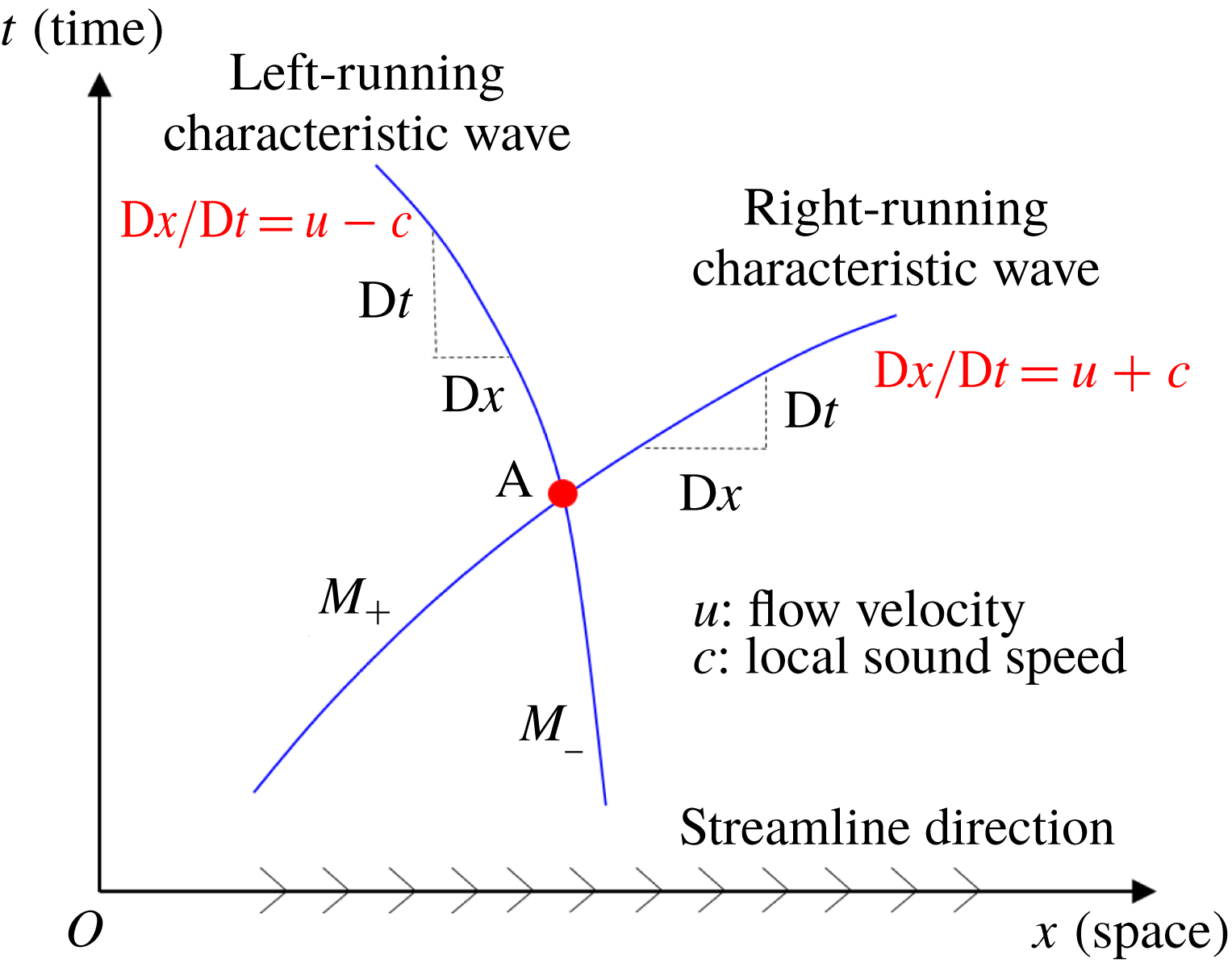
The method of characteristics is one of the conventional methods in CFD for the implementation of boundary conditions because of its simplicity and robustness. For the unsteady, one-dimensional inviscid flow whose governing equations are hyperbolic, it has been proved that there exist two real characteristic lines with slopes
 $\text{D}t/\text{D}x=1/(u+c)$
and
 $\text{D}t/\text{D}x=1/(u-c)$
through a given point A in the
 $x$
–
 $t$
(space–time) plane, as sketched in figure 3, where
 $u$
and
 $c$
denote respectively the flow velocity of fluid and the local speed of sound. These two lines can be interpreted as the trajectories of disturbance or sound waves (often called characteristic waves) carrying the information of specific variables. These variables are so-called characteristic variables whose values are constant along the characteristic lines. The characteristic waves with the propagation velocities
 $\text{D}x/\text{D}t=u-c$
and
 $\text{D}x/\text{D}t=u+c$
are respectively labelled
 $M_{-}$
and
 $M_{+}$
, representing the waves travelling upstream and downstream at the speed of sound (relative to the moving fluid), respectively, and they are called left- and right-running characteristic waves. The method of characteristics solves the flow from the perspective of information propagation, thus providing an effective approach for the implementation of numerical boundary conditions.
The characteristic lines for unsteady, one-dimensional inviscid flow.
 $M_{-}$
and
 $M_{+}$
denote the left- and right-running characteristic waves, respectively, and they can be interpreted as the trajectories of disturbance or sound waves.

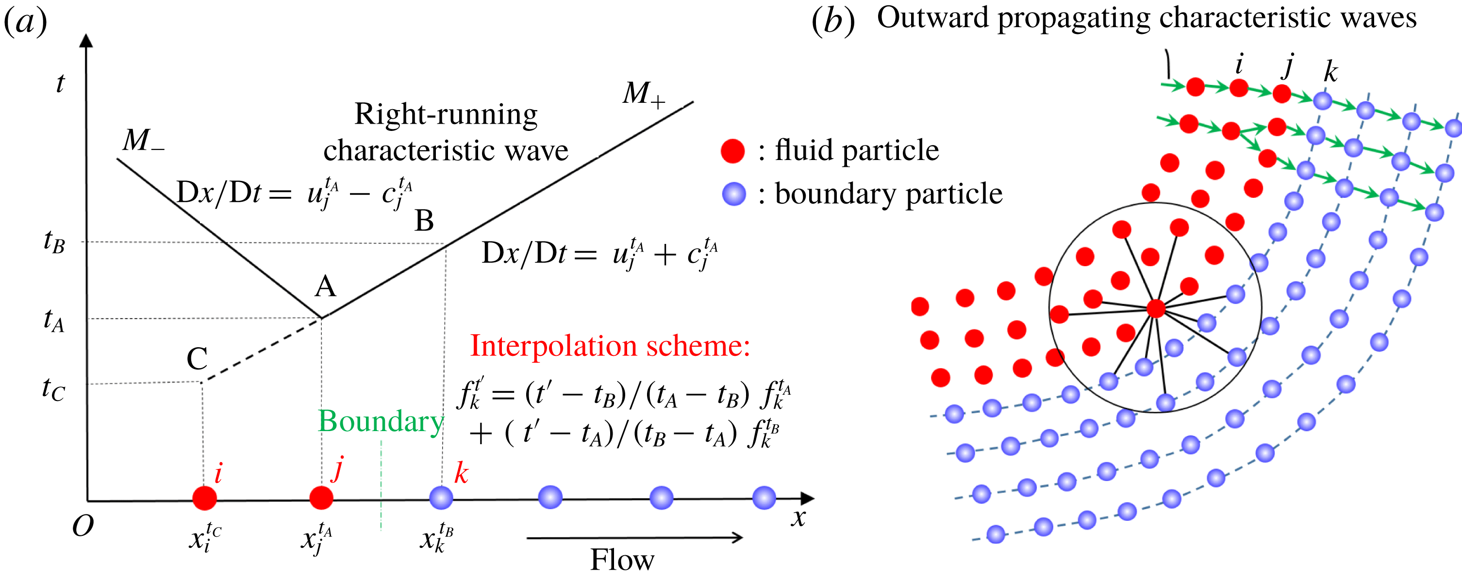
The propagation of the characteristic waves in one-dimensional (a) and two-dimensional (b) models. In the one-dimensional model, the straight line CB can be interpreted as the right-running characteristic wave emitted from the particle
 $i$
at time
 $t_{C}$
, passing through the particle
 $j$
at time
 $t_{A}$
and reaching the particle
 $k$
at time
 $t_{B}$
. Therefore, the physical quantities of the particle
 $k$
at the time
 $t_{B}$
can be predicted by
 $f_{k}^{t_{B}}=f_{j}^{t_{A}}$
, and then their values at a given time
 $t^{\prime }$
(
 $t_{A}\leqslant t^{\prime }\leqslant t_{B}$
) can be evaluated by the Lagrange interpolation in time domain given by (3.2). For the two-dimensional model, the characteristic waves passing through the boundary particles are approximately assumed to be coming from their nearest particles in the inner layer.

3.2 Non-reflecting boundary condition within SPH framework
In this subsection, based on the method of characteristics using timeline interpolations, a novel NRBC in the SPH method is presented. A one-dimensional model is taken to illustrate the non-reflecting boundary algorithm in detail. As figure 4(a) shows, the fluid particles are distributed along the
 $x$
axis at the initial time. The first step of building the NRBC is to place several layers of boundary particles outside the fluid domain, and the thickness of the boundary layer needs to be comparable to or greater than the support radius of the kernel function to guarantee the integrity of the support domain of near-boundary fluid particles. In the present work, four layers of boundary particles are initially positioned. The fluid and boundary particles closest to the boundary are respectively denoted by
 $j$
and
 $k$
, while the fluid particle next to
 $j$
is represented by
 $i$
. The direction of the flow is assumed to be from the fluid particles to the boundary particles.
The second step is to update the physical quantities of the boundary particles by conducting the Lagrange interpolation in the time domain. This interpolation scheme is capable of accurately describing the evolution of pressure and velocity waves. In the following, the updating algorithm of the quantities of particle
 $k$
is presented to illustrate the interpolation scheme in detail. As figure 4(a) shows, the coordinate of particle
 $j$
at time
 $t_{A}$
is noted as
 $x_{j}^{t_{A}}$
. According to the method of characteristics, there exist two characteristic waves
 $M_{-}$
and
 $M_{+}$
through the point A in the
 $x$
–
 $t$
plane. The velocities of
 $M_{-}$
and
 $M_{+}$
are respectively
 $\text{D}x/\text{D}t=u_{j}^{t_{A}}-c_{j}^{t_{A}}$
and
 $\text{D}x/\text{D}t=u_{j}^{t_{A}}+c_{j}^{t_{A}}$
, where
 $u_{j}^{t_{A}}$
and
 $c_{j}^{t_{A}}$
denote the velocity and sound speed of particle
 $j$
at time
 $t_{A}$
, respectively. The moment when the characteristic wave
 $M_{+}$
reaches particle
 $k$
is denoted as
 $t_{B}$
, and the coordinate of particle
 $k$
at
 $t_{B}$
is represented by
 $x_{k}^{t_{B}}$
. The enforcement of NRBCs means that there is no upstream propagating disturbance produced by boundary particles. Besides, it is assumed that the initial perturbation of the boundary particles is zero. Therefore, the fluid particle
 $j$
and the four boundary particles shown in figure 4(a) are only affected by the right-running characteristic waves from upstream. Thus, these characteristic waves can be treated as simple waves, that is, the characteristic lines are straight and all physical quantities are constant along them. Accordingly, the physical quantities for particle
 $k$
at the time
 $t_{B}$
can be obtained as
 $$\begin{eqnarray}f_{k}^{t_{B}}=f_{j}^{t_{A}},\end{eqnarray}$$
where
 $f_{j}^{t_{A}}$
denotes the quantities of particle
 $j$
at time
 $t_{A}$
. Then the physical quantities of particle
 $k$
at a given time
 $t^{\prime }$
(
 $t_{A}\leqslant t^{\prime }\leqslant t_{B}$
) are obtained by a simple Lagrange interpolation in time domain as follows
 $$\begin{eqnarray}f_{k}^{t^{\prime }}=\frac{t^{\prime }-t_{B}}{t_{A}-t_{B}}f_{k}^{t_{A}}+\frac{t^{\prime }-t_{A}}{t_{B}-t_{A}}f_{k}^{t_{B}},\end{eqnarray}$$
where
 $f_{k}^{t_{A}}$
,
 $f_{k}^{t_{B}}$
and
 $f_{k}^{t^{\prime }}$
denote the physical quantities of particle
 $k$
at times
 $t_{A}$
,
 $t_{B}$
and
 $t^{\prime }$
, respectively. In this work, the pressure and velocity of boundary particles are updated by (3.2) while the density is inversely solved through the equation of state. According to the velocities of the boundary particles, their coordinates are updated by
 $\unicode[STIX]{x0394}\boldsymbol{x}_{b}/\unicode[STIX]{x0394}t=\boldsymbol{u}_{b}$
, where
 $\boldsymbol{x}_{b}$
and
 $\boldsymbol{u}_{b}$
are the coordinates and velocities of the boundary particles, respectively. However, one should note that
 $t_{B}$
in (3.2) is unknown. According to the propagation of the characteristic wave
 $M_{+}$
between particles
 $j$
and
 $k$
,
 $t_{B}$
can be calculated by
 $$\begin{eqnarray}t_{B}=t_{A}+\frac{x_{k}^{t_{B}}-x_{j}^{t_{A}}}{c_{j}^{t_{A}}+u_{j}^{t_{A}}},\end{eqnarray}$$
where
 $x_{k}^{t_{B}}$
, representing the coordinate of particle
 $k$
at time
 $t_{B}$
, is unknown. It can be approximately equal to the coordinate at time
 $t_{A}$
(i.e.
 $x_{k}^{t_{B}}=x_{k}^{t_{A}}$
). Then (3.3) becomes
 $$\begin{eqnarray}t_{B}=t_{A}+\frac{x_{k}^{t_{A}}-x_{j}^{t_{A}}}{c_{j}^{t_{A}}+u_{j}^{t_{A}}}.\end{eqnarray}$$
However, it is obvious that (3.4) will lead to an underestimation of
 $t_{B}$
in practice, which tends to result in significant influences on the non-reflection effect, as proved in the following one-dimensional underwater explosion simulation. Therefore, another access to obtain the values of
 $t_{B}$
is proposed in this paper. Since the right-running characteristic waves emitted from
 $i$
,
 $j$
and all boundary particles are all simple waves, it can be determined that the characteristic line
 $M_{+}$
is collinear with the characteristic line emitted from the particle
 $i$
at a certain time. This time is denoted by
 $t_{C}$
, and the coordinate of the particle
 $i$
at time
 $t_{C}$
is represented by
 $x_{i}^{t_{C}}$
. Then the reverse extension of line AB must pass through the point C whose abscissa and ordinate are
 $x_{i}^{t_{C}}$
and
 $t_{C}$
, respectively. Therefore, the straight line CB can be interpreted as the right-running characteristic wave emitted from the particle
 $i$
at time
 $t_{C}$
, passing through the particle
 $j$
at time
 $t_{A}$
and reaching the particle
 $k$
at time
 $t_{B}$
. It is assumed that the time interval for the characteristic waves passing from the particle
 $i$
to
 $j$
is equal to that from
 $j$
to
 $k$
(when the initial particle distribution is uniform), i.e.
 $$\begin{eqnarray}t_{A}-t_{C}=t_{B}-t_{A}.\end{eqnarray}$$
Thus the value of
 $t_{B}$
can be obtained as follows
 $$\begin{eqnarray}t_{B}=2t_{A}-t_{C},\end{eqnarray}$$
where
 $t_{C}$
can be obtained by the relation
 $f_{i}^{t_{C}}=f_{j}^{t_{A}}$
, i.e.
 $t_{C}$
is the moment when the physical quantity of particle
 $i$
is equal to that of particle
 $j$
at time
 $t_{A}$
. In this paper, the pressure is chosen as the quantity to determine the value of
 $t_{C}$
. Thus, the pressure evolutions of the fluid particles
 $i$
and
 $j$
should be recorded at adjacent previous time steps. It is obvious that the method of calculating
 $t_{B}$
given by (3.6) is independent of particle velocities and local sound speed. Therefore, it can be applied to a broad variety of fluid dynamics ranging from low-speed flows to high-speed impacts.
Parameters and particle distributions of the 1-D underwater explosion with the proposed non-reflecting boundary. The fluid particle closest to the boundary is chosen as the measuring point.

When the NRBC is applied to two- and three-dimensional problems, the boundary particles should be initially placed on four paralleled lines or planes outside the fluid domain accordingly. Figure 4(b) depicts a sketch of the non-reflecting boundary in two-dimensional models. For the boundary particle
 $k$
, its closest particle in the inner layer is noted as
 $j$
, and the particle closest to
 $j$
in the inner layer is particle
 $i$
. The pressure and velocity of all boundary particles are updated by (3.2) at every time step, while the quantities of fluid particles are updated by the governing equations. To avoid the kernel truncation error, the fluid particles interact with not only fluid particles nearby but also the boundary particles inside their own support domain.
Subsequently, to demonstrate that (3.6) gives a more accurate estimation of
 $t_{B}$
than (3.4), the simulation of a one-dimensional underwater explosion is performed (the validation of the present SPH procedure for underwater explosions is given in § 4.3). Figure 5 depicts a sketch of the whole model, where the water and TNT particles are regularly distributed along the
 $x$
axis with a particle spacing
 $\unicode[STIX]{x0394}x=0.005~\text{m}$
. The initial density and pressure of TNT are
 $1630~\text{kg}~\text{m}^{-3}$
and zero, respectively. The progressive detonation model for TNT (see e.g. Ming et al.
Reference Ming, Zhang, Xue and Wang2016) is applied and the behaviour of detonation products is described with the JWL state equation. Gravity is not considered in this simulation. There are four particles at both ends of the water domain, and the detonation point is located at the origin
 $O$
. The water particle closest to the boundary is chosen as the measuring point. The solution is depicted up to
 $t=2~\text{ms}$
. Simulations with
 $t_{B}$
evaluated by (3.4) or (3.6) are carried out. Additionally, the free-field underwater explosion with a large water domain is simulated to provide a reference of the exact NRBC. In the reference case, the water domain is set to 3.0 m long while other parameters remain the same, aiming to ensure the shock wave produced by the detonation has not yet reached the boundary at the end of the simulation. This reference case with the large water domain is recognized as the solution with a remote boundary hereinafter.
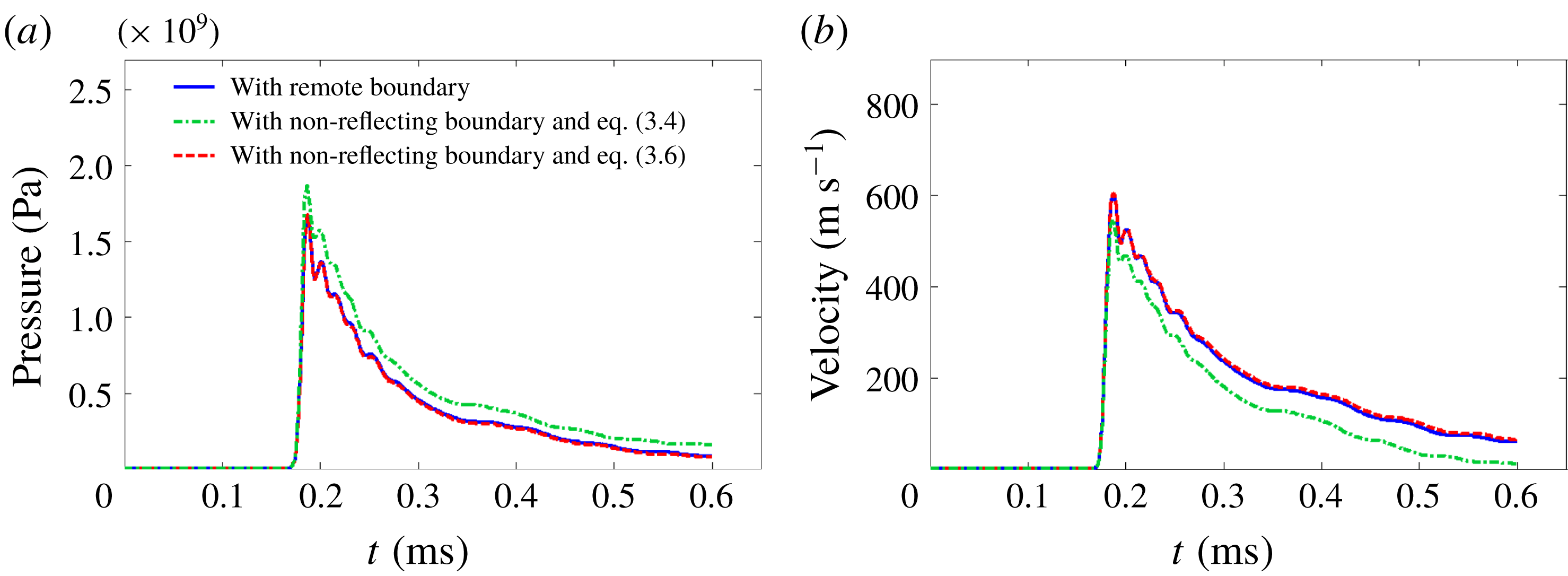
The time histories of the pressure and velocity for the measuring point with different boundary conditions are presented in figure 6. It can be seen that the value of
 $t_{B}$
has a substantial influence on the non-reflection effect. Both the velocity and pressure errors induced by the reflected waves are significant when (3.4) is adopted, while they become so small that they can be neglected when (3.6) is used, thus demonstrating that (3.6) leads to a more accurate estimation of
 $t_{B}$
.
One-dimensional underwater explosion: comparison of the time evolutions of the pressure (a) and velocity (b) at the measuring point between the result with the proposed non-reflecting boundary and the remote boundary.

3.3 Numerical tests and the influence of parameters
In this subsection, a 2-D underwater explosion is simulated to validate the proposed NRBC, and meanwhile, the influence of the position and the shape of the boundary on the non-reflection effect is investigated.
Underwater explosion is a critical issue posing a great threat to ship structures (Cui, Zhang & Wang Reference Cui, Zhang and Wang2016; Zhang et al. Reference Zhang, Wu, Liu and Wang2017). The SPH method has been proved to be a good algorithm to simulate underwater explosions which are featured by large deformations and material fragmentations (see e.g. Klaseboer et al. Reference Klaseboer, Hung, Wang, Wang, Khoo, Boyce, Debono and Charlier2005; Zhang, Yang & Yao Reference Zhang, Yang and Yao2012; Ming et al. Reference Ming, Zhang, Xue and Wang2016). However, if the computing domain is limited to a small region of interest with inappropriate boundary conditions imposed, the generated shock wave with pressure up to dozens of GPa will be reflected back into the interior, which often has a non-negligible impact on the prediction of the shock wave load, as well as the shape and motion of the bubble produced by the detonations (Liu et al. Reference Liu, Ming, Zhang, Miao and Liu2018).
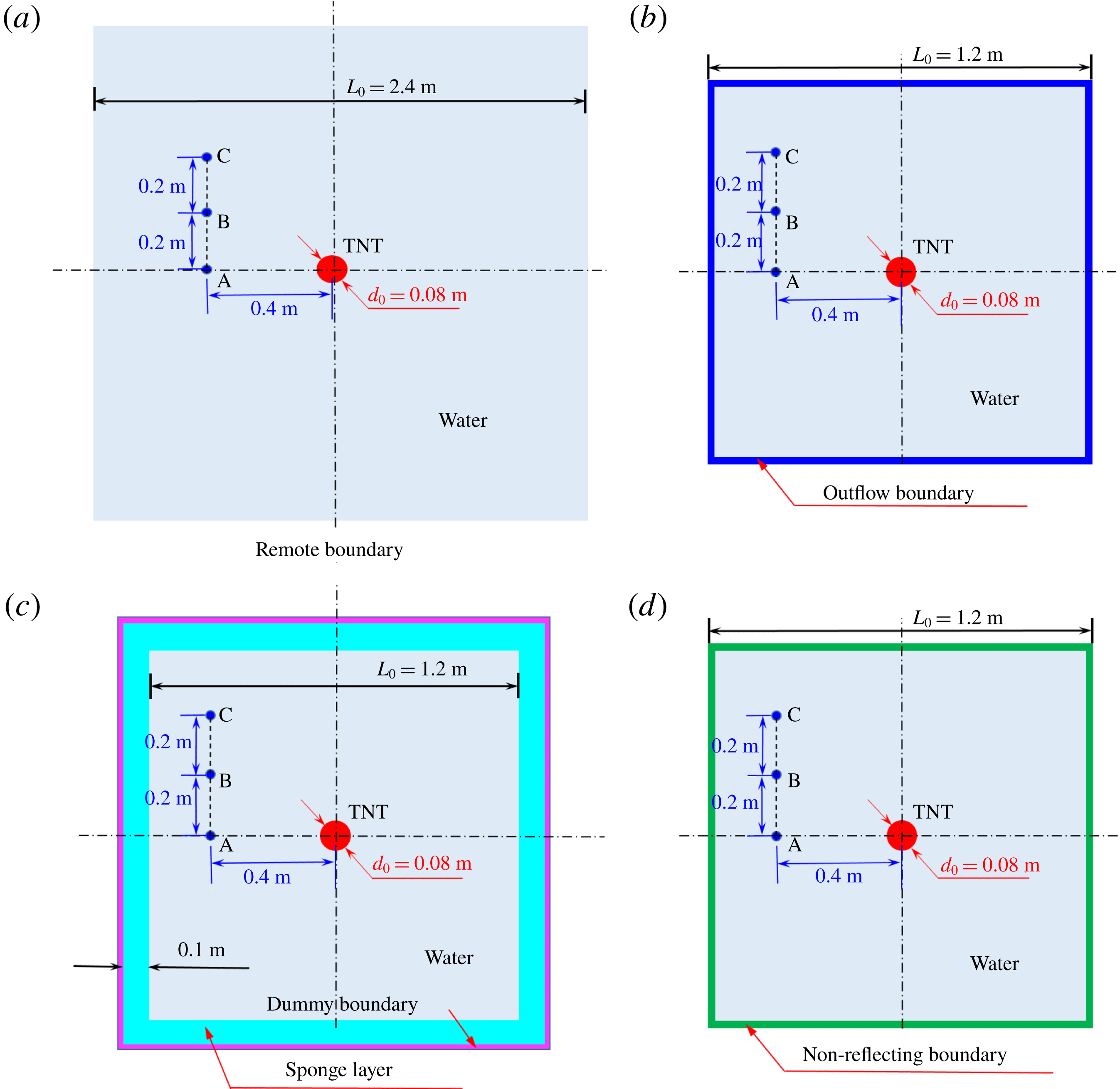
A sketch of the computational model with the proposed NRBC enforced is given in figure 7(d), where a circular TNT charge is located at the centre of a square water domain with four layers of boundary particles initially placed outside. The initial density and pressure of TNT are
 $1630~\text{kg}~\text{m}^{-3}$
and zero, respectively. Gravity is not taken into account. The charge is denoted at the centre. The duration of the whole simulation is 0.55 ms. For comparison, this simulation is repeated applying the outflow boundary proposed by Tafuni et al. (Reference Tafuni, Domínguez, Vacondio and Crespo2018) and the sponge layer introduced by Gong et al. (Reference Gong, Liu and Wang2009). The model with a larger square water domain of
 $2.4~\text{m}\times 2.4~\text{m}$
with no boundary condition enforced is selected as a reference solution. This model has the minimum water domain size that can ensure no shock waves produced by the detonation reach the boundary at the end of the simulation. The models of the above four cases are initialized through a Cartesian grid with an initial spatial resolution of 0.002 m. The initial sound speed
 $c_{0}$
and density
 $\unicode[STIX]{x1D70C}_{0}$
of water are
 $1480~\text{m}~\text{s}$
and
 $1000~\text{kg}~\text{m}^{-3}$
, respectively. There are three gauging points A, B and C in the water domain to record the pressure and velocity evolution, and their locations are shown in figure 7.
Two-dimensional underwater explosion. Sketches of the computational models with different boundary conditions. (a) The remote boundary condition, (b) the outflow boundary condition (Tafuni et al. Reference Tafuni, Domínguez, Vacondio and Crespo2018), (c) the sponge layer boundary condition (Gong et al. Reference Gong, Liu and Wang2009) and (d) the proposed NRBC.

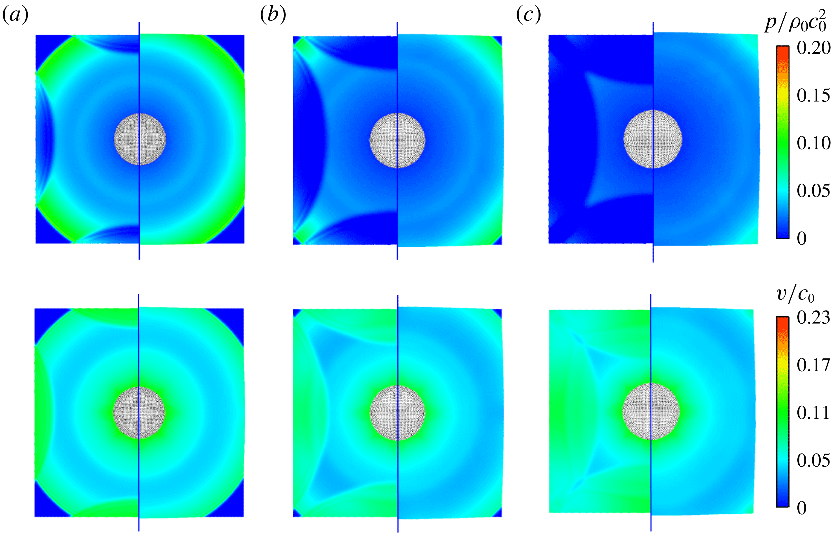
The pressure and velocity nephrograms of the water domain obtained by applying the outflow boundary condition (the left side) and the proposed NRBC (the right side) at three selected instants are shown in figure 8. It can be observed that with the detonation of the charge, there are cylindrical waves presented in both the pressure and velocity fields. When the outflow boundary condition is enforced, the rarefaction waves induced by the boundary are reflected back into the interior, resulting in low pressure regions and high-speed zones. For the case with the proposed NRBC, there is no obvious perturbation induced by the boundary in either the pressure or velocity field. The waves with different angles of incidence propagate through the boundaries freely just as they pass through the interior domain.
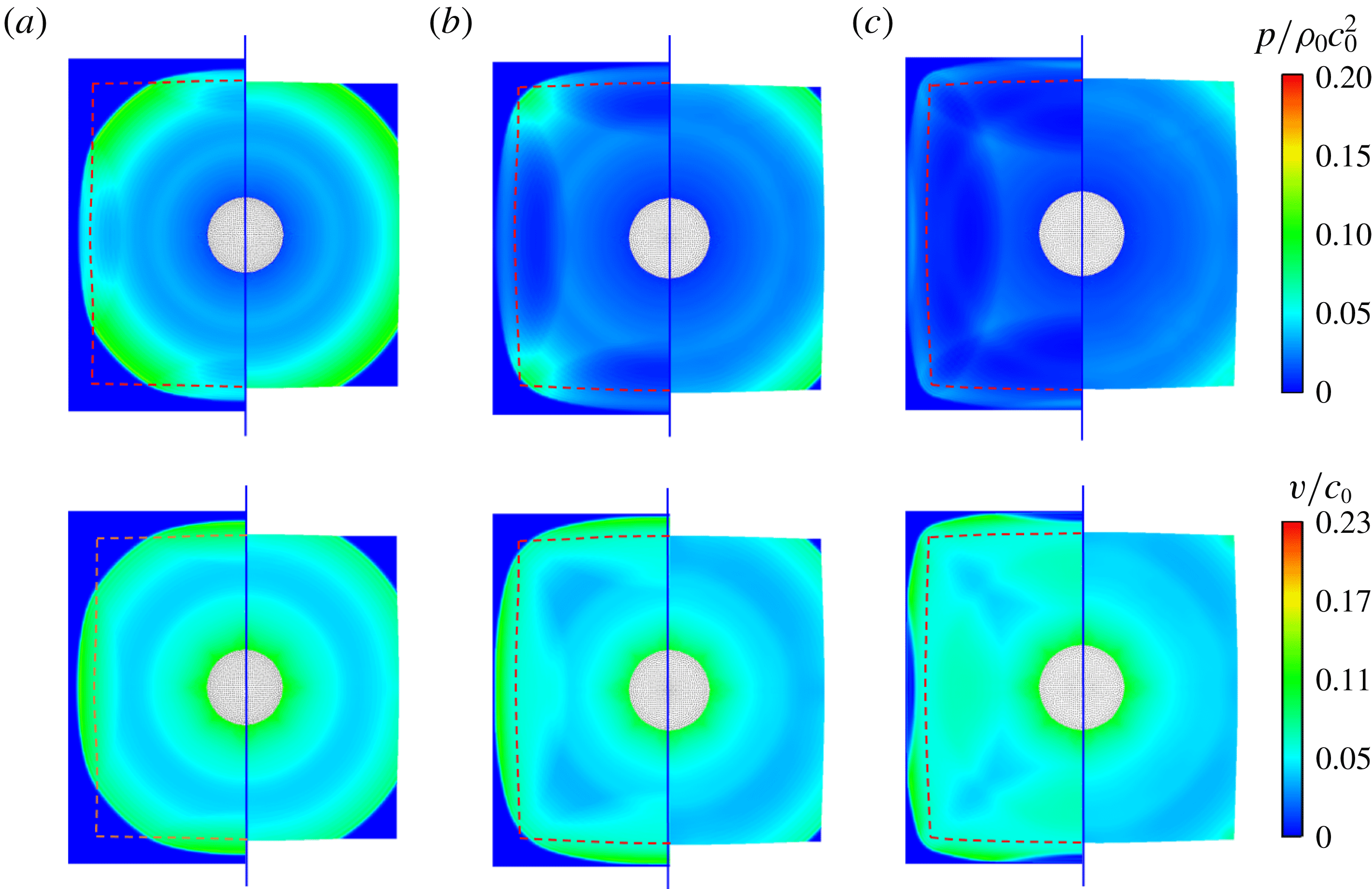
Similarly, the comparison between the sponge layer (the left side) and the proposed NRBC (the right side) is shown in figure 9, where the dashed line represents the interface between the sponge layer and the water domain. It can be observed that the sponge layer significantly slows down the propagation velocity of the waves, leading to an obvious change of the shape of the wave fronts. But the reflected waves are also apparent in both pressure and velocity fields.
Two-dimensional underwater explosion: snapshots of pressure (top row) and velocity (bottom row) fields of water with the outflow boundary introduced by Tafuni et al. (Reference Tafuni, Domínguez, Vacondio and Crespo2018) (the left side), compared with the solution with the proposed non-reflecting boundary (the right side) at three instants (a)
 $tc_{0}/L_{0}=0.42$
; (b)
 $tc_{0}/L_{0}=0.49$
; (c)
 $tc_{0}/L_{0}=0.57$
.

Two-dimensional underwater explosion: snapshots of pressure (top row) and velocity (bottom row) fields of water with the sponge layer introduced by Gong et al. (Reference Gong, Liu and Wang2009) (the left side), compared with the solution with non-reflecting boundary (the right side) at three instants (a)
 $tc_{0}/L_{0}=0.42$
; (b)
 $tc_{0}/L_{0}=0.49$
; (c)
 $tc_{0}/L_{0}=0.57$
. The dashed line indicates the interface between the sponge layer and the water domain.

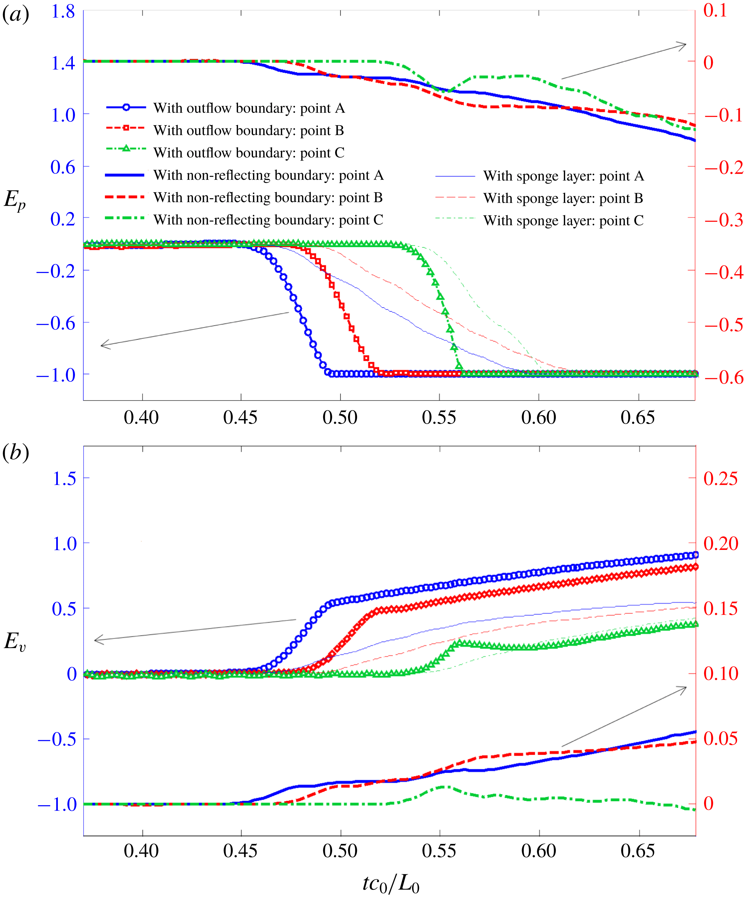
The quantitative comparisons of the time evolutions of the relative errors of the pressure and velocity of gauging points A, B and C are presented in figure 10. For the velocity, here the direction from the detonation point to the measuring points is taken as positive. The relative errors at different times caused by the application of the NRBC, the outflow boundary condition and the sponge layer boundary condition are defined as
 $$\begin{eqnarray}E_{q}(t)=\frac{q(t)-\bar{q}(t)}{\bar{q}(t)}\quad \text{with}~q(t)\in \{p(t),v(t)\},\end{eqnarray}$$
where
 $\bar{q}(t)$
denotes the pressure and velocity at time
 $t$
obtained by using the remote boundary condition while
 $q(t)$
is the corresponding variable values yielded by enforcing the NRBC, the outflow boundary condition and the sponge layer boundary condition.
From figure 10 we can observe that, for the same measuring point, the relative errors of pressure and velocity appear at approximately the same time, even though the applied boundary conditions are different. Further, as the distance between the measuring points and the detonation point increases, which implies a increase of the propagation distance of the incident shock waves produced by the detonation, both the pressure and velocity errors occur later. For the cases with the outflow boundary and the sponge layer, the relative errors of pressure and velocity increase rapidly after the reflected waves arrive. In particular, the relative errors of pressure eventually tent to be constant
 $-1$
for all gauging points. This is attributed to the adoption of the cutoff model presented in § 2.3. In this cutoff model, the minimum pressure of the measuring points is prescribed to be 0, and thus the corresponding maximum pressure error is
 $-1$
. Regarding the result with NRBC, the relative errors of pressure and velocity for all the measuring points with different incident angles are significantly reduced to less than 15 % and 10 %, respectively, which further validates the applicability and accuracy of the proposed NRBC for underwater explosions.
Two-dimensional underwater explosion: time evolutions of the relative errors of pressure (a) and velocity (b) of gauging points obtained by applying the outflow boundary condition (Tafuni et al. Reference Tafuni, Domínguez, Vacondio and Crespo2018), the sponge layer boundary condition (Gong et al. Reference Gong, Liu and Wang2009) and the proposed NRBC. The result applying the remote boundary is selected as the reference solution. The outflow boundary condition and the sponge layer boundary condition are plotted on the left axis while the NRBC is on the right axis.

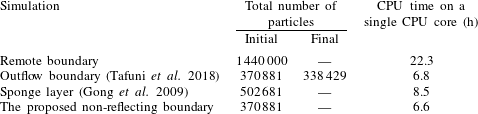
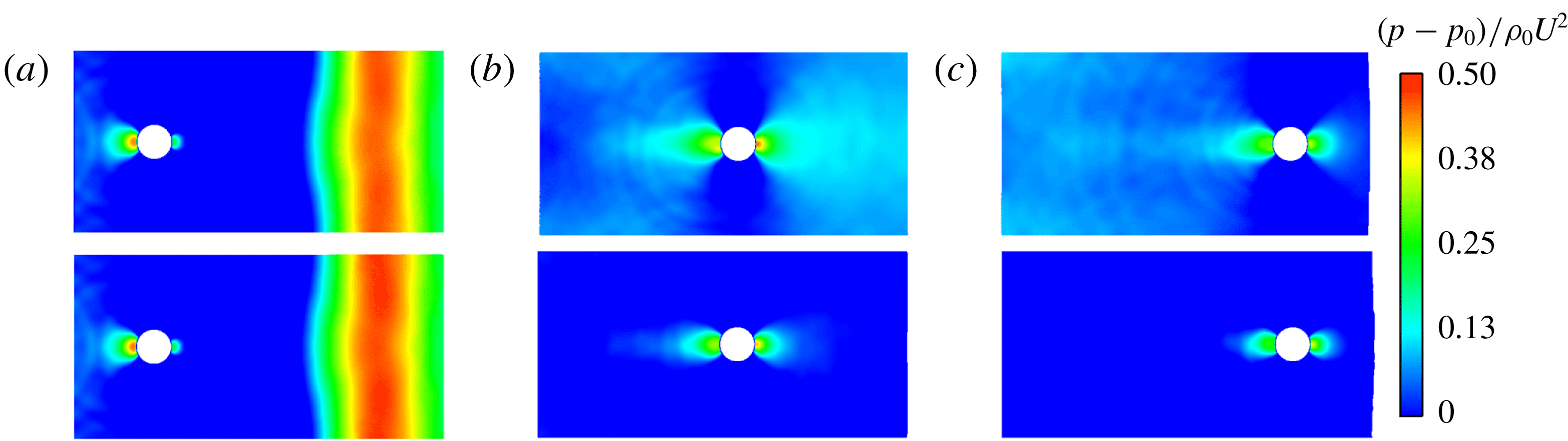
To verify the efficiency of the proposed NRBC, the comparisons of total number of particles and CPU time for the four models applying different boundary conditions are given in table 3. All these simulations ran on a machine equipped with a quad-core processor of i7-4790 with a frequency of 3.60 GHz. Note that, for the case with the outflow boundary condition, the total number of particles decreases over time owing to the deletion of particles, while for the other three cases, the particle number remains constant during the whole simulation process. The cases with the outflow boundary condition and the NRBC have same initial particle numbers and CPU time, which are obviously less than other two cases, demonstrating the efficiency of these two boundary conditions. The initial particle number of the case with the remote boundary is approximately four times those of the outflow boundary condition and the NRBC. As a result, the required CPU time of the remote boundary increases significantly with respect to other two cases. Similarly, the enforcement of the sponge layer also brings about a remarkable increase in the number of particles and, therefore, the CPU time increases significantly. For the cases with the outflow boundary condition and the present NRBC, the required number of particles and CPU time are close. But the present NRBC can more accurately guarantee the pressure and velocity non-reflection in both low- and high-speed problems.
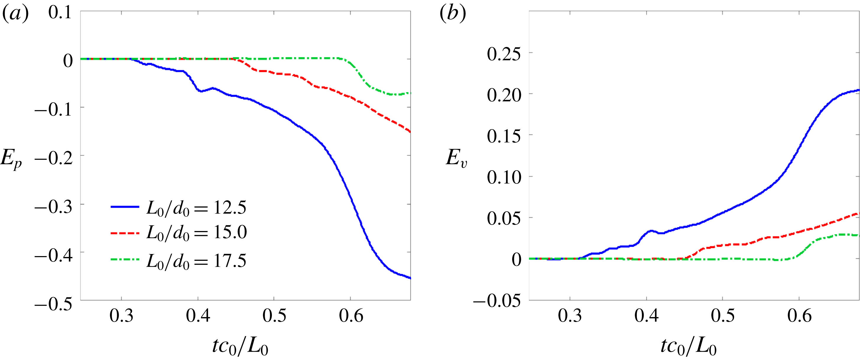
Two-dimensional underwater explosion applying the proposed NRBC: time evolutions of relative errors of pressure (a) and velocity (b) at measuring point A with different sizes of water domain.
 $L_{0}$
denotes the initial side length of the square water domain, and
 $d_{0}$
is the initial diameter of the TNT charge.

Comparisons of total number of particles and CPU time for the cases of 2-D underwater explosions with different boundary conditions.

Subsequently, to assess the influence of the distance between the pressure source and the boundary on the non-reflection effect of the proposed NRBC, the initial side length of the square water domain
 $L_{0}$
is set to
 $12.5d_{0}$
,
 $15.0d_{0}$
and
 $17.5d_{0}$
, respectively, where
 $d_{0}=0.08~\text{m}$
is the initial diameter of the TNT charge. For these three models, the time evolutions of the pressure and velocity relative errors at the measuring point A are displayed in figure 11. The reference solution is still the result with the remote boundary. It can be concluded that the further the boundary is from the measuring point, the less is the error with respect to the reference solution. In particular, when the side length is approximately 17.5 times the diameter, the relative errors of the pressure and velocity are within 10 % and 5 %, respectively. As a consequence, one should note that the proposed NRBC is only approximate, and should be placed as far as possible from the region of interest.
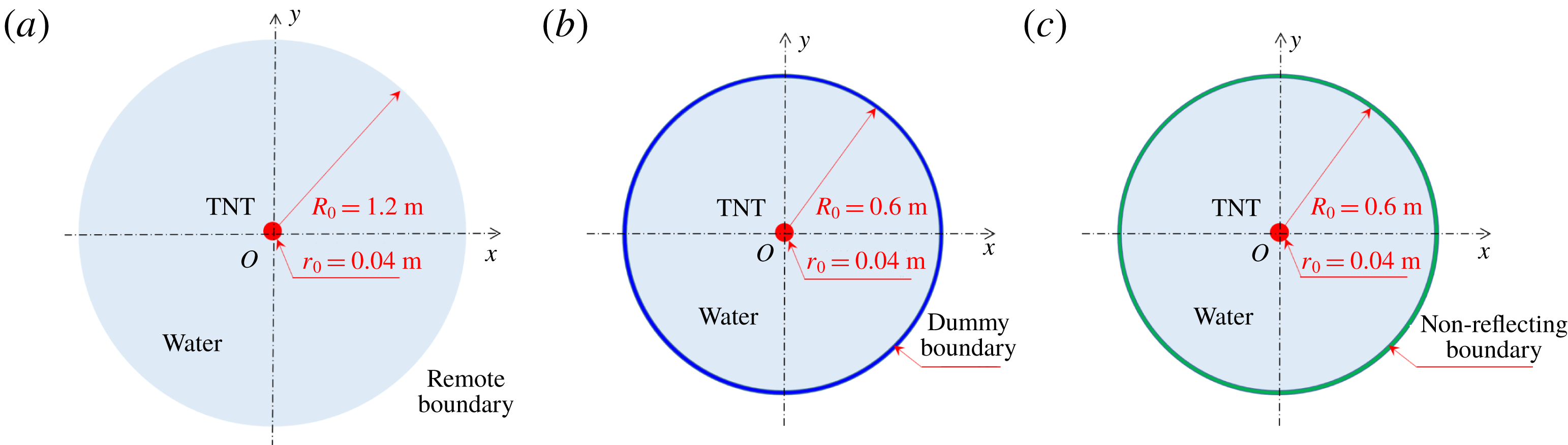
The previous numerical tests have shown the validity of the proposed NRBC in dealing with straight boundaries. Here, we also perform a 2-D underwater explosion but adopt circular water domains to check the applicability of this NRBC for curved boundaries. Three computational models applying different boundary conditions are established, as sketched in figure 12. For these models, the particles are initially placed on a series of concentric circles with the same spacing 0.002 m.
Two-dimensional underwater explosion with a circular water domain. Sketches of the models with the remote boundary (a), the dummy boundary (b) and the proposed non-reflecting boundary (c). For these three models, the particles are initially placed on a series of concentric circles with the same spacing 0.002 m.

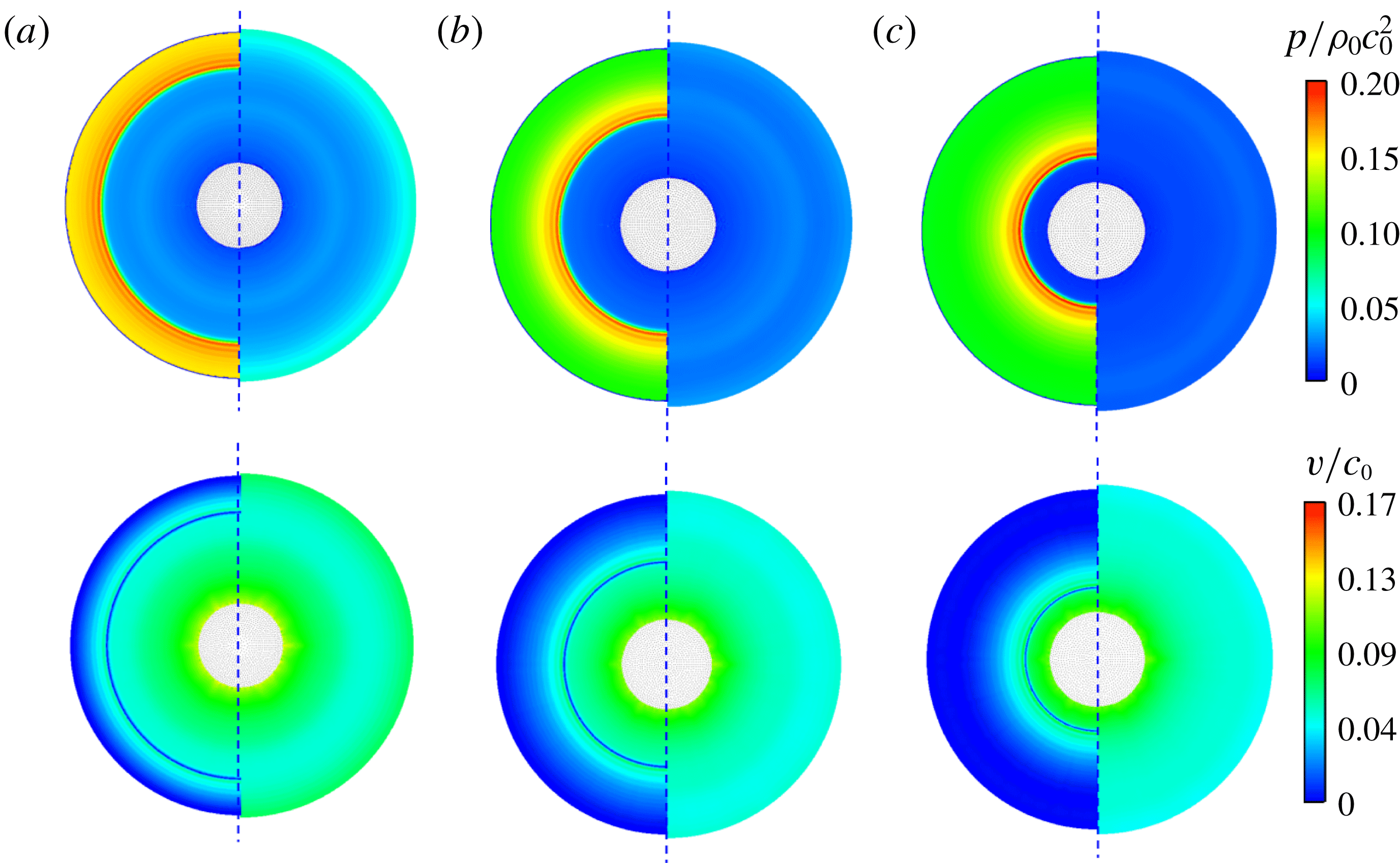
Two-dimensional underwater explosion with a circular water domain. The pressure (top row) and velocity (bottom row) profiles of the water domain at three instants after the shock wave reaches the boundary, (a)
 $tc_{0}/R_{0}=0.84$
; (b)
 $tc_{0}/R_{0}=0.98$
; (c)
 $tc_{0}/R_{0}=1.14$
. Left: dummy boundary (Adami et al. (Reference Adami, Hu and Adams2012)). Right: the proposed non-reflecting boundary.

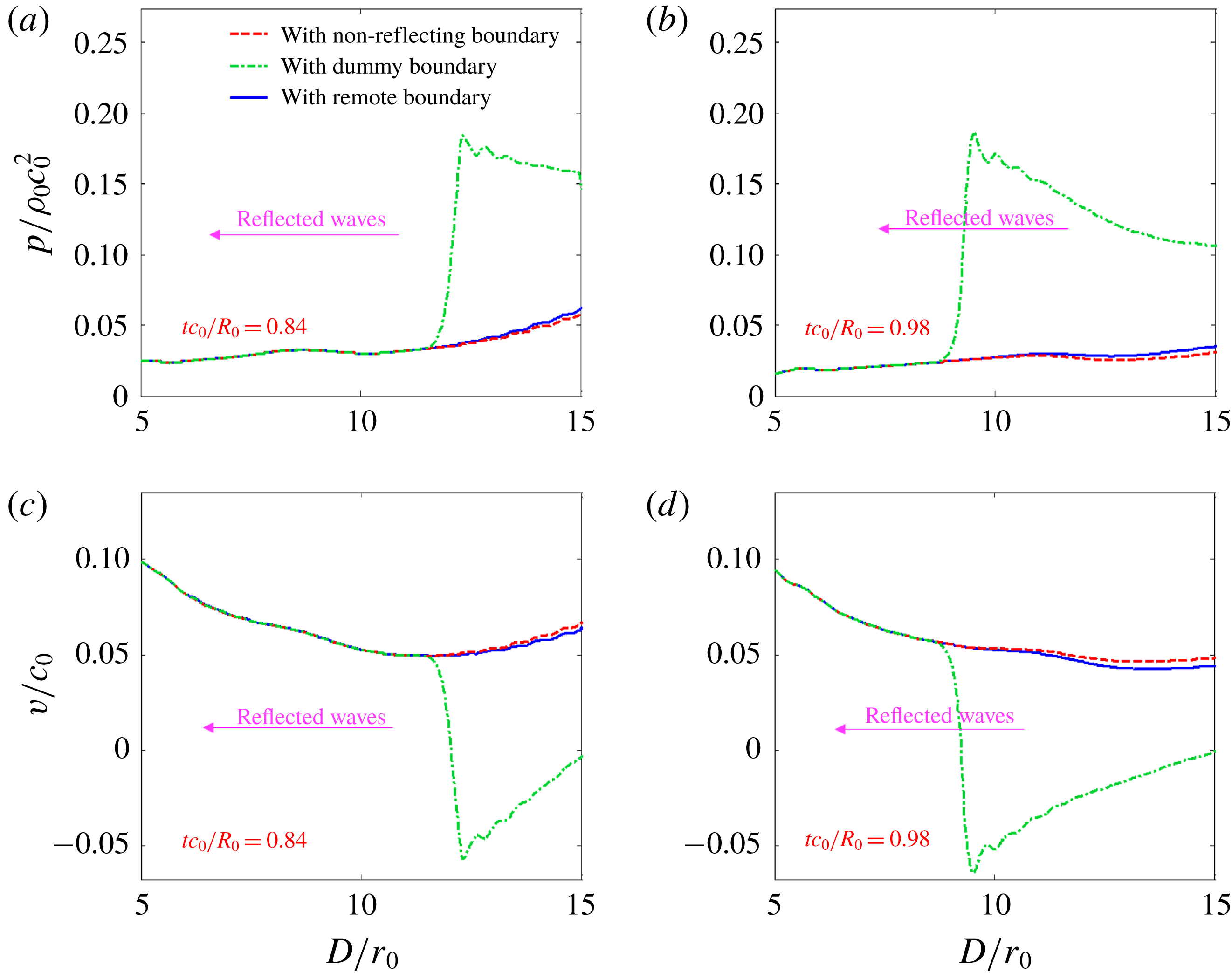
The pressure and velocity fields of the water domain with the dummy boundary (the left side) and the non-reflecting boundary (the right side) at three instants after the shock wave arrives at the boundary are presented in figure 13. When the dummy boundary condition is imposed, strong reflected waves propagate from the boundary to the interior, while these reflections become much weaker when the NRBC is enforced. These behaviours can also be proved by the pressure and velocity spatial distributions along the
 $x$
axis at two instants, as shown in figure 14, where the variable
 $D$
denotes the distance between the measuring points and the detonation point non-dimensionalized with the initial radius of the explosive
 $r_{0}$
. As expected, for the case with the dummy boundary, there is a large amplitude pressure wave propagating from the boundary to the interior, which reduces the velocity of the particles and even reverses their direction. In contrast, despite the weak rarefaction wave produced by the NRBC, the errors of pressure and velocity are both reduced significantly. In other words, the proposed NRBC is demonstrated to be applicable to curved boundaries.
Two-dimensional underwater explosion with a circular water domain. The pressure (top) and velocity (bottom) distributions along the
 $x$
axis with the dummy boundary (Adami et al.
Reference Adami, Hu and Adams2012) and the proposed non-reflecting boundary, compared with the remote boundary. The variable
 $D$
, denoting the distance between the measuring point and the detonation point, is non-dimensionalized with the initial radius of explosive
 $r_{0}$
.

4 Examples
In this section, several numerical examples of fluid dynamics including water flows and underwater explosions are presented to demonstrate the accuracy and reliability of the proposed NRBC. Firstly, the water entry of a free-falling wedge is simulated to verify the accuracy of the NRBC for common impact problems with a free surface. Then, the simulation of a moving circular cylinder inside a rectangular box is conducted to demonstrate that the NRBC is applicable for low-speed flows. The last case concerns a 3-D underwater explosion, aiming to prove that the proposed NRBC can be applied to three-dimensional problems.
4.1 Two-dimensional water entry of a free-falling wedge
In this part, the simulation of two-dimensional water entry of a free-falling wedge is carried out to validate the NRBC. According to the experiment of Zhao & Faltinsen (Reference Zhao and Faltinsen1993), the width of the triangle base is
 $L=0.5~\text{m}$
, and the deadrise angle is
 $30^{\circ }$
. The mass of the wedge is 241.0 kg. At the initial moment, the wedge impacts on the water with an initial speed of
 $v_{0}=6.15~\text{m}~\text{s}^{-1}$
. In this simulation, gravity
 $\boldsymbol{g}=9.8~\text{m}~\text{s}^{-2}$
is taken into account with its direction vertically downward. In the present SPH scheme, the problem is simplified to two dimensions, and the wedge is treated as moving dummy boundaries discretized into four layers of particles. Firstly, the
 $\unicode[STIX]{x1D6FF}$
-SPH scheme is validated by comparing with the measurements, and the convergence is studied by setting three different particle resolutions:
 $L/\unicode[STIX]{x0394}x=125$
,
 $L/\unicode[STIX]{x0394}x=250$
and
 $L/\unicode[STIX]{x0394}x=500$
, where
 $\unicode[STIX]{x0394}x$
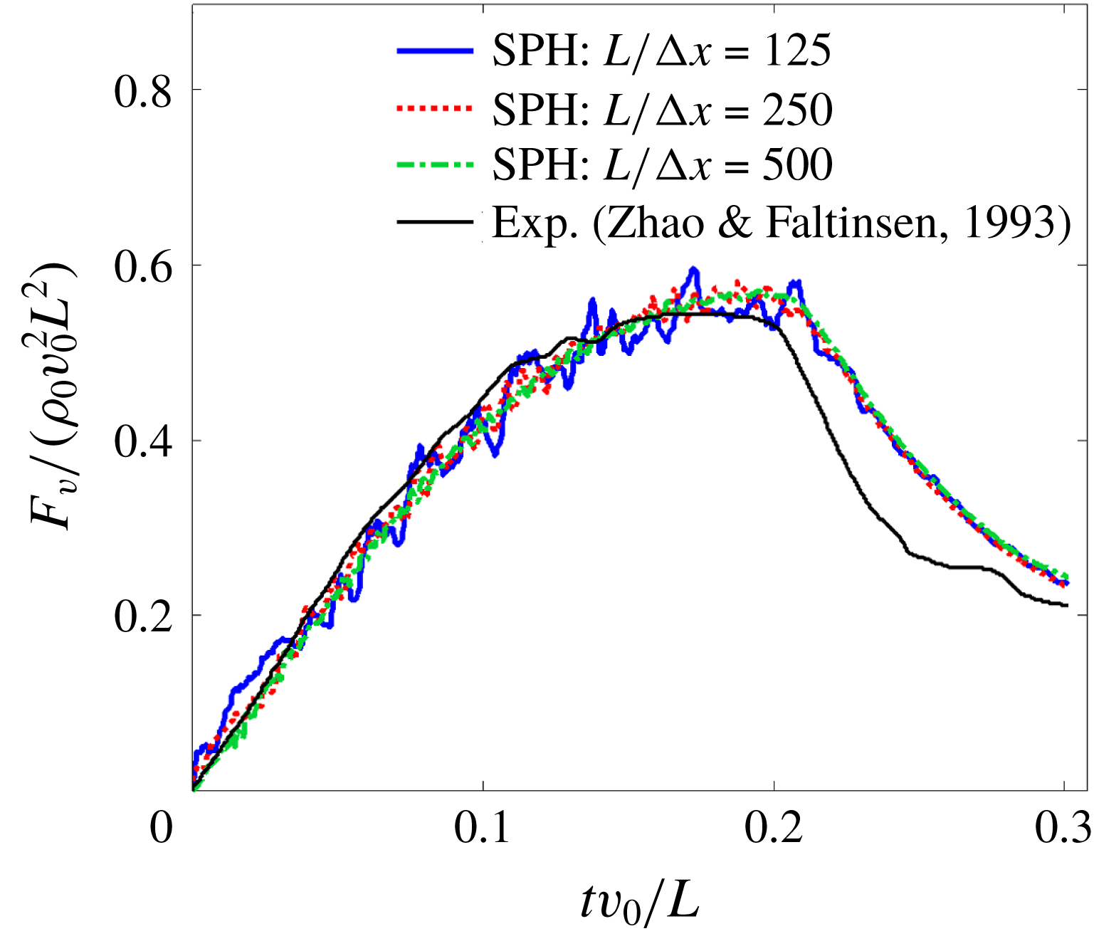
is the initial particle spacing. To avoid the wave reflection induced by the boundary, the width and depth of the water area are set to 4.0 m and 2.0 m, respectively, which can ensure that the pressure waves produced by the impact have not reached the boundary by the end of the simulation. In figure 15, the time history of the non-dimensional total vertical force acting on the wedge is presented, and compared with the measurements.
 $F_{v}$
denotes the vertical force and
 $\unicode[STIX]{x1D70C}_{0}=1000~\text{kg}~\text{m}^{-3}$
is the initial density of water. It can be seen that, with an increase in resolution, the numerical results converge to the experimental data. However, the vertical force is over-predicted at the later stage due to the three-dimensional effect, as mentioned by Zhao & Faltinsen (Reference Zhao and Faltinsen1993). In general, the numerical outcome can be regarded as agreeing well with the experimental data, thus validating the accuracy of the SPH model applied in the present work.
Two-dimensional water entry of a free-falling wedge. Time histories of the vertical force for different resolutions, compared with the experimental data in Zhao & Faltinsen (Reference Zhao and Faltinsen1993). The size of the water domain is
 $4.0~\text{m}\times 2.0~\text{m}$
with no boundary conditions imposed.

Subsequently, to check the accuracy of the proposed NRBC, the water entry of the wedge in a reduced water domain with the NRBC enforced is simulated, and compared with the results obtained by enforcing the outflow boundary condition (Tafuni et al.
Reference Tafuni, Domínguez, Vacondio and Crespo2018) and the sponge layer boundary condition (Gong et al.
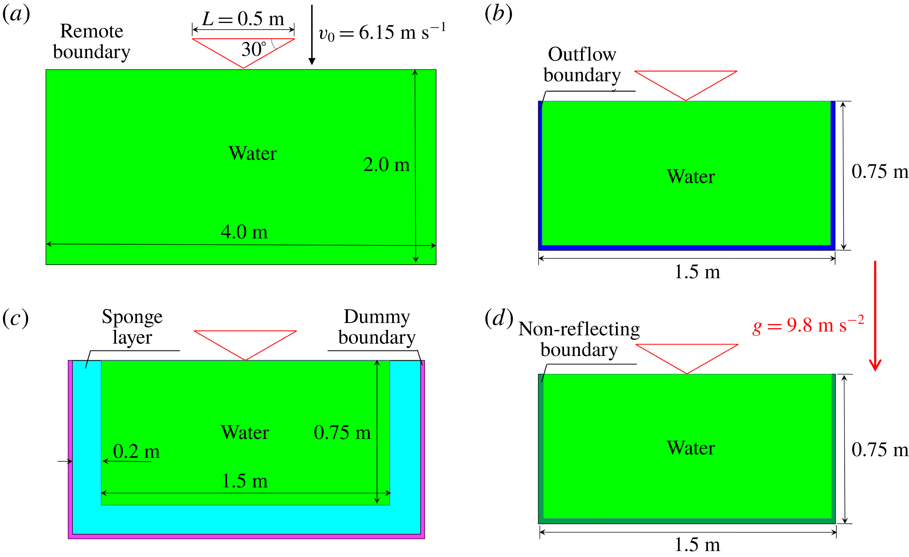
Reference Gong, Liu and Wang2009). For these three cases, the size of the water domain is reduced to 1.5 m long and 0.75 m deep. The thickness of the sponge layer is set to 0.2 m. Additionally, the result with the remote boundary is used to provide an exact reference solution. For all of these four cases, the particle resolution is
 $L/\unicode[STIX]{x0394}x=500$
, and the computational models are displayed in figure 16.
Two-dimensional water entry of a free-falling wedge. Sketches of the calculation models with the different boundary conditions. (a) The remote boundary condition; (b) the outflow boundary condition (Tafuni et al. Reference Tafuni, Domínguez, Vacondio and Crespo2018); (c) the sponge layer boundary condition (Gong et al. Reference Gong, Liu and Wang2009); and (d) the proposed NRBC.

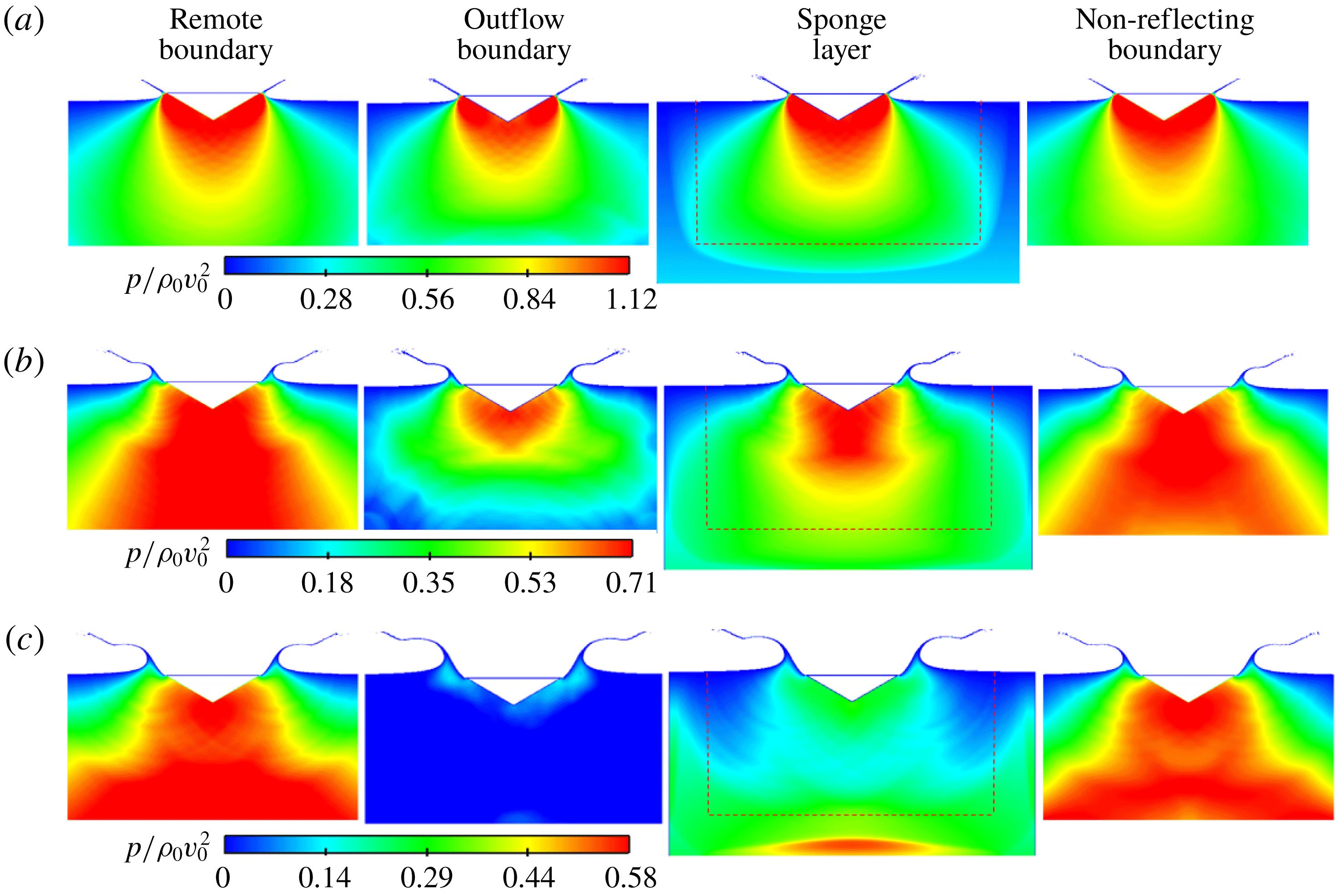
In figure 17, the pressure field evolution with the outflow boundary, the sponge layer and the proposed non-reflecting boundary are displayed, and compared with the result with the remote boundary. It is worth noting that, for the case with the remote boundary, only part of the whole water domain, whose size is identical to the water domain of other cases, is displayed. It can be seen that when the outflow boundary is enforced, the rarefaction waves induced by the boundary are apparent and the pressure field becomes asymmetric. For the results with the sponge layer, it can be observed that, after the pressure wave reaches the sponge layer, there is a sudden decrease in its propagation velocity, leading to a very different pressure distribution from that with the remote boundary. At
 $tv_{0}/L=0.295$
, the rarefaction waves produced by the sponge layer reach the wedge and the pressure field is altered significantly. Afterward, the pressure waves travel through the sponge layer and reach the outermost dummy boundary, reflecting strong compression waves back to the interior domain. Regarding the case with the NRBC, before
 $tv_{0}/L=0.295$
, there is no significant pressure reflection occurring from the boundary, and the pressure field is very similar to that with the remote boundary. After that, the reflection is enhanced gradually along with the accumulation of error. Nonetheless, the reflected waves are much weaker with respect to those produced by the outflow boundary and the sponge layer.
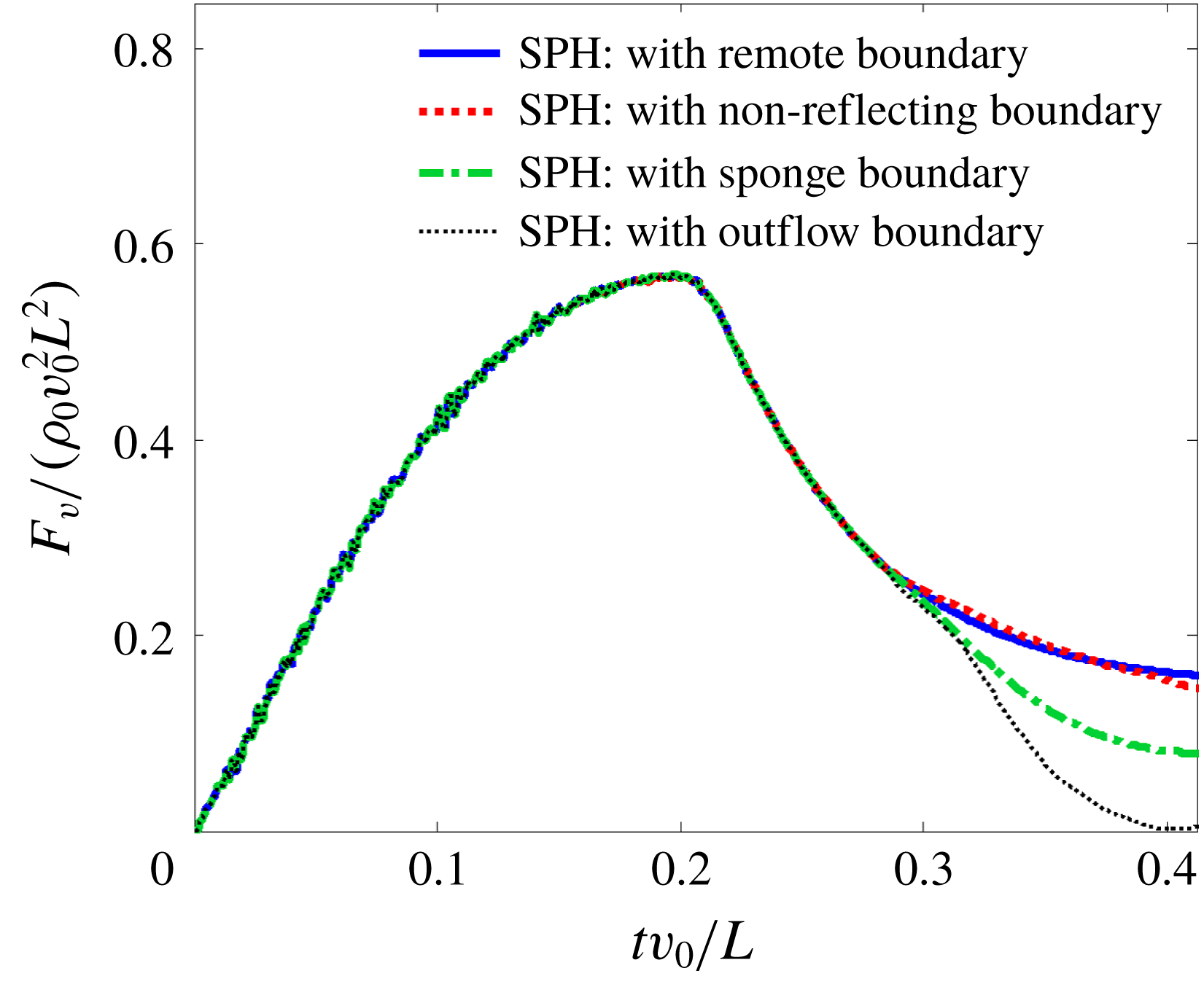
Figure 18 depicts the time histories of the vertical force obtained by applying different boundary conditions. The boundary conditions from left to right are the remote boundary, the outflow boundary, the sponge layer and the non-reflecting boundary, respectively. The dashed line represents the interface between the sponge layer and water domain. It can be observed that, before approximately
 $tv_{0}/L=0.3$
, the vertical force obtained by applying the outflow boundary and the sponge layer coincide with that of the remote boundary, even though the pressure field has been significantly affected by the reflected waves. The reason is that the reflected waves do not reach the wedge before approximately
 $tv_{0}/L=0.3$
. In the later stage, the vertical force for the cases with the outflow boundary and the sponge layer is underestimated due to the reflected waves interacting with the wedge. Regarding the case with the NRBC, the curve agrees well with that with the remote boundary condition, which is equivalent to little pressure reflection, thus further demonstrating the accuracy of the proposed NRBC.
Water entry of a free-falling wedge. Pressure field obtained by enforcing different boundary conditions at three different time instants: (a)
 $tv_{0}/L=0.221$
; (b)
 $tv_{0}/L=0.295$
; (c)
 $tv_{0}/L=0.369$
. The boundary conditions from left to right are the remote boundary, the outflow boundary (Tafuni et al.
Reference Tafuni, Domínguez, Vacondio and Crespo2018), the sponge layer (Gong et al.
Reference Gong, Liu and Wang2009) and the proposed non-reflecting boundary, respectively. The dashed line represents the interface between the sponge layer and the water domain.

Water entry of a free-falling wedge. Time histories of the vertical force obtained by applying the outflow boundary (Tafuni et al. Reference Tafuni, Domínguez, Vacondio and Crespo2018), the sponge layer (Gong et al. Reference Gong, Liu and Wang2009), the proposed non-reflecting boundary and the remote boundary.

4.2 Two-dimensional flow around a moving cylinder in rectangular domain
The second problem considered is the two-dimensional flow around a moving circular cylinder in a rectangular box. As studied in Marrone et al. (Reference Marrone, Colagrossi, Antuono, Colicchio and Graziani2013), the sudden movement of the cylinder radiates pressure waves in a weakly compressible fluid, and when the solid boundary condition is applied, the spurious reflected waves tend to cause unphysical disturbances on the drag force that acts upon the cylinder. However, in the present work, the non-reflecting boundary can help to tackle this problem.
Firstly, to illustrate the unphysical pressure reflection problem, and meanwhile, to check the accuracy and convergence of the present procedure, this flow is simulated by using the
 $\unicode[STIX]{x1D6FF}$
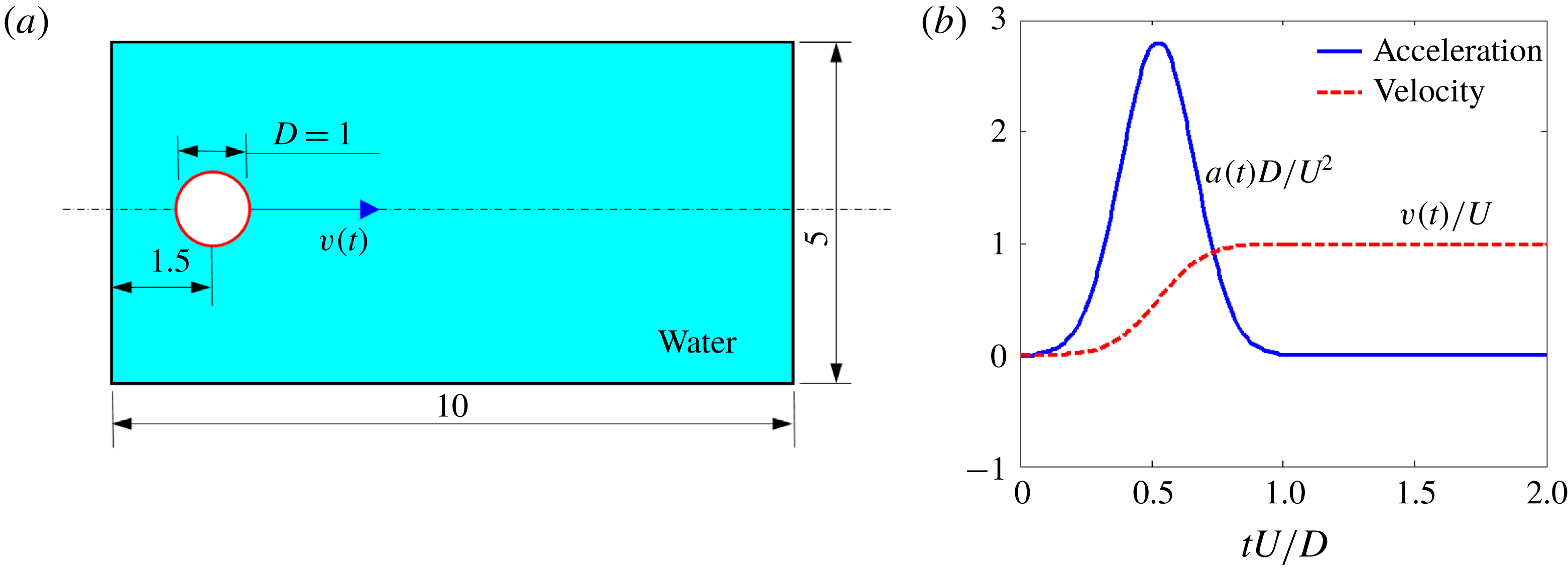
-SPH method with the dummy boundary condition imposed around the water domain. The sketch of the whole model is illustrated in figure 19(a). During the time interval
 $tU/D\in [0,1]$
, the cylinder accelerates along the
 $x$
-axis until it attains a speed of
 $U$
. Its acceleration and velocity are prescribed by the curves displayed in figure 19(b). In this test, the physical viscosity of water is not considered, but artificial viscous is taken into account for good numerical stability. In addition, to eliminate the unphysical cavitation in the water domain induced by the tensile instability, the background pressure
 $p_{0}=3\unicode[STIX]{x1D70C}_{0}U^{2}$
provided by Marrone et al. (Reference Marrone, Colagrossi, Antuono, Colicchio and Graziani2013) is applied. By using the particle packing algorithm introduced by Colagrossi et al. (Reference Colagrossi, Bouscasse, Antuono and Marrone2012), a regular particle distribution close to the cylinder at the preprocessing stage is obtained. Gravity is not considered in this simulation.
A moving circular cylinder in a rectangular box. The sketch of the whole model (a) and the time evolution of the circular cylinder motion (b), refer to Marrone et al. (Reference Marrone, Colagrossi, Antuono, Colicchio and Graziani2013).

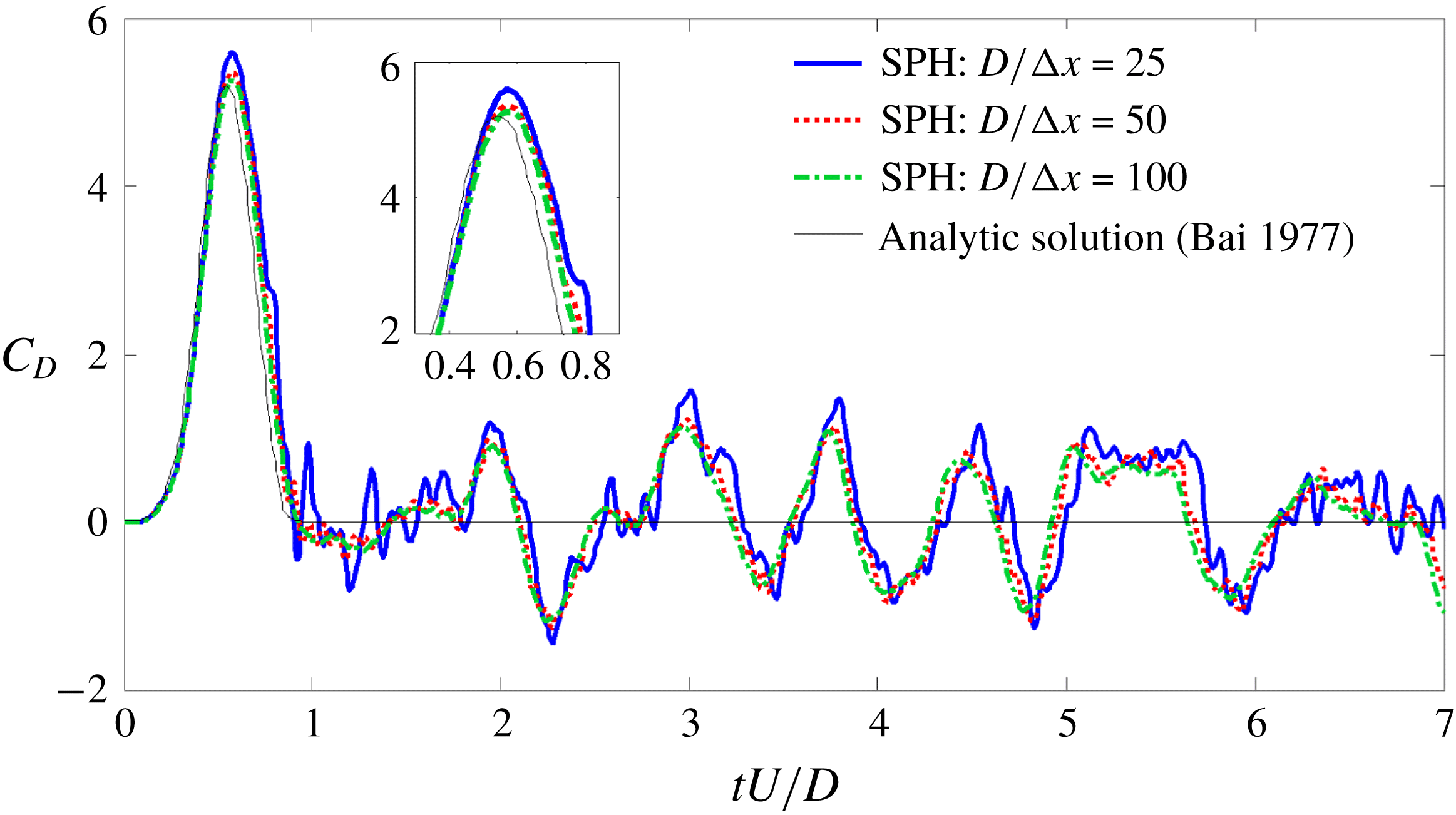
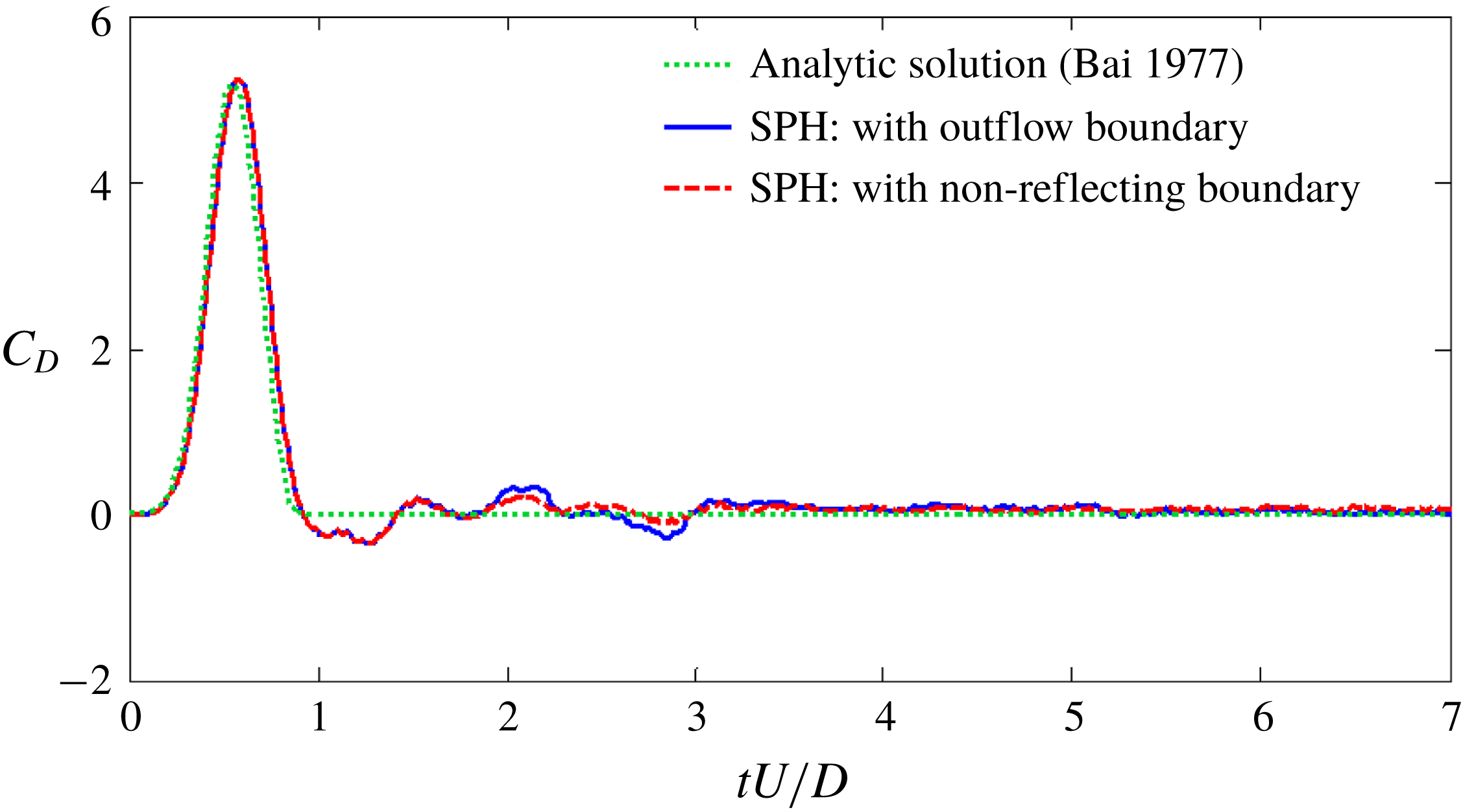
Time histories of the drag coefficient with three different particle resolutions are shown in figure 20, compared with the analytical solution provided by Bai (Reference Bai1977) for incompressible potential flow. The drag coefficient is defined as
 $C_{D}=2F_{x}/\unicode[STIX]{x1D70C}U^{2}D$
, where
 $F_{x}$
and
 $D$
denote the resistance along the
 $x$
axis and the diameter of the cylinder, respectively. From figure 20, the SPH algorithm applied in the present work has a good performance in terms of convergence. During the time interval
 $tU/D\in [0,1]$
, the magnitude of the drag force increases to the peak value and then decreases to approximately 0. Note that there is a slight difference between the SPH solution and the analytical result in the phase and amplitude of the first peak owing to the influence of the weak compressibility, more details can be found in Marrone et al. (Reference Marrone, Colagrossi, Antuono, Colicchio and Graziani2013). However, after
 $tU/D=1.0$
, when the steady state is reached, the curves obtained by using the SPH method are characterized by large amplitude oscillations due to the reflected waves interacting with the cylinder.
A moving circular cylinder in a rectangular box. Time evolutions of the drag coefficient acting on the cylinder obtained with the SPH method with three different resolutions when a dummy boundary (Adami et al. Reference Adami, Hu and Adams2012) is enforced around the water domain, compared with the analytical solution provided by Bai (Reference Bai1977).

Then, to reduce the unphysical pressure reflection, the outflow boundary condition introduced by Tafuni et al. (Reference Tafuni, Domínguez, Vacondio and Crespo2018) and the proposed NRBC are respectively assigned to the right side of the boundary where the pressure waves are mainly reflected, while other three sides remain dummy boundary conditions to reduce the computational costs. For the entire model, the initial particle spacing and the smoothing length are set equal to 0.01 and 0.012, respectively. Figure 21 shows the pressure distribution at three time instants. The solution in the top row is obtained by applying the outflow boundary condition while the bottom row using the NRBC. The pressure wave, which can be approximated as a plane wave, is generated along with the accelerating movement of the cylinder. When the outflow boundary is arranged, some weak reflected waves can be observed in the pressure field. Regarding the result with the non-reflecting boundary, the pressure waves pass through the boundary freely with less reflection and the pressure field is smoother.
Figure 22 depicts time evolutions of the drag coefficient for these two boundary conditions. It can be observed that when the outflow boundary condition or the present NRBC is enforced, the unphysical oscillations of the drag force after
 $tU/L=1.0$
are reduced significantly. Overall, the present NRBC has a good performance in reducing the reflected waves for 2D low-speed flow problems.
A moving circular cylinder in a rectangular box. Comparison of the predicted pressure field between the result with the outflow boundary condition (Tafuni et al.
Reference Tafuni, Domínguez, Vacondio and Crespo2018) (top) and the solution with the proposed NRBC (bottom) enforced on the right side of the water domain at (a)
 $tU/D=1.2$
, (b)
 $tU/D=4.5$
, (c)
 $tU/D=7.0$
.

A moving circular cylinder in a rectangular box. Time histories of the drag coefficient obtained by using the SPH method with the outflow boundary condition (Tafuni et al. Reference Tafuni, Domínguez, Vacondio and Crespo2018) and the proposed NRBC, compared with the analytical solution in Bai (Reference Bai1977).

4.3 Three-dimensional underwater explosion
The numerical tests presented in § 3.3 have validated the NRBC for the two-dimensional underwater explosion. In this subsection, the underwater explosion simulation is extended to three-dimensional cases, aiming to show the applicability of the NRBC to three-dimensional problems.
Firstly, the simulation of underwater explosion in a free field is performed to validate the SPH procedure in the prediction of shock wave load. The whole computational model is sketched in figure 23(a), in which a spherical TNT charge with a radius
 $r_{0}=0.018~\text{m}$
is located at the central point of a cubical water region. The initial density and pressure of TNT are
 $1630~\text{kg}~\text{m}^{-3}$
and zero, respectively, and the charge is denoted at the centre. Gravity is not taken into account. The initial particle spacing
 $\unicode[STIX]{x0394}x$
and the smoothing length
 $h$
are respectively set to 0.002 m and 0.0024 m. In underwater explosions, the velocities of detonation and shock propagation are so rapid that the explosive gas and water can be assumed to be inviscid, and the whole process is adiabatic (Liu & Liu Reference Liu and Liu2003). There are two measuring points in the water domain and the distances between them and the charge centre are equal to 0.108 m and 0.144 m (i.e.
 $6.0r_{0}$
and
 $8.0r_{0}$
), respectively.
Three-dimensional free-field underwater explosion. (a) Sketch of the model. (b) Comparison of the pressure evolution at different detonation distances between the SPH method and the empirical data in Zamyshlyaev & Yakovlev (Reference Zamyshlyaev and Yakovlev1973).

In figure 23(b), the numerical result is compared with the empirical formula introduced by Zamyshlyaev & Yakovlev (Reference Zamyshlyaev and Yakovlev1973), where
 $d$
denotes the distance between the gauging points and the detonation point. It can be observed that the pressure–time curves obtained by using the SPH method agree well with the empirical data in the overall trend and peaks. However, some oscillations can be found in the numerical results, which may be because the SPH method adopted cannot cope well with the strong discontinuity induced by the shock wave (Wang et al.
Reference Wang, Zhang, Yu, Li and Kong2014). Indeed, this behaviour can also be observed in other numerical methods of discretization type (see e.g. Liu et al.
Reference Liu, Liu, Lam and Zong2003; Kim & Shin Reference Kim and Shin2008; Wang et al.
Reference Wang, Zhang, Yu, Li and Kong2014). Besides, it always takes a rise time to reach the peak pressure, which is tightly related to the kernel approximate treatment. As the smoothing length decreases, a thinner shock front can be obtained (Ming et al.
Reference Ming, Zhang, Xue and Wang2016). Overall, the results verify the validity and feasibility of the present SPH scheme for underwater explosion modelling.
Then, the applicability of the proposed NRBC to 3-D underwater explosions is investigated. The parameters of the whole model and the particle distributions of the half-model are shown in figure 24, in which a cubical TNT charge is placed at the centre of a cubical water region with the NRBC imposed, and the detonation point is located at the centre of the charge. The side lengths of the water and charge are
 $L=1.5~\text{m}$
and
 $l=0.1~\text{m}$
, respectively. The boundary particles are distributed on four planes and the whole computing domain is initialized using a Cartesian grid with a spacing equal to 0.015 m. Similar to the previous subsection, here we also set up the reference model which has a larger water region
 $3.0~\text{m}\times 3.0~\text{m}\times 3.0~\text{m}$
with no boundary condition implemented. There are two measuring points A and B on the horizontal plane passing through the detonation point and the distances between them and the charge centre are 0.465 m and 0.570 m, respectively.
Three-dimensional underwater explosion applying the proposed NRBC. The parameters of the computational model (a) and the particle distributions of a half-model (b).

Figure 25 shows the pressure field of water at three times obtained by applying the proposed NRBC. Only half of the computational domain is shown considering the symmetry. It can be observed that there is a spherical shock wave produced by the detonation in the water. When the NRBC is applied, the boundary becomes permeable to the shock wave. Indeed, there is no obvious perturbation induced by the wave reflection appears in the pressure field, and therefore, the shock front is able to stay spherical over time.
The effect of the NRBC is further demonstrated in figure 26, in which the pressure–time and velocity–time curves with the NRBC and the remote boundary condition are compared. In the early stage, both the pressure and velocity for the gauging points using the non-reflecting boundary are identical to those of the remote boundary. Subsequently, the results of the NRBC diverge a little from those of the remote boundary, which is attributed to the wake rarefaction waves generated by the boundary. Besides, both the pressure and velocity errors develop slowly. Thus the applicability and validity of the NRBC for three-dimensional problems are demonstrated.
Three-dimensional underwater explosion applying the proposed NRBC. The propagation of shock waves at three instants (a)
 $tc_{0}/L=0.468$
; (b)
 $tc_{0}/L=0.564$
; and (c)
 $tc_{0}/L=0.660$
.

Three-dimensional underwater explosion applying the proposed NRBC. The pressure and velocity varying with time at gauging points A (top) and B (bottom). The results obtained by using the NRBC, compared with the result with the remote boundary.

5 Conclusions
In the present work, based on the method of characteristics using timeline interpolations, a general and accurate NRBC for the fluid dynamics in SPH has been proposed. This non-reflecting boundary is discretized into four layers of particles whose pressures and velocities are approximately obtained by the Lagrange interpolation in time domain. This NRBC can ensure that the information of the inner domain, such as the pressure and velocity, can transmit through the boundary just as it propagates in an infinite fluid domain.
Several numerical tests, including low-speed flows and high-speed fluid dynamics, are conducted to validate the robustness and accuracy of the NRBC. Results show that the proposed NRBC has many advantages. Firstly, the adopted timeline interpolation scheme is capable of describing the evolution of pressure and velocity waves in fluids more precisely, thus the NRBC can be enforced more accurately for both the pressure and velocity fields. Additionally, the interpolation algorithm used is very simple. Thus this NRBC is efficient and easy to implement. Last but not least, the interpolation is independent of the particle velocities and local sound speed, so the proposed NRBC can be applied to a broad variety hydrodynamics ranging from low to high speed.
Acknowledgements
This paper is supported by the National Natural Science Foundations of China (51609049, U1430236) and the Natural Science Foundation of Heilongjiang Province (QC2016061). P.N.S. was funded by a post-doctoral research grant from Ecole Centrale Nantes.