

For if we consistently act on the optimistic hypothesis, this hypothesis will tend to be realised; whilst by acting on the pessimistic hypothesis we can keep ourselves for ever in the pit of want. (J. M. Keynes)Footnote 1
1. Introduction
A debate about fiscal policy has been a long time coming. The emerging consensus around facilitating higher investment and the problematic role of highly uncertain projections of ‘headroom’ is welcome. But the overriding concern is that policy has failed: while ‘fiscal rules’ can be met aided by Treasury inventiveness, the public debt ratio continues to rise and means, in practice, ongoing restraint on fiscal policy.
As public finance challenges have intensified, the imperative has been on government to restore growth. The associated analysis puts the supply side in the front place, be it the contentious Truss/Kwarteng emphasis on tax breaks or more plausible investment agendas. In this paper, I argue that there should be more focus on the demand side.
Ahead of the 2025 Autumn Budget, the UK fiscal framework faced some forceful criticism. Writing in the Financial Times, Andrew Haldane (Reference Haldane2025) warned, ‘a stalled economy needs a 1% of GDP fiscal tightening like a hole in the head. As with broken policy frameworks of the past, today’s demands tightening at just the point the economy requires loosening’; TUC (2025a) argued the ‘OBR risks being a straitjacket on growth’. These controversies have led to inquiries by the House of Lords Economic Affairs and Treasury Select Committees. More broadly international organisations are monitoring changing perspectives on fiscal rules and frameworks, and updating their own positions (e.g. Pina et al., Reference Pina, Hitschfeld and Miyahara2025). This paper warns that this reassessment in the United Kingdom is in danger of being partial, because it is critical to address macroeconomics and modelling before frameworks and accounting.
Questions around demand might be difficult to address given a tension with the original setting of the OBR. As O’Donovan (Reference O’Donovan2025) observes: ‘It is perhaps unsurprising that an organisation created to evaluate fiscal policy, by a Chancellor pursuing a particular fiscal policy agenda, might be expected to look favourably on that agenda’. Moreover, any challenge in the demand arena goes beyond the OBR to a wider domestic and international policymaking infrastructure, including central banks. The OECD’s (2009) stark pronouncement ‘Stopping the rot is clearly necessary and will call for fiscal consolidation that is substantial in most cases and drastic in some’ came ahead of coalition government austerity policies. Leading academics went as far as suggesting fiscal contraction could be expansionary (Alesina and Ardagna, Reference Alesina and Ardagna2009).
In macroeconomic terms, policymaking is based on models that conform to the long-contested notion of ‘crowding out’, which in turn belongs to an economics with the supply side in the front place. The bulk of the discussion in the paper is concerned with showing how post-2010 outcomes might instead be explained in terms of aggregate demand and then addressing the implications for fiscal rules and frameworks.
Section 2 shows how outcomes were expected to conform to the ‘crowding out’ model, but instead the reverse happened. Across all advanced economies, reduced public expenditure coincided with reduced private activity. Conversely, when some countries moved away from austerity, increases in government demand then coincided with rapid increases in private activity.
Section 3 addresses the dominant explanation of outcomes based around a decline in productivity growth. As Martin and Rowthorn (Reference Martin and Rowthorn2012) first argued, productivity statistics cannot be presumed to indicate the failure of GDP growth is on the supply side; the same statistics can be explained as a result of the labour market adjusting to deficient demand on prices (wages) rather than quantity (jobs).
Section 4 approaches the issue through the lens of the OBR’s projections of the output gap. These show that deficient UK outcomes are routinely attributed to the supply side of the economy. Given a role for demand in deteriorated outcomes, the consequent risk of a ‘doom loop’ is outlined.
Section 5 addresses the public debt to GDP ratio. The analysis affirms the IMF’s (2023) admission ‘On average, fiscal consolidations do not reduce [public] debt-to-GDP ratios’, and shows for the United Kingdom the deterioration has no precedent over the past 100 years. The point is vital, not least for certain dissenting views which tend to be associated with higher debt (and so play into the concerns of financial markets). Chick and Pettifor (Reference Chick and Pettifor2010) emphasise a ‘false dichotomy’, and this leads to the fundamental point that expansionary policy can strengthen the public debt. That is the punchline for this paper. Better macroeconomic modelling might permit expansionary policies, which could lead to better public debt outcomes. If this is the case, financial markets should view changes positively.
Section 6 addresses the role of the central bank, and the implications of the OBR assumption that monetary policy is normally effective in closing the output gap. Former OBR Chair Robert Chote’s (Reference Chote2024) comments about exceptional institutional differences of opinion over 2012/2013 are examined in the context of inflation outcomes over the 2010s. The tighter monetary policy in the post-pandemic period is set in the context of the preceding arguments.
Section 7 summarises by arguing that the modelling assumptions underlying austerity policies are contentious at best. The key question is how such judgements that are integral to policy might be subject to routine challenge. Not doing so means an ongoing risk of excessive restraint. This would mean existing UK economic and labour market conditions are unnecessarily harsh, and a change to a more expansionary setting would set the economy and the public finances on a better course. Correspondingly, the likelihood of meeting fiscal rules should be higher and so institutions and procedures strengthened not weakened. Given the viability of the demand argument, there is a case for a wider investigation and devising and implementing processes for routine challenge. TUC (2025b) has called for an independent review that includes a substantive assessment of modelling processes at relevant institutions, around aggregate demand (including multipliers and crowding out) and the read across to economic potential and output gaps. The right approach for fiscal rules themselves should be a part of this, including the relation with separate proposals for expenditure rules (Begg, Reference Begg2025, section 3.1). The potential relevance of the 1929–1931 Macmillan Inquiry is noted.
2. Government spending and the economy
The relation between government spending and the economy has been approached in numerous related ways. Over the past decade and a half, the most prominent controversies have perhaps concerned multipliers. IMF (2012) approached a rapidly deteriorating global position in these terms and moved some distance from its own multiplier estimates that had been influential at the start of austerity policies (IMF, 2009). Here, matters are approached through crowding out, as a relatively straightforward way of assessing assumptions and outturns. The OBR have appeared to operate on this view, and it was forcefully emphasised (21 times) in their November 2024 Economic and fiscal outlook.
TUC (2019) compares the annual average growth rates of nominal GDP between 1999–2007 and 2010–2018, that is, either side of the global financial crisis (GFC). Under the first austerity parliament the forecasts indicated the OBR were presuming crowding out, judging reduced government demand growth would be (nearly) offset by increased private investment and net trade. Outturn figures show the offset fell short and household demand was also greatly reduced.
There is a fairly strong relationship between the size of spending cuts and the reduction in GDP growth: the correlation is 0.7% and the implied multiplier (from a simplistic linear regression) is four. Accurate estimation of any relation is challenging, not least because policy interdependencies mean that there are no examples of countries operating a significantly expansionary policy over this period as a whole (see below for an additional breakdown over time). But correlation does not imply causality; as Keynes remarked: ‘In economics you cannot convict your opponent of error; you can only convince him of it‘ (CW XIII, 470, his emphasis). On a supply view, demand might be adjusting to weaker than anticipated growth (though it is unclear why the supply-side should operate so much like a demand-side impact, and have the overall change closely related to the change in government demand).
With public and private-sector spending moving in tandem not opposition, over this period the outcomes strongly refute crowding out. This is in-line with a Keynesian view. Berry (Reference Berry2023) uses a survey of businesses to look at the interplay of demand and supply across the private and public sectors. He reports how ‘firms are asking for greater certainty around demand before they can commit to productivity-enhancing investment’ (p. 225), and more directly that ‘[t]he missing ingredient is clearly demand‘ (ibid.). His argument resonates with Keynes’s original case, with public expenditure strengthening demand and so reviving the ‘animal spirits’ of businesses to increase private investment.
This factor of confidence further influences the multiplier relation between demand and the economy. Strictly in the General Theory the multiplier follows from the marginal propensity to consume (MPC); to the extent that business confidence changes alongside changes in government demand, the gain (or loss) in overall output will be greater than any mechanical calculation. Caswell et al. (Reference Caswell, Chadha, Millard and Samiri2024) make a related point in the context of the OBR (2024) analysis of investment: ‘The paper also does not address the question of uncertainty, which well-designed public investment can alleviate and thus act to bring forward private investment’.
To stress, however, Keynes suggests that current spending is no less important for that necessary shot in the arm—famously (but ironically) commenting on paying ‘private enterprise’ to dig up deliberately buried bottles filled with money (CW VII, 129).
A more detailed take on the OECD dataset further undermines crowding out both under austerity and when austerity was reversed. From around the middle of the 2010s there was a material change in approach by several countries, in part indicative of reduced pressures from so-called Troika programmes (and in the wake of Mario Draghi’s July Reference Draghi2012 ‘whatever it takes’ speech). From 2014 increased government expenditure growth meant both increased consumer and investment demand. Table 1 shows annual average growth figures across various episodes for the OECD overall, Southern European countries (Greece, Portugal and Spain) and the United Kingdom. The figures are in real terms because of the inclusion of 2019–2024 when inflation returned. Column 6 (‘change into austerity’) shows the percentage points (ppts) change in growth for the period of austerity (2009–2014) compared with pre-GFC (2002–2007); Column 7 (‘change out of austerity’) shows the change in growth for the period out of austerity (2014–2019) compared with the austerity period. The former shows reduced government spending growth coinciding with reduced consumer and investment demand; the latter shows the reverse. Notably the most vigorous gains were for the Southern European economies, following severe losses; the rapidity of the turnaround for some individual countries has been striking. The United Kingdom saw only a minor reversal of austerity (compared to the OECD average) and a lacklustre rebound in the private sector.Footnote 2
GDP expenditure by country group and policy episodes, average annual growth

Table 1. Long description
The table presents average annual growth percentages for GDP components: Y (G DP), C (Consumption), G (Government spending), I (Investment), X (Exports), and M (Imports).
1. O E C D Group:
- 02–07: Y 4.2, C 4.0, G 2.7, I 6.9, X 7.7, M 8.9.
- 07–09: Y -1.6, C -0.6, G 2.6, I -6.9, X -3.5, M -6.0.
- 09–14: Y 2.0, C 1.7, G 0.9, I 2.4, X 5.5, M 5.5.
- 14–19: Y 2.9, C 2.7, G 2.2, I 4.5, X 4.2, M 4.5.
- 19–24: Y 1.8, C 1.9, G 2.5, I 1.4, X 2.6, M 2.7.
- Change into austerity: Y -2.2, C -2.3, G -1.7, I -4.5, X -2.2, M -3.4.
- Change out of austerity: Y 0.8, C 1.0, G 1.3, I 2.2, X -1.3, M -1.0.
2. Greece, Portugal and Spain:
- 02–07: Y 3.0, C 2.9, G 3.8, I 4.2, X 5.5, M 6.5.
- 07–09: Y -1.6, C -0.5, G 2.0, I -8.2, X -5.8, M -7.9.
- 09–14: Y -2.2, C -2.6, G -2.7, I -8.6, X 5.0, M -0.1.
- 14–19: Y 2.2, C 2.1, G 0.9, I 4.2, X 5.0, M 5.3.
- 19–24: Y 1.8, C 1.8, G 2.0, I 5.5, X 2.9, M 3.7.
- Change into austerity: Y -5.2, C -5.6, G -6.4, I -12.8, X -0.5, M -6.7.
- Change out of austerity: Y 4.4, C 4.8, G 3.5, I 12.8, X 0.0, M 5.4.
3. United Kingdom:
- 02–07: Y 2.7, C 2.6, G 2.8, I 4.1, X 4.9, M 5.1.
- 07–09: Y -2.3, C -1.9, G 1.7, I -6.8, X -2.7, M -4.3.
- 09–14: Y 1.9, C 1.8, G 0.7, I 3.2, X 3.1, M 4.4.
- 14–19: Y 2.0, C 2.4, G 1.3, I 3.7, X 3.9, M 3.8.
- 19–24: Y 1.0, C 0.3, G 2.4, I 1.7, X 1.0, M 1.0.
- Change into austerity: Y -0.8, C -0.8, G -2.1, I -1.0, X -1.8, M -0.7.
- Change out of austerity: Y 0.1, C 0.6, G 0.6, I 0.5, X 0.9, M -0.6.
Source: OECD and TUC calculations.
In the absence of material stimulus, the economy can remain in the doldrums for a long time, and there could be further negative feedback as investment does not happen. Conversely, the impact of material stimulus is significant, with a revival in domestic demand that goes beyond any mechanical calculation—supporting a role for animal spirits.
According to the Resolution Foundation (2024), at the 2024 Autumn Budget the Labour Government announced ‘the largest loosening of fiscal policy since the OBR’s formation’ (pandemic apart), with the ‘largest real-terms increase in day-to-day departmental spending … since the 2000 Spending Review’. But the OBR (heavily) emphasised crowding-out, and a rise of spending of £370 billion over 6 years (2024–2045 to 2029–2030) was shown, beyond a modest uplift in 2025, as counterproductive for the economy (the level of real GDP in 2028 was reduced by 0.3% or £7 billion). Caddick and Kumar (Reference Caddick and Kumar2025) note likewise that at the Autumn 2024 Budget ‘significant public investment was projected to yield only a 0.15% [increase in] GDP growth by 2029–30’. On a demand view there are two questions: not only whether the likely effect of the stimulus is misjudged, but also whether the stimulus is adequate. The interplay with monetary policy is discussed in Section 6.
3. Productivity and demand
Almost unanimously, deteriorated outcomes are attributed to productivity rather than policy. ‘For much of the period what became known as the “productivity puzzle” lay at the forefront of the debate about poor growth in the United Kingdom and across Europe’ (Emmerson et al., Reference Emmerson, Johnson, Ridpath, Anthony Seldon and Egerton2024). Significant resources have been aimed at resolving the ‘puzzle’, though some concede ‘clear explanations for this phenomenon have proved elusive’ (Ardanaz-Badia et al., Reference Ardanaz-Badia, Awano and Wales2017).
Following Martin and Rowthorn (Reference Martin and Rowthorn2012), TUC (2015) argued that macroeconomic statistics do not indicate whether the productivity deterioration is caused by demand or supply. Tily (Reference Tily2016) calls attributing outcomes to the supply side the ‘productivity fallacy’. The analysis shows how a productivity decline can be reconciled with demand deficiency; the key steps are summarised below:
-
• Reduced government demand meant a larger reduction than expected in aggregate demand, and so lower GDP growth.
-
• From the income perspective, GDP is split between labour income, profits and taxes, with labour income equal to wages times employment.
-
• In the context of the UK consolidation, the adjustment to reduced GDP—and hence labour income—growth came disproportionately on wages with employment growth holding up.
-
• The (labour) productivity calculation therefore compares weaker GDP growth with less weak employment growth.
-
• Lower productivity growth can therefore be a consequence of how the labour market adjusted on price (wages and the quality of work) rather than quantity (employment).
-
• UK productivity outcomes could be explained as a consequence of the labour market adjustment to weak demand, when the conventional reading is that the lower labour productivity growth (i.e. weak supply) has led to the fall in wage growth.
TUC (2019) showed a country view (reproduced in Figure 1), with the great majority of countries reporting reduced productivity growth. UK outcomes are not exceptional, and similar to New Zealand, Norway, Sweden, Switzerland and the United States. The only countries where productivity growth was improved after the crisis were Greece and Spain, scant consolation for collapsed GDP and employment.
Labour adjustment and productivity, 2010-2018 from 1999-2007.

Figure 1. Long description
A vertical bar chart with an overlaid line graph. The y-axis is labeled change in growth, ppts: post minus pre GF C, with a scale from negative 10 to positive 4. The x-axis lists 32 countries starting with Latvia on the left and ending with Japan on the right.
A legend identifies four data components.
* Diagonal lines represent employment.
* Cross-hatching represents wages.
* White bars represent GDP with sign reversed.
* A dotted line with diamond markers represents productivity, defined as GDP minus employment.
Data trends from left to right.
* Latvia, Greece, and Ireland show the largest negative contributions, with a large fall in GDP and a relatively smaller fall in employment meaning a fall in productivity growth.
* Ireland is an outlier with a sharp positive spike in productivity reaching nearly 3 ppt given a negligible change in GDP growth and steep fall in employment .
* Most countries in the middle of the graph, such as France, Australia, and the United Kingdom, show smaller changes to all components but the change in productivity generally negative e.
* On the far right, Germany and Japan show slight positive contributions from GDP but outweighed by gains in employment so productivity still dips slightly below zero.
* The GDP sign reversed bars are predominantly positive across the chart, indicating a general decrease in GDP growth post GFC compared to pre GFC .
While this arithmetic relation does not prove the deterioration is on the demand side, it is wrongly presumed to indicate supply-side failure. The point is not widely recognised, though, as far as I am aware, is not contested. Writing in the Financial Times, Anatole Kaletsky (Reference Kaletsky2025) made the related observation:
The third neglected explanation for Britain’s productivity problem is the most important in the present budgetary context: a necessary condition for strong productivity is decent economic growth. If demand is crushed by overzealous efforts to control borrowing by raising taxes in a weakening economy, productivity growth becomes impossible—and public finances just lurch from crisis to crisis. (Kaletsky, Reference Kaletsky2025)
But the critical point is the relation between productivity and capacity, as argued by Gertjan Vlieghe:Footnote 3
I thought he [Blanchflower] would perhaps argue that, if only there was more demand stimulus, higher productivity growth might return, i.e., that some part of the lost productivity is cyclical and reflects lower intensity of factor utilisation, not structural developments. I would have some sympathy with that idea.
This perspective leads to a very different assessment of country performance relative to much commentary in recent years (e.g. Resolution Foundation & Centre for Economic Performance, LSE, 2023). Restoring demand growth might be a key lever to address falls in productivity growth.
4. The output gap (and the doom loop)
The macroeconomic policy processes operated by central banks, fiscal authorities and international organisations require ongoing, real-time assessments of the output gap. Over the past decade and a half, this has meant interpretation of weaker-than-anticipated outcomes.
The consequent trajectories of the output gap follow according to supply/demand judgements. On a demand view, weak GDP outcomes translate to a more negative output gap. On a supply view, to an unchanged or less negative output gap.
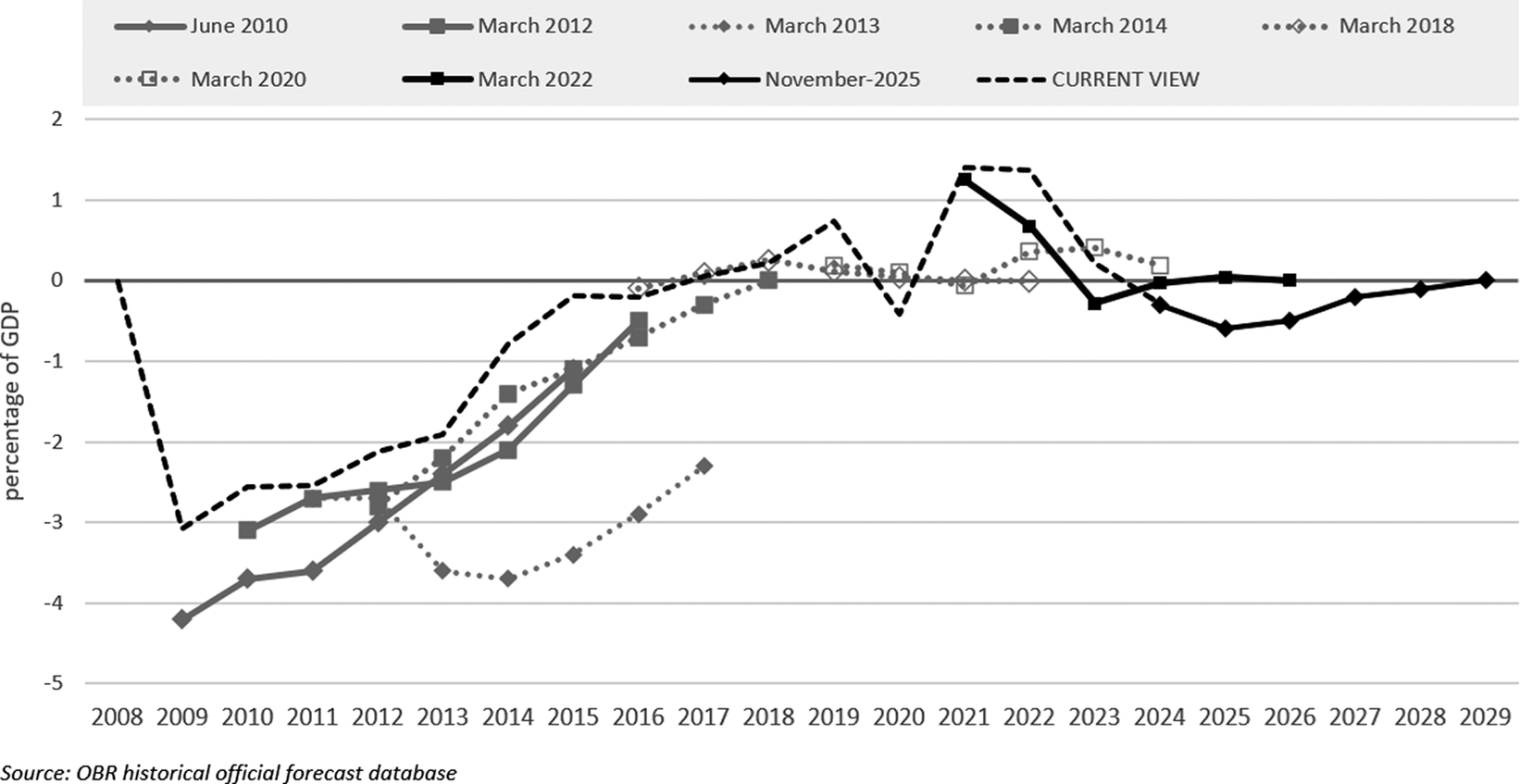
Figure 2 indicates the supply judgement is systemic in the United Kingdom (showing for clarity the position every few years), with the overall trajectory of the output gap little different now (indeed, narrower) to the original assessment in 2010—in spite of a substantial and widely recognised shortfall in GDP outcomes (quantified below). The main exception was the March 2013 assessment, discussed in Section 6 below.
OBR view of the output gap over time.

Figure 2. Long description
The x-axis represents years from 2008 to 2029. The y-axis represents the percentage of G D P, ranging from negative 5 to positive 2.
Legend items include various forecast dates from June 2010 to November 2025, plus a CURRENT VIE W.
Data trends:
* June 2010: Starts at negative 4.2 in 2009 and rises to negative 2.3 by 2017.
* March 2012: Starts at negative 3.1 in 2010 and rises to 0 by 2018.
* March 2013: Shows a dip to negative 3.7 in 2014 before rising.
* March 2020: Represented by open squares, hovering near 0 between 2021 and 2024.
* March 2022: Solid line with squares, peaking at positive 1.3 in 2021 before dropping to negative 0.3 in 2023.
* November 2025: Solid line with diamonds, showing a trough of negative 0.6 in 2025 and returning to 0 by 2029.
* CURRENT VIEW: A dashed black line showing a sharp drop to negative 3 in 2009, a recovery toward 0 by 2015, a peak of positive 1.4 in 2022, and a subsequent decline toward 0 by 2025.
Some are cautious about the output gap and potential output. Clift (Reference Clift2023, 35) cites Professor Sir Charles Bean regarding the latter as ‘“a very tricky concept”, that of “potential output—which is not there in the data, rather it’s the property of an economic model”’. He also cites Robert Chote: ‘you might have the economy weakening significantly and potential output weakening significantly at the same time. If so, the idea you can say anything terribly robust or meaningful about how the gap between the two has moved is for the birds’ (Clift, Reference Clift2023, 201). Clift (Reference Clift2023, 6) himself describes the output gap as ‘highly consequential but at the same time inherently elusive’. On this view, it is remarkable that the projection should be so little changed after such a long period when the economy has been under severe stress. And while the OBR claim to measure the output-gap indirectly with various proxies, the end result still conforms to the supply judgement. But only occasionally is any critique heard. Some exceptions are Adam and Cobhan (Reference Adam and Cobham2009) urging caution in the use of ‘real-time output gaps’, and Heimberger and Kapeller (Reference Heimberger and Kapeller2017) and Huber et al. (Reference Huber, Heimberger and Kapeller2017) drawing attention in particular to the pro-cyclicality of official estimates of potential.
The broadly unchanged output-gap trajectory reflects a judgement that the trend rate of GDP growth has fallen dramatically since the GFC, and relative to the earlier views of the OBR. TUC (2023) suggested GDP was around £400 billion lower in 2023 compared with a (simplistic) projection based on the trend rate of growth assumed by the OBR in 2010. Amounting to just under 20% of GDP, this gap might be set in the widespread shorthand that the UK economy has fallen short of pre-GFC trends by a third. If a role for demand is recognised, it should be possible to recapture at least some of this shortfall.
The projections take as given the OBR initial assessment of the trajectory for potential growth. And while this was relatively conservative, it might still have been too high given that growth ahead of the GFC was skewed towards the financial sector, and that one might expect economic growth to slow over time. Other more recent and ongoing shocks may have further undermined the supply-side: Brexit is likely in this category, and above all the climate crisis.
But there is a significant risk to the presumption that the whole shortfall belongs to the supply side. And while judgements as to potential output and the output gap have to be made as part of the forecasting process, the present analysis suggests a strong bias (Section 7). In practice, therefore, fiscal restraint is the permanent order of the day, when the imperative on a demand view is for expansionary policy (and this should include current spending). Without this spending, future growth falls even shorter, and the idea of a doom loop follows (TUC, 2023).
5. Public finances
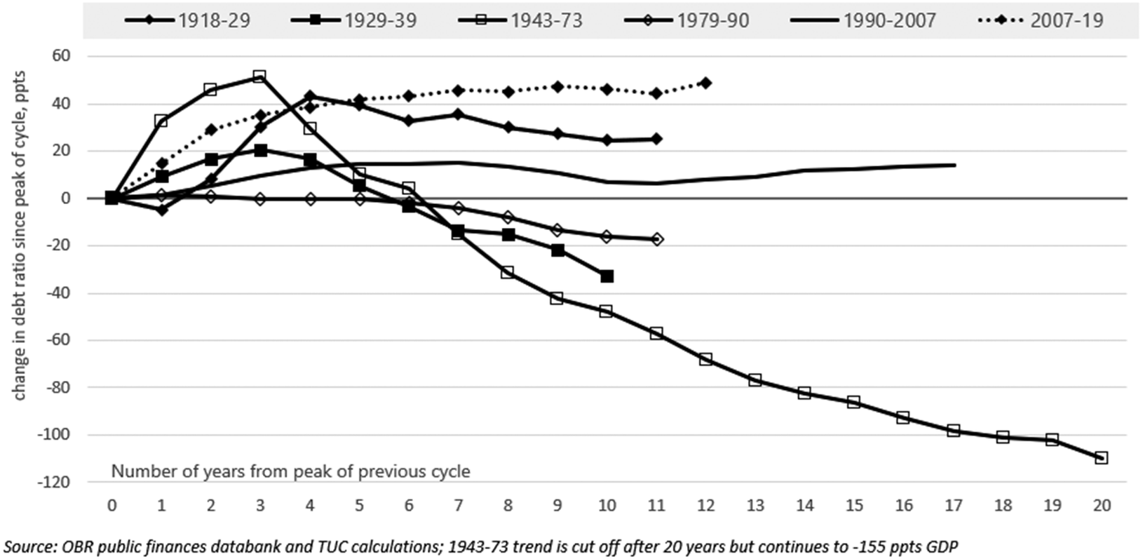
Whatever the objectives of the government, sustainability of the public finances is widely regarded as key. Figure 3 compares the trajectory of the public debt ratio over all UK economic cycles in the past 100 years (measured from peak to peak on GDP, with debt measured as change from the debt ratio at the GDP peak). The only even remotely close match to the present episode is the 1920s, which included the severe consolidation known as the ‘Geddes Axe’ (after Sir Eric Campbell Geddes, a British businessman and Conservative politician), a disastrous episode that was relevant context to Keynes seeking an alternative way forward. The chart shows how the two subsequent episodes (after the great depression and after the Second World War) were greatly more successful in terms of repairing the public finances (let alone economic growth). Indeed, fiscal policy in the great depression was expanded more vigorously than generally understood (Chick et al., Reference Chick, Pettifor and Tily2010).
Change in the public debt ratio over economic cycles from peak to peak.

Figure 3. Long description
A line graph with the x axis labeled Number of years from peak of previous cycle ranging from 0 to 20. The y axis is labeled change in debt ratio since start of recession, ppts, ranging from negative 120 to 60. All series begin at 0 on the x axis.
* 1918 to 29: Represented by a solid line with diamond markers. It peaks at year 4 around 40 ppts then declines steadily to negative 20 ppts by year 10.
* 1929 to 39: Represented by a solid line with square markers. It peaks at year 3 at 20 ppts then declines to negative 35 ppts by year 10.
* 1943 to 73: Represented by a solid line with open square markers. It rises sharply to 50 ppts at year 3 then enters a long, steep decline reaching negative 110 ppts by year 20.
* 1979 to 90: Represented by a solid line with open diamond markers. It remains near 0 until year 5 then declines gradually to negative 18 ppts by year 11.
* 1990 to 2007: Represented by a plain solid line. It rises slowly to 15 ppts by year 5 and remains relatively flat, ending at 15 ppts at year 17.
* 2007 to 19: Represented by a dotted line with diamond markers. It rises quickly to 45 ppts by year 8 and plateaus there through year 12.
A note at the bottom states the 1943 to 73 trend is cut off after 20 years but continues to negative 155 ppts GDP. Source is OBR public finances databank and TUC calculations.
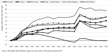
Nor was the 2010s outcome exclusive to the United Kingdom. The public finances have steadily deteriorated in all G7 economies except Germany (despite the country experiencing increasingly anaemic growth), and the deterioration predated the pandemic (Figure 4).Footnote 4
Change in the gross public debt ratio since 2007, G7 countries.

Figure 4. Long description
The horizontal X axis represents years from 2007 to 2025. The vertical Y axis represents the change in debt ratio since 2007 in percentage points, ranging from minus 10 to 90. All lines originate at 0 in 2007.
* Japan (dashed line) shows the highest increase, rising steadily to 60 points by 2014, peaking at 85 in 2020, and ending near 75 in 2025.
* United Kingdom (dotted line with diamonds) and United States (solid thick line) follow similar paths, rising to 40 points by 2012, spiking to approximately 65 in 2020, and stabilizing around 60 by 2025.
* France (solid line with squares) and Canada (solid line with circles) show a moderate increase, reaching 30 points by 2014, peaking at 50 in 2020, and ending between 35 and 50 in 2025.
* Italy (solid line with open squares) follows a similar trajectory to France but dips lower after 2020, ending near 35.
* Germany (solid line with open diamonds) shows the lowest change, peaking at 20 in 2012, declining to minus 5 in 2019, rising briefly to 5 in 2020, and returning to approximately 0 by 2025.
A universal sharp vertical spike is visible for all countries between 2019 and 2020. The source is cited as IMF global debt database.
International organisations have conceded this wider global failure, not least the IMF (2023) remark cited in the introduction. They elaborate:
The debt-reducing effects of fiscal adjustments are reinforced when accompanied by growth-enhancing structural reforms and strong institutional frameworks. At the same time, because these conditions and accompanying policies may not always be present, and partly because fiscal consolidation tends to slow GDP growth, consolidations on average have negligible effects on debt ratios. (IMF, 2023)
The point was made in the Jayadev and Konczal (Reference Jayadev and Konczal2010) critique of Alaesina and Arganda (Reference Alesina and Ardagna2009). And fundamentally, under weak growth, the (negative) demand effects will likely outweigh any (positive) structural effects. Pina et al. (Reference Pina, Hitschfeld and Miyahara2025) include a more extensive analysis of country experience (going back in one instance to 1978). But the authors draw a more problematic conclusion: ‘Sizeable fiscal consolidation, mainly on the expenditure side, has often taken place in the run-up to debt reduction episodes, with the debt-to-GDP ratio only starting to decline sometime after consolidation has begun’. As previously argued (Section 2), any turnaround was not thanks to the austerity policies in the first episode but followed the abandoning of austerity policies in the second episode.
Writing in the Financial Times, Victoria Chick and Ann Pettifor (Reference Chick and Pettifor2010) warned against setting up ‘false dichotomies: between cutters and postponers; between deficit-cutting and stimulus. The debate is not between these but between expenditure-cutting and stimulus’. Keynes saw that the impact of cuts on the public finances depends on the impact of cuts on the economy, writing ‘you will never balance the Budget through measures which reduce the national income’ (11 Jan. 1933, CW XXI, 149). Taking a lead from his analysis, Chick et al. (Reference Chick, Pettifor and Tily2010) looked at outcomes over relevant episodes: ‘The empirical evidence runs exactly counter to conventional thinking. Fiscal consolidations have not improved the public finances’ (ibid., p. 18). They judged: ‘when sustained, fiscal consolidation increases, not reduces, the public debt ratio and is in general associated with adverse economic conditions’ (ibid., p. 18). This was vindicated by subsequent UK outcomes. Moreover, the OECD analysis (Pina et al. (Reference Pina, Hitschfeld and Miyahara2025) and Table 1) indicates that for those countries where the debt position did improve, this followed when expansionary policies began.
Yet still the false dichotomy cannot be dislodged. The IMF and OECD concede challenges but cannot accept a different way forward. Keynes is still understood as ‘deficit spending’, a wholly inappropriate label for his position. In general, Keynes called for loan-financed public works (though ‘expenditures’ would have been better than ‘works’); as long as such expenditures generate a return that is higher than the cost of borrowing to finance them, then doing this will improve the public finances. The financial sector is key here. But the sector wrongly urged restraint at the start of austerity policies, and their continuing to do so is potentially standing in the way of improved public finances.
6. Monetary policy
The OBR does not operate in isolation: its forecast explicitly considers the approach of the Bank of England. As noted in OBR (2022), they assume ‘that the Monetary Policy Committee at the Bank of England sets monetary policy so that activity will return to its underlying potential level’. On their current assessment, the Bank judges the output gap for 2008 to 2021 to have been slightly more negative than the OBR, with the average difference at 0.9 ppts of GDP. The Bank has a higher output gap for 2022 (the year monetary policy was abruptly tightened) while their estimates for the output gap in 2023 and 2024 are similar to those of the OBR.
But the views of the two institutions have differed more significantly. In a retrospective of his time at the OBR, Robert Chote (Reference Chote2024) drew attention to the OBR forecasts in December 2012 and March 2013 ‘showing an extended period of spare capacity in the economy’ (see Figure 3); he continues:
…from which readers might have concluded that we felt the Bank needed more help from fiscal policy to bolster demand. That signal would have been clearer had we also forecast that inflation would persistently undershoot the target, but this would have had the Bank and Treasury straight on the phone.
Instead, they showed CPI dipping below target by only 0.1 ppts over 2013Q2 to 2014Q3. The OBR fully retreated by closing their output gap from the December 2013 forecast. But—critically—inflation did ‘persistently undershoot the target’ between 2014 and 2016.
On a longer view, up until the pandemic, inflation outcomes were at odds with the OBR assessment of the output gap (perhaps less so against the Bank view). While over 2010–2019 the output gap was meant to be closing, CPI inflation fell from 4.5% in 2011 to 0% in 2015; any rebound after Brexit was short lived, and disinflation had renewed before the pandemic hit (with CPI inflation at 1.4% in 2019Q4).
Yet monetary policy (including quantitative easing, QE) over this whole period was, at face value on a highly expansionary setting. Captured by the notion of monetary ease/fiscal restraint, the onus for expansionary policy was on the central bank. Moreover, repeated efforts to tighten policy failed: ‘Central banks have seen successive plans (in 2009, in 2013 and in 2018) to ‘normalise’ monetary policy frustrated by weak growth and low inflation’ (Turner, Reference Turner2021).
The sum of the parts is that monetary stimulus was deficient. Even despite near-zero interest rates and extensive QE programmes, monetary policy proved inadequate to close the output gap (as the OBR expected). The case that the output gap was significantly negative over this period is therefore reinforced.
Everything changed after the pandemic. With the global cost inflation that followed the end of lockdowns, central banks raised rates and halted or reversed QE processes. One result is seriously intensified pressures on fiscal policy, with interest rates on government debt moving alongside the rise in central bank rates. These have meant a steep rise in central government debt interest payments: in the United Kingdom from £38 billion a year in the five financial years ahead of the pandemic to around £100 billion a year over 2022–2023 to 2022–2025. ‘Fiscal headroom’ collapsed alongside these increased payments.
This very challenging environment was the context for the Labour government’s expansionary Budget in 2024. Given the Budget acted to raise demand, the OBR forecast a rise in interest rates (or rather that the forecast reduction would be smaller and slower). Their forecast for GDP 5 years out was virtually unchanged and living standards were also forecast to deteriorate relative to the March 2024 position under the previous government. At a Treasury Committee oral hearing Professor David Miles confirmed the OBR approach:
… ultimately the Bank of England’s role is to control inflation, which generally means bringing demand in the economy back in line with productive potential. For something that just boosts demand in the immediate short term, we take the view that the Bank of England will adjust to that, to bring the economy back to what you might call equilibrium, so that demand is in line with the supply potential of the economy. That would mean that the Keynesian demand effects—not trivial in the short run—tend to fade away if you look down the road.Footnote 5
To the extent that the OBR judgements around the output-gap are wrongheaded, the same is true of the Bank of England. Given the role of international commodity and energy markets, the renewed inflation does not affirm the institutional assessment. The case for the restrictive monetary policy is therefore not straightforward (TUC, 2025b, pp. 22–25). In the meantime the dominant effect is collapsed consumer demand, as well as the severe pressures on government finances. Moreover, there is the same danger of Bank of England policymakers mistaking weak aggregate demand for weak aggregate supply.
7. Modelling assumptions and fiscal frameworks
The above commentary has argued that the demand effects of fiscal policies might have been badly misjudged, and that any such misjudgement has repercussions continuing to the present. The ongoing risk is that modelling assumptions—especially crowding out—are operating to deny necessary expansionary policies. These modelling assumptions do not belong to OBR exclusively but are shared by the Bank of England and have been promoted by international organisations and supported by many academics. While policy is meant to be deliberative, there is a sense that these assumptions are setting the course rather than responding to outcomes. The above discussion might not prove the demand case, but at the very least the supply case is shown as unproven. Yet since 2010 policymakers have proceeded only on the supply view.
Clift (Reference Clift2023, 20) argues ‘there is always a politics of economic ideas, and economic orthodoxy is always a social construction’; therefore ‘The OBR … unavoidably takes positions within these inherently political debates through the assumptive foundations of its forecasting and the economic narratives it develops’ (ibid., 50). ‘Crowding out’ is one such ‘assumptive foundation’. Nonetheless, it should be open to evaluation. Based on the above, the assumption is seriously flawed. Indeed, outcomes over the 2010s might be regarded as a natural experiment that decisively refutes crowding out.
This is a significant conclusion. Moreover, if crowding out is flawed, then official estimates of the output gap have been and likely remain flawed. The public debt ratio has deteriorated as needed expansionary policy is denied. These conclusions stand regardless of the correct monetary policy response to the post-pandemic inflation.
Even while some debate has begun around potential shortcomings with OBR processes, an emerging danger is the lobbying for existing procedures to be strengthened. At the Lords Economic Affairs Committee, former OBR Chair Richard Hughes judged the UK public finances as particularly problematic, and suggested more rigid frameworks had enabled Southern European countries to turn the situation around.Footnote 6 I argued above that Southern European countries turned the situation around by changing policy. The danger is reading outcomes only based on the false dichotomy: public finances improved therefore austerity must have been done properly. The remarks further illustrate the difficulty of disengaging from the crowding-out mindset. Likewise the extent of consensus around the imperative to secure more ‘fiscal headroom’. All actions that withdraw demand are problematic if the output gap is negative.
Even those who have in recent years conceded the demand impact of austerity was underestimated (e.g. Editorial Board of the Financial Times, 2021) do not go on to address the implications for potential and the output gap, and so miss the possibility of repercussions into the present. The Report of the House of Lords Economic Affairs Committee (2026) does not address aggregate demand. The commentary above is suggestive of several issues that might be investigated more fully, not least country experience in more detail.
Blastland and Dilnot (Reference Blastland and Dilnot2023) call out groupthink:
Where there’s a consensus, it should be taken seriously; but a mainstream political consensus should not be mistaken for an economic one, and no apparent consensus should go without challenge … Nor should the BBC feel it can subcontract judgement about what’s reasonable or impartial to a few established names like the Bank of England, the OBR, the IFS or the Resolution Foundation, however respected.
In its submission for the Autumn Budget, TUC (2025b) called for ‘a new fiscal commission’. This was motivated in part by developments in other countries, and the wider idea of second-generation fiscal frameworks. Expenditure targets are regarded as of interest (Begg, Reference Begg2025, section 3.1), and a review of modelling was urged. The present essay has not examined the implications for either fiscal targets and rules or for wider institutional structures and arrangements. In terms of targets, it may be that expenditure targets rather than current deficit rules are compatible with the demand perspective. Likewise, as suggested throughout, a (non-rolling) target for a falling debt ratio should be compatible with the right model. Above all these are questions that belong after those related to modelling.
In an ideal world, these reviews would be a matter of routine, as part of existing processes between HMT, BoE and OBR. Ultimately, institutions might be strengthened and financial markets not disrupted. But the groupthink that is still manifest in public deliberations suggests an independent one-off review is needed before any material change might be fostered, and routine procedures devised and implemented. A relevant blueprint exists. In 1929 the Labour Government convened the Macmillan Inquiry after pressure from both trade unions and businesses (Konzelmann, Shipman and Tily, Reference Konzelmann, Shipman and Tilyforthcoming, final section). The Committee took on board the views of labour, business, finance, civil society, economists and other academics, and the Report (largely authored by Keynes) helped find a way forward from the great depression. A similar challenge is needed today.
Acknowledgements
The author thanks, without implication, an anonymous referee, the editors, and participants at the National Institute of Economic and Social Research workshop on ‘Fiscal Frameworks and Public Investment’ for useful comments. The views expressed in this article remain those of the author and should not be taken to represent those of the Trades Union Congress. Though I would still like to thank colleagues Nic Smith and Kate Bell for support and valuable advice. I also want to thank and honour Philip Turner (1950-2024) of the Bank for International Settlements and afterwards a visiting Fellow of NIESR who was for many years a generous friend to my work.