1 Introduction
Internal waves propagate beneath the fluid surface, with their largest vertical amplitudes occurring in the interior, and are a ubiquitous phenomenon in the ocean. One of the first observations of internal waves was reported by Helland-Hansen & Nansen (Reference Helland-Hansen and Nansen1909) more than a century ago, and they indicated that these kinds of ‘puzzling wave’ are irregular, and can appear randomly in the ocean. Oceanic internal solitary waves typically have much longer time scales and larger amplitudes than the analogous surface waves because of the much smaller density difference across the pycnocline than across the air–water interface. Here the pycnocline is the diffuse boundary between the upper lighter fluid and the lower heavier fluid. Internal solitary waves are commonly observed in the coastal zone, and, on a theoretical level, can be decomposed into an infinite set of vertical modes. Here the terminology ‘mode’ refers to the modal function describing the vertical structure. Mode 1 waves have the fastest phase speed and the simplest modal structure, typically a single maximum located at or near the pycnocline. Mode 2 waves are the next fastest, with a phase speed usually approximately one-third that of mode 1, and have a modal structure with two extrema. Note that the modal structure here refers to the vertical particle displacement, and, in general, the vertical structure for the density and velocity fields may be quite different. There are two different forms of mode 1 internal solitary waves, depression and elevation waves, with the isopycnal displaced downwards and upwards, respectively. For mode 2 waves, the corresponding wave shapes are called convex when the upper (lower) isopycnal is displaced upwards (downwards), and are called concave when the upper (lower) isopycnal is displaced downwards (upwards). Usually, observed mode 1 waves are depression waves when the near-surface isopycnal is displaced downwards.
Both mode 1 and mode 2 internal solitary waves have been observed. Liu et al. (Reference Liu, Chang, Hsu and Liang1998) identified and documented the dispersion and polarity change processes of the depression waves propagating shoreward from synthetic aperture radar (SAR) images, while Klymak & Moum (Reference Klymak and Moum2003) and Moum & Smyth (Reference Moum and Smyth2006) describe internal solitary waves of elevation from field observation. Both mode 1 and mode 2 waves were recorded by Farmer & Smith (Reference Farmer and Smith1980) in Knight Inlet, showing that mode 2 waves tended to occur in summer and mode 1 waves in winter. In contrast, Yang et al. (Reference Yang, Fang, Chang, Ramp, Kao and Tang2009) found mode 2 internal solitary waves more active in winter than in summer in the northern South China Sea, while mode 1 waves occurred in the opposite case. Mode 2 waves propagating with a mode 1 wave tail were documented by Farmer & Smith (Reference Farmer and Smith1980) and Shroyer, Moum & Nash (Reference Shroyer, Moum and Nash2010); and Akylas & Grimshaw (Reference Akylas and Grimshaw1992) gave a theoretical explanation for this phenomenon. Yang et al. (Reference Yang, Fang, Chang, Ramp, Kao and Tang2009) and Liu et al. (Reference Liu, Su, Hsu, Kuo and Ho2013) observed that mode 2 internal solitary waves appeared after mode 1 internal solitary waves, suggesting that the mode 2 waves were related to the mode 1 waves. A convex-type mode 2 internal solitary wave was found by Ramp et al. (Reference Ramp, Yang, Reeder and Bahr2012) on the northern Heng-Chun Ridge. There have been several laboratory studies of mode 2 solitary waves, and we mention the recent studies by Terletska et al. (Reference Terletska, Jung, Talipova, Maderich, Brovchenko and Grimshaw2016) and Deepwell et al. (Reference Deepwell, Stastna, Carr and Davies2017) of the interaction of a mode 2 solitary wave with a step and a narrow ridge, respectively. Mode 1 waves are much more common, and this may be because mode 2 waves do not propagate over such large distances as mode 1 waves (see Yang et al. Reference Yang, Tang, Chang, Liu, Hsu and Ramp2004, Reference Yang, Fang, Chang, Ramp, Kao and Tang2009, Reference Yang, Fang, Tang and Ramp2010; Shroyer et al. Reference Shroyer, Moum and Nash2010; Ramp et al. Reference Ramp, Yang, Reeder and Bahr2012). Helfrich & Melville (Reference Helfrich and Melville2006) provided an overview of internal solitary waves, while Lamb (Reference Lamb2014) reviewed the instabilities of internal waves.
Internal mode 1 waves are typically generated by barotropic tidal flow over topographic features (see Gerkema Reference Gerkema2001; Zhao & Alford Reference Zhao and Alford2006; Akylas et al. Reference Akylas, Grimshaw, Clarke and Tabaei2007; Grimshaw & Helfrich Reference Grimshaw and Helfrich2018), although a few other generation mechanisms have also been suggested. Akylas & Grimshaw (Reference Akylas and Grimshaw1992), Shroyer et al. (Reference Shroyer, Moum and Nash2010) and Yuan, Grimshaw & Johnson (Reference Yuan, Grimshaw and Johnson2018) show that a co-propagating mode 1 wave train can be generated by a mode 2 wave, with energy transfer from the higher mode to the lower mode. Although mode 1 waves have been extensively investigated, the less observed mode 2 waves have not received equivalent attention and research, and especially their generation mechanisms are not as well understood (see Yang et al. Reference Yang, Fang, Chang, Ramp, Kao and Tang2009). Nevertheless, some potential mechanisms for the generation of mode 2 waves have been proposed. An experimental and theoretical study by Helfrich & Melville (Reference Helfrich and Melville1986) found that the instability of a shoaling mode 1 wave may lead to the generation of a mode 2 wave. Vlasenko & Hutter (Reference Vlasenko and Hutter2001) found that a reflected and transmitted mode 2 wave may emerge when a mode 1 wave interacts with a localised sill. Mode 2 waves can also be produced at the head of gravity intrusions in laboratory studies (see Maxworthy Reference Maxworthy1980; Mehta, Sutherland & Kyba Reference Mehta, Sutherland and Kyba2002). Lamb & Warn-Varnas (Reference Lamb and Warn-Varnas2015) did detailed studies on shoaling internal solitary waves in the South China Sea under different background environments, with a mode 2 wave being generated at small-scale features in the bathymetry. Liang et al. (Reference Liang, Du, Li and He2018) found that mode 2 waves may arise when an initial mode 1 waves propagate into a horizontally varying stratification regime, and Liang & Li (Reference Liang and Li2019) indicated from field observations that a convex internal solitary wave may be generated by a shoaling semidiurnal mode 2 internal tide.
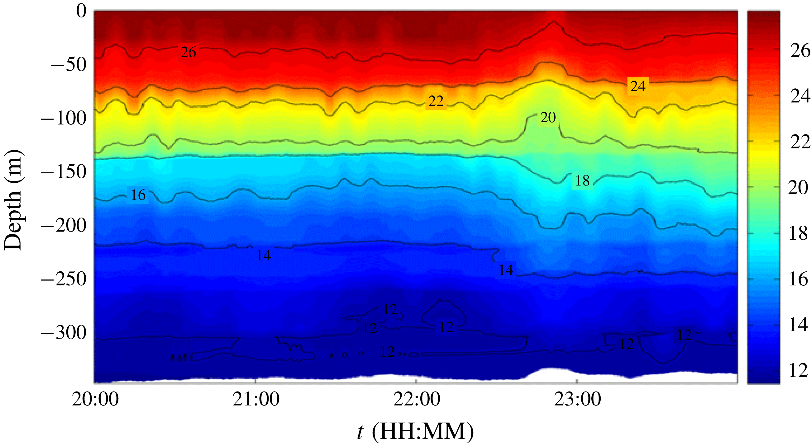
In this paper, we are concerned with the possible generation of a mode 2 wave as a mode 1 wave propagates shoreward from deep water, over the continental slope into shallow water. Figure 1 (from Liu et al. Reference Liu, Su, Hsu, Kuo and Ho2013) shows an observed mode 2 wave after the passing of a mode 1 solitary wave, which was probably generated on the continental shelf break near Dong-Sha Island. For this purpose we use the linear long-wave theory developed by Griffiths & Grimshaw (Reference Griffiths and Grimshaw2007) which describes the topographic coupling of a full set of linear long-wave modes. That theory was essentially developed to describe the generation of the internal tide by the flow of the barotropic tide over topography, but is adapted here to describe the generation of a mode 2 wave as a mode 1 wave propagates over variable depth. Once the mode 2 wave is formed, we use the Korteweg–de Vries (KdV) equation (2.1) to follow its evolution over the continental slope and shelf.
Temperature data (
 $^{\circ }\text{C}$
) showing a small mode 2 wave with an amplitude of 30 m at the mooring station on 24 May 2009 (reproduced with permission Liu et al.
Reference Liu, Su, Hsu, Kuo and Ho2013).

In § 2 we describe the theoretical formulation, the well-known KdV equation in § 2.1 and then in § 2.2 the linear long-wave theory, adapted from Griffiths & Grimshaw (Reference Griffiths and Grimshaw2007) to describe the generation of a mode 2 wave by a mode 1 wave propagating over topography, limited here to weak slopes. Then in § 3 we apply this theory to a three-layer fluid, for both a ‘thin’ and a ‘thick’ middle layer, with different topographic gradients. In § 4 we consider the application of the theory to a smooth density stratification with a diffuse pycnocline. Then in § 5 we consider two oceanic cases where mode 2 waves have been observed. We conclude in § 6.
2 Theoretical formulation
2.1 Korteweg–de Vries equation
For a single mode it is customary to invoke the KdV equation for the propagation of weakly nonlinear long internal waves over variable topography. In standard notation for a fluid of depth
 $h(x)$
, it is expressed as
 $$\begin{eqnarray}\displaystyle \frac{\unicode[STIX]{x2202}A}{\unicode[STIX]{x2202}t}+c\frac{\unicode[STIX]{x2202}A}{\unicode[STIX]{x2202}x}+\frac{1}{2Q}\frac{\unicode[STIX]{x2202}Q}{\unicode[STIX]{x2202}x}cA+\unicode[STIX]{x1D707}A\frac{\unicode[STIX]{x2202}A}{\unicode[STIX]{x2202}x}+\unicode[STIX]{x1D6FF}\frac{\unicode[STIX]{x2202}^{3}A}{\unicode[STIX]{x2202}x^{3}}=0; & & \displaystyle\end{eqnarray}$$
see Grimshaw (Reference Grimshaw1981) and the reviews by Helfrich & Melville (Reference Helfrich and Melville2006), Grimshaw (Reference Grimshaw2007) and Grimshaw et al. (Reference Grimshaw, Pelinovsky, Talipova and Kurkina2010). Here
 $\unicode[STIX]{x1D701}=A(x,t)\unicode[STIX]{x1D719}(z;h)$
is the leading-order expression for the vertical particle displacement. Using the Boussinesq approximation and in the absence of a background shear flow, the modal function
 $\unicode[STIX]{x1D719}(z;h)$
is determined by
 $$\begin{eqnarray}\displaystyle \frac{\unicode[STIX]{x2202}^{2}\unicode[STIX]{x1D719}}{\unicode[STIX]{x2202}z^{2}}+\frac{N^{2}}{c^{2}}\unicode[STIX]{x1D719}=0,\quad \unicode[STIX]{x1D719}=0,\quad z=0,-h(x),\quad N^{2}=-\frac{g}{\unicode[STIX]{x1D70C}_{0}}\frac{\unicode[STIX]{x2202}\unicode[STIX]{x1D70C}_{0}}{\unicode[STIX]{x2202}z}. & & \displaystyle\end{eqnarray}$$
Here
 $\unicode[STIX]{x1D70C}_{0}(z)$
is the background density field. This modal equation determines the modal function
 $\unicode[STIX]{x1D719}(z;h)$
and the linear long-wave speed
 $c(h)$
, where the
 $h$
dependence is parametric, since it is assumed that the depth
 $h(x)$
is slowly varying. The coefficients in (2.1) are given by
 $$\begin{eqnarray}\displaystyle & \displaystyle I\unicode[STIX]{x1D707}=3c^{2}\int _{-h}^{0}\unicode[STIX]{x1D70C}_{0}\left(\frac{\unicode[STIX]{x2202}\unicode[STIX]{x1D719}}{\unicode[STIX]{x2202}z}\right)^{3}\,\text{d}z, & \displaystyle\end{eqnarray}$$
 $$\begin{eqnarray}\displaystyle & \displaystyle I\unicode[STIX]{x1D6FF}=c^{2}\int _{-h}^{0}\unicode[STIX]{x1D70C}_{0}\unicode[STIX]{x1D719}^{2}\,\text{d}z, & \displaystyle\end{eqnarray}$$
 $$\begin{eqnarray}\displaystyle I=2c\int _{-h}^{0}\unicode[STIX]{x1D70C}_{0}\left(\frac{\unicode[STIX]{x2202}\unicode[STIX]{x1D719}}{\unicode[STIX]{x2202}z}\right)^{2}\text{d}z,\quad Q=c^{2}I. & & \displaystyle\end{eqnarray}$$
In general, the modal equation (2.2) determines an infinite set of modes. As discussed above, usually only mode 1,
 $\unicode[STIX]{x1D719}_{1}$
, with the fastest linear phase speed
 $c_{1}$
is considered. Then the KdV equation (2.1) describes the evolution of the amplitude of this mode. But importantly we note that the same KdV equation (2.1) can be used for a mode 2 wave, with coefficients determined by (2.3), (2.4) and (2.5) using the mode 2 modal function.
2.2 Linear long-wave theory
While the KdV equation (2.1) describes the long-time evolution of a single mode over variable topography, linear long-wave theory suffices as a first step to describe the generation of a mode 2 wave as a mode 1 wave moves over topography. Here we adapt the theory of Griffiths & Grimshaw (Reference Griffiths and Grimshaw2007), which used linear long-wave theory to decompose the wave field into a sum of vertical modes, noting that the full set of modal functions defined by (2.2) are complete. For our present purpose, we use a reduction of that theory restricted to just two modes, mode 1 and mode 2, in the expectation based on observations that any higher modes will have very small amplitudes. Note that in a three-layer fluid model, in the Boussinesq and rigid-lid approximation, this is formally exact. Then the wave field is given by
 $$\begin{eqnarray}\displaystyle \left.\begin{array}{@{}c@{}}\displaystyle \unicode[STIX]{x1D701}=\mathop{\sum }_{n=1}^{n=2}A_{n}(x,t)\unicode[STIX]{x1D719}_{n}(z;h),\\ \displaystyle u=\mathop{\sum }_{n=1}^{n=2}A_{n}(x,t)c_{n}(h)\frac{\unicode[STIX]{x2202}\unicode[STIX]{x1D719}_{n}(z;h)}{\unicode[STIX]{x2202}z},\\ \displaystyle p=\unicode[STIX]{x1D70C}_{0}\mathop{\sum }_{n=1}^{n=2}A_{n}(x,t)c_{n}^{2}(h)\frac{\unicode[STIX]{x2202}\unicode[STIX]{x1D719}_{n}(z;h)}{\unicode[STIX]{x2202}z}.\end{array}\right\} & & \displaystyle\end{eqnarray}$$
Here
 $\unicode[STIX]{x1D701}$
,
 $u$
and
 $p$
are the vertical particle displacement, the horizontal velocity and the dynamic pressure, respectively. The vertical velocity is
 $w=\unicode[STIX]{x2202}\unicode[STIX]{x1D701}/\unicode[STIX]{x2202}t$
and the density perturbation is
 $\unicode[STIX]{x1D70C}=N^{2}\unicode[STIX]{x1D701}/g$
. From Griffiths & Grimshaw (Reference Griffiths and Grimshaw2007) (see their equation (24)) the linear long-wave coupling between modes 1 and 2 with linear long-wave speeds
 $c_{1,2}$
is given by, for slowly varying
 $h(x)$
,
 $$\begin{eqnarray}\displaystyle & \displaystyle \frac{1}{c_{1}^{2}}\frac{\unicode[STIX]{x2202}^{2}U_{1}}{\unicode[STIX]{x2202}t^{2}}-\frac{\unicode[STIX]{x2202}^{2}U_{1}}{\unicode[STIX]{x2202}x^{2}}=-\unicode[STIX]{x1D6FE}\frac{\unicode[STIX]{x2202}h}{\unicode[STIX]{x2202}x}\frac{\unicode[STIX]{x2202}U_{2}}{\unicode[STIX]{x2202}x}, & \displaystyle\end{eqnarray}$$
 $$\begin{eqnarray}\displaystyle & \displaystyle \frac{1}{c_{2}^{2}}\frac{\unicode[STIX]{x2202}^{2}U_{2}}{\unicode[STIX]{x2202}t^{2}}-\frac{\unicode[STIX]{x2202}^{2}U_{2}}{\unicode[STIX]{x2202}x^{2}}=\unicode[STIX]{x1D6FE}\frac{\unicode[STIX]{x2202}h}{\unicode[STIX]{x2202}x}\frac{\unicode[STIX]{x2202}U_{1}}{\unicode[STIX]{x2202}x}, & \displaystyle\end{eqnarray}$$
 $$\begin{eqnarray}\displaystyle & \displaystyle \unicode[STIX]{x1D6FE}=\frac{2}{\unicode[STIX]{x1D706}_{1}-\unicode[STIX]{x1D706}_{2}}\left(\frac{\unicode[STIX]{x2202}\unicode[STIX]{x1D706}_{1}}{\unicode[STIX]{x2202}h}\frac{\unicode[STIX]{x2202}\unicode[STIX]{x1D706}_{2}}{\unicode[STIX]{x2202}h}\right)^{1/2}=\frac{4}{c_{2}^{2}-c_{1}^{2}}\left(c_{1}c_{2}\frac{\unicode[STIX]{x2202}c_{1}}{\unicode[STIX]{x2202}h}\frac{\unicode[STIX]{x2202}c_{2}}{\unicode[STIX]{x2202}h}\right)^{1/2},\quad \unicode[STIX]{x1D706}_{1}=\frac{1}{c_{1}^{2}},\quad \unicode[STIX]{x1D706}_{2}=\frac{1}{c_{2}^{2}}.\qquad & \displaystyle\end{eqnarray}$$
As noted above, this is a reduction from the full set in equation (24) of Griffiths & Grimshaw (Reference Griffiths and Grimshaw2007) by restriction to just two modes, and retention of only the leading-order topographic coupling terms when
 $h(x)$
is slowly varying; that is, terms such as
 $\unicode[STIX]{x2202}^{2}h/\unicode[STIX]{x2202}x^{2}$
or
 $(\unicode[STIX]{x2202}h/\unicode[STIX]{x2202}x)^{2}$
are omitted on the basis that the internal wave wavelengths we are considering here are much shorter than the topographic scale. The theory of Griffiths & Grimshaw (Reference Griffiths and Grimshaw2007) was developed for the horizontal velocity field in the form
 $u=U\unicode[STIX]{x2202}\unicode[STIX]{x1D713}(z;h)/\unicode[STIX]{x2202}z$
, whereas in the usual KdV theory described above by (2.6) the theory is developed for the vertical particle displacement
 $A\unicode[STIX]{x1D719}(z;h)$
, where the modal function
 $\unicode[STIX]{x1D713}\propto \unicode[STIX]{x1D719}$
. In the absence of a background shear flow, these are related by, temporarily omitting the modal index,
 $$\begin{eqnarray}\displaystyle u=U\frac{\unicode[STIX]{x2202}\unicode[STIX]{x1D713}}{\unicode[STIX]{x2202}z}=cA\frac{\unicode[STIX]{x2202}\unicode[STIX]{x1D719}}{\unicode[STIX]{x2202}z},\quad \unicode[STIX]{x1D713}(z)=K\unicode[STIX]{x1D719}(z),\quad K^{2}=\frac{1}{Ic}=\frac{c}{Q}. & & \displaystyle\end{eqnarray}$$
Hence we find that
 $$\begin{eqnarray}\displaystyle U=(cQ)^{1/2}A, & & \displaystyle\end{eqnarray}$$
where
 $Q$
and
 $I$
are the linear magnification and normalisation factors in the usual KdV theory, respectively (see (2.5)). Note that
 $Ic>0$
and
 $Qc>0$
from (2.5), so these expressions hold for both
 $c>0$
and
 $c<0$
.
The linear phase speeds
 $c_{1.2}$
are obtained from the modal equation (2.2) for the modal function
 $\unicode[STIX]{x1D719}_{r}(z;h)$
, here indexed with the mode number,
 $$\begin{eqnarray}\displaystyle \frac{\unicode[STIX]{x2202}^{2}\unicode[STIX]{x1D719}_{r}}{\unicode[STIX]{x2202}z^{2}}+\unicode[STIX]{x1D706}_{r}N^{2}\unicode[STIX]{x1D719}_{r}=0,\quad \unicode[STIX]{x1D719}_{r}=0,\quad z=0,-h,\quad r=1,2. & & \displaystyle\end{eqnarray}$$
These satisfy the orthogonality conditions:
 $$\begin{eqnarray}\displaystyle \left.\begin{array}{@{}c@{}}\displaystyle \int _{-h}^{0}\unicode[STIX]{x1D70C}_{0}\frac{\unicode[STIX]{x2202}\unicode[STIX]{x1D719}_{1}}{\unicode[STIX]{x2202}z}\frac{\unicode[STIX]{x2202}\unicode[STIX]{x1D719}_{2}}{\unicode[STIX]{x2202}z}\,\text{d}z=0,\\ \displaystyle \int _{-h}^{0}\unicode[STIX]{x1D70C}_{0}\left(\frac{\unicode[STIX]{x2202}\unicode[STIX]{x1D719}_{1}}{\unicode[STIX]{x2202}z}\right)^{2}\text{d}z=I_{1},\quad \int _{-h}^{0}\unicode[STIX]{x1D70C}_{0}\left(\frac{\unicode[STIX]{x2202}\unicode[STIX]{x1D719}_{2}}{\unicode[STIX]{x2202}z}\right)^{2}\text{d}z=I_{2}.\end{array}\right\} & & \displaystyle\end{eqnarray}$$
In (2.9),
 $\unicode[STIX]{x2202}\unicode[STIX]{x1D706}_{1}/\unicode[STIX]{x2202}h$
,
 $\unicode[STIX]{x2202}\unicode[STIX]{x1D706}_{2}/\unicode[STIX]{x2202}h$
,
 $\unicode[STIX]{x2202}c_{1}/\unicode[STIX]{x2202}h$
and
 $\unicode[STIX]{x2202}c_{2}/\unicode[STIX]{x2202}h$
denote derivatives with respect to
 $h$
. Formally they can be found by differentiating (2.12) with respect to
 $h$
, so that
 $$\begin{eqnarray}\displaystyle \frac{\unicode[STIX]{x2202}^{2}\hat{\unicode[STIX]{x1D719}}_{r}}{\unicode[STIX]{x2202}z^{2}}+\unicode[STIX]{x1D706}_{r}N^{2}\hat{\unicode[STIX]{x1D719}}_{r}=-\frac{\unicode[STIX]{x2202}\unicode[STIX]{x1D706}_{r}}{\unicode[STIX]{x2202}h}N^{2}\unicode[STIX]{x1D719}_{r},\quad \hat{\unicode[STIX]{x1D719}}_{r}=0,\quad z=0,\quad \hat{\unicode[STIX]{x1D719}}_{r}=\frac{\unicode[STIX]{x2202}\unicode[STIX]{x1D719}_{r}}{\unicode[STIX]{x2202}z},\quad z=-h,\quad & & \displaystyle\end{eqnarray}$$
where
 $\hat{\unicode[STIX]{x1D719}}_{r}$
denotes the derivative of
 $\unicode[STIX]{x1D719}_{r}$
with respect to
 $h$
. Equation (2.14) is an inhomogeneous version of the modal equation, and a regular solution requires a compatibility condition,
 $$\begin{eqnarray}\displaystyle \frac{\unicode[STIX]{x2202}\unicode[STIX]{x1D706}_{r}}{\unicode[STIX]{x2202}h}\int _{-h}^{0}\left(\frac{\unicode[STIX]{x2202}\unicode[STIX]{x1D719}_{r}}{\unicode[STIX]{x2202}z}\right)^{2}\text{d}z=-\left(\frac{\unicode[STIX]{x2202}\unicode[STIX]{x1D719}_{r}}{\unicode[STIX]{x2202}z}\right)^{2}(z=-h). & & \displaystyle\end{eqnarray}$$
Thus
 $\unicode[STIX]{x2202}\unicode[STIX]{x1D706}_{r}/\unicode[STIX]{x2202}h$
and hence
 $\unicode[STIX]{x2202}c_{r}/\unicode[STIX]{x2202}h$
can be found directly from the modal function, without any need for explicit differentiation with respect to
 $h$
. Note especially that
 $\unicode[STIX]{x2202}\unicode[STIX]{x1D706}_{r}/\unicode[STIX]{x2202}h<0$
and so
 $\unicode[STIX]{x1D706}_{r}$
increases as
 $h$
decreases, that is,
 $c_{r}$
decreases as
 $h$
decreases, which holds for all density stratification and depth profiles. Thus the coupling coefficient
 $\unicode[STIX]{x1D6FE}$
in (2.9) is always well defined (since
 $\unicode[STIX]{x1D706}_{1}<\unicode[STIX]{x1D706}_{2}$
) and
 $\unicode[STIX]{x1D6FE}<0$
. These expressions hold for general slowly varying
 $h(x)$
but we shall now suppose henceforth that there is the usual oceanic situation that
 $h\rightarrow h_{a,b}$
as
 $x\rightarrow \pm \infty$
with
 $h_{b}>h_{a}$
. Specifically, we will suppose that
 $h=h_{b}$
for
 $x<0$
, and
 $h=h_{a}$
for
 $x>L>0$
.
Since we are assuming that
 $h(x)$
is slowly varying, for each mode we use the change of variables,
 $$\begin{eqnarray}\displaystyle T=\int _{0}^{x}\frac{\text{d}x}{c},\quad X=T-t, & & \displaystyle\end{eqnarray}$$
 $$\begin{eqnarray}\displaystyle \left.\begin{array}{@{}c@{}}\displaystyle \frac{\unicode[STIX]{x2202}^{2}U}{\unicode[STIX]{x2202}t^{2}}=\frac{\unicode[STIX]{x2202}^{2}U}{\unicode[STIX]{x2202}X^{2}},\quad \frac{\unicode[STIX]{x2202}U}{\unicode[STIX]{x2202}x}=\frac{1}{c}\left(\frac{\unicode[STIX]{x2202}U}{\unicode[STIX]{x2202}X}+\frac{\unicode[STIX]{x2202}U}{\unicode[STIX]{x2202}T}\right),\\ \displaystyle \frac{\unicode[STIX]{x2202}^{2}U}{\unicode[STIX]{x2202}x^{2}}=\frac{1}{c^{2}}\left(\frac{\unicode[STIX]{x2202}^{2}U}{\unicode[STIX]{x2202}X^{2}}+2\frac{\unicode[STIX]{x2202}^{2}U}{\unicode[STIX]{x2202}X\unicode[STIX]{x2202}T}+\frac{\unicode[STIX]{x2202}^{2}U}{\unicode[STIX]{x2202}T^{2}}\right)-\frac{1}{c^{3}}\frac{\unicode[STIX]{x2202}c}{\unicode[STIX]{x2202}T}\left(\frac{\unicode[STIX]{x2202}U}{\unicode[STIX]{x2202}X}+\frac{\unicode[STIX]{x2202}U}{\unicode[STIX]{x2202}T}\right).\end{array}\right\} & & \displaystyle\end{eqnarray}$$
Hence in each modal equation, the operator
 $$\begin{eqnarray}\displaystyle \frac{1}{c^{2}}\frac{\unicode[STIX]{x2202}^{2}U}{\unicode[STIX]{x2202}t^{2}}-\frac{\unicode[STIX]{x2202}^{2}U}{\unicode[STIX]{x2202}x^{2}}=-\frac{2}{c^{2}}\frac{\unicode[STIX]{x2202}^{2}U}{\unicode[STIX]{x2202}X\unicode[STIX]{x2202}T}-\frac{1}{c^{2}}\frac{\unicode[STIX]{x2202}^{2}U}{\unicode[STIX]{x2202}T^{2}}+\frac{1}{c^{3}}\frac{\unicode[STIX]{x2202}c}{\unicode[STIX]{x2202}T}\left(\frac{\unicode[STIX]{x2202}U}{\unicode[STIX]{x2202}X}+\frac{\unicode[STIX]{x2202}U}{\unicode[STIX]{x2202}T}\right). & & \displaystyle\end{eqnarray}$$
Using the transformation (2.11) and neglecting the slowly varying second and third terms on the right-hand side,
 $$\begin{eqnarray}\displaystyle \frac{1}{c^{2}}\frac{\unicode[STIX]{x2202}^{2}U}{\unicode[STIX]{x2202}t^{2}}-\frac{\unicode[STIX]{x2202}^{2}U}{\unicode[STIX]{x2202}x^{2}}\sim -\frac{2}{c^{3/2}}\frac{\unicode[STIX]{x2202}^{2}B}{\unicode[STIX]{x2202}X\unicode[STIX]{x2202}T},\quad B=Q^{1/2}A,\quad U=c^{1/2}B. & & \displaystyle\end{eqnarray}$$
This is for a right-going wave. A left-going wave is found by replacing
 $t$
with
 $-t$
in the definition of
 $X$
in (2.16).
Hence the coupled system (2.7) and (2.8) can be expressed as
 $$\begin{eqnarray}\displaystyle & \displaystyle \frac{\unicode[STIX]{x2202}^{2}B_{1}}{\unicode[STIX]{x2202}X_{1}\unicode[STIX]{x2202}T_{1}}=\frac{\unicode[STIX]{x1D6FE}c_{1}^{1/2}c_{2}^{1/2}}{2}\frac{\unicode[STIX]{x2202}h}{\unicode[STIX]{x2202}T_{1}}\frac{\unicode[STIX]{x2202}B_{2}}{\unicode[STIX]{x2202}X_{1}}, & \displaystyle\end{eqnarray}$$
 $$\begin{eqnarray}\displaystyle & \displaystyle \frac{\unicode[STIX]{x2202}^{2}B_{2}}{\unicode[STIX]{x2202}X_{2}\unicode[STIX]{x2202}T_{2}}=-\frac{\unicode[STIX]{x1D6FE}c_{1}^{1/2}c_{2}^{1/2}}{2}\frac{\unicode[STIX]{x2202}h}{\unicode[STIX]{x2202}T_{2}}\frac{\unicode[STIX]{x2202}B_{1}}{\unicode[STIX]{x2202}X_{2}}. & \displaystyle\end{eqnarray}$$
Here
 $(X_{i},T_{i}),~i=1,2$
, are the pair
 $(X,T)$
in (2.16) with
 $c$
replaced with
 $c_{i}$
, respectively. Note that, although the pairs
 $(X_{1},T_{1})$
and
 $(X_{2},T_{2})$
are different, they are not independent; see the discussion below. In the absence of any coupling terms, equations (2.20) and (2.21) yield the linear adiabatic law that
 $B_{1}=B_{1}(X_{1})$
and
 $B_{2}=B_{2}(X_{2})$
, where
 $X_{i}$
is the phase
 $X$
in (2.16). More generally we can add a KdV extension for each mode, that is,
 $$\begin{eqnarray}\displaystyle \frac{\unicode[STIX]{x2202}B}{\unicode[STIX]{x2202}T}\rightarrow \frac{\unicode[STIX]{x2202}B}{\unicode[STIX]{x2202}T}+\unicode[STIX]{x1D708}B\frac{\unicode[STIX]{x2202}B}{\unicode[STIX]{x2202}X}+\unicode[STIX]{x1D706}\frac{\unicode[STIX]{x2202}^{3}B}{\unicode[STIX]{x2202}X^{3}},\quad \unicode[STIX]{x1D708}=\frac{\unicode[STIX]{x1D707}}{cQ^{1/2}}\quad \unicode[STIX]{x1D706}=\frac{\unicode[STIX]{x1D6FF}}{c^{3}}, & & \displaystyle\end{eqnarray}$$
after applying the transformations (2.16) to the KdV equation (2.1), and
 $\unicode[STIX]{x1D707}$
and
 $\unicode[STIX]{x1D6FF}$
are defined by (2.3) and (2.4).
As noted above, the pair
 $X,T$
are different for the two modes, that is,
 $$\begin{eqnarray}\displaystyle T_{1}=\int _{0}^{x}\frac{\text{d}x}{c_{1}},\quad X_{1}=T_{1}-t,\quad T_{2}=\int _{0}^{x}\frac{\text{d}x}{c_{2}},\quad X_{2}=T_{2}-t. & & \displaystyle\end{eqnarray}$$
However, there are only two independent variables,
 $(x,t)$
, and hence these pairs are related. In particular,
 $T_{1}=T_{1}(x)$
and
 $T_{2}=T_{2}(x)$
are each functions of
 $x$
alone, and hence are related as follows:
 $$\begin{eqnarray}\displaystyle T_{2}(T_{1})=\int _{0}^{T_{1}}\frac{c_{1}(T_{1}^{\prime })}{c_{2}(T_{1}^{\prime })}\,\text{d}T_{1}^{\prime },\quad \text{and}\quad T_{1}(T_{2})=\int _{0}^{T_{2}}\frac{c_{2}(T_{2}^{\prime })}{c_{1}(T_{2}^{\prime })}\,\text{d}T_{2}^{\prime }. & & \displaystyle\end{eqnarray}$$
Note that the origin for
 $T_{1}$
and
 $T_{2}$
is placed at
 $x=0$
, so that in the deep water
 $x<0$
before the slope
 $T_{1}<0$
and
 $T_{2}<0$
. Further we can write
 $$\begin{eqnarray}\displaystyle X_{2}=X_{2}(T_{1},t)=T_{2}(T_{1})-t,\quad X_{1}=X_{1}(T_{2},t)=T_{1}(T_{2})-t, & & \displaystyle\end{eqnarray}$$
expressing
 $X_{2,1}$
in terms of
 $T_{1,2}$
and
 $t$
. Then on eliminating
 $t$
, we can express
 $X_{2}$
as a function of
 $X_{1}$
and
 $T_{1}$
and likewise
 $X_{1}$
as a function of
 $X_{2}$
and
 $T_{2}$
:
 $$\begin{eqnarray}\displaystyle X_{2}=X_{1}+T_{2}(T_{1})-T_{1},\quad X_{1}=X_{2}+T_{1}(T_{2})-T_{2}. & & \displaystyle\end{eqnarray}$$
In the sequel it is useful to note that in the deep water
 $x<0$
before the shelf, these expressions take a particularly simple form, since in
 $x<0$
,
 $c_{2}/c_{1}=R<1$
is a constant. Then from (2.24), (2.25) and (2.26), in
 $x<0$
,
 $$\begin{eqnarray}\displaystyle x<0,\quad T_{1}(T_{2})=RT_{2}<0,\quad T_{2}(T_{1})=\frac{T_{1}}{R}<0, & & \displaystyle\end{eqnarray}$$
 $$\begin{eqnarray}\displaystyle x<0,\quad X_{1}=RT_{2}-t=X_{2}+(R-1)T_{2},\quad \quad X_{2}=\frac{T_{1}}{R}-t=X_{1}+\left(\frac{1}{R}-1\right)T_{1}. & & \displaystyle \nonumber\\ \displaystyle & & \displaystyle\end{eqnarray}$$
Similar simple forms hold on the shelf
 $x>L$
, where again the ratio
 $c_{2}/c_{1}$
is a constant.
2.3 Generation of a mode 2 wave
In the presence of coupling, we can only apply the transformation (2.16) to one of the two modes. Here, noting that the coupling terms are small, proportional to
 $\unicode[STIX]{x2202}h/\unicode[STIX]{x2202}x=(1/c_{1})(\unicode[STIX]{x2202}h/\unicode[STIX]{x2202}T_{1})$
, we consider the case of a mode 1 wave, possibly obeying a KdV equation (2.22), and generating a small mode 2 wave over the slope. In this situation, the coupling term representing the back effect of mode 2 on mode 1 can be ignored, and we assume that the mode 1 wave satisfies the KdV equation (2.22) evaluated with mode 1 coefficients,
 $$\begin{eqnarray}\displaystyle \frac{\unicode[STIX]{x2202}B_{1}}{\unicode[STIX]{x2202}T_{1}}+\unicode[STIX]{x1D708}_{1}B_{1}\frac{\unicode[STIX]{x2202}B_{1}}{\unicode[STIX]{x2202}X_{1}}+\unicode[STIX]{x1D706}_{1}\frac{\unicode[STIX]{x2202}^{3}B_{1}}{\unicode[STIX]{x2202}X_{1}^{3}}=0. & & \displaystyle\end{eqnarray}$$
Then using the transformation (2.16), the mode 2 equation (2.8) becomes a forced equation, which when expressed in the coordinates
 $(X_{1},T_{1})$
becomes
 $$\begin{eqnarray}\displaystyle \left\{\frac{c_{1}^{2}-c_{2}^{2}}{c_{1}^{2}c_{2}^{2}}\right\}\frac{\unicode[STIX]{x2202}^{2}B_{2}}{\unicode[STIX]{x2202}X_{1}^{2}}\sim \left\{\frac{c_{1}}{c_{2}}\right\}^{1/2}\frac{\unicode[STIX]{x1D6FE}}{c_{1}^{2}}\frac{\unicode[STIX]{x2202}h}{\unicode[STIX]{x2202}T_{1}}\frac{\unicode[STIX]{x2202}B_{1}}{\unicode[STIX]{x2202}X_{1}}, & & \displaystyle\end{eqnarray}$$
 $$\begin{eqnarray}\displaystyle \frac{\unicode[STIX]{x2202}^{2}B_{2}}{\unicode[STIX]{x2202}X_{1}^{2}}\sim \tilde{\unicode[STIX]{x1D6FE}}\frac{\unicode[STIX]{x2202}h}{\unicode[STIX]{x2202}T_{1}}\frac{\unicode[STIX]{x2202}B_{1}}{\unicode[STIX]{x2202}X_{1}},\quad \tilde{\unicode[STIX]{x1D6FE}}=\left\{\frac{c_{1}}{c_{2}}\right\}^{1/2}\frac{c_{2}^{2}}{c_{1}^{2}-c_{2}^{2}}\unicode[STIX]{x1D6FE}. & & \displaystyle\end{eqnarray}$$
A particular solution is
 $$\begin{eqnarray}\displaystyle B_{2p}(X_{1},T_{1})=-\tilde{\unicode[STIX]{x1D6FE}}\frac{\unicode[STIX]{x2202}h}{\unicode[STIX]{x2202}T_{1}}\int _{X_{1}}^{\infty }B_{1}(X_{1}^{\prime },T_{1})\,\text{d}X_{1}^{\prime }. & & \displaystyle\end{eqnarray}$$
Here we have imposed the boundary condition that there are no waves ahead of the forcing
 $B_{1}$
wave, that is,
 $B_{2p}\rightarrow 0$
as
 $X_{1}\rightarrow \infty$
;
 $B_{2p}$
has a phase
 $X_{1}$
, the same as
 $B_{1}$
, and hence is slaved to mode 1, and propagates with the same speed as the forcing wave
 $B_{1}$
, that is,
 $c_{1}$
to leading order in the forcing wave amplitude. Note that, since here
 $\tilde{\unicode[STIX]{x1D6FE}}<0$
and
 $\unicode[STIX]{x2202}h/\unicode[STIX]{x2202}T_{1}<0$
,
 $B_{2p}$
will have the opposite orientation to
 $B_{1}$
, that is, it will be a wave of elevation or depression, according as
 $B_{1}$
is a wave of depression or elevation. Further, if
 $B_{1}$
is localised with respect to the phase
 $X_{1}$
, then
 $B_{2p}$
has the structure of a shelf which extends to
 $X_{1}\rightarrow -\infty$
for each fixed
 $T_{1}$
. However, because of the factor
 $\unicode[STIX]{x2202}h/\unicode[STIX]{x2202}T_{1}$
in
 $B_{2p}$
(2.32), this particular solution can only be non-zero in the region where
 $\unicode[STIX]{x2202}h/\unicode[STIX]{x2202}T_{1}\neq 0$
, that is, the slope region
 $0<T_{1}<L$
, say. This implies that this slaved wave cannot propagate past
 $T_{1}=L$
, and once the forcing wave
 $B_{1}$
has passed into the shallow water
 $T_{1}>L$
, this slaved wave becomes stationary, and depends only on
 $T_{1}$
. This stationary form can be found by letting
 $X_{1}\rightarrow -\infty$
in (2.32) to give
 $$\begin{eqnarray}\displaystyle B_{2p}^{stat}(T_{1})=-\tilde{\unicode[STIX]{x1D6FE}}\frac{\unicode[STIX]{x2202}h}{\unicode[STIX]{x2202}T_{1}}{\mathcal{M}}_{1},\quad {\mathcal{M}}_{1}=\int _{-\infty }^{\infty }B_{1}(X_{1}^{\prime },T_{1})\,\text{d}X_{1}^{\prime }, & & \displaystyle\end{eqnarray}$$
where
 ${\mathcal{M}}_{1}$
is the ‘mass’ of the forcing
 $B_{1}$
wave.
To this particular solution we can add any free solution of the homogeneous solution for mode 2, which has a phase
 $X_{2}$
(that is,
 $X$
in (2.16) with
 $c=c_{2}$
). To leading order this is just
 $B_{2f}=F(X_{2})$
, where
 $F(\cdot )$
is an arbitrary function, and depends on
 $X_{2}$
only. Hence the complete general solution for
 $B_{2}$
for right-going waves is
 $$\begin{eqnarray}\displaystyle B_{2}(X_{1},T_{1})=B_{2p}(X_{1},T_{1})+F(X_{2})=-\tilde{\unicode[STIX]{x1D6FE}}\frac{\unicode[STIX]{x2202}h}{\unicode[STIX]{x2202}T_{1}}\int _{X_{1}}^{\infty }B_{1}(X_{1}^{\prime },T_{1})\,\text{d}X_{1}^{\prime }+F(X_{2}), & & \displaystyle\end{eqnarray}$$
where we note that
 $X_{2}$
can be expressed in terms of
 $X_{1}$
and
 $T_{1}$
through (2.26). To determine the functional form of
 $F(\cdot )$
, we recall that
 $\unicode[STIX]{x2202}h/\unicode[STIX]{x2202}T_{1}\neq 0$
only over the slope region and in particular
 $\unicode[STIX]{x2202}h/\unicode[STIX]{x2202}T_{1}=0$
for
 $T_{1}<0$
(
 $x<0$
). We suppose that initially there is only a mode 1 wave in the deep water
 $T_{1}<0$
(
 $x<0$
), and so we can impose the initial condition that for
 $t\leqslant 0$
the mode 1 wave is in the deep water and there is no mode 2 wave,
 $B_{2}=0$
. From (2.23), at
 $t=0$
,
 $X_{2}=T_{2}=\int _{0}^{x}\text{d}x/c_{2}$
and
 $X_{1}=T_{1}=\int _{0}^{x}\text{d}x/c_{1}$
, where we recall that
 $T_{1}$
and
 $T_{2}$
are functionally related through (2.24). We can now determine
 $F(X_{2})$
as
 $t\rightarrow 0$
from
 $$\begin{eqnarray}\displaystyle F(T_{2})=\tilde{\unicode[STIX]{x1D6FE}}\frac{\unicode[STIX]{x2202}h}{\unicode[STIX]{x2202}T_{1}}\int _{T_{1}}^{\infty }B_{1}(T_{1},X_{1}^{\prime })\,\text{d}X_{1}^{\prime },\quad \text{where }T_{1}=T_{1}(T_{2}), & & \displaystyle\end{eqnarray}$$
from (2.24). Thus the free solution is given by replacing
 $T_{2}$
in (2.35) by
 $X_{2}$
,
 $$\begin{eqnarray}\displaystyle B_{2f}(X_{2})=F(X_{2})=\tilde{\unicode[STIX]{x1D6FE}}\frac{\unicode[STIX]{x2202}h}{\unicode[STIX]{x2202}T_{1}}\int _{T_{1}}^{\infty }B_{1}(T_{1},X_{1}^{\prime })\,\text{d}X_{1}^{\prime },\quad \text{where now }T_{1}=T_{1}(X_{2}). & & \displaystyle\end{eqnarray}$$
The full solution (2.34) is the sum of
 $B_{2p}$
(2.32) and
 $B_{2f}$
(2.36).
This free mode 2 wave (2.36) is the main item of interest. If
 $B_{1}$
is localised and so
 $B_{2p}$
has the structure of a shelf, then
 $B_{2f}$
inherits some aspects of this shelf structure, and under KdV dynamics this shelf will develop into an undular bore. Importantly, however, because of the prefactor
 $\unicode[STIX]{x2202}h/\unicode[STIX]{x2202}T_{1},T_{1}=T_{1}(X_{2})$
,
 $B_{2f}$
is a localised function of
 $X_{2}$
, defined only over the range
 $0<T_{1}(X_{2})<L$
, and propagates with a speed
 $c_{2}$
(in
 $x{-}t$
space) without change of form. In particular, it will continue to propagate beyond
 $x>L$
after the particular solution has become stationary with the form (2.33).
Note that (2.26) can be used to express
 $X_{2}$
in terms of
 $X_{1}$
and
 $T_{1}$
, and so we can express
 $B_{2f}$
as a function of
 $X_{1}$
and
 $T_{1}$
. This is needed for plotting
 $B_{2p},B_{2f}$
and the sum
 $B_{2}$
as functions of
 $X_{1}=T_{1}-t$
for several fixed values of
 $T_{1}$
(that is, a time series at several fixed locations), or as functions of
 $T_{1}$
for fixed values of
 $t$
. Importantly, for the free wave component
 $B_{2f}$
,
 $X_{2}=X_{2}(X_{1},T_{1})$
from (2.26) and varies over the whole range
 $-\infty <X_{2}<\infty$
. Thus in the functional relationship
 $T_{1}(X_{2})$
in (2.36) where
 $X_{2}$
has replaced
 $T_{2}$
in
 $T_{1}(T_{2})$
(2.24), the full range of
 $-\infty <T_{2}<\infty$
is needed. In particular, we recall from (2.27) that, in the range
 $-\infty <T_{2}<0$
,
 $T_{1}=RT_{2}$
and so
 $$\begin{eqnarray}\displaystyle -\infty <X_{2}<0,\quad T_{1}(X_{2})=RX_{2}=RT_{1}-t=RX_{1}+(1-R)T_{1}. & & \displaystyle\end{eqnarray}$$
From (2.36),
 $B_{2f}=0$
for
 $T_{1}(X_{2})<0$
, which using (2.37) is the regime
 $RT_{1}<t$
, where we recall that
 $R=c_{2}/c_{1}$
in the deep water,
 $T_{1}<0$
.
For instance, suppose that
 $B_{1}$
is a KdV solitary wave asymptotic solution of (2.29),
 $$\begin{eqnarray}\displaystyle B_{1}=a\,\text{sech}^{2}(K(X_{1}-P(T_{1}))),\quad \frac{\unicode[STIX]{x2202}P}{\unicode[STIX]{x2202}T_{1}}=V=\frac{\unicode[STIX]{x1D708}_{1}a}{3}=4\unicode[STIX]{x1D706}_{1}K^{2},\quad a=a_{0}\unicode[STIX]{x1D70E}^{1/3},\qquad & & \displaystyle\end{eqnarray}$$
where
 $\unicode[STIX]{x1D70E}=|\unicode[STIX]{x1D708}_{1}|/\unicode[STIX]{x1D706}_{1}$
normalised so that
 $\unicode[STIX]{x1D70E}=1$
in the deep water before the slope. We set
 $P=0$
at
 $T_{1}=0$
so that the solitary wave enters the slope at
 $x=0$
when
 $t=0$
. Then the particular solution (2.32) becomes
 $$\begin{eqnarray}\displaystyle B_{2p}(X_{1},T_{1})=-\tilde{\unicode[STIX]{x1D6FE}}\frac{\unicode[STIX]{x2202}h}{\unicode[STIX]{x2202}T_{1}}\frac{a}{K}\{1-\tanh (K(X_{1}-P(T_{1})))\}, & & \displaystyle\end{eqnarray}$$
where we remind the reader that all the coefficients and parameters in (2.39) are functions of
 $T_{1}$
. In particular,
 ${\mathcal{M}}_{1}=2a/K$
(2.33). The free solution (2.36) becomes
 $$\begin{eqnarray}\displaystyle B_{2f}(X_{2})=\tilde{\unicode[STIX]{x1D6FE}}\frac{\unicode[STIX]{x2202}h}{\unicode[STIX]{x2202}T_{1}}\frac{a}{K}\{1-\tanh (K(T_{1}-P(T_{1})))\}. & & \displaystyle\end{eqnarray}$$
Here, on the right-hand side, we use (2.24) to find
 $T_{1}(T_{2})$
and then replace
 $T_{2}$
with
 $X_{2}$
.
In general, we will need to use interpolation to obtain the expressions (2.24) and hence the key functional relationship
 $T_{1}(X_{2})$
where
 $X_{2}$
has replaced
 $T_{2}$
. However, a useful guide to the outcome is obtained by using the approximation that the ratio
 $c_{2}/c_{1}=R$
is a constant, not only on
 $x<0$
, but also on
 $x>0$
. Indeed, it transpires that, in the applications we examine, this is quite a good approximation. Then from (2.27) and (2.28) we obtain the explicit analytical form
 $T_{1}(X_{2})=RX_{2}=RX_{1}+(1-R)T_{1}=T_{1}-Rt$
, showing as expected that this free wave propagates with speed
 $Rc_{1}=c_{2}$
in
 $x{-}t$
space.
3 Application: three-layer fluid model
There have been several theoretical studies of mode 2 internal solitary waves using a three-layer fluid model. Yang et al. (Reference Yang, Fang, Tang and Ramp2010) examined the characteristics of mode 2 internal solitary wave types in an ideal three-layer fluid system, using the KdV solitary wave solutions. They found that the middle layer thickness played a key role in determining whether the waves were of convex or concave type, and used this analysis to interpret some observations of mode 2 waves in the northern South China Sea. The study by Yuan et al. (Reference Yuan, Grimshaw and Johnson2018) shows the evolution of mode 2 internal solitary waves over a slope-shelf topography in a three-layer fluid model, based on a variable-coefficient KdV equation and also simulations using the MITgcm (Massachusetts Institute of Technology general circulation model), a three-dimensional primitive equation model, with fully nonlinear, non-hydrostatic terms (see Marshall et al. Reference Marshall, Adcroft, Hill, Perelman and Heisey1997a ,Reference Marshall, Hill, Perelman and Adcroft b ). Here we consider a three-layer fluid model, as described by Yuan et al. (Reference Yuan, Grimshaw and Johnson2018) for a different purpose, adapted here for the interaction of a mode 1 solitary wave with topography resulting in the generation of a mode 2 wave. Note that the MITgcm simulation uses a smoothed three-layer stratification and not the discrete three-layer fluid model described here.
The background density field is given by
 $$\begin{eqnarray}\displaystyle \unicode[STIX]{x1D70C}_{0}(z) & = & \displaystyle (\unicode[STIX]{x1D70C}_{2}+\unicode[STIX]{x0394}\unicode[STIX]{x1D70C}){\mathcal{H}}(-z-h_{1}-h_{2})\nonumber\\ \displaystyle & & \displaystyle +\,\unicode[STIX]{x1D70C}_{2}{\mathcal{H}}(-z-h_{1}){\mathcal{H}}(z+h_{1}+h_{2})+(\unicode[STIX]{x1D70C}_{2}-\unicode[STIX]{x0394}\unicode[STIX]{x1D70C}){\mathcal{H}}(z+h_{1}),\end{eqnarray}$$
where
 $h_{1}$
,
 $h_{2}$
and
 $h_{3}$
are the thickness of the three layers from top to bottom, respectively,
 $h=h_{1}+h_{2}+h_{3}$
. Note that the pycnocline depths
 $h_{1}$
and
 $h_{2}$
are fixed in this three-layer fluid model, but
 $h_{3}$
varies, because the total depth
 $h=h(x)=h_{1}+h_{2}+h_{3}(x)$
varies over the slope. Density
 $\unicode[STIX]{x1D70C}_{2}$
is that of the middle layer and
 $\unicode[STIX]{x0394}\unicode[STIX]{x1D70C}$
is the density difference across each interface; and
 ${\mathcal{H}}(\cdot )$
is the Heaviside function. Since
 $N^{2}=0$
in each layer, the modal function is given by, from (2.2),
 $$\begin{eqnarray}\displaystyle \left.\begin{array}{@{}c@{}}\displaystyle \unicode[STIX]{x1D719}=-C_{1}\frac{z}{h_{1}},\quad -h_{1}\leqslant z\leqslant 0,\\ \displaystyle \unicode[STIX]{x1D719}=C_{1}\frac{z+h_{1}+h_{2}}{h_{2}}-C_{2}\frac{z+h_{1}}{h_{2}},\quad -h_{1}-h_{2}<z<-h_{1},\\ \displaystyle \unicode[STIX]{x1D719}=C_{2}\frac{z+h}{h_{3}},\quad -h\leqslant z\leqslant -h_{1}-h_{2}.\end{array}\right\} & & \displaystyle\end{eqnarray}$$
Note that
 $\unicode[STIX]{x1D719}=C_{1}$
at the upper interface
 $z=-h_{1}$
, and
 $\unicode[STIX]{x1D719}=C_{2}$
at the lower interface
 $z=-h_{1}-h_{2}$
. The continuity of pressure across each interface is ensured by the jump conditions
 $c^{2}[\unicode[STIX]{x1D719}_{z}]_{-}^{+}+g^{\prime }\unicode[STIX]{x1D719}=0$
,
 $g^{\prime }=g\unicode[STIX]{x0394}\unicode[STIX]{x1D70C}/\unicode[STIX]{x1D70C}_{2}$
,
 $$\begin{eqnarray}\displaystyle \left.\begin{array}{@{}c@{}}\displaystyle c^{2}\left\{C_{1}\left(\frac{1}{h_{1}}+\frac{1}{h_{2}}\right)-\frac{C_{2}}{h_{2}}\right\}-g^{\prime }C_{1}=0,\\ \displaystyle c^{2}\left\{C_{2}\left(\frac{1}{h_{2}}+\frac{1}{h_{3}}\right)-\frac{C_{1}}{h_{2}}\right\}-g^{\prime }C_{2}=0,\end{array}\right\} & & \displaystyle\end{eqnarray}$$
 $$\begin{eqnarray}\displaystyle 2g^{\prime }\unicode[STIX]{x1D706}=\frac{2g^{\prime }}{c^{2}}=\left(\frac{1}{h_{1}}+\frac{2}{h_{2}}+\frac{1}{h_{3}}\right)\mp \left\{\left(\frac{1}{h_{1}}-\frac{1}{h_{3}}\right)^{2}+\frac{4}{h_{2}^{2}}\right\}^{1/2}. & & \displaystyle\end{eqnarray}$$
The signs
 $\mp$
correspond to mode 1 and mode 2, respectively, so that, as required,
 $c_{1}>c_{2}$
. It then follows that
 $$\begin{eqnarray}\displaystyle \frac{C_{1}}{C_{2}}=R=H\pm (H^{2}+1)^{1/2},\quad \frac{C_{2}}{C_{1}}=\frac{1}{R}=-H\pm (H^{2}+1)^{1/2},\quad H=\frac{h_{2}}{2}\left(\frac{1}{h_{3}}-\frac{1}{h_{1}}\right). & & \displaystyle \nonumber\\ \displaystyle & & \displaystyle\end{eqnarray}$$
The solution is normalised by
 $\max [|\unicode[STIX]{x1D719}|]=1$
, so that
 $\max [|C_{1}|,|C_{2}|]=1$
. For mode 1,
 $C_{1,2}>0$
and either the maximum of
 $|\unicode[STIX]{x1D719}(z)|$
occurs at the upper interface if
 $H>0,~h_{1}>h_{3}$
and
 $1=C_{1}>C_{2}>0$
, or at the lower interface if
 $H<0,~h_{1}<h_{3}$
and
 $1=C_{2}>C_{1}$
. For mode 2,
 $C_{1}C_{2}<0$
and the maximum of
 $|\unicode[STIX]{x1D719}(z)|$
occurs at the lower interface if
 $H>0$
and
 $1=C_{2}>0>C_{1}>-1$
, or at the upper interface if
 $H<0$
and
 $1=C_{1}>0>C_{2}>-1$
. Thus if a mode 2 wave is a wave of elevation, then this corresponds to a convex wave if the maximum of
 $|\unicode[STIX]{x1D719}(z)|$
occurs at the upper interface,
 $H<0,~h_{1}<h_{3}$
, but corresponds to a concave wave if the maximum of
 $|\unicode[STIX]{x1D719}(z)|$
occurs at the lower interface,
 $H>0,~h_{1}>h_{3}$
. This description is reversed if it is a wave of depression, which then corresponds to a concave wave if the maximum of
 $|\unicode[STIX]{x1D719}(z)|$
occurs at the upper interface,
 $H<0,~h_{1}<h_{3}$
, but corresponds to a convex wave if the maximum of
 $|\unicode[STIX]{x1D719}(z)|$
occurs at the lower interface,
 $H>0,~h_{1}>h_{3}$
. Note that from (3.4)
 $$\begin{eqnarray}\displaystyle 2g^{\prime }\frac{\unicode[STIX]{x2202}\unicode[STIX]{x1D706}}{\unicode[STIX]{x2202}h}=\frac{1}{h_{3}^{2}}\left\{-1\pm \frac{H}{(H^{2}+1)^{1/2}}\right\}. & & \displaystyle\end{eqnarray}$$
As required,
 $\unicode[STIX]{x2202}\unicode[STIX]{x1D706}/\unicode[STIX]{x2202}h<0$
for both modes. Also, in our main case of interest when
 $h_{1}<h_{3}$
, so that
 $H<0$
,
 $\unicode[STIX]{x2202}\unicode[STIX]{x1D706}_{1}/\unicode[STIX]{x2202}h<\unicode[STIX]{x2202}\unicode[STIX]{x1D706}_{2}/\unicode[STIX]{x2202}h<0$
. From (2.9)
 $$\begin{eqnarray}\displaystyle \unicode[STIX]{x1D6FE}=-\frac{h_{2}}{2h_{3}^{2}(H^{2}+1)}. & & \displaystyle\end{eqnarray}$$
For fixed
 $h_{1},h_{3}$
,
 $|\unicode[STIX]{x1D6FE}|\rightarrow 0$
as
 $h_{2}\rightarrow 0$
, that is, the coupling of the modes becomes smaller as the middle layer becomes thinner.
The KdV coefficients
 $\unicode[STIX]{x1D707}$
and
 $\unicode[STIX]{x1D6FF}$
in (2.22) are given by
 $$\begin{eqnarray}\displaystyle & \displaystyle I\unicode[STIX]{x1D707}=3c^{2}\left\{-\frac{C_{1}^{3}}{h_{1}^{2}}+\frac{C_{2}^{3}}{h_{3}^{2}}+\frac{(C_{1}-C_{2})^{3}}{h_{2}^{2}}\right\}, & \displaystyle\end{eqnarray}$$
 $$\begin{eqnarray}\displaystyle & \displaystyle I\unicode[STIX]{x1D6FF}=c_{1}^{2}\left\{C_{1}^{2}\frac{h_{1}+h_{2}}{3}+C_{2}^{2}\frac{h_{3}+h_{2}}{3}+C_{1}C_{2}\frac{h_{2}}{3}\right\}, & \displaystyle\end{eqnarray}$$
 $$\begin{eqnarray}\displaystyle & \displaystyle I=2c\left\{\frac{C_{1}^{2}}{h_{1}}+\frac{C_{2}^{2}}{h_{3}}+\frac{(C_{1}-C_{2})^{2}}{h_{2}}\right\}. & \displaystyle\end{eqnarray}$$
It is well known that if
 $\unicode[STIX]{x1D707}_{1}>0~({<}0)$
then mode 1 solitary waves are waves of elevation (depression). However, if
 $\unicode[STIX]{x1D707}_{2}>0~({<}0)$
, implying that mode 2 solitary waves are waves of elevation (depression), then this corresponds to a convex or a concave wave depending on the location of the maximum of
 $|\unicode[STIX]{x1D719}|$
as described above.
We have now obtained explicit expressions for all the coefficients and parameters in the mode 2 slaved wave (2.39) and the mode 2 free wave (2.40), and so proceed with two examples.
3.1 Illustrative examples
Now, given a suitable expression for the depth profile
 $h(x)$
, and a choice for layer depths
 $h_{1}$
and
 $h_{2}$
, we can proceed to plot these as a function of
 $x$
at a set of increasing times
 $t$
. We set
 $$\begin{eqnarray}\displaystyle h(x)=425-75\tanh (1\times 10^{-4}x), & & \displaystyle\end{eqnarray}$$
which represents a smooth transition from deep water depth of 500 m to a shallow water depth 350 m. Note that the origin of
 $x$
is at mid-slope here rather than at the bottom of the slope as in the theoretical development in § 2. Hence all expressions there should have a corresponding translation of the
 $x$
origin. The layer depths are set at
 $h_{1}=120~\text{m}$
and we will show two cases for
 $h_{2}=40~\text{m}$
and
 $h_{2}=80~\text{m}$
. For these settings,
 $h_{3}$
varies from 340 m, 300 m in the deep water to 190 m, 150 m in the shallow water, and in both cases
 $h_{1}<h_{3}$
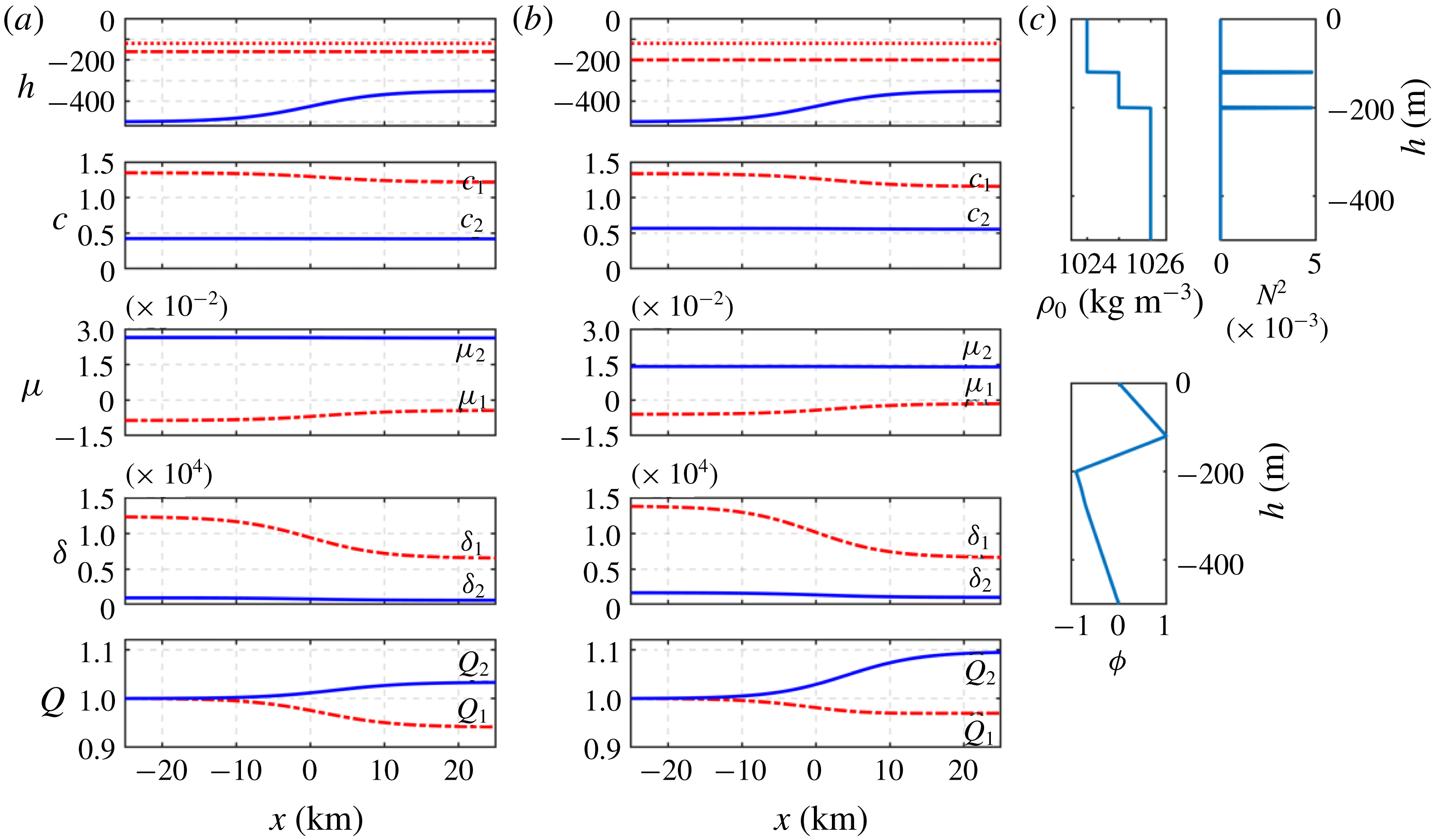
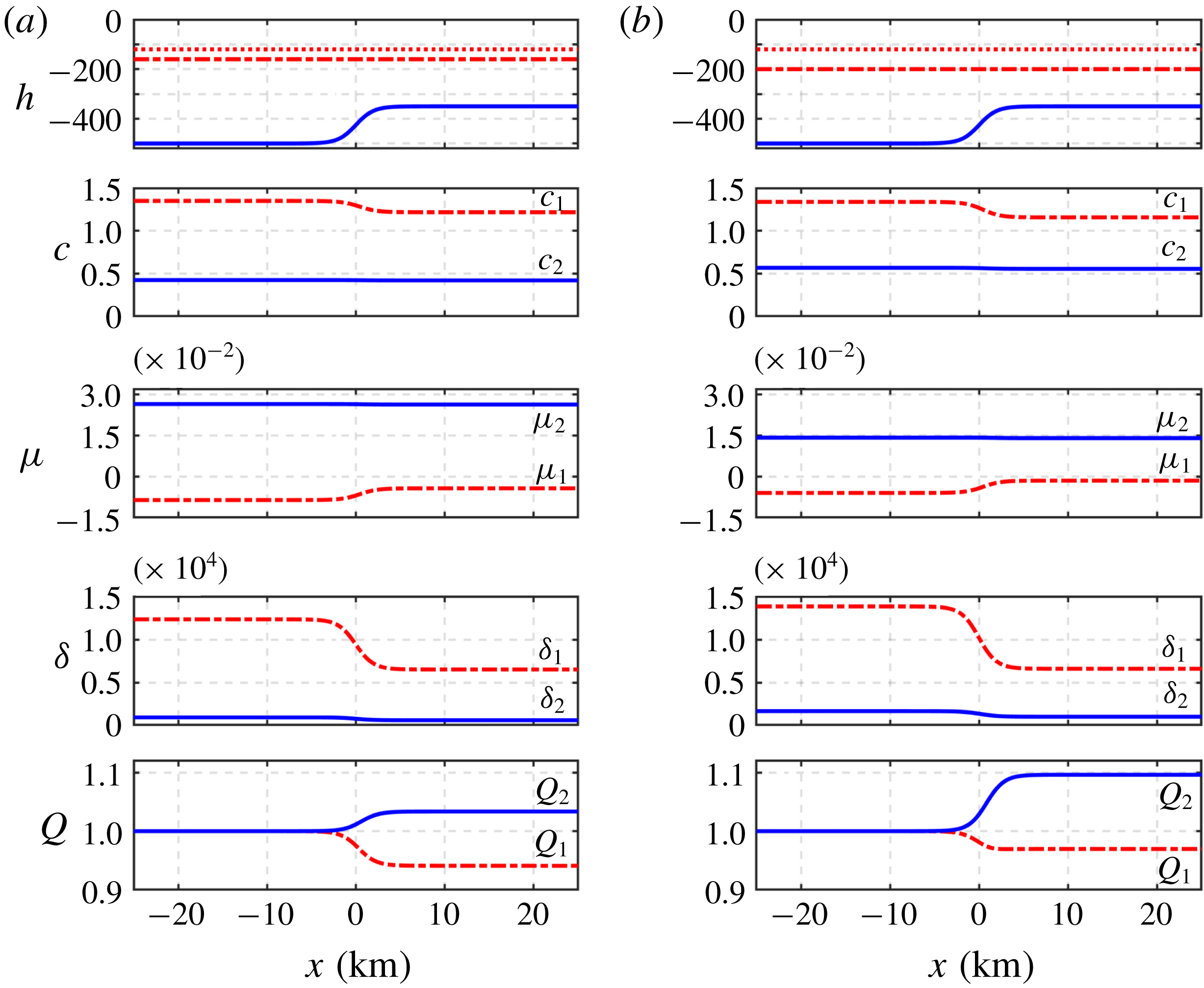
throughout, so that the pycnocline remains ‘near-surface’ throughout. The set-up is shown in figure 2. For the mode 1 solitary wave (2.38), the coefficients
 $\unicode[STIX]{x1D707}_{1},~\unicode[STIX]{x1D6FF}_{1}$
and
 $Q_{1}$
can now be calculated from (3.8), (3.9), (3.10) and (2.5) and are also shown in figure 2. Hence we can find the transformed coefficients
 $\unicode[STIX]{x1D708}_{1}$
and
 $\unicode[STIX]{x1D706}_{1}$
in (2.22). Coefficients for mode 2 waves can also be obtained similarly. We set the initial solitary wave amplitude in (2.38) as
 $a_{0}=-5$
m, noting that for the present parameter settings
 $\unicode[STIX]{x1D707}_{1}<0$
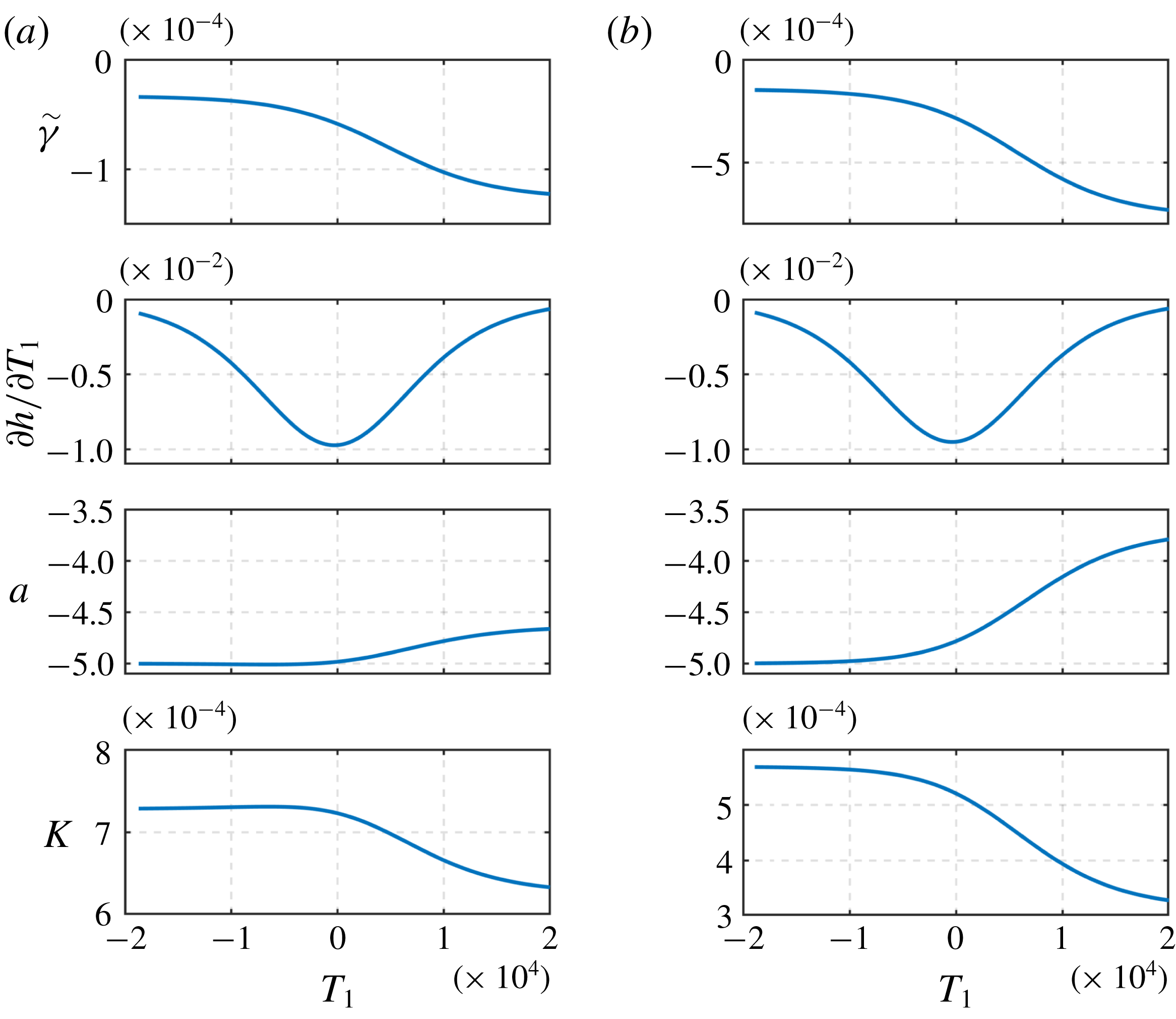
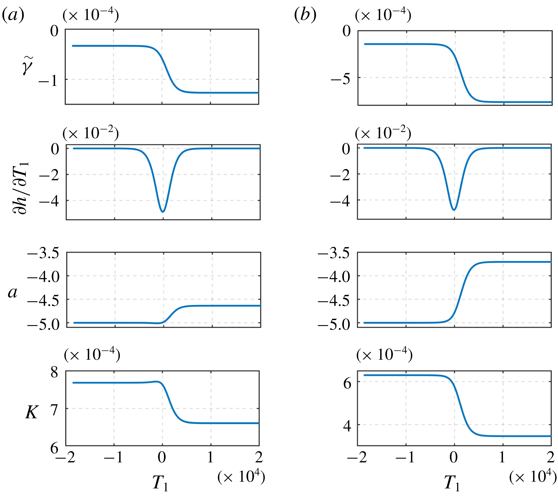
over the whole slope and so there is no polarity change. In figure 3 we show the expressions
 $\tilde{\unicode[STIX]{x1D6FE}}$
and
 $\unicode[STIX]{x2202}h/\unicode[STIX]{x2202}T_{1}$
and the solitary wave parameters
 $a$
and
 $K$
as functions of
 $T_{1}$
.
(c) The stratification at the start point of the slope-shelf region in the three-layer fluid model. Top: density profile and buoyancy frequency, represented by
 $N^{2}$
(
 $\text{s}^{-2}$
); bottom: modal function for mode 2. (a,b) The set-up of the three-layer fluid model with depth given by (3.11) and the coefficients of the KdV equation (2.1) for mode 1 and mode 2 waves. The middle layer thickness is 40 m in (a), and 80 m in (b). From top to bottom the panels show the layer depths (dotted and dash-dotted red lines) and total depth (solid blue lines), the phase speeds
 $c_{1,2}$
in units m s
 $^{-1}$
, and the nonlinear coefficients
 $\unicode[STIX]{x1D707}_{1,2}$
(2.3), the dispersive coefficients
 $\unicode[STIX]{x1D6FF}_{1,2}$
(2.4) and the linear magnification factor
 $Q_{1,2}$
(2.5) in units of
 $\text{s}^{-1},~\text{m}^{3}~\text{s}^{-1}$
and
 $1$
, respectively.

Parameters of the particular (2.39) and free (2.40) solutions in the three-layer fluid set-up (3.11) with different middle layer thicknesses: (a)
 $h_{2}=40~\text{m}$
and (b)
 $h_{2}=80~\text{m}$
. The expressions
 $\tilde{\unicode[STIX]{x1D6FE}}$
and
 $\unicode[STIX]{x2202}h/\unicode[STIX]{x2202}T_{1}$
are in units
 $\text{m}^{-1}$
and
 $\text{m}~\text{s}^{-1}$
, respectively, and the parameters
 $a$
and
 $K$
of the mode 1 solitary wave (2.38) are in units m and m
 $^{-1}$
, respectively.


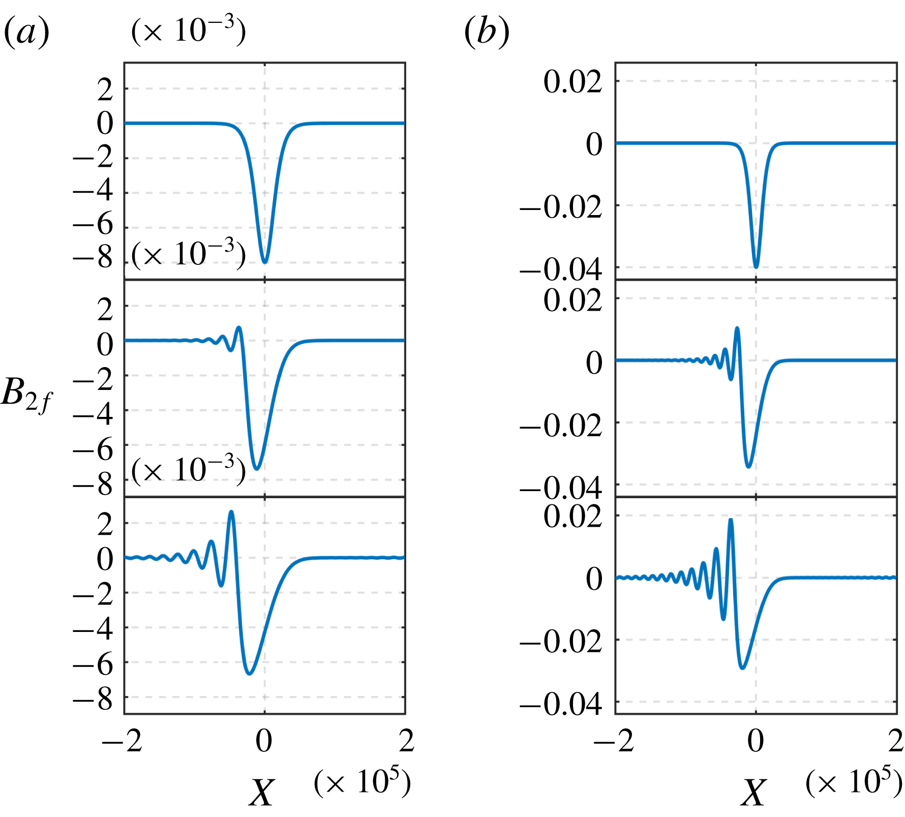
Plots of the evolution of the free mode 2 wave under KdV dynamics (3.12) with the initial condition (3.13). From top to bottom, the distances from the initial point are 0 km, 25 km and 50 km, respectively. The depth is given by (3.11) and (a,b) correspond to middle layer thickness of 40 m and 80 m, respectively.

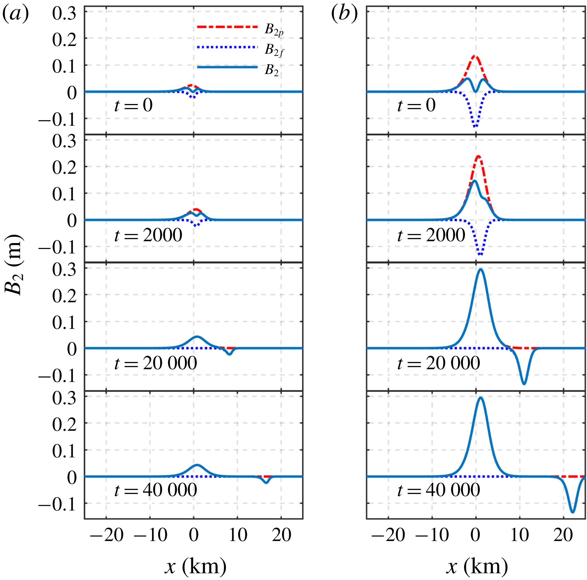
Figure 4 shows the evolution of the slaved wave (2.39) and the free wave (2.40). As expected, initially the free mode 2 wave and the slaved mode 2 wave are formed with the same amplitude and shape. The slaved wave then propagates with speed
 $c_{1}$
and increases in amplitude until the forcing mode 1 wave reaches the shallow water, when it is arrested and reaches its final steady state (2.33). In contrast, the free wave propagates with speed
 $c_{2}$
unchanged in form and eventually passes the forced wave and enters the shallow water. Note that with the present parameters, the slaved wave is one of elevation, while the free wave is one of depression. The most striking feature of these simulations is that the amplitudes are four times larger for the ‘thick’ pycnocline case (
 $h_{2}=80~\text{m}$
) than in the ‘thin’ pycnocline case (
 $h_{2}=40~\text{m}$
). This can be directly attributed to the four-fold increase in
 $\tilde{\unicode[STIX]{x1D6FE}}$
(figure 3), which in turn is due mainly to the difference in
 $\unicode[STIX]{x2202}c_{2}/\unicode[STIX]{x2202}h$
, although the change in
 $c_{2}$
with
 $h$
is hardly perceptible from the plot.
In general, the final amplitude of the slaved wave is determined from the maximum value of the product
 $-2\tilde{\unicode[STIX]{x1D6FE}}(\unicode[STIX]{x2202}h/\unicode[STIX]{x2202}T_{1})a/K$
, which depends only on
 $x$
. In the ‘thick’ pycnocline case the peak amplitude is approximately 0.06 m, which is
 $1.2\,\%$
of the forcing wave amplitude. In contrast, the free wave amplitude, which does not change with time, is determined from (2.40) by its value at
 $t=0$
, when
 $X_{2}=T_{2}$
and
 $T_{1}=T_{1}(T_{2})$
. Assuming that
 $KL\gg 1$
(in these simulations
 $KL$
is of the order of
 $10$
), this can be estimated approximately from the minimum value of the product
 $\tilde{\unicode[STIX]{x1D6FE}}(\unicode[STIX]{x2202}h/\unicode[STIX]{x2202}T_{1})a/K$
over a restricted range where
 $KT_{1}$
is of the order of unity. In the ‘thick’ pycnocline case the free wave amplitude is approximately
 $-0.03~\text{m}$
, approximately one-half the amplitude of the slaved wave and
 $0.6\,\%$
of the forcing wave amplitude. In terms of ocean applications, these may seem to be rather small, and possibly unobservable, but we remark that this is a linear theory, and the complete solution scales with the magnitude of the forcing amplitude
 $a_{0}/K_{0}$
, that is, with
 $a_{0}^{1/2}$
: a four-fold increase in
 $a_{0}$
to
 $-20~\text{m}$
would increase the response by a factor of
 $2$
. More pertinently, the percentage estimates remain in place when the forcing amplitude is increased, so that, for instance, a very large-amplitude mode 1 wave with
 $a_{0}=100~\text{m}$
can be expected to produce an observable free mode 2 wave of amplitude approximately 1.5 m. Further we note that the free wave amplitude will increase as the topographic slope is increased.
Next we consider the evolution of the free mode 2 wave under KdV dynamics, using the KdV equation (2.22) here evaluated with mode 2 coefficients,
 $$\begin{eqnarray}\displaystyle \frac{\unicode[STIX]{x2202}B_{2}}{\unicode[STIX]{x2202}T_{2}}+\unicode[STIX]{x1D708}_{2}B_{2}\frac{\unicode[STIX]{x2202}B_{2}}{\unicode[STIX]{x2202}X_{2}}+\unicode[STIX]{x1D706}_{2}\frac{\unicode[STIX]{x2202}^{3}B_{2}}{\unicode[STIX]{x2202}X_{2}^{3}}=0. & & \displaystyle\end{eqnarray}$$
The initial condition is taken from (2.40),
 $$\begin{eqnarray}\displaystyle B_{2}(T_{2}=0)=B_{2f}(X_{2}). & & \displaystyle\end{eqnarray}$$
Note that
 $T_{2}$
and
 $X_{2}$
have a different meaning in this context. Figure 5 shows the evolution according to KdV dynamics (3.12). In both cases of a ‘thin’ or ‘thick’ pycnocline,
 $\unicode[STIX]{x1D707}_{2}>0$
(unlike
 $\unicode[STIX]{x1D707}_{1}<0$
) and the initial condition (3.13) is negative. Note that we show the amplitude
 $B_{2}$
(here and throughout), whereas the physical amplitude is
 $A_{2}=B_{2}Q_{2}^{-1/2}$
(2.19) and so will differ in magnitude (see figure 3 for how
 $Q_{2}$
varies). The dynamics is unaffected by the transformation. We see the emergence of a depression rarefaction wave followed by an undular bore, which is consistent with the results in Yuan et al. (Reference Yuan, Grimshaw and Johnson2018). Note that, although the initial amplitude (3.13) is smaller in the ‘thin’ pycnocline case than in the ‘thick’ pycnocline case, the initial value of
 $K_{0}$
determined from (2.38) is larger (figure 3) due to the larger initial value of
 $\unicode[STIX]{x1D707}/\unicode[STIX]{x1D6FF}$
(figure 2). This leads to the outcome that the waves in the ‘thin’ and ‘thick’ pycnocline cases have comparable length scales. Also note that
 $\unicode[STIX]{x1D707}_{2}$
is larger and
 $\unicode[STIX]{x1D6FF}_{2}$
is smaller in the ‘thin’ pycnocline case compared to the ‘thick’ pycnocline case. This slightly stronger intrinsic nonlinearity, measured by
 $\unicode[STIX]{x1D707}_{2}/\unicode[STIX]{x1D6FF}_{2}$
, tends to counteract somewhat the smaller initial amplitude in the ‘thin’ pycnocline case compared to the ‘thick’ pycnocline case.
3.2 Dependence of wave amplitude on slope

Expressions (2.39) and (2.40) show that the mode 2 wave amplitudes are proportional to the topographic slope
 $\unicode[STIX]{x2202}h/\unicode[STIX]{x2202}x$
expressed there as
 $\unicode[STIX]{x2202}h/\unicode[STIX]{x2202}T_{1}=c_{1}\unicode[STIX]{x2202}h/\unicode[STIX]{x2202}x$
. In order to examine this further, we set up another three-layer model, where the only difference from (3.11) is in the topographic gradient, which is now five times larger,
 $$\begin{eqnarray}\displaystyle h(x)=425-75\tanh (5\times 10^{-4}x). & & \displaystyle\end{eqnarray}$$
The water depth again ranges from 500 m to 350 m, with the same layer depth distribution, top layer (
 $h_{1}=120~\text{m}$
), middle layer (
 $h_{2}=40,~80~\text{m}$
) depth, and lower layer
 $h_{3}$
, which varies from 340 m, 300 m in the deep water to 190 m, 150 m in the shallow water, as above. The rate of change for
 $h$
is however five times larger than that in the previous case. Similarly, we again set the initial solitary wave amplitude as
 $a_{0}=-5~\text{m}$
and there is again no polarity change throughout.


Figure 6 shows the depth variation and the KdV coefficients for both mode 1 and mode 2 waves. The ranges for each coefficient are the same as those in figure 2, and only the rate of change is different, which is five times higher than those in the more ‘gentle’ slope case. Figure 7 shows parameters
 $\unicode[STIX]{x2202}h/\unicode[STIX]{x2202}T_{1}$
,
 $\tilde{\unicode[STIX]{x1D6FE}}$
,
 $a$
and
 $K$
. Note that the maximum
 $|\unicode[STIX]{x2202}h/\unicode[STIX]{x2202}T_{1}|$
is five times larger, up to
 $0.05$
compared to the former
 $0.01$
.
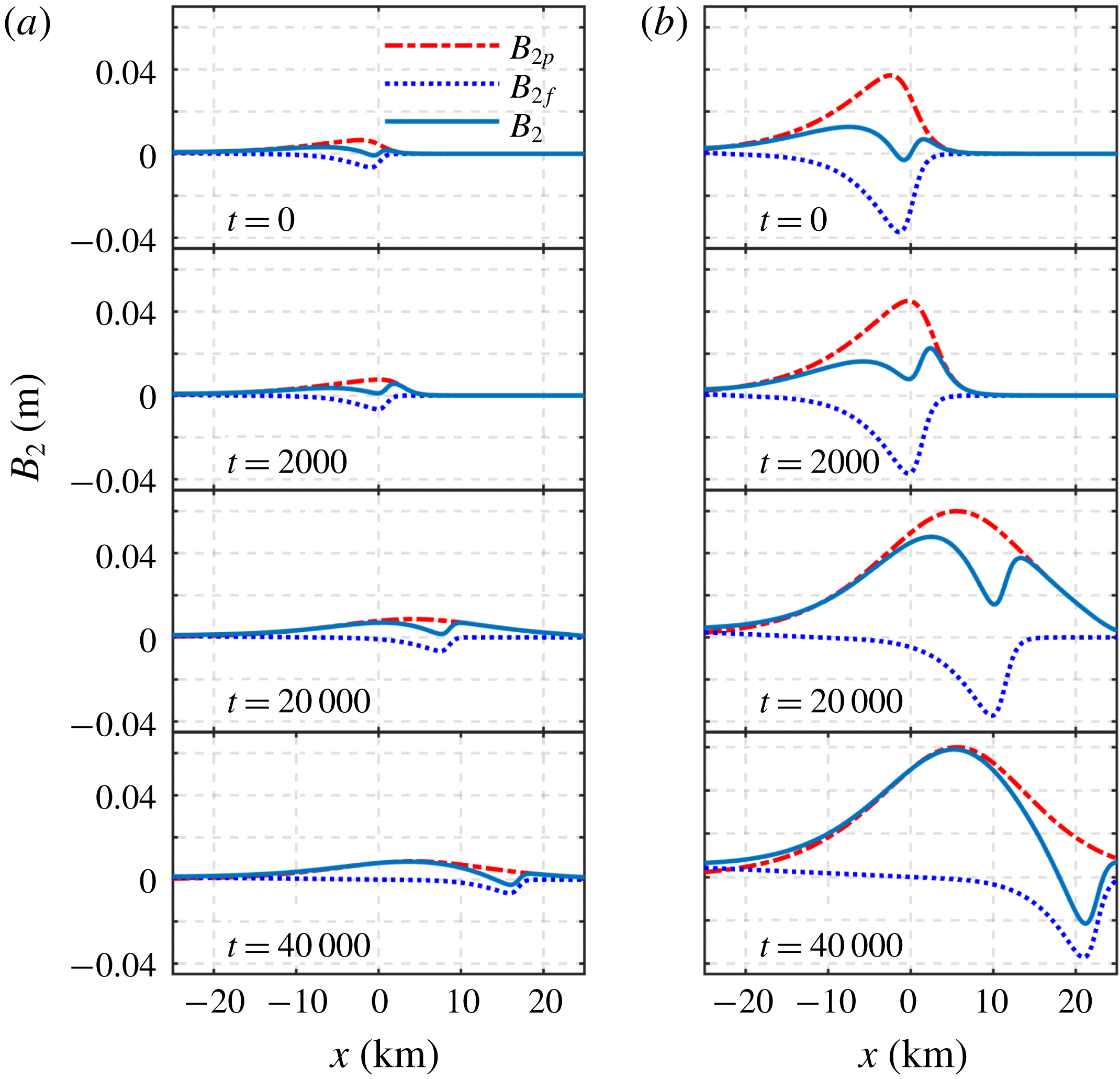
Figure 8 shows the evolution
 $B_{2p},~B_{2f}$
and their summation
 $B_{2}$
, which is similar to the previous case, and also with a four times larger amplitude for the ‘thick (
 $h_{2}=80~\text{m}$
)’ pycnocline case than in the ‘thin (
 $h_{2}=40~\text{m}$
)’ pycnocline case due to the increase in
 $\tilde{\unicode[STIX]{x1D6FE}}$
. The much more striking phenomenon is that the amplitudes in this ‘steep’ slope case are five times larger compared to the ‘gentle’ slope case for both the ‘thin’ and ‘thick’ pycnocline cases. For example, in the ‘thick’ pycnocline case, the peak amplitude for the slaved wave is approximately 0.3 m and
 $-0.12~\text{m}$
for the free wave, while in the ‘gentle’ slope case, they are 0.06 m and
 $-0.03~\text{m}$
, respectively. The same relationships occur for the ‘thin’ pycnocline case. This feature is caused by the larger value of
 $|\unicode[STIX]{x2202}h/\unicode[STIX]{x2202}T_{1}|$
when the slope is steeper. The slaved and free wave amplitudes are proportional to
 $\mp \tilde{\unicode[STIX]{x1D6FE}}(\unicode[STIX]{x2202}h/\unicode[STIX]{x2202}T_{1})a/K$
, and the slope gradient affects the ranges of
 $\unicode[STIX]{x2202}h/\unicode[STIX]{x2202}T_{1}$
, but not those of
 $\tilde{\unicode[STIX]{x1D6FE}}$
,
 $a$
and
 $K$
. Hence, the wave amplitudes are sensitive to the topographic gradient, and change in proportion to the bottom slope changes. In both cases, under the KdV dynamics (see figure 9), the waves form a much stronger rarefaction wave following by an undular bore during their evolution due to the larger initial amplitude, even though the magnitudes of
 $\unicode[STIX]{x1D707}_{2}$
are almost the same as those in the ‘gentle’ slope case.
4 Application: smooth density stratification
As a complement to the three-layer model (3.1) of the previous section, here we examine a case when the background density stratification is smooth and given by a representation of either a ‘thin’ (4.1) or a ‘thick’ (4.2) diffuse pycnocline, respectively:
 $$\begin{eqnarray}\displaystyle & \displaystyle \unicode[STIX]{x1D70C}_{0}(z)=\unicode[STIX]{x1D70C}_{2}+\unicode[STIX]{x0394}\unicode[STIX]{x1D70C}\tanh (1\times 10^{-1}\,(z+150)), & \displaystyle\end{eqnarray}$$
 $$\begin{eqnarray}\displaystyle & \displaystyle \unicode[STIX]{x1D70C}_{0}(z)=\unicode[STIX]{x1D70C}_{2}+\unicode[STIX]{x0394}\unicode[STIX]{x1D70C}\tanh (5\times 10^{-2}\,(z+150)). & \displaystyle\end{eqnarray}$$
There is a superficial resemblance to the three-layer fluid that the density varies from
 $\unicode[STIX]{x1D70C}_{2}-\unicode[STIX]{x0394}\unicode[STIX]{x1D70C}$
in the upper fluid to
 $\unicode[STIX]{x1D70C}_{2}+\unicode[STIX]{x0394}\unicode[STIX]{x1D70C}$
in the lower fluid, with a value of
 $\unicode[STIX]{x1D70C}_{2}$
in the middle at
 $z=-150~\text{m}$
. But there is an essential difference that here the buoyancy frequency
 $N$
has a single maximum at
 $z=-150~\text{m}$
, whereas for the three-layer fluid there is a maximum (formally infinite) at the upper interface
 $z=-h_{1}$
and at the lower interface
 $z=-h_{1}-h_{2}$
. In the numerical calculations that follow, we set
 $\unicode[STIX]{x1D70C}_{2}=1025~\text{kg}~\text{m}^{-3}$
and
 $\unicode[STIX]{x0394}\unicode[STIX]{x1D70C}=1~\text{kg}~\text{m}^{-3}$
. The bottom topography is the same as in § 3, where we use (3.11) for a ‘gentle’ and (3.14) for a ‘steep’ slope gradient variation, respectively. We now examine the mode
 $2$
wave generation in four cases, analogous to those in the previous section, that is, a ‘thin’ or ‘thick’ pycnocline with a ‘gentle’ or ‘steep’ slope gradient.
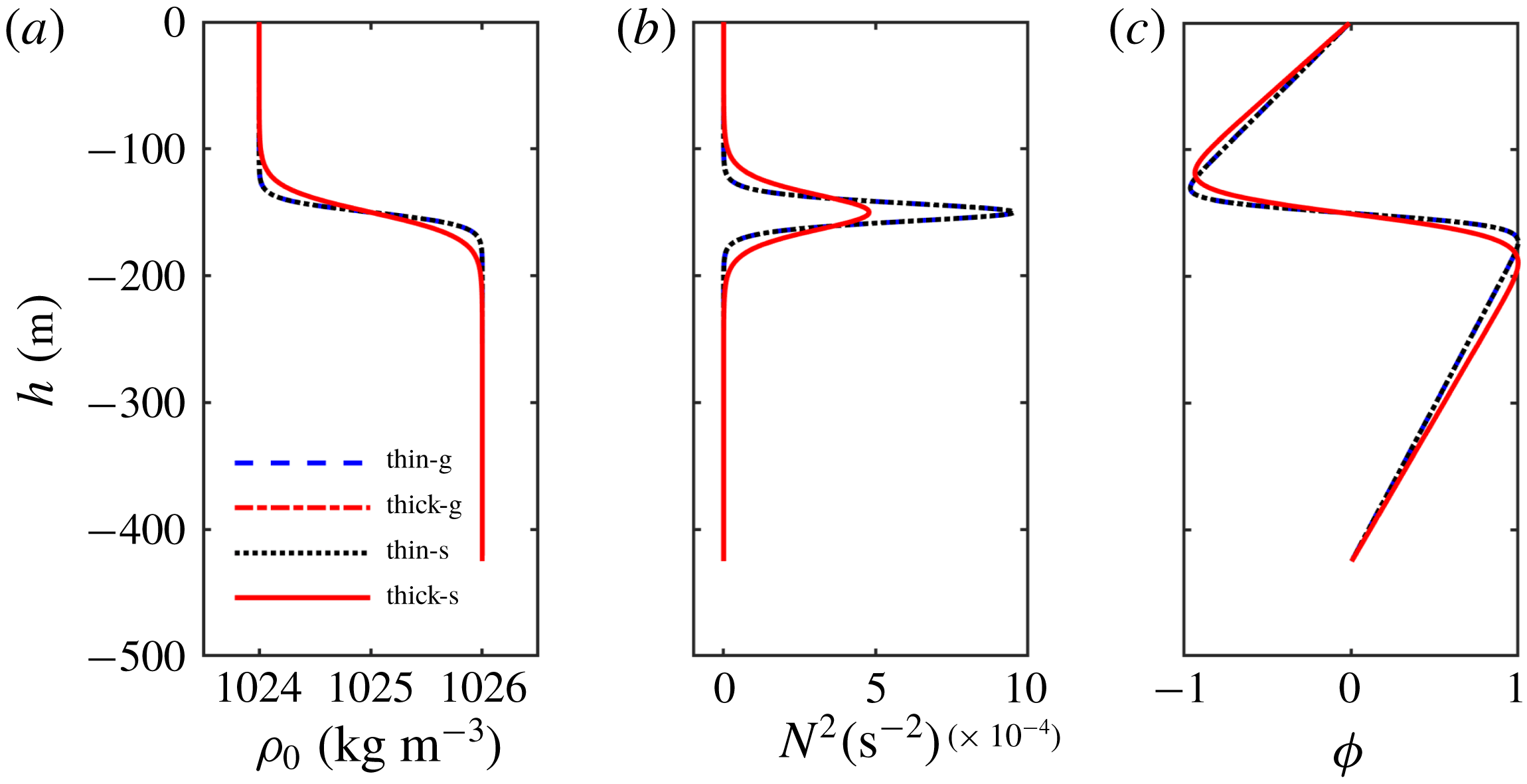
The background environment profiles at the mid-point in the slope-shelf region for the smooth-stratification fluid case: (a) density stratification
 $\unicode[STIX]{x1D70C}_{0}$
; (b) buoyancy frequency represented by
 $N^{2}$
; and (c) modal function
 $\unicode[STIX]{x1D719}$
for mode
 $2$
. Legends ‘thin-g’ and ‘thick-g’ are the ‘thin’ and ‘thick’ pycnocline cases with the ‘gentle’ slope (3.11); ‘thin-s’ and ‘thick-s’ are the ‘thin’ and ‘thick’ pycnocline cases with the ‘steep’ slope (3.14).

Figure 10 shows the background environment profiles for these four cases. These profiles are extracted from the middle point of the slope-shelf region, where the total depths are identical, and so the results are the same (at this point) no matter whether the slope is ‘gentle’ or ‘steep’. Also, the thickness of the middle layer (treated here as the width of
 $N^{2}$
around its maximum value) is approximately doubled in the ‘thick’ pycnocline case compared to the ‘thin’ pycnocline case, with similar values to the three-layer fluid case, where
 $h_{2}=80~\text{m}$
in the ‘thick’ case and
 $h_{2}=40~\text{m}$
in the ‘thin’ case. But note that the calculated modal function
 $\unicode[STIX]{x1D719}(z)$
has the opposite polarity to the modal function of the three-layer fluid, with a maximum of
 $|\unicode[STIX]{x1D719}(z)|$
at the lower interface, even though the estimated
 $h_{1}<h_{3}$
as in the three-layer fluid. This can be attributed to the weak but non-zero stratification in the upper and lower layers.
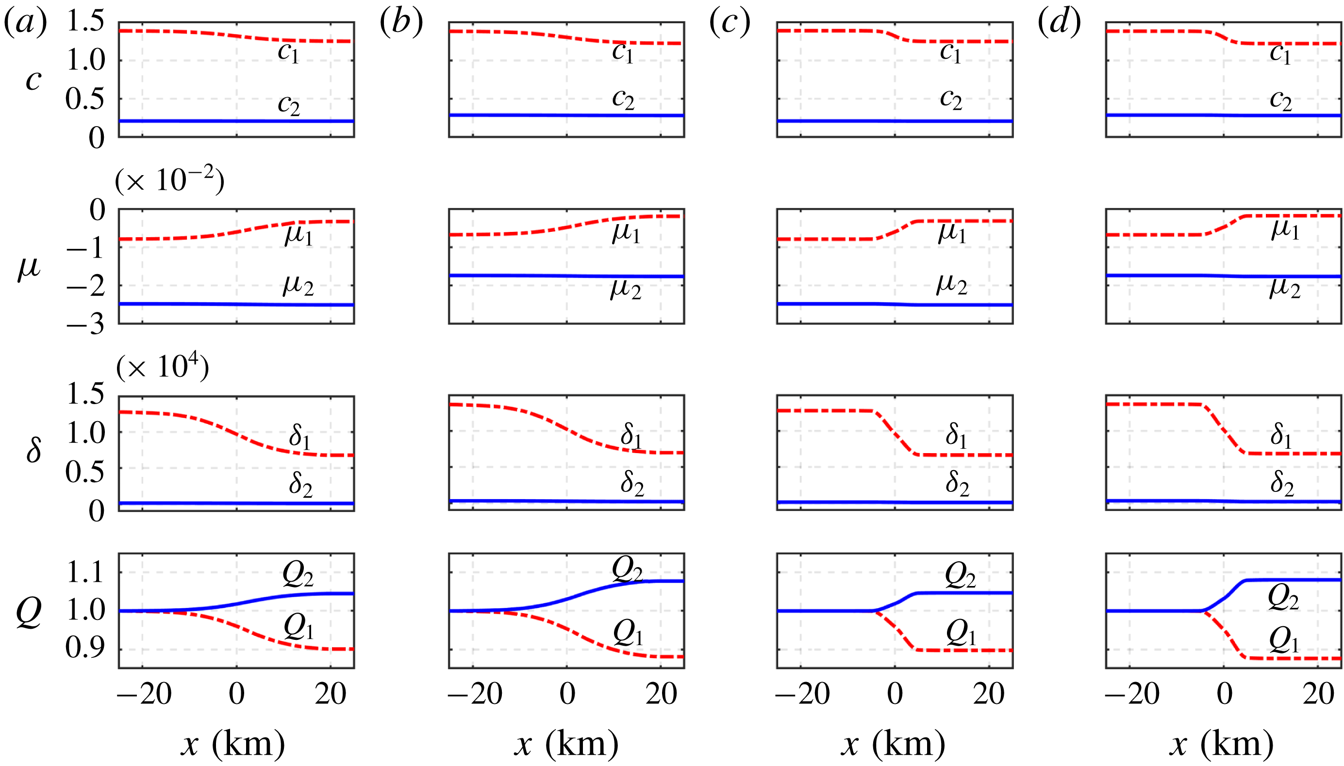
The coefficients of the KdV equation (2.1) for mode 1 and mode 2 waves for the smooth-stratification case. From top to bottom: the phase speeds
 $c_{1,2}$
(m s
 $^{-1}$
), the nonlinear coefficients
 $\unicode[STIX]{x1D707}_{1,2}$
(s
 $^{-1}$
), the dispersive coefficients
 $\unicode[STIX]{x1D6FF}_{1,2}$
(
 $\text{m}^{3}~\text{s}^{-1}$
) and the linear magnification factor
 $Q_{1,2}$
, respectively. (a) The case with ‘gentle’ slope and ‘thin’ middle pycnocline thickness (‘thin-g’); (b) ‘gentle’ slope and ‘thick’ middle pycnocline thickness (‘thick-g’); (c) ‘steep’ slope and ‘thin’ middle pycnocline thickness (‘thin-s’); and (d) ‘steep’ slope and ‘thick’ middle pycnocline thickness (‘thick-s’).

Parameters of the particular (2.39) and free (2.40) solutions in the smooth-stratification case. The expressions
 $\tilde{\unicode[STIX]{x1D6FE}}$
and
 $\unicode[STIX]{x2202}h/\unicode[STIX]{x2202}T_{1}$
in units
 $\text{m}^{-1}$
and
 $\text{m}~\text{s}^{-1}$
, respectively, and the parameters
 $a$
and
 $K$
of the mode 1 solitary wave (2.38) in units
 $\text{m}$
and
 $\text{m}^{-1}$
, respectively. Panels (a–d) are for the same conditions as in figure 11.

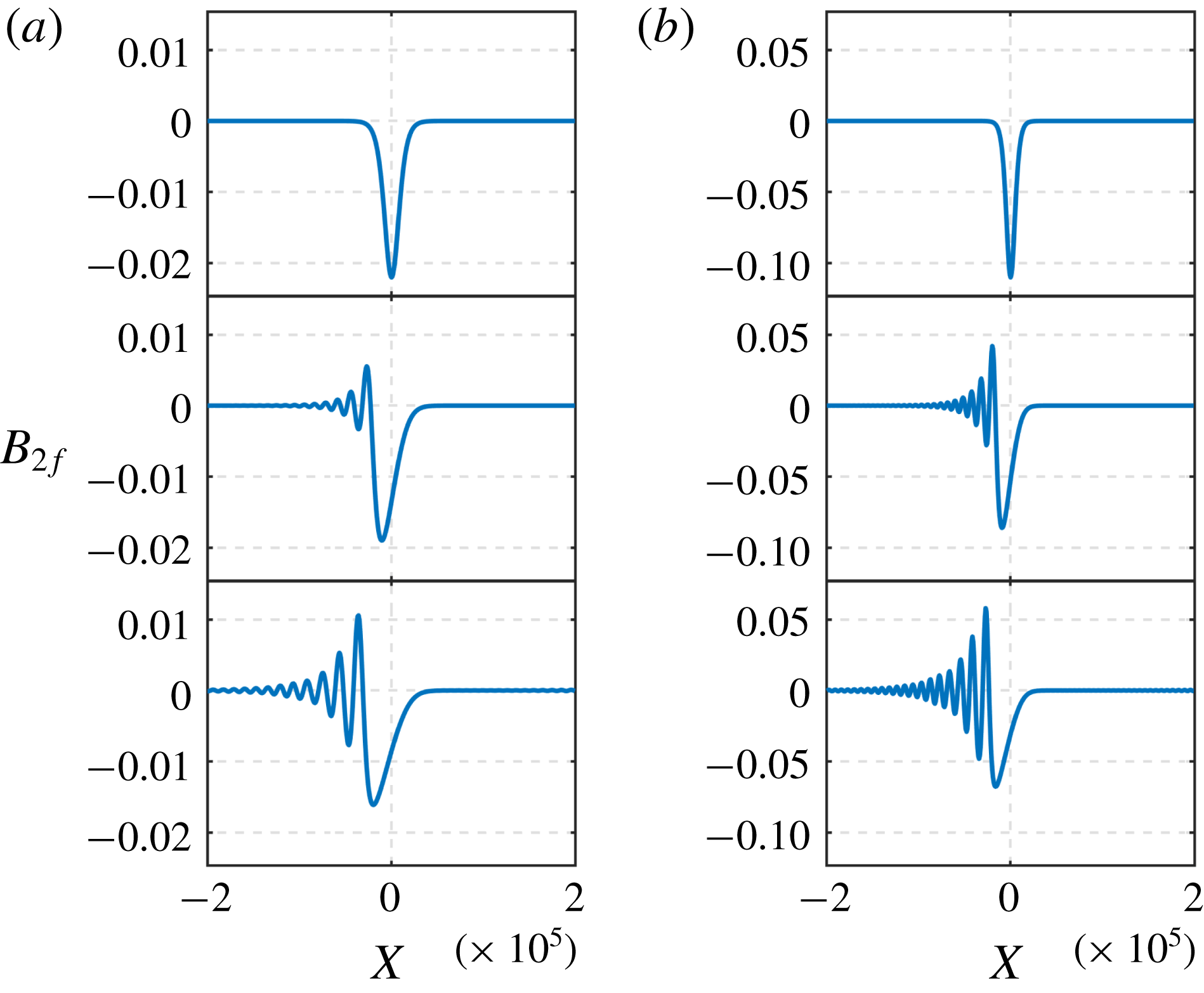
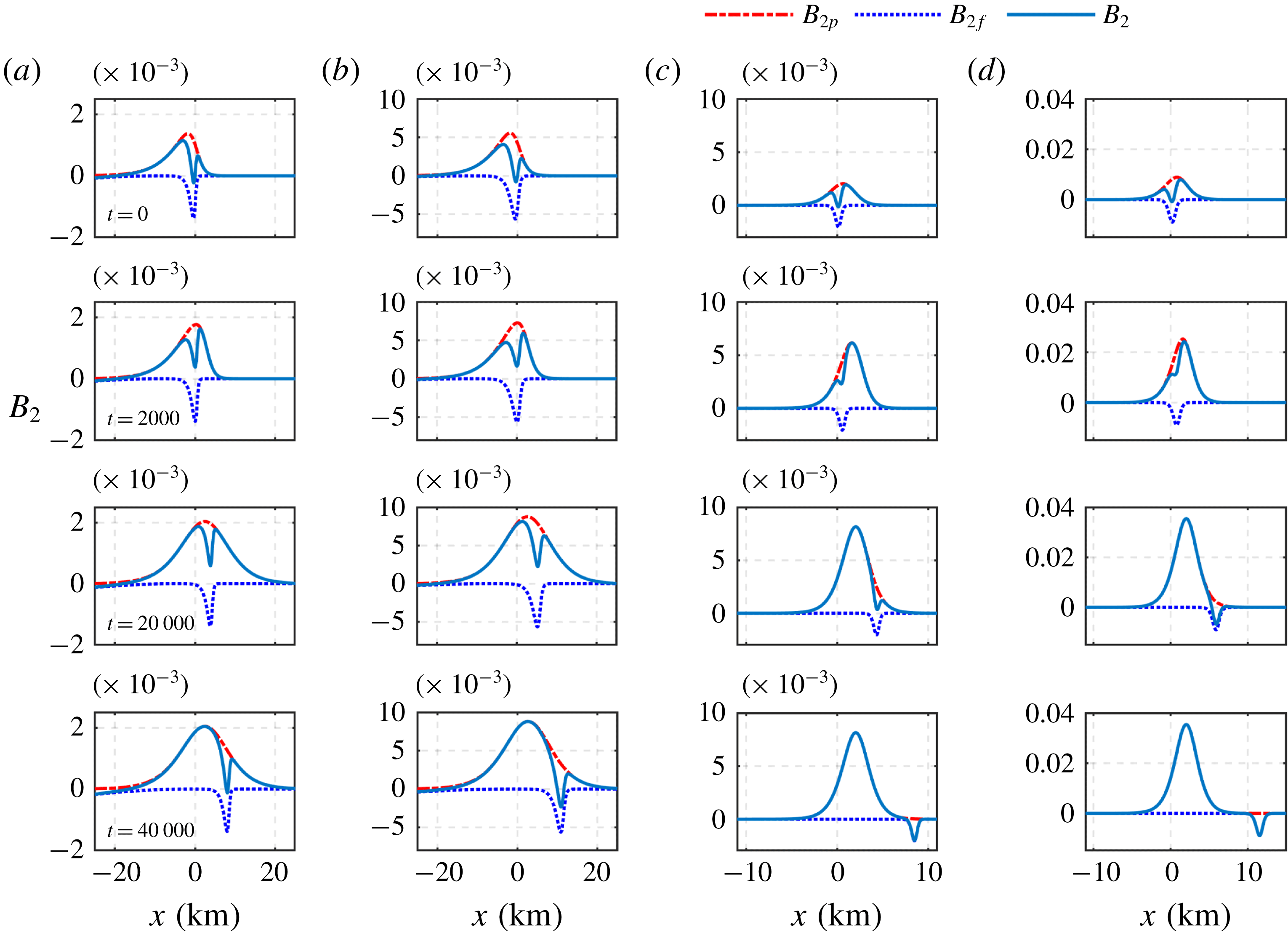
Plots of the slaved wave (2.39) and the free wave (2.40) as time increases for the smooth-stratification case, From top to bottom, they are spatial plots for each fixed
 $t$
, with
 $t$
varying from
 $0$
to 40 000 s. Panels (a–d) are for the same conditions as in figure 11. Note the horizontal axis labels for panels (c,d) are the same as (a,b), but only a part is shown.

Plots of the evolution of the free mode 2 wave under KdV dynamics (3.12) with the initial condition (3.13) for the smooth-stratification case. From top to bottom, the distances from the initial point are 0 km, 25 km and 50 km, respectively. Panels (a)–(d) are for the same conditions as in figure 11.

Figure 11 shows the coefficients of the KdV equation (2.1) for mode 1 and mode 2 waves under this smooth-stratification case. Panels (a,b) are for the ‘gentle’ slope (3.11) with (a) ‘thin’ and (b) ‘thick’ middle layer thickness, respectively; while panels (c,d) are for the ‘steep’ slope (3.14) with (c) ‘thin’ and (d) ‘thick’ pycnoclines. Overall, these results are consistent with those in figures 2 and 6 for the three-layer cases. However, importantly, the mode 2 phase speed
 $c_{2}$
is only one-half of that in the three-layer fluid case, and the nonlinear coefficients
 $\unicode[STIX]{x1D707}_{2}$
have the opposite sign due to the aforementioned opposite polarity of the modal function (see figure 10
c).
Figure 12 shows the parameters of the particular (2.39) and free (2.40) waves in these four different cases. Comparing with the analogous figures 3 and 7 for the three-layer fluid, we see that
 $\unicode[STIX]{x2202}h/\unicode[STIX]{x2202}T_{1}$
,
 $a$
and
 $K$
are almost in the same range and variation trend, but
 $\tilde{\unicode[STIX]{x1D6FE}}$
is
 $10$
times smaller than that in the three-layer fluid system. The reason is that the mode 2 phase speed
 $c_{2}$
is much smaller than that in the three-layer fluid case, although
 $c_{1}$
is comparable; see (2.9) and (2.31). Figure 13 shows the plots of the slaved and free waves as time increases in these different conditions. Here figure 13(a–d) are the results in the corresponding four cases in figure 12. Comparing with figures 4 and 8, we see that the mode 2 wave evolution in this smooth-stratification case is qualitatively consistent with that in the three-layer fluid case. But the generated slaved and free mode 2 wave amplitudes are now
 $10$
times smaller, corresponding to the smaller coefficient
 $\tilde{\unicode[STIX]{x1D6FE}}$
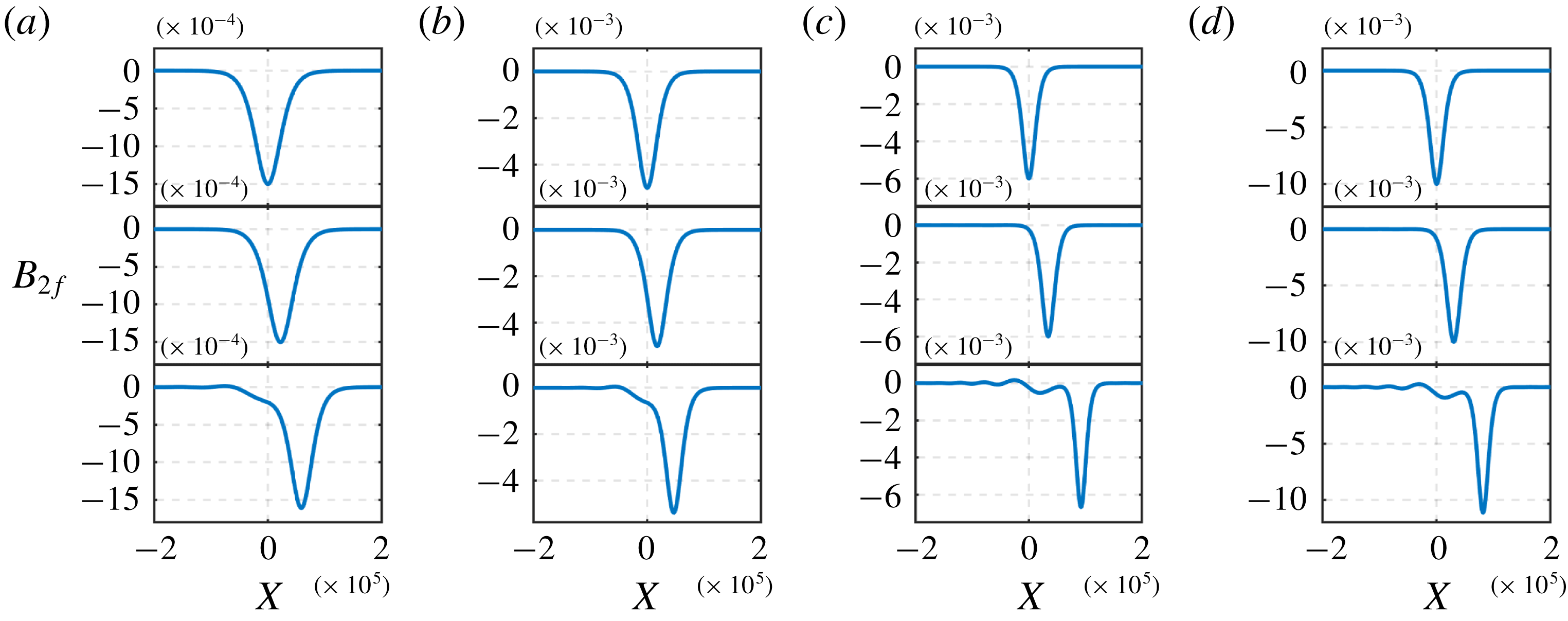
in figure 12. Figure 14 shows the evolution of the free mode
 $2$
wave under KdV dynamics (3.12) and is now quite different from the results in the three-layer fluid system; see figures 5 and 9. The reason is that now the nonlinear coefficient
 $\unicode[STIX]{x1D707}_{2}<0$
and so solitary waves have the same sign as the initial condition for the free mode 2 wave. Hence wave fission occurs instead of the formation of a rarefaction wave with a trailing undular bore. The initial free mode 2 wave is convex here for this smooth-stratification case, whereas in the three-layer case, the initial free mode 2 wave is concave.
We find that here, as in the three-layer fluid case, the generated mode 2 wave amplitude is mainly associated with the pycnocline thickness and the slope gradient. The mode 2 wave amplitudes in figures 14(b) and 14(d) are approximately four times larger than in figures 14(a) and 14(c), respectively, which is the square of the difference of the pycnocline thickness; also, the amplitudes in figures 14(c) and 14(d) are approximately four times larger than in figures 14(a) and (b), respectively, close to the slope gradient discrepancy. These outcomes are consistent with those using the three-layer fluid of § 3. We conclude that the pycnocline thickness and the bottom topography gradient can be expected to play important roles in the magnitude of the generated mode 2 wave amplitude. But, as noted, the smooth-stratification case reduces
 $\tilde{\unicode[STIX]{x1D6FE}}$
due to the smaller ratio
 $c_{2}/c_{1}$
and hence reduces the generated amplitudes, indicating that sharp interfaces induce stronger mode
 $2$
waves.
5 Application: ocean examples
In this section, we examine two oceanic cases, the New Jersey continental shelf (Shroyer et al. Reference Shroyer, Moum and Nash2010) and the South China Sea (Liu et al. Reference Liu, Su, Hsu, Kuo and Ho2013), where mode 2 waves have been reported. In both these regions, internal solitary waves (both mode 1 and mode 2) occur frequently and in situ data are available. In particular, the mode 2 wave recorded by Liu et al. (Reference Liu, Su, Hsu, Kuo and Ho2013) (see figure 1) seems likely to have been generated by mode 1 waves, under the mechanism discussed here. The generation mechanism of the mode 2 waves documented by Shroyer et al. (Reference Shroyer, Moum and Nash2010) may be related to frontal intrusions or tidal forcing near the shelf break and may not be due to a mode 1 wave interaction with topography. However, the mechanism for the generation of the mode 2 waves is not settled and so the clear in situ data of Shroyer et al. (Reference Shroyer, Moum and Nash2010) allow us to test the present analysis as an alternative mechanism for mode 2 wave generation on the New Jersey continental shelf.
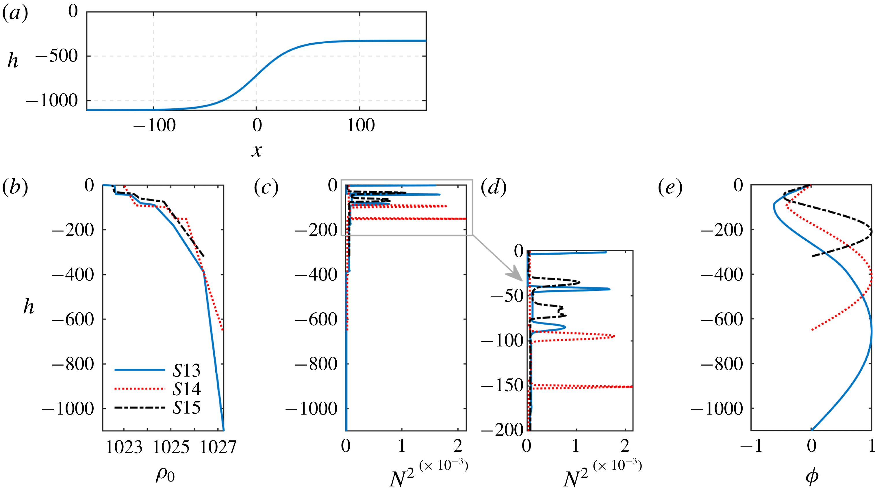
5.1 New Jersey continental shelf
Mode 1 and mode 2 nonlinear internal waves were documented by Shroyer et al. (Reference Shroyer, Moum and Nash2010) and Shroyer, Moum & Nash (Reference Shroyer, Moum and Nash2011) through both mooring and ship-tracked records obtained over New Jersey continental shelf in the summer of 2006, during the Office of Naval Research’s Nonlinear Internal Wave Initiative–Shallow Water ’06 experiment (NLIWI-SW06). The nonlinear internal waves had a typical amplitude of
 $-8~\text{m}$
during most of the time of the observation month, but the displacement could exceed
 $-15~\text{m}$
over some periods of that month. One mode 2 wave train was detected during NLIWI-SW06 by shipboard records, and was referred to as Wave Jasmine, due to a naming convention for ship-tracked waves (see Shroyer et al.
Reference Shroyer, Moum and Nash2010). This mode 2 wave train (Wave Jasmine) was documented by three detailed profiling periods (denoted as 3a, 3b and 3c here, in order to be consistent with Shroyer et al. (Reference Shroyer, Moum and Nash2010), who showed these three profiles in their figure 3a, 3b and 3c). The first and second profiling series consisted of three mode 2 waves, while the third transect only had two mode 2 waves with a small mode 1 wave tail. The amplitudes of these waves were defined by taking the sum of a half of the maximum density displacement above and below the pycnocline, and was near 4 m in the first and third periods and 3 m in the second transect. The average wave speed obtained from the ship record measurements was approximately
 $0.48~\text{m}~\text{s}^{-1}$
, which was slightly larger than the mode 2 linear phase speed calculated from the modal equation that showed an increase from
 $0.4~\text{m}~\text{s}^{-1}$
to
 $0.46~\text{m}~\text{s}^{-1}$
, under the effects of background shear.
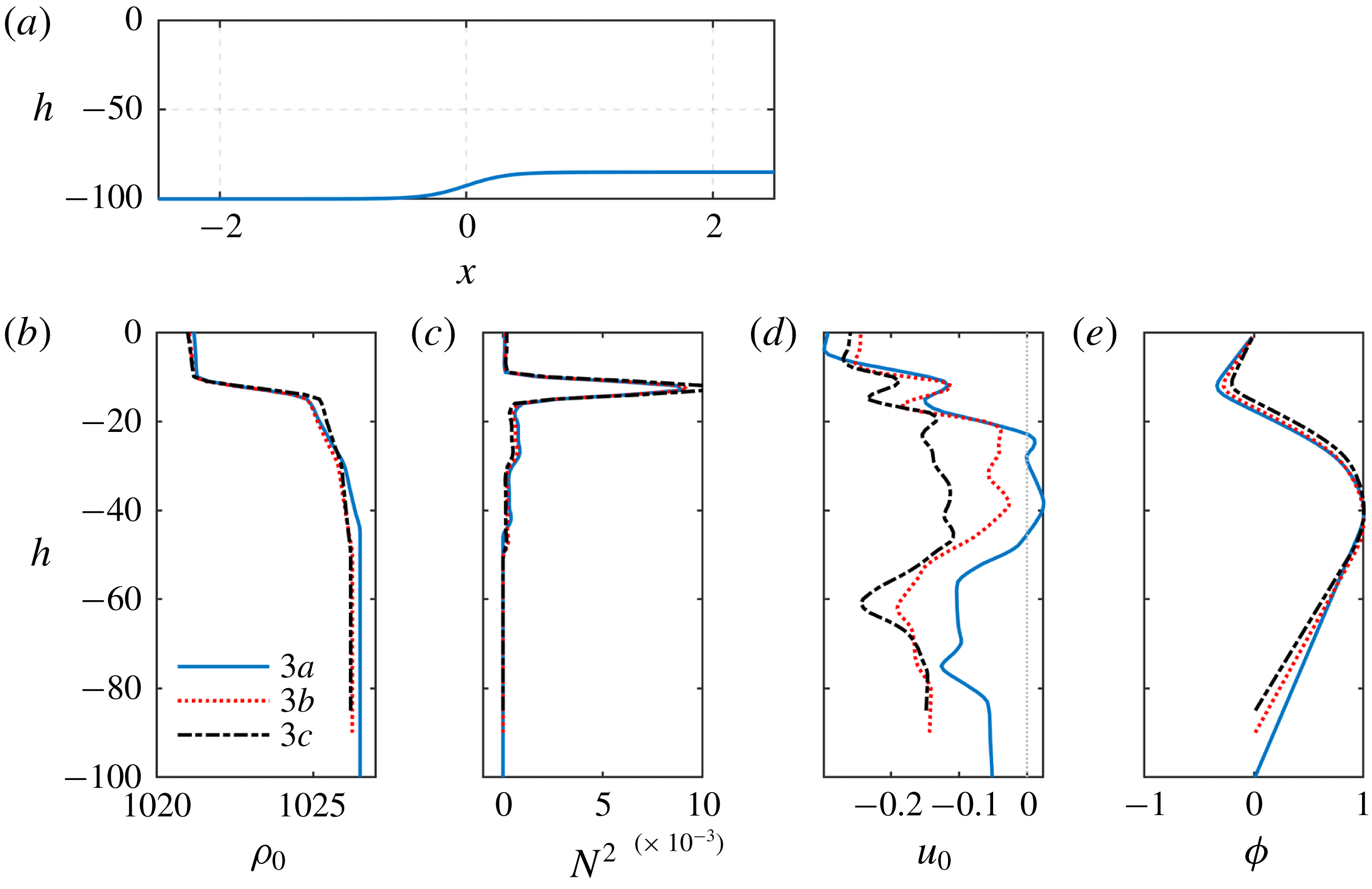
The background environment profiles for the New Jersey continental shelf case. (a) The depth
 $h$
(m) along the slope-shelf region
 $x$
(km), see (5.1); (b) density stratification
 $\unicode[STIX]{x1D70C}_{0}~(\text{kg}~\text{m}^{-3})$
; (c) buoyancy frequency represented by
 $N^{2}$
(
 $\text{s}^{-2}$
); (d) velocity
 $u_{0}$
(
 $\text{m}~\text{s}^{-1}$
); and (e) calculated vertical structure
 $\unicode[STIX]{x1D719}$
(in unit of 1); as shown in Shroyer et al. (Reference Shroyer, Moum and Nash2010), figures 4 and 5. Here 3a, 3b and 3c represent the first, second and third profiling series for Wave Jasmine documented by Shroyer et al. (Reference Shroyer, Moum and Nash2010).

The depth variation along the wave propagation path was not given, but we can estimate this from the density profiles at the three profiling points (100 m, 90 m and 85 m) and then set it to be
 $$\begin{eqnarray}\displaystyle h(x)=92.5-7.5\tanh (3\times 10^{-3}x) & & \displaystyle\end{eqnarray}$$
(see figure 15). The slope variation here is very smooth and gentle, as the depth changes from 100 m to 85 m over a horizontal distance greater than 3 km. This may not be very realistic and may lead to an inconsistent predicted wave amplitude in comparison to the observed mode 2 wave amplitude, recalling that we have found that the mode 2 amplitude is sensitive to the topographic gradient. We extracted the data generated of the background density and currents (see figure 15) at the above three ship-tracked profiling periods (3a, 3b and 3c) from Shroyer et al. (Reference Shroyer, Moum and Nash2010), figure 4, and then calculated the buoyancy frequency and the modal function (note our solution is normalised by
 $\max [\unicode[STIX]{x1D719}]=1$
); see figure 15, which is consistent with the results in figure 4(b) and figure 5 in Shroyer et al. (Reference Shroyer, Moum and Nash2010).
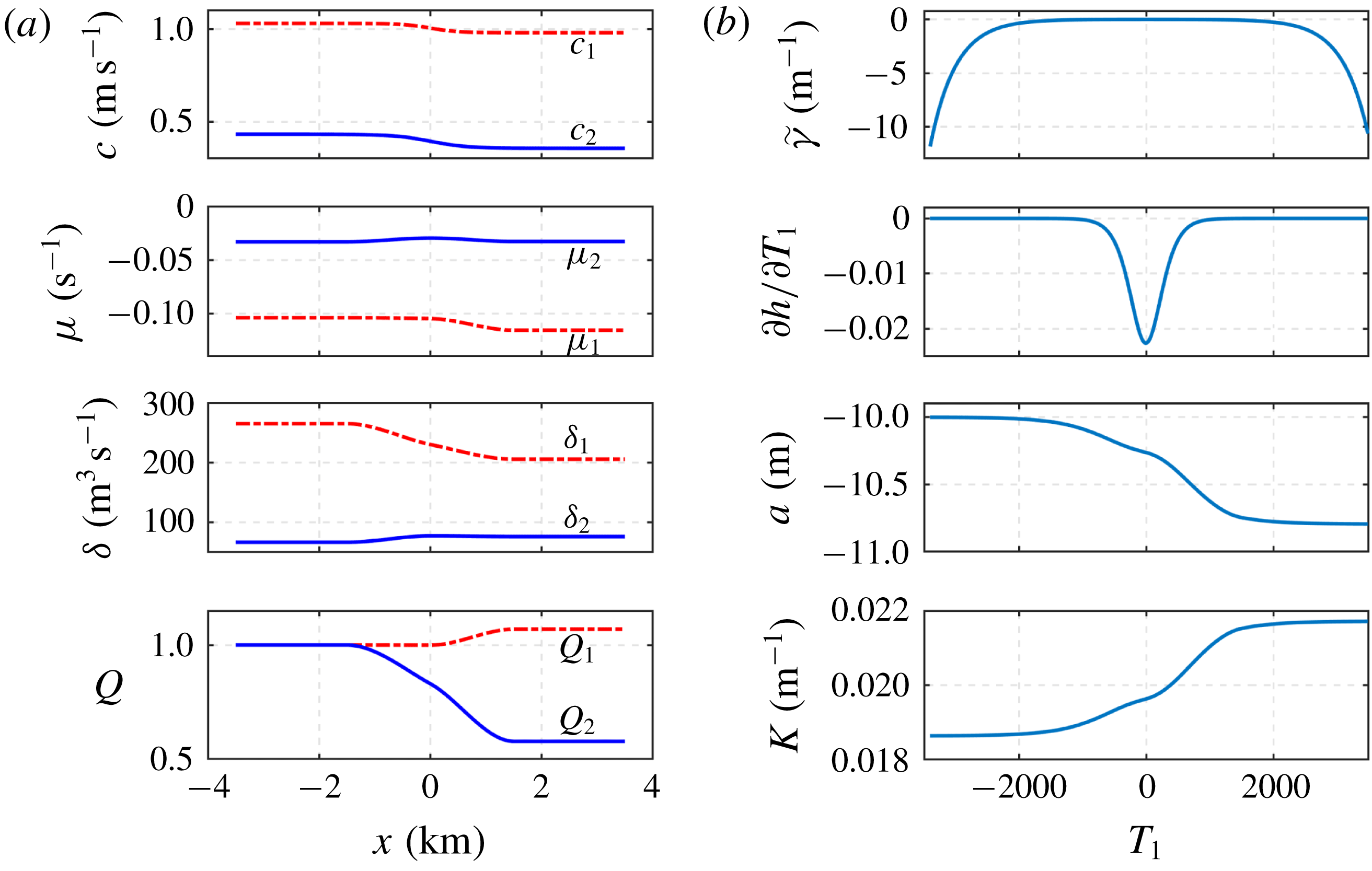
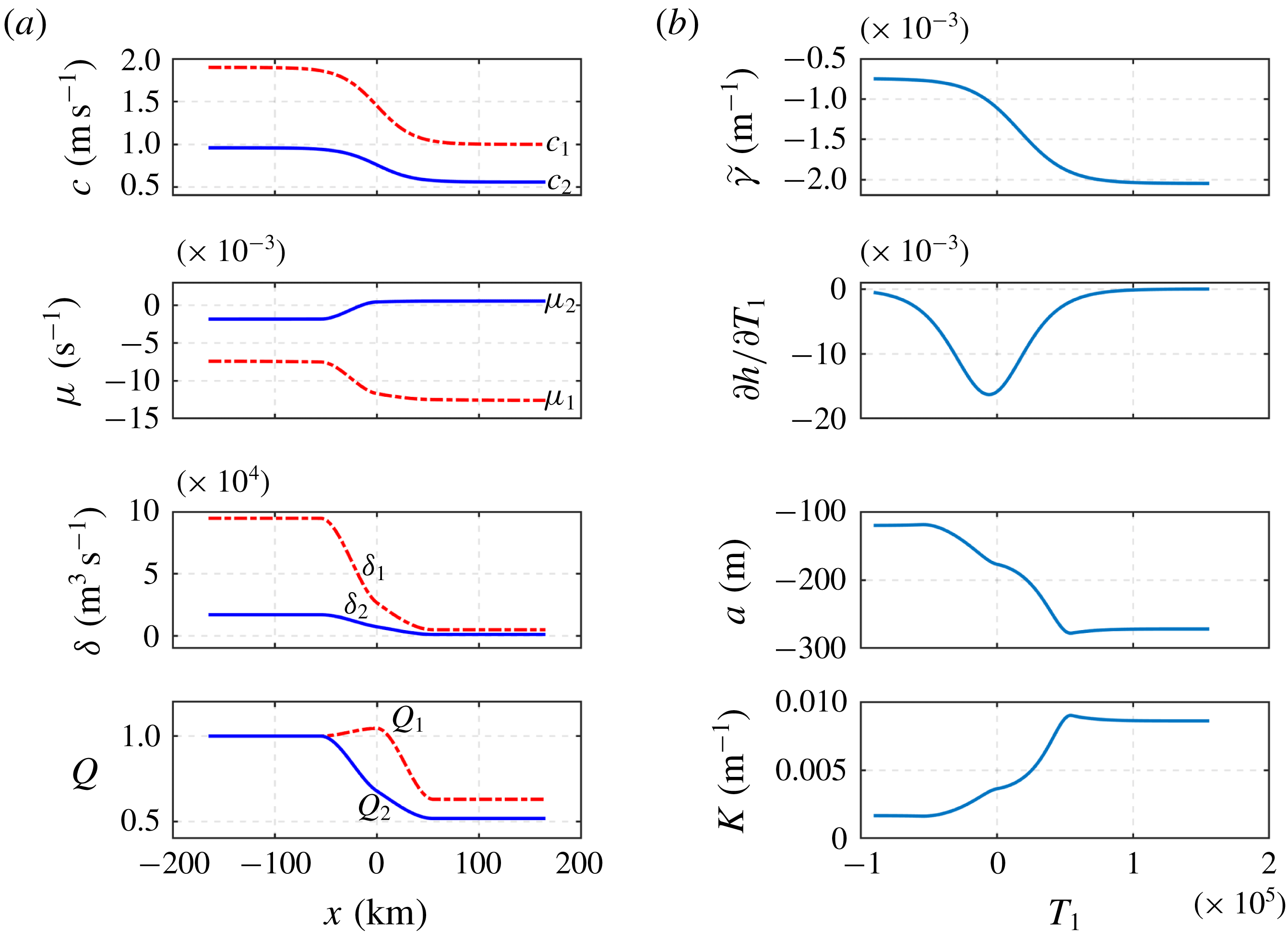
(a) The KdV coefficients (
 $c,\unicode[STIX]{x1D707},\unicode[STIX]{x1D6FF},Q$
) for mode 1 and mode 2 solitary waves and (b) parameters (
 $\tilde{\unicode[STIX]{x1D6FE}},\unicode[STIX]{x2202}h/\unicode[STIX]{x2202}T_{1},a,K$
) for the New Jersey continental shelf case.

Figure 16 shows the KdV coefficients
 $c$
,
 $\unicode[STIX]{x1D707}$
,
 $\unicode[STIX]{x1D6FF}$
and
 $Q$
calculated from (2.2), (2.3), (2.4) and (2.5) for mode 1 and mode 2 solitary waves (figure 16
a) and parameters
 $\tilde{\unicode[STIX]{x1D6FE}}$
,
 $\unicode[STIX]{x2202}h/\unicode[STIX]{x2202}T_{1}$
,
 $a$
and
 $K$
with respect to
 $T_{1}$
for linear theory (figure 16
b). Both
 $c_{1}$
and
 $c_{2}$
decrease along the transect, with ranges
 $1.03{-}0.98$
m s
 $^{-1}$
and
 $0.43{-}0.36$
m s
 $^{-1}$
, respectively. The variation trend of
 $c_{2}$
is slightly smaller than and opposite to the theoretical results of Shroyer et al. (Reference Shroyer, Moum and Nash2010) (
 $0.4{-}0.46$
m s
 $^{-1}$
). Here
 $\unicode[STIX]{x1D707}_{1}$
and
 $\unicode[STIX]{x1D707}_{2}$
are negative over the slope, indicative that there is no polarity change and that only a depression mode 1 wave and convex mode 2 wave can exist. From figure 16(b), we can see that the mode 1 initial solitary wave amplitude is
 $a_{0}=-10~\text{m}$
and we recall that the amplitudes for both the slaved and free wave are related to the magnitude of
 $\pm 2\tilde{\unicode[STIX]{x1D6FE}}(\unicode[STIX]{x2202}h/\unicode[STIX]{x2202}T_{1})a/K$
, which is
 $O(-2)$
.
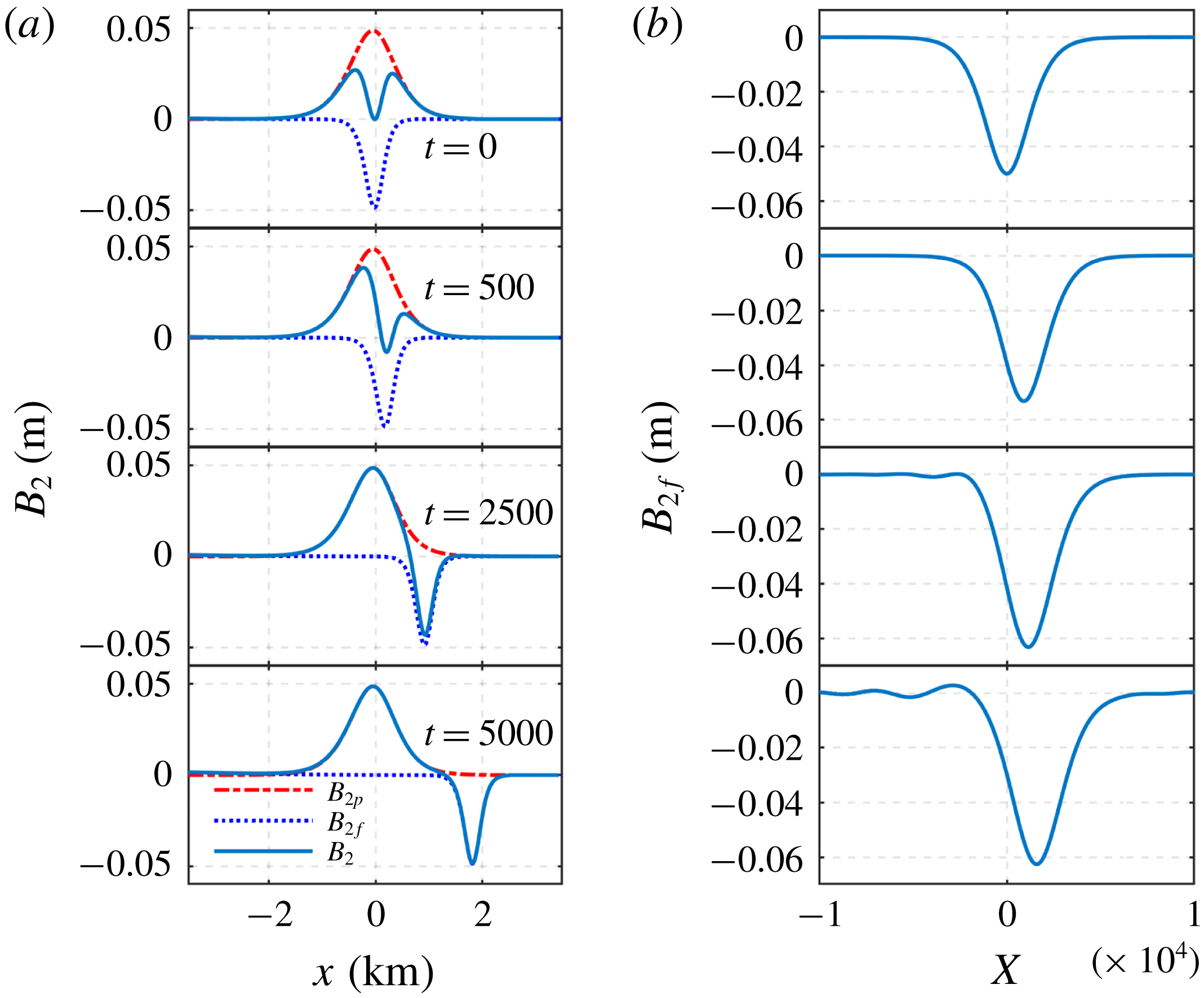
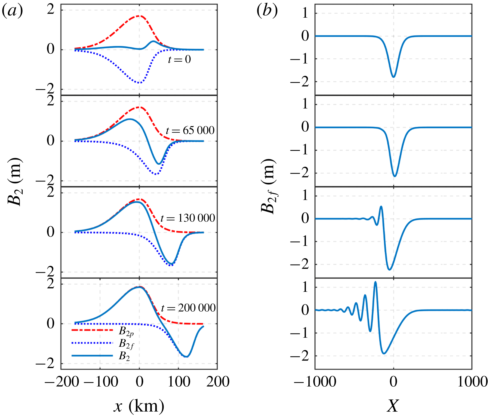
Mode 2 wave evolution in the New Jersey continental shelf case. Panel (a) is for the linear theory and (b) is the mode 2 free wave evolution based on the KdV theory.

Figure 17 shows the mode 2 wave evolution both from the linear theory (figure 17
a) and the KdV model (figure 17
b). The slaved wave mode 2 and the free wave mode 2 with amplitude approximately
 $-0.05~\text{m}$
travel with speed
 $c_{1}$
and
 $c_{2}$
, respectively. The slaved wave, which has a wider shape than the free wave, stops when the forcing mode 1 wave reaches around the mid-shelf, where the depth has become shallower. The KdV dynamics then show that the initially convex mode 2 free wave grows slightly from
 $-0.05~\text{m}$
to
 $-0.08~\text{m}$
during the propagation, and then begins to show signs of fission. The simulation with the KdV model is consistent with the observed wave evolution by Shroyer et al. (Reference Shroyer, Moum and Nash2010), although the observed trailing mode 1 wave tail is beyond the scope of this KdV model. The predicted mode 2 wave amplitude (
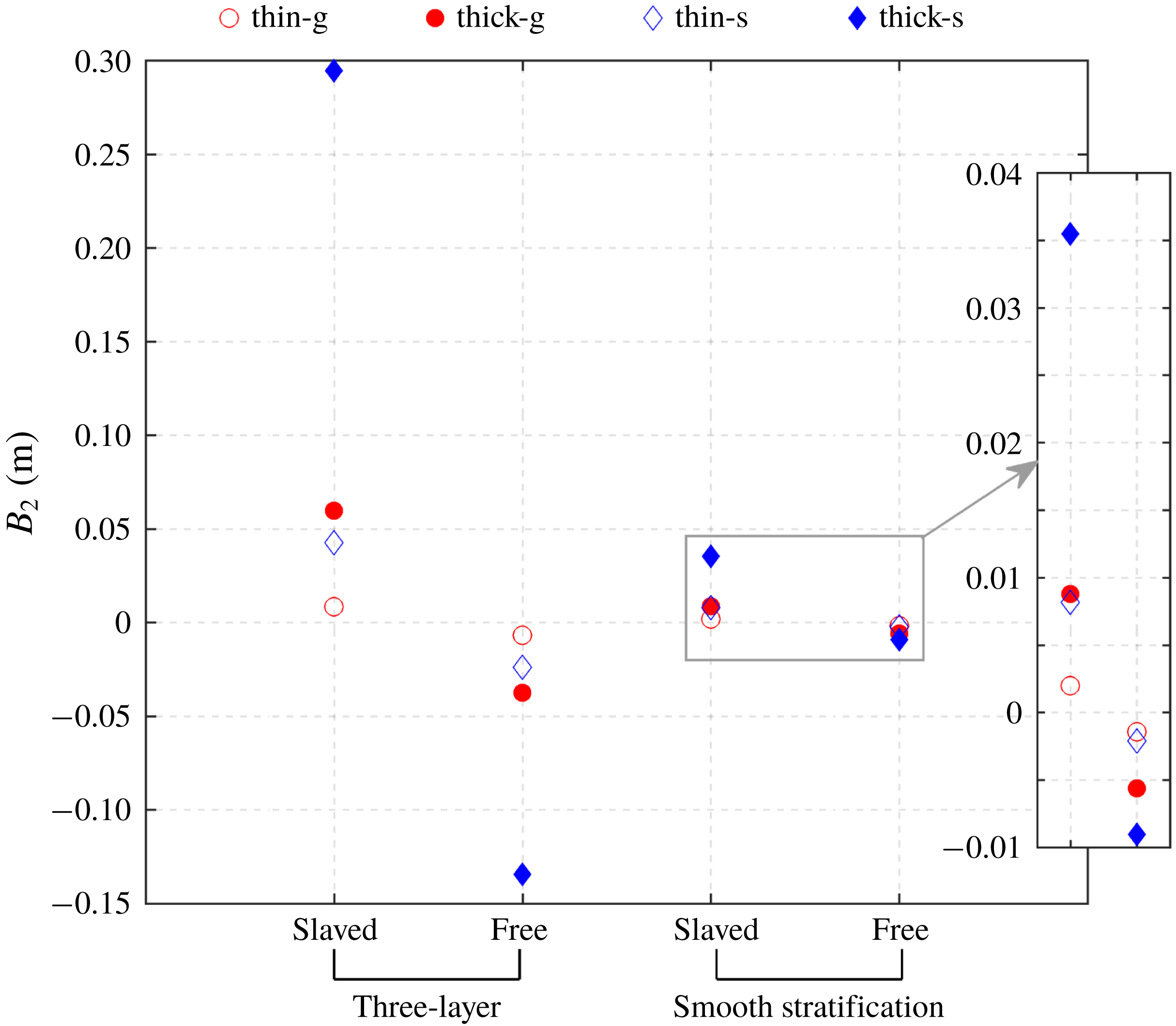
 $-0.05~\text{m}$
) from our linear theory is, however, very different from the observed mode 2 amplitude of
 $-3~\text{m}$
. This would imply that the observed mode 2 waves in this region are not generated from a mode 1 wave incident on the topography and is consistent with the comments in Shroyer et al. (Reference Shroyer, Moum and Nash2010), who suggest that in this case the mode 2 waves may have been generated by a density intrusion.
5.2 South China Sea
Although mode 2 internal solitary waves are less often observed in comparison to mode 1 waves, they were documented by Yang et al. (Reference Yang, Fang, Chang, Ramp, Kao and Tang2009) on the continental shelf of the northern South China Sea in both summer and winter, with notable seasonal difference. They showed mode 2 waves were less active in summer than in winter (mode 1 waves in contrast to mode 2), with smaller amplitude and longer time scales, and
 $90\,\%$
of the recorded mode 2 waves appeared after mode 1 internal solitary waves in summer. In winter
 $72\,\%$
arose without mode 1 waves. These observations suggest that the generation mechanisms of mode 2 waves have a seasonal difference, and may be associated with mode 1 waves in summer.
A short intensive field experiment to search for mode 2 waves was made near Dong-Sha Island in the northeastern South China Sea in May 2009, and a mode 2 wave with amplitude 30 m was observed following a large mode 1 wave of amplitude 120 m. Owing to the lack of CTD (conductivity–temperature–depth) data during this field observation, the background oceanographic conditions were obtained from a joint hydrographic survey in May 2006, which covered a larger area containing the location where the above mode 2 waves were documented. Three CTD stations S13, S14, S15 across the shelf break in the middle of this survey area were chosen for the parametric study of mode 2 waves in Liu et al. (Reference Liu, Su, Hsu, Kuo and Ho2013). Here we use the same names S13, S14, S15 to represent the environment parameter information of these three stations.
Liu et al. (Reference Liu, Su, Hsu, Kuo and Ho2013) show the background stratification at these three equally spaced CTD stations (S13, S14, S15), spanning
 $1^{\circ }$
of longitude, which covered 55 km. The depth at each station was recorded as 1100 m, 650 m and 320 m, and so we set the depth to be
 $$\begin{eqnarray}\displaystyle h(x)=715-390\tanh (2.8\times 10^{-5}x) & & \displaystyle\end{eqnarray}$$
(see figure 18). Again this depth may not represent the actual depth, and hence may affect our predicted wave amplitudes. Similarly, we extracted the data of background density (
 $\unicode[STIX]{x1D70C}_{0}$
) from figure 15 in Liu et al. (Reference Liu, Su, Hsu, Kuo and Ho2013) and then calculated the buoyancy frequency (
 $N^{2}$
) and modal function (
 $\unicode[STIX]{x1D719}$
) as in the New Jersey case. From figure 18, we see the buoyancy frequency is consistent with that shown in figure 15 in Liu et al. (Reference Liu, Su, Hsu, Kuo and Ho2013), and the modal function plot shows that the depth of the largest displacements becomes shallower along the wave path.
The background environment profiles for the South China Sea case. (a) The depth
 $h$
(m) along the slope-shelf region
 $x$
(km), see (5.2); (b) density stratification
 $\unicode[STIX]{x1D70C}_{0}~(\text{kg}~\text{m}^{-3})$
; (c,d) buoyancy frequency represented by
 $N^{2}$
(
 $\text{s}^{-2}$
), (d) is the enlarged view for the top 200 m; and (e) modal function
 $\unicode[STIX]{x1D719}$
(in unit of 1); as shown in Liu et al. (Reference Liu, Su, Hsu, Kuo and Ho2013), figure 15. Here S13, S14, S15 represent three different CTD stations during the joint hydrographic survey in May 2006 (Liu et al.
Reference Liu, Su, Hsu, Kuo and Ho2013).

(a) The KdV coefficients (
 $c,\unicode[STIX]{x1D707},\unicode[STIX]{x1D6FF},Q$
) for mode 1 and mode 2 solitary waves and (b) parameters (
 $\tilde{\unicode[STIX]{x1D6FE}},\unicode[STIX]{x2202}h/\unicode[STIX]{x2202}T_{1},a,K$
) for the South China Sea case.

The KdV coefficients for mode 1 and mode 2 waves and the parameters of our linear theory are calculated as in the case above, but without the background current, and are shown in figure 19. Both mode 1 and mode 2 linear long-wave phase speed
 $c_{1}$
and
 $c_{2}$
have the same magnitude and variation trend compared to the results in table 3 in Liu et al. (Reference Liu, Su, Hsu, Kuo and Ho2013), and
 $c_{2}$
is approximately half of
 $c_{1}$
. The nonlinear coefficients
 $\unicode[STIX]{x1D707}_{1}$
and
 $\unicode[STIX]{x1D707}_{2}$
(from the background density field shown in figure 18) differ from their results. The pycnocline is not ‘near-surface’ along the whole transect, and
 $\unicode[STIX]{x1D707}_{1}<0$
throughout, implying a depression mode 1 wave. The coefficient
 $\unicode[STIX]{x1D707}_{2}$
changes sign from negative to positive along the transect, while throughout the modal function has its maximum at the lower interface. Thus for the mode 2 wave evolution, the wave is convex at first and then evolves into a concave form. Figure 18(a) shows parameters of our linear theory, setting the initial mode 1 wave amplitude
 $a_{0}=-120~\text{m}$
, and we see that the mode 2 wave amplitude depends on
 $\pm 2\tilde{\unicode[STIX]{x1D6FE}}(\unicode[STIX]{x2202}h/\unicode[STIX]{x2202}T_{1})a/K$
and is of order of unity. Similarly, the slope is even smoother and gentler than it in the case above, with the largest variation
 $\unicode[STIX]{x2202}h/\unicode[STIX]{x2202}T_{1}$
smaller than
 $-0.02$
.
Mode 2 wave evolution for the South China Sea case. Panel (a) is for the linear theory and (b) is the mode 2 free wave evolution based on the KdV theory.

Figure 20 shows the mode 2 wave evolution from the linear theory (figure 20
a) and the KdV model (figure 20
b). The slaved mode 2 wave of the linear theory evolves with a speed
 $c_{1}$
unchanged in form until the forcing mode 1 wave reaches the shallow water. The free mode 2 wave with amplitude approximately 2 m travels with speed
 $c_{2}$
with a steep front initially but then the rear part accelerates and the wave shape becomes more symmetric. The KdV dynamics show that the initially convex mode 2 free wave grows slightly during propagation, but then at the change of polarity forms a depression rarefaction wave with a trailing undular bore. The mode 2 wave amplitude predicted here (
 $-2~\text{m}$
) is 10 times smaller than the observed one (
 $-30~\text{m}$
) in the South China Sea by Liu et al. (Reference Liu, Su, Hsu, Kuo and Ho2013). A partial explanation may follow by recalling that the wave amplitude in this linear theory depends on the gradient of the slope. The resolution of the in situ topographic data here is quite rough, with 55 km increments, and hence may not resolve the steeper gradients. Furthermore, the amplitude reported by Liu et al. (Reference Liu, Su, Hsu, Kuo and Ho2013) was estimated from temperature data, which may not necessarily be the same as the wave amplitude defined here based on the normalised modal function. Finally, we note that the background density profile we have used in figure 18, taken from Liu et al. (Reference Liu, Su, Hsu, Kuo and Ho2013), is at a different time from their observation of the mode 2 wave.
6 Discussion
In this paper, we have examined the possible generation of mode 2 waves by the interaction of mode 1 waves with topography, as a mode 1 wave propagates shoreward over the continental slope, from deep water into shallow water, using an adaptation of the general theory of Griffiths & Grimshaw (Reference Griffiths and Grimshaw2007). This leads to a coupled linear long-wave theory, with mode coupling by topography. Once the mode 2 wave has formed, its evolution is followed with a KdV model. In this linear long-wave theory, the important general outcome has two components: a slaved component moving with the speed of the mode 1 wave, and a free component moving at the mode 2 speed which is generated on the continental slope, We simulated in detail the mode 2 wave generation and evolution both in an ideal three-layer fluid system, a diffuse pycnocline case, and in two realistic oceanic cases, the New Jersey continental shelf and South China Sea.
In the ideal three-layer cases presented in § 3, the depth changes from 500 m to 350 m with different middle layer thicknesses and slope variation rates. Under the coupled linear theory, the slaved mode 2 wave and the free mode 2 wave, initially with the same wave amplitude and shape, travel with speeds
 $c_{1}$
and
 $c_{2}$
, respectively. Then the slaved wave increases in amplitude until the forcing mode 1 wave reaches the shallow water, where the slaved mode 2 wave is arrested and forms its final steady state. The free mode 2 wave travels with unchanged shape and eventually passes the slaved wave to the shallow water. The most marked characteristic is that the mode 2 wave amplitude is larger when the pycnocline is thicker. For example, both the slaved and free wave amplitudes are four times bigger in the ‘thick’ pycnocline case (
 $h_{2}=80~\text{m}$
) than in the ‘thin’ pycnocline case (
 $h_{2}=40~\text{m}$
). We set the initial solitary wave amplitude to be
 $a_{0}=-5~\text{m}$
, but in the ‘thick’ pycnocline case, the peak slaved wave amplitude is only 0.06 m (
 $1.2\,\%$
) and the free wave amplitude
 $-0.03~\text{m}$
(
 $0.6\,\%$
). Then we enlarged the slope variation rate to be five times larger to test the dependence of wave amplitude on it, but kept all the other parameters the same. We found that the amplitudes in this ‘steep’ slope case are approximately five times larger compared to those in the ‘gentle’ slope case for both the ‘thin’ and ‘thick’ pycnocline cases, with the peak slaved amplitude 0.3 m and the free wave amplitude
 $-0.12~\text{m}$
in the ‘thick’ pycnocline. Under KdV dynamics, the initial depression solitary wave forms a depression rarefaction wave with a following undular bore in all cases.
Plot of the maximum amplitudes of slaved and free mode 2 waves in both the discrete three-layer and smooth density stratification models, based on our linear long-wave theory. Legends ‘thin-g’ and ‘thick-g’ are the ‘thin’ and ‘thick’ pycnocline cases with the ‘gentle’ slope (3.11); ‘thin-s’ and ‘thick-s’ are the ‘thin’ and ‘thick’ pycnocline cases with the ‘steep’ slope (3.14).

In the diffuse pycnocline case, presented in § 4, we chose parameters to mimic the three-layer fluid cases, and found overall qualitative agreement. But an important difference emerged in that the speed ratio
 $c_{2}/c_{1}$
was much smaller, thus reducing the key parameter
 $\tilde{\unicode[STIX]{x1D6FE}}$
and hence considerably reducing the mode 2 wave amplitudes. This illustrates the importance of the underlying density stratification especially in determining the ratio
 $c_{2}/c_{1}$
. Another difference emerged here in that the sign of the mode 2 modal function was opposite to that in the three-layer fluid case, with the consequence that under the KdV dynamics, the initial depression wave fissioned. Figure 21 is a summary of the cases for both the three-layer fluid model (§ 3) and the smooth density stratification (§ 4) model, showing the predicted generated maximum mode 2 wave amplitudes using the present linear long-wave theory.
In § 5, we then tested two realistic oceanic cases, the New Jersey continental shelf and the South China Sea, where both mode 1 and mode 2 internal solitary waves have been documented. The former case reported by Shroyer et al. (Reference Shroyer, Moum and Nash2010) mentions that the generation mechanism of the mode 2 waves is unclear, while the latter case is related to the mode 1 wave evolution (Liu et al.
Reference Liu, Su, Hsu, Kuo and Ho2013). Here we use the background density stratification in these two domains, and apply the coupled linear long-wave theory and the KdV model. We have to estimate the depth, however, from the limited recorded profiling points and so cannot get the accurate depth variation along the wave transects. We find in the New Jersey case that the predicted mode 2 wave amplitude (
 $-0.05~\text{m}$
) from our linear theory is very different from the observation (
 $-3~\text{m}$
), which means the documented mode 2 wave in this region is probably not generated by a mode 1 wave incident on the topography, consistent with the comments of Shroyer et al. (Reference Shroyer, Moum and Nash2010). In the South China Sea case, the KdV dynamics reveal that the initially convex mode 2 free wave grows slightly during propagation but then changes polarity to become a concave wave. The predicted mode 2 wave amplitude (
 $-2~\text{m}$
) is
 $10$
times smaller than the recorded one (
 $-30~\text{m}$
) by Liu et al. (Reference Liu, Su, Hsu, Kuo and Ho2013), but there are some factors which may explain this: the amplitude is very sensitive to the slope gradient, and a highly resolved depth is not available; our definition of the wave amplitude may not be the same as in Liu et al. (Reference Liu, Su, Hsu, Kuo and Ho2013); and the only accessible background density stratification we use is at a different time from the observed mode 2 wave.
Nevertheless, we contend that the present quite simple linear mode coupling model can form a basis for interpreting observed mode 2 waves over the continental slope. Indeed, this mechanism can be expected to operate in all cases when a mode 1 wave moves over topography. Because the predicted mode 2 amplitude is proportional to the topographic slope, see (2.40), the mode 2 wave amplitude will usually be small, and difficult to observe. This may help to explain why observations of mode 2 waves are rare compared to those of mode 1. This theory also suggests scenarios when the mode 2 wave amplitude could be enhanced. As discussed in § 3.2, sharp changes in the topography will lead to larger mode 2 amplitudes. The present linear long-wave theory, and the KdV extension, require that the topographic slope be small, and in particular that the wavelengths involved be much shorter than the topographic length scales. Typical internal solitary wave wavelengths are of the order of 500–1000 m and this is much shorter than the width of the continental slope. Nevertheless in § 3.2 we have pointed to the enhancement of the mode 2 wave generation when the topographic slope is increased. Hence, in a recent paper (Liu, Grimshaw & Johnson Reference Liu, Grimshaw and Johnson2019) we have examined the converse situation when the wavelengths are much greater than the topographic scale, in the limit when the topography appears as a step. As expected, this leads to a considerable enhancement of the mode 2 wave amplitudes.
Expression (2.40) shows that the coefficient
 $\tilde{\unicode[STIX]{x1D6FE}}$
, (2.9) and (2.31), is proportional to
 $(\unicode[STIX]{x1D706}_{1}-\unicode[STIX]{x1D706}_{2})^{-2}$
, where
 $\unicode[STIX]{x1D706}_{1,2}=c_{1,2}^{-2}$
. Thus if the underlying density stratification is such that the linear phase speeds
 $c_{1}$
and
 $c_{2}$
are close, then the mode 2 amplitude will be larger. For the three-layer fluid system of § 3, expression (3.4) shows that
 $$\begin{eqnarray}\displaystyle g^{\prime 2}(\unicode[STIX]{x1D706}_{1}-\unicode[STIX]{x1D706}_{2})^{2}=\left(\frac{1}{h_{1}}-\frac{1}{h_{3}}\right)^{2}+\frac{4}{h_{2}^{2}}. & & \displaystyle\end{eqnarray}$$
Hence strong stratification measured by a larger
 $g^{\prime }$
, or nearly equal upper and lower layer depths,
 $h_{1}\approx h_{3}$
, with a large middle depth
 $h_{2}$
, will tend to increase
 $\tilde{\unicode[STIX]{x1D6FE}}$
and so enhance the mode 2 wave amplitude. Conversely we note that the diffuse pycnocline case of § 4 reduced the ratio
 $c_{2}/c_{1}$
and this led to a reduced mode 2 wave amplitude. This implies that the combination of near-surface and near-bottom pycnoclines, with strong stratification, is a scenario favouring the generation of mode 2 waves. However, this parameter will not be so relevant for the generation of mode 2 waves by other means, such as lock release or density intrusion, when the role of the mode 1 wave is absent.