2.1. Governing equations

We model the fluid-saturated porous medium through Darcy’s law, by invoking the validity of the Oberbeck–Boussinesq approximation. Furthermore, we assume that local thermal equilibrium between the solid and the fluid exists and that no internal heat source is present. Thus, the governing equations can be written in a dimensionless form as

(2.1a ) $$\begin{eqnarray}\displaystyle & \boldsymbol{{\rm\nabla}}\boldsymbol{\cdot }\boldsymbol{u}=0, & \displaystyle\end{eqnarray}$$

(2.1b ) $$\begin{eqnarray}\displaystyle & \boldsymbol{u}=-\boldsymbol{{\rm\nabla}}p+RT\hat{\boldsymbol{e}}_{y}, & \displaystyle\end{eqnarray}$$

(2.1c ) $$\begin{eqnarray}\displaystyle & \displaystyle \frac{\partial T}{\partial t}+\boldsymbol{u}\boldsymbol{\cdot }\boldsymbol{{\rm\nabla}}T={\rm\nabla}^{2}T, & \displaystyle\end{eqnarray}$$

$\hat{\boldsymbol{e}}_{y}$

$y$

$(x,y,z)$

$t$

$p$

$\boldsymbol{u}=(u,v,w)$

$T$

(2.2a−c ) $$\begin{eqnarray}\frac{1}{L}(x,y,z)\rightarrow (x,y,z),\quad \frac{{\it\alpha}}{{\it\sigma}L^{2}}t\rightarrow t,\quad \frac{K}{{\it\mu}{\it\alpha}}p\rightarrow p,\end{eqnarray}$$

(2.3a,b ) $$\begin{eqnarray}\frac{L}{{\it\alpha}}\boldsymbol{u}=\frac{L}{{\it\alpha}}(u,v,w)\rightarrow (u,v,w)=\boldsymbol{u},\quad \frac{T-T_{0}}{T_{2}-T_{1}}\rightarrow T.\end{eqnarray}$$

Here, ${\it\alpha}$ is the average thermal diffusivity, ${\it\sigma}$ is the ratio between the average volumetric heat capacity of the saturated porous medium and the volumetric heat capacity of the fluid, $K$ is the permeability, ${\it\mu}$ is the dynamic viscosity, and $T_{0}=(T_{1}+T_{2})/2$ is the reference temperature. The term dynamic pressure is used here to denote the local difference between the pressure and the hydrostatic pressure.

The Darcy–Rayleigh number $R$ is defined as

(2.4) $$\begin{eqnarray}R=\frac{g{\it\beta}(T_{2}-T_{1})KL}{{\it\nu}{\it\alpha}},\end{eqnarray}$$

where $g$ is the modulus of the gravitational acceleration $\boldsymbol{g}=-g\hat{\boldsymbol{e}}_{y}$ , while ${\it\beta}$ is the thermal expansion coefficient of the fluid, and ${\it\nu}$ is the kinematic viscosity of the fluid.

2.2. Boundary conditions

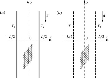
As sketched in figure 1 by employing dimensional quantities, we devise two possible sets of boundary conditions relative to the planes $x=\pm 1/2$ .

Figure 1.

A sketch of (a) Model A and (b) Model B in terms of dimensional quantities.

2.2.1. Model A

We can imagine these planes as isothermal and impermeable following Gill’s approach (Gill Reference Gill1969), namely

(2.5) $$\begin{eqnarray}x=\pm 1/2\!:\quad u=0,T=\pm 1/2.\end{eqnarray}$$

2.2.2. Model B

The alternative is to model the boundaries as permeable. In this case, the external environments in the regions $x<-1/2$ and $x>1/2$ are considered as isothermal fluid reservoirs in a motionless state and kept at different uniform temperatures, $T_{1}$ and $T_{2}$ . In these reservoirs, the pressure distribution is purely hydrostatic, so that the dynamic pressure is zero. Hence, we formulate the boundary conditions

(2.6) $$\begin{eqnarray}x=\pm 1/2\!:\quad p=0,T=\pm 1/2.\end{eqnarray}$$

3.1. Gill’s proof revisited

We obtain the derivative of (3.8a ) with respect to $x$ , obtain $f^{\prime }(x)$ from (3.8b ) and substitute it into the derivative of (3.8a ), so that we can write a single fourth-order differential equation for $h(x)$ , namely

(3.9a ) $$\begin{eqnarray}\displaystyle & h^{\prime \prime \prime \prime }-(2k^{2}+{\it\lambda})h^{\prime \prime }-\text{i}kS(xh^{\prime })^{\prime }+k^{2}(k^{2}+{\it\lambda}+\text{i}kSx)h=0, & \displaystyle\end{eqnarray}$$

(3.9b ) $$\begin{eqnarray}\displaystyle & \left.\begin{array}{@{}lr@{}}x=\pm 1/2\!:\quad h=0,h^{\prime \prime }=0 & \text{Model A},\\ x=\pm 1/2\!:\quad h=0,h^{\prime \prime \prime }=(k^{2}+{\it\lambda}\pm \text{i}kS/2)h^{\prime } & \text{Model B}.\end{array}\right\} & \displaystyle\end{eqnarray}$$

$\bar{h}$

$h$

$-1/2<x<1/2$

$h(\pm 1/2)=0$

(3.10) $$\begin{eqnarray}\displaystyle & & \displaystyle \bar{h}^{\prime }(-1/2)h^{\prime \prime }(-1/2)-\bar{h}^{\prime }(1/2)h^{\prime \prime }(1/2)+\int _{-1/2}^{1/2}|h^{\prime \prime }|^{2}\text{d}x+(2k^{2}+{\it\lambda})\int _{-1/2}^{1/2}|h^{\prime }|^{2}\text{d}x\nonumber\\ \displaystyle & & \displaystyle \quad +\,\text{i}kS\int _{-1/2}^{1/2}x(|h^{\prime }|^{2}+k^{2}|h|^{2})\text{d}x+k^{2}(k^{2}+{\it\lambda})\int _{-1/2}^{1/2}|h|^{2}\text{d}x=0.\end{eqnarray}$$

Since ${\it\lambda}={\it\eta}-\text{i}{\it\omega}$ , the real part of (3.10) gives

(3.11) $$\begin{eqnarray}{\it\gamma}+\int _{-1/2}^{1/2}(|h^{\prime \prime }|^{2}+2k^{2}|h^{\prime }|^{2}+k^{4}|h|^{2})\text{d}x=-{\it\eta}\int _{-1/2}^{1/2}(|h^{\prime }|^{2}+k^{2}|h|^{2})\text{d}x,\end{eqnarray}$$

where

(3.12) $$\begin{eqnarray}{\it\gamma}=\text{Re}[\bar{h}^{\prime }(-1/2)h^{\prime \prime }(-1/2)-\bar{h}^{\prime }(1/2)h^{\prime \prime }(1/2)].\end{eqnarray}$$

If Model A is adopted, then (3.9b ) ensures that ${\it\gamma}=0$ , so that (3.11) allows one to conclude that ${\it\eta}<0$ . This means that the growth rate of normal modes is always negative or, in other words, that the basic flow given by (3.1) is always stable. This conclusion completes the classical Gill’s proof of stability (Gill Reference Gill1969).

The important point is that there is no evidence that Gill’s proof can be extended to Model B. In fact, for Model B, the boundary conditions given by (3.9b ) do not allow one to draw any direct conclusion about ${\it\gamma}$ being negative, zero or positive. Hence, Gill’s method to prove stability becomes ineffective in this case.

3.2. Numerical solution

The lack of a formal proof of stability for Model B leaves open a possibility to investigate the stability or instability of the basic flow, (3.1), through a numerical solution of the eigenvalue problem given by (3.8).

This problem can be solved with a high numerical accuracy by combining the use of an initial value solver for ordinary differential equations and the shooting method. This mathematical technique is well documented in the literature (see, for instance, § 19.1 of the book by Straughan Reference Straughan2004). The procedure can be outlined in two steps:

1. (a) We transform the boundary value problem into an initial value problem by replacing (3.8c ) with

   (3.13a−d ) $$\begin{eqnarray}f(-1/2)=0,\quad f^{\prime }(-1/2)={\it\xi}_{1}+\text{i}{\it\xi}_{2},\quad h(-1/2)=0,\quad h^{\prime }(-1/2)=1.\end{eqnarray}$$
   The last condition, $h^{\prime }(-1/2)=1$ , is meant to fix the otherwise arbitrary scale of the eigenfunctions, while $({\it\xi}_{1},{\it\xi}_{2})$ are unknown real constants to be determined by the shooting method.

   By prescribing the values of $(k,S)$ and trying to guess the values of $({\it\eta},{\it\omega},{\it\xi}_{1},{\it\xi}_{2})$ , the initial value problem given by (3.8a ), (3.8b ) and (3.13) can be solved by an explicit Runge–Kutta algorithm.

2. (b) The shooting method is employed to compute the values of $({\it\eta},{\it\omega},{\it\xi}_{1},{\it\xi}_{2})$ versus the input values $(k,S)$ by satisfying the target conditions given by (3.8c ), namely $f(1/2)=0$ and $h(1/2)=0$ . The eigenfunctions $f$ and $h$ are complex-valued, so that the target conditions yield four real equations.

Both steps can be accomplished by using Mathematica 10 (© Wolfram Research, www.wolfram.com/mathematica), with function NDSolve providing the environment for step (a) and function FindRoot yielding the algorithm to implement step (b).

The most interesting quantity to be computed is ${\it\eta}$ , whose values can be traced, for a fixed $k$ , as $S$ increases starting from 0. In fact, the solution of (3.8) when $S\rightarrow 0$ can be obtained analytically. When $S\rightarrow 0$ , (3.8a ) with the boundary conditions (3.8c ) for Model B admits only the solution $f=0$ , so that $h$ can be determined by solving

(3.14a ) $$\begin{eqnarray}\displaystyle & h^{\prime \prime }-(k^{2}+{\it\eta}-\text{i}{\it\omega})h=0, & \displaystyle\end{eqnarray}$$

(3.14b ) $$\begin{eqnarray}\displaystyle & x=\pm 1/2\!:h=0. & \displaystyle\end{eqnarray}$$

(3.15) $$\begin{eqnarray}h(x)=\frac{1}{n{\rm\pi}}\sin \!\left[n{\rm\pi}\left(x+\frac{1}{2}\right)\right],\quad n=1,2,3,\dots ,\end{eqnarray}$$

with the dispersion relation

(3.16) $$\begin{eqnarray}k^{2}+{\it\eta}-\text{i}{\it\omega}+n^{2}{\rm\pi}^{2}=0,\quad n=1,2,3,\dots .\end{eqnarray}$$

Thus, on recalling that $f=0$ , (3.15) and (3.16) yield

(3.17a−d ) $$\begin{eqnarray}{\it\eta}=-k^{2}-n^{2}{\rm\pi}^{2},\quad {\it\omega}=0,\quad {\it\xi}_{1}=0,\quad {\it\xi}_{2}=0,\quad n=1,2,3,\dots .\end{eqnarray}$$

Equations (3.17) provide the initialisation of the numerical procedure, through steps (a) and (b) described above. With these steps, one evaluates $({\it\eta},{\it\omega},{\it\xi}_{1},{\it\xi}_{2})$ for any given $k$ and gradually increasing values of $S$ starting from $S=0$ .

As expected from (3.17), the values of the growth rate ${\it\eta}$ are initially negative, when $S$ is sufficiently small. The condition ${\it\eta}<0$ means stability. However, if $S$ becomes large enough positive values of ${\it\eta}$ are also found, meaning instability. As $k$ changes, one can draw the geometrical locus of the points where ${\it\eta}=0$ in the parametric plane $(k,S)$ . This locus is the neutral stability curve and it maps the boundary of the instability region.

Table 1.

Validation of the numerical solver: comparison between values of $({\it\eta},{\it\omega},{\it\xi}_{1},{\it\xi}_{2})$ obtained, for $k=1$ and $S=10$ , by an explicit fourth-order Runge–Kutta solver with either fixed step-size, ${\it\delta}x$ , or variable step-size determined adaptively.

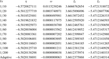
Table 1 reports a validation of the numerical procedure, for $k=1$ and $S=10$ . The assessment of the accuracy is made by comparing the numerical data $({\it\eta},{\it\omega},{\it\xi}_{1},{\it\xi}_{2})$ obtained by using either a fixed step-size specification in the explicit fourth-order Runge–Kutta solver or an adaptive method for variable step-size. The data reported are relative to the branch of normal modes displaying the largest growth rates, ${\it\eta}$ . On decreasing monotonically the value of the step-size ${\it\delta}x$ , table 1 shows that convergence to the data obtained with the adaptive method is attained within at least seven significant figures. The values of ${\it\omega}$ need a specific mention, as the numerical data suggest that ${\it\omega}$ is effectively zero, meaning that the normal mode is non-travelling. All the graphical and numerical results reported in the next section are obtained by the explicit fourth-order Runge–Kutta solver with an adaptive method for variable step-size.

4.1. Linear analysis

In order to establish the possible onset of unstable conditions in the parametric plane $(k,S)$ , we first study the change of the growth rate ${\it\eta}$ versus $S$ for fixed values of $k$ .

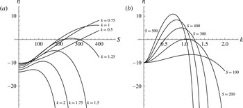
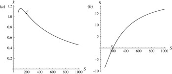
Growth rate plots are reported in figure 2. As for table 1, we examine data relative to the branch with the largest growth rates. Figure 2(a) displays plots of ${\it\eta}$ versus $S$ for fixed values of $k$ , while figure 2(b) shows plots of ${\it\eta}$ versus $k$ for fixed values of $S$ . In figure 2(a), wavenumbers ranging from 0.5 to 2 are considered. Starting from $k=0.5$ , we note that the growth rate ${\it\eta}$ starts from a negative value when $S=0$ (longitudinal rolls), then gradually increases and becomes positive when $S$ is greater than 308.427. The change of sign occurs with a smaller $S$ if $k=0.75$ , and with an even smaller $S$ when $k=1$ . The displayed behaviour is different if we consider $k=1.25$ or larger values of $k$ . In fact, with $k=1.25$ , the growth rate ${\it\eta}$ is initially negative and, as $S$ increases, it becomes positive within the range $222.588<S<299.943$ , then it becomes negative again and starts decreasing. This non-monotonic trend of ${\it\eta}$ versus $S$ is observed also with larger wavenumbers, $k=1.5,1.75,2$ , but the growth rate does not become positive in these cases. A common feature of the data reported in figure 2 is that the value of ${\it\omega}$ is zero, i.e. they are relative to non-travelling modes. We mention that this feature is not general as branches of stable travelling modes ( ${\it\omega}\neq 0$ ) arise outside the range reported in figure 2, where ${\it\eta}$ is lower than $-$ 30. The existence of stable travelling modes had been previously reported by Rees (Reference Rees1988) with reference to Model A boundary conditions. Figure 2(a) suggests the existence of a maximum growth rate ${\it\eta}$ as a function of $S$ for a given $k$ . Likewise, there exists a maximum of function ${\it\eta}(k)$ for a given $S$ (figure 2 b). 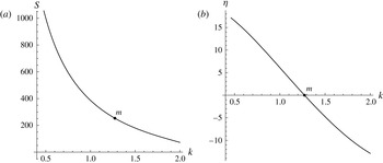The conditions which yield the maximum growth rate ${\it\eta}(S)$ for a fixed $k$ , as well as those for the maximum growth rate ${\it\eta}(k)$ for a fixed $S$ , are reported in figures 3 and 4. Both these figures show the pairs $(k,S)$ , or $(S,k)$ , of maximum growth rate, as well as the maximum growth rate plotted either versus $k$ or versus $S$ . Figures 3 and 4 show also the points, $m$ and $c$ , where the maximum of function ${\it\eta}(S)$ is zero and the maximum of function ${\it\eta}(k)$ is zero, respectively. These figures are useful to detect the fastest growing mode when either the wavenumber is prescribed (figure 3) or the parameter $S$ is prescribed (figure 4). The importance of the fastest growing linear mode in determining the development of convective instability has been recently pointed out by Hewitt, Neufeld & Lister (Reference Hewitt, Neufeld and Lister2013).

Figure 2.

Model B: (a) growth rate ${\it\eta}$ versus $S$ for different wavenumbers $k$ ; (b) growth rate ${\it\eta}$ versus $k$ for different $S$ .

Figure 3.

Model B: line of maximum growth rate, for fixed $k$ , (a) in the plane $(k,S)$ and (b) in the plane $(k,{\it\eta})$ . Point $m$ denotes conditions where the maximum growth rate is zero, namely $k_{m}=1.27291$ and $S_{m}=253.340$ .

Figure 4.

Model B: line of maximum growth rate, for fixed $S$ , (a) in the plane $(S,k)$ and (b) in the plane $(S,{\it\eta})$ . Point $c$ denotes conditions where the maximum growth rate is zero, namely $k_{c}=1.05950$ and $S_{c}=197.081$ .

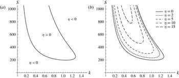
Figure 5(a) shows the neutral stability curve ( ${\it\eta}=0$ ), as well as the stability ( ${\it\eta}<0$ ) and instability ( ${\it\eta}>0$ ) regions in the plane $(k,S)$ . Figure 5(b) shows isolines of ${\it\eta}$ including not only the neutral stability curve ( ${\it\eta}=0$ ), but also some isolines with positive  ${\it\eta}$ .

Figure 5.

Model B: (a) neutral stability curve $S$ versus $k$ and (b) isolines of ${\it\eta}$ with ${\it\eta}\geqslant 0$ in the plane $(k,S)$ .

All neutrally stable modes are non-travelling, viz. ${\it\omega}=0$ . The neutral stability curve has a nose shape, and it displays a minimum at the critical conditions $k=k_{c}$ and $S=S_{c}$ , where

(4.1a,b ) $$\begin{eqnarray}k_{c}=1.05950,\quad S_{c}=197.081.\end{eqnarray}$$

Figure 5 also shows the existence of a maximum value of $k$ bounding the neutrally stable states; this maximum defines the tip of the nose and is placed at

(4.2a,b ) $$\begin{eqnarray}k_{m}=1.27291,\quad S_{m}=253.340.\end{eqnarray}$$

One can immediately realise that the pairs $(k,S)$ defined by (4.1) and (4.2) correspond to the points $c$ and $m$ displayed in figure 4 and figure 3, respectively. No unstable modes could be found when $k>k_{m}$ . Due to the definition of $S$ , given by (3.7), the critical value $S_{c}$ means that instability has its onset with transverse modes ( $k_{y}=k$ ) at a critical Darcy–Rayleigh number $R_{c}=197.081$ . Oblique modes ( $k_{y}<k$ ) are destabilised at higher critical Darcy–Rayleigh numbers, obtained by dividing $S_{c}$ by the ratio $k_{y}/k$ . This yields larger and larger critical values of $R$ as $k_{y}/k$ decreases starting from 1. Eventually, in the limiting case of longitudinal modes ( $k_{y}\rightarrow 0$ ), one obtains $R_{c}\rightarrow \infty$ , which means stability for this type of modes. In other words, Squire’s theorem selecting the two-dimensional transverse modes at onset of instability holds.

An example of a system where the instability defined by the critical conditions (4.1) manifests itself may come from geophysics. Let us consider a gravel layer with thickness $L=2~\text{m}$ and permeability $K=5\times 10^{-10}~\text{m}^{2}$ , saturated with groundwater, ${\it\nu}=10^{-6}~\text{m}^{2}~\text{s}^{-1}$ , ${\it\alpha}=10^{-7}~\text{m}^{2}~\text{s}^{-1}$ and ${\it\beta}=2\times 10^{-4}~\text{K}^{-1}$ . Instability, $R>R_{c}$ , occurs when the temperature difference across the layer is larger than 10 K.

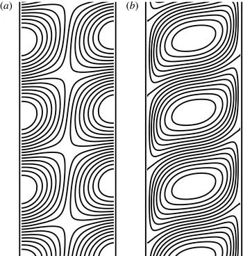
A sketch of the streamlines and isotherms for the secondary flow arising at onset of convection with $k_{c}=1.05950$ and $R_{c}=197.081$ is shown in figure 6. Due to the expression of normal modes, (3.5), the convection pattern forms a periodic sequence of alternate clockwise and counterclockwise cells, so that arrows are not strictly needed in order to understand the orientation of streamlines in figure 6. As discussed above, this secondary flow is through non-travelling transverse modes. One may see that the streamlines are cut by the boundaries, so that the secondary flow penetrates both the left external environment ( $x<-1/2$ ) and the right external environment ( $x>1/2$ ). Thus, one may question the reliability of Model B at supercritical conditions, where the growing disturbances achieve finite or large amplitudes. At supercritical conditions, imagining the external environments as quiescent reservoirs at uniform temperature and hydrostatic pressure distribution may be a poor model. In fact, the penetrating secondary flow is likely to induce inhomogeneities of the temperature and dynamic pressure distributions therein.

Figure 6.

Model B: (a) streamlines and (b) isotherms of the secondary flow induced by transverse modes at onset of instability with the critical values $(k_{c},S_{c})$ , (4.1).

4.2. A few examples of the nonlinear regime

When the flow conditions are supercritical, i.e. $R>R_{c}$ , a nonlinear analysis is needed to trace the time evolution of finite-amplitude perturbations. This means that the full nonlinear governing equations (2.1) and (2.6) have to be solved. The solution can be sought numerically by employing a finite element method. An efficient tool for achieving this solution is COMSOL Multiphysics (© COMSOL Inc., www.comsol.com/comsol-multiphysics). The solution can be carried out with reference to transverse modes, so that the computational domain is two-dimensional. The domain defined for the solver is a rectangle in the $(x,y)$ -plane with $-1/2\leqslant x\leqslant 1/2$ and $-{\rm\Delta}y/2\leqslant y\leqslant {\rm\Delta}y/2$ . In the solution of the full nonlinear equations, the role of normal modes is different from that in the linear analysis. In fact, the nonlinear time evolution of a normal mode with wavenumber $k$ , prescribed at time $t=0$ , implies its mixing with all possible normal modes. Another aspect of the nonlinear evolution of unstable perturbations is the phenomenon of saturation. Saturation means that the initially exponential time-growth of the perturbation is damped, so that the growth rate decreases and it may even tend to 0 as $t\rightarrow \infty$ . In this case, the unbounded exponential growth predicted by the linear stability analysis is drastically modified in the nonlinear domain, thus leading to the prediction of asymptotic stationary states, different from the basic state, approached at large times. The phenomenon of saturation may also lead to the conclusion that the effects of instability are not always as remarkable as one would infer from the linear stability analysis. Before discussing a few sample cases in the supercritical regime, it is worth describing some details of the numerical solution. Periodicity conditions for pressure and temperature are prescribed at the end boundaries, $y=-{\rm\Delta}y/2$ and $y={\rm\Delta}y/2$ . An unstructured uniform mesh with triangular elements is defined in the computational domain. Two cases are studied, with ${\rm\Delta}y=4{\rm\pi}$ and ${\rm\Delta}y=8{\rm\pi}$ . With ${\rm\Delta}y=4{\rm\pi}$ the number of triangular elements is 12 630, while for ${\rm\Delta}y=8{\rm\pi}$ the number of elements is 25 184. The mesh refinement has been chosen so that the numerical results are mesh-independent within graphical resolution. In the four sample cases analysed, the time evolution tends to a stationary state different from the basic state.

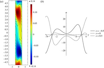
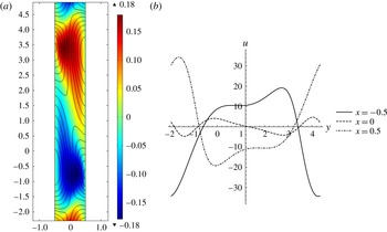
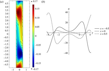
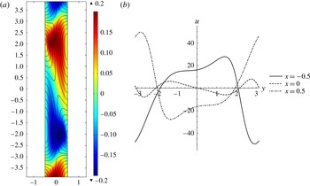
The four cases illustrated in figures 7–10 relate to $R=400$ and $R=500$ and, for each fixed value of $R$ , they describe different patterns along the vertical $y$ direction. In fact, we assigned different values of ${\rm\Delta}y$ , namely ${\rm\Delta}y=8{\rm\pi}$ and ${\rm\Delta}y=4{\rm\pi}$ , to explore different periods of the cellular patterns. The region plotted in figures 7(a)–10(a) is not the whole range of $y$ , but approximately one period. In these frames, the colour map of the temperature perturbation, viz. the difference between the temperature and the temperature in the basic state, is plotted together with the streamlines of the perturbation velocity, namely the excess velocity with respect to the basic state. Figures 7(b)–10(b) display the horizontal velocity component, $u$ , as a function of $y$ for $x=-1/2,0,1/2$ . We recall that $u=0$ in the basic state, so that this velocity component arises from the perturbation of the basic state. In the four cases examined, the streamlines show a natural mass discharge/recharge to/from the external environments. Like the phenomenon reported in the paper by Elder (Reference Elder1967), the lateral mass flux is not a very intense effect, both for $R=400$ and for $R=500$ . In fact, the maximum values of $u$ at the lateral boundaries are slightly greater than 20 (figure 7) or 30 (figure 8), when $R=400$ , and around 40 (figure 9) or slightly greater (figure 10), when $R=500$ . A reference value to estimate these maximum values of $u$ is the maximum vertical velocity in the basic state, that is $R/2$ . This is 200, for figures 7 and 8, and 250, for figures 9 and 10. The temperature perturbation is comparable with the basic state temperature, as the maxima in the colour maps are not much less than half the maximum temperature in the basic state, namely $T=1/2$ .

Figure 7.

Asymptotic steady state for $t\rightarrow \infty$ in the nonlinear regime with $R=400$ and ${\rm\Delta}y=8{\rm\pi}$ : (a) colour map over one period of the temperature perturbation with superposed streamlines of the velocity perturbation in the $(x,y)$ -plane; (b) plot over one period of the horizontal velocity component $u$ as a function of $y$ at different fixed values of $x$ .

Figure 8.

Asymptotic steady state for $t\rightarrow \infty$ in the nonlinear regime with $R=400$ and ${\rm\Delta}y=4{\rm\pi}$ : (a) colour map over one period of the temperature perturbation with superposed streamlines of the velocity perturbation in the $(x,y)$ -plane; (b) plot over one period of the horizontal velocity component $u$ as a function of $y$ at different fixed values of $x$ .

A final remark concerns the periodicity of the patterns as related to the prescribed values of ${\rm\Delta}y$ . One may notice that, when ${\rm\Delta}y=8{\rm\pi}$ (figures 7 and 9), three periods are allowed over the height of the computational domain. On the other hand, when ${\rm\Delta}y=4{\rm\pi}$ (figures 8 and 10), two periods are allowed. With reference to the case $R=400$ , there is a simple physical argument justifying this pattern selection. In fact, over a height of $8{\rm\pi}$ with periodic end conditions, allowed normal modes are such that $k=n/4$ , where $n=1,2,3,\dots .$ Over a height of $4{\rm\pi}$ , allowed normal modes are with $k=n/2$ . Figure 2(b) reveals that, with $R=400$ , the linear mode of type $k=n/4$ with the largest growth rate is for $n=3$ , while the fastest growing mode with $k=n/2$ is for $n=2$ . This explains why the three-period pattern is preferred for a height of $8{\rm\pi}$ , while the two-period pattern is preferred for a height of $4{\rm\pi}$ . On the other hand, this reasoning does not work properly when $R=500$ . In fact, by employing the data reported in figure 2(b), the linear mode of type $k=n/4$ with the largest growth rate is again for $n=3$ , but the fastest growing mode with $k=n/2$ is for $n=1$ . Therefore, one should expect that a one-period pattern is selected when the height is $4{\rm\pi}$ , unlike what is found by the nonlinear analysis. An explanation of the ineffectiveness of the fastest growing linear mode in determining the periodicity of the actual nonlinear pattern is related to the highly supercritical regime taking place at $R=500$ . In this regime, the nonlinear dynamics prevails so that the fastest growing linear mode is unable to drive the pattern selection mechanism.

Figure 9.

Asymptotic steady state for $t\rightarrow \infty$ in the nonlinear regime with $R=500$ and ${\rm\Delta}y=8{\rm\pi}$ : (a) colour map over one period of the temperature perturbation with superposed streamlines of the velocity perturbation in the $(x,y)$ -plane; (b) plot over one period of the horizontal velocity component $u$ as a function of $y$ at different fixed values of $x$ .

Figure 10.

Asymptotic steady state for $t\rightarrow \infty$ in the nonlinear regime with $R=500$ and ${\rm\Delta}y=4{\rm\pi}$ : (a) colour map over one period of the temperature perturbation with superposed streamlines of the velocity perturbation in the $(x,y)$ -plane; (b) plot over one period of the horizontal velocity component $u$ as a function of $y$ at different fixed values of $x$ .

The nonlinear analysis in the supercritical regime carried out so far has definitely no aim of generality. There is much more work to do for an exhaustive investigation of this regime. An open question is, for instance, the multiplicity of periodic cellular structures that are allowed in the asymptotic steady states approached when $t\rightarrow \infty$ . In this regard, the role of the end conditions set at the extrema of the $y$ -range needs further investigation. In particular, an interesting point is the description of what may happen if the periodic end conditions, at $y=-{\rm\Delta}y/2$ and $y={\rm\Delta}y/2$ , are replaced by impermeability and thermal insulation conditions. This alternative may be appropriate in order to model a vertical slab with a finite height.