



%20--%3e%3c!DOCTYPE%20svg%20PUBLIC%20'-//W3C//DTD%20SVG%201.0//EN'%20'http://www.w3.org/TR/2001/REC-SVG-20010904/DTD/svg10.dtd'%3e%3csvg%20version='1.0'%20id='Layer_1'%20xmlns='http://www.w3.org/2000/svg'%20xmlns:xlink='http://www.w3.org/1999/xlink'%20x='0px'%20y='0px'%20width='64px'%20height='64px'%20viewBox='5.5%20-3.5%2064%2064'%20enable-background='new%205.5%20-3.5%2064%2064'%20xml:space='preserve'%3e%3cg%3e%3ccircle%20fill='%23FFFFFF'%20fill-opacity='0'%20cx='37.785'%20cy='28.501'%20r='28.836'/%3e%3cpath%20fill='%23595959'%20d='M37.441-3.5c8.951,0,16.572,3.125,22.857,9.372c3.008,3.009,5.295,6.448,6.857,10.314%20c1.561,3.867,2.344,7.971,2.344,12.314c0,4.381-0.773,8.486-2.314,12.313c-1.543,3.828-3.82,7.21-6.828,10.143%20c-3.123,3.085-6.666,5.448-10.629,7.086c-3.961,1.638-8.057,2.457-12.285,2.457s-8.276-0.808-12.143-2.429%20c-3.866-1.618-7.333-3.961-10.4-7.027c-3.067-3.066-5.4-6.524-7-10.372S5.5,32.767,5.5,28.5c0-4.229,0.809-8.295,2.428-12.2%20c1.619-3.905,3.972-7.4,7.057-10.486C21.08-0.394,28.565-3.5,37.441-3.5z%20M37.557,2.272c-7.314,0-13.467,2.553-18.458,7.657%20c-2.515,2.553-4.448,5.419-5.8,8.6c-1.354,3.181-2.029,6.505-2.029,9.972c0,3.429,0.675,6.734,2.029,9.913%20c1.353,3.183,3.285,6.021,5.8,8.516c2.514,2.496,5.351,4.399,8.515,5.715c3.161,1.314,6.476,1.971,9.943,1.971%20c3.428,0,6.75-0.665,9.973-1.999c3.219-1.335,6.121-3.257,8.713-5.771c4.99-4.876,7.484-10.99,7.484-18.344%20c0-3.543-0.648-6.895-1.943-10.057c-1.293-3.162-3.18-5.98-5.654-8.458C50.984,4.844,44.795,2.272,37.557,2.272z%20M37.156,23.187%20l-4.287,2.229c-0.458-0.951-1.019-1.619-1.685-2c-0.667-0.38-1.286-0.571-1.858-0.571c-2.856,0-4.286,1.885-4.286,5.657%20c0,1.714,0.362,3.084,1.085,4.113c0.724,1.029,1.791,1.544,3.201,1.544c1.867,0,3.181-0.915,3.944-2.743l3.942,2%20c-0.838,1.563-2,2.791-3.486,3.686c-1.484,0.896-3.123,1.343-4.914,1.343c-2.857,0-5.163-0.875-6.915-2.629%20c-1.752-1.752-2.628-4.19-2.628-7.313c0-3.048,0.886-5.466,2.657-7.257c1.771-1.79,4.009-2.686,6.715-2.686%20C32.604,18.558,35.441,20.101,37.156,23.187z%20M55.613,23.187l-4.229,2.229c-0.457-0.951-1.02-1.619-1.686-2%20c-0.668-0.38-1.307-0.571-1.914-0.571c-2.857,0-4.287,1.885-4.287,5.657c0,1.714,0.363,3.084,1.086,4.113%20c0.723,1.029,1.789,1.544,3.201,1.544c1.865,0,3.18-0.915,3.941-2.743l4,2c-0.875,1.563-2.057,2.791-3.541,3.686%20c-1.486,0.896-3.105,1.343-4.857,1.343c-2.896,0-5.209-0.875-6.941-2.629c-1.736-1.752-2.602-4.19-2.602-7.313%20c0-3.048,0.885-5.466,2.658-7.257c1.77-1.79,4.008-2.686,6.713-2.686C51.117,18.558,53.938,20.101,55.613,23.187z'/%3e%3c/g%3e%3c/svg%3e)
%20--%3e%3c!DOCTYPE%20svg%20PUBLIC%20'-//W3C//DTD%20SVG%201.0//EN'%20'http://www.w3.org/TR/2001/REC-SVG-20010904/DTD/svg10.dtd'%3e%3csvg%20version='1.0'%20id='Layer_1'%20xmlns='http://www.w3.org/2000/svg'%20xmlns:xlink='http://www.w3.org/1999/xlink'%20x='0px'%20y='0px'%20width='64px'%20height='64px'%20viewBox='5.5%20-3.5%2064%2064'%20enable-background='new%205.5%20-3.5%2064%2064'%20xml:space='preserve'%3e%3cg%3e%3ccircle%20fill='%23FFFFFF'%20fill-opacity='0'%20cx='37.637'%20cy='28.806'%20r='28.276'/%3e%3cg%3e%3cpath%20fill='%23595959'%20d='M37.443-3.5c8.988,0,16.57,3.085,22.742,9.257C66.393,11.967,69.5,19.548,69.5,28.5c0,8.991-3.049,16.476-9.145,22.456%20C53.879,57.319,46.242,60.5,37.443,60.5c-8.649,0-16.153-3.144-22.514-9.43C8.644,44.784,5.5,37.262,5.5,28.5%20c0-8.761,3.144-16.342,9.429-22.742C21.101-0.415,28.604-3.5,37.443-3.5z%20M37.557,2.272c-7.276,0-13.428,2.553-18.457,7.657%20c-5.22,5.334-7.829,11.525-7.829,18.572c0,7.086,2.59,13.22,7.77,18.398c5.181,5.182,11.352,7.771,18.514,7.771%20c7.123,0,13.334-2.607,18.629-7.828c5.029-4.838,7.543-10.952,7.543-18.343c0-7.276-2.553-13.465-7.656-18.571%20C50.967,4.824,44.795,2.272,37.557,2.272z%20M46.129,20.557v13.085h-3.656v15.542h-9.944V33.643h-3.656V20.557%20c0-0.572,0.2-1.057,0.599-1.457c0.401-0.399,0.887-0.6,1.457-0.6h13.144c0.533,0,1.01,0.2,1.428,0.6%20C45.918,19.5,46.129,19.986,46.129,20.557z%20M33.042,12.329c0-3.008,1.485-4.514,4.458-4.514s4.457,1.504,4.457,4.514%20c0,2.971-1.486,4.457-4.457,4.457S33.042,15.3,33.042,12.329z'/%3e%3c/g%3e%3c/g%3e%3c/svg%3e)
1. Introduction
The study of multiphase flows is often limited by the computational effort involved in solving the Navier–Stokes (NS) equations (Glasser, Kevrekidis & Sundaresan Reference Glasser, Kevrekidis and Sundaresan1997). One such example, the flow of thin films of liquid on inclined planes, has fascinated researchers not only because of the wide range of industrial applications but also because of the interesting dynamics of the liquid–air interface (Kalliadasis et al. Reference Kalliadasis, Ruyer-Quil, Scheid and Velarde2012). The NS equations accurately describe the fluid motion and also the evolution of the surface but suffer from a high computational cost (Pettas et al. Reference Pettas, Karapetsas, Dimakopoulos and Tsamopoulos2019a,Reference Pettas, Karapetsas, Dimakopoulos and Tsamopoulosb). To this end, significant effort has led to several approximate interface evolution equations that are much simpler to solve but are nevertheless valid under specific assumptions and limitations. Beyond their limits of validity, it is often found that they yield non-physical solutions, or even blow up (Kalliadasis et al. Reference Kalliadasis, Ruyer-Quil, Scheid and Velarde2012), posing significant restrictions to their applicability. In more recent studies, weighted integral boundary layer models are found to compare favourably to NS simulations for moderate Reynolds numbers and even three-dimensional flows (Dietze et al. Reference Dietze, Rohlfs, Nährich, Kneer and Scheid2014). These surrogate models are very economical and are included even in open source codes (Rohlfs, Rietz & Scheid Reference Rohlfs, Rietz and Scheid2018), showing remarkable accuracy even in flow regimes exhibiting highly nonlinear waves (Chakraborty et al. Reference Chakraborty, Nguyen, Ruyer-Quil and Bontozoglou2014). Alternatives to models that solve partial differential equations (PDEs) are also available that compute the film height by numerical integration based on the aggregation of droplets (Bharadwaj et al. Reference Bharadwaj, Kuhnert, Bordas and Suchde2022).
The evolution of successful surrogate models has taken place over the past decades and relies on significant subject matter expertise to form meaningful assumptions and involved algebra. Our goal here is to develop novel, robust and efficient data-driven/data-assisted models, not restricted to applications of thin film flow, that combine physical and mathematical insight with machine learning strategies, in order to drastically enable computational fluid dynamics and break new barriers in flow control, uncertainty quantification and shape optimization.
The implementation of data-driven methods is gaining popularity in diverse fluid-related applications. Recently, nonlinear manifold learning and specifically isomap (Balasubramanian & Schwartz Reference Balasubramanian and Schwartz2002) was implemented to derive a low-dimensional description of an ensemble of flow field snapshots as an alternative to proper orthogonal decomposition (POD), ultimately aiming at developing an economical surrogate (Farzamnik et al. Reference Farzamnik, Ianiro, Discetti, Deng, Oberleithner, Noack and Guerrero2023). Deep learning has been proposed in order to produce closures of large-eddy simulations (LES) and Reynolds-averaged NS models, by adding neural network-derived terms into the governing equations (Sirignano & MacArt Reference Sirignano and MacArt2023). Data-driven viscous damping terms have been estimated for sloshing a rectangular tank (Miliaiev & Timokha Reference Miliaiev and Timokha2023), where machine learning is implemented in conjunction with an appropriately formulated loss function that relies on experimental measurements. Machine learning is implemented to derive multifidelity models (Rezaeiravesh, Mukha & Schlatter Reference Rezaeiravesh, Mukha and Schlatter2023), and an ensemble of neural networks is applied to develop a wall model for LES based on the assumption that the flow can be thought of as a combination of blocks (Lozano-Durán & Bae Reference Lozano-Durán and Bae2023). Flow control is also a popular field where machine learning is implemented (Sonoda et al. Reference Sonoda, Liu, Itoh and Hasegawa2023; Zhang, Fan & Zhou Reference Zhang, Fan and Zhou2023). Recently, artificial neural network–based nonlinear algebraic models were presented for the LES of compressible wall-bounded turbulence (Xu et al. Reference Xu, Wang, Yu and Chen2023). A model based on a convolutional neural network is proposed so as to reconstruct the three-dimensional turbulent flows beneath a free surface using surface measurements, including the surface elevation and surface velocity (Xuan & Shen Reference Xuan and Shen2023). Also, data-driven modelling has recently been proposed in the context of unsteady wall pressure fields (Meloni et al. Reference Meloni, Centracchio, de Paola, Camussi and Iemma2023).
This work presents a methodology for deriving data-driven PDEs for the film amplitude, based on a collection of NS simulation data that are not subject to restrictions and assumptions for the flow and, hence, are more general. Our work falls in the category of dynamical system identification (Rico-Martínez et al. Reference Rico-Martínez, Krischer, Kevrekidis, Kube and Hudson1992; Krischer et al. Reference Krischer, Rico-Martínez, Kevrekidis, Rotermund, Ertl and Hudson1993; González-García, Rico-Martínez & Kevrekidis Reference González-García, Rico-Martínez and Kevrekidis1998; Kemeth et al. Reference Kemeth, Bertalan, Thiem, Dietrich, Moon, Laing and Kevrekidis2022). Recently increased interest in PDE identification has led to the development of alternative algorithmic tools, such as sparse identification of nonlinear dynamical systems using dictionaries (Brunton, Proctor & Kutz Reference Brunton, Proctor and Kutz2016; Rudy et al. Reference Rudy, Brunton, Proctor and Kutz2017), PDE-net (Long et al. Reference Long, Lu, Ma and Dong2018), physics-informed neural networks (Raissi, Perdikaris & Karniadakis Reference Raissi, Perdikaris and Karniadakis2019) and others (Chen et al. Reference Chen, Rubanova, Bettencourt and Duvenaud2018; Vlachas et al. Reference Vlachas, Byeon, Wan, Sapsis and Koumoutsakos2018, Reference Vlachas, Arampatzis, Uhler and Koumoutsakos2022). Our algorithmic approach can be implemented on data from detailed PDE simulations (Psarellis et al. Reference Psarellis, Lee, Bhattacharjee, Datta, Bello-Rivas and Kevrekidis2022), agent-based modelling (Arbabi & Kevrekidis Reference Arbabi and Kevrekidis2021; Lee et al. Reference Lee, Psarellis, Siettos and Kevrekidis2022) or lattice Boltzmann simulations (Lee et al. Reference Lee, Kooshkbaghi, Spiliotis, Siettos and Kevrekidis2020; Galaris et al. Reference Galaris, Fabiani, Gallos, Kevrekidis and Siettos2022), among others. Extensions of PDE identification including grey box or closure identification (such as those explored in our work) have been studied in the context of various applications (Parish & Duraisamy Reference Parish and Duraisamy2016; Pan & Duraisamy Reference Pan and Duraisamy2018; Duraisamy, Iaccarino & Xiao Reference Duraisamy, Iaccarino and Xiao2019; Lee et al. Reference Lee, Dietrich, Karniadakis and Kevrekidis2019; Lee et al. Reference Lee, Psarellis, Siettos and Kevrekidis2022; Psarellis et al. Reference Psarellis, Lee, Bhattacharjee, Datta, Bello-Rivas and Kevrekidis2022; Kemeth et al. Reference Kemeth, Alonso, Echebarria, Moldenhawer, Beta and Kevrekidis2023). In the relevant literature, the Kuramoto–Sivashinsky (KS) equation, selected in this work as a low-fidelity counterpart of the NS equations, has served as a benchmark case study, due to its wealth of dynamic responses and highly nonlinear nature (González-García et al. Reference González-García, Rico-Martínez and Kevrekidis1998; Raissi & Karniadakis Reference Raissi and Karniadakis2017; Vlachas et al. Reference Vlachas, Byeon, Wan, Sapsis and Koumoutsakos2018; Floryan & Graham Reference Floryan and Graham2022; Linot et al. Reference Linot, Burby, Tang, Balaprakash, Graham and Maulik2023).
The results of the learned PDE are compared with the ground-truth NS results and also the results of the KS equation. It is expected that past a certain limit, the KS equation will perform poorly and produce non-physical solutions. Yet it is still useful in the context of learning an accurate amplitude PDE, as will be shown, in two different ways. In the first ‘grey box’ model approach, an additive correction of the KS equation can be learned from NS data as a sort of calibration of the low-fidelity model against high-fidelity data. In this context, the data-driven model provides a measure of the discrepancy between the approximate equation and the ground truth, and serves to inform as to the actual limits of applicability of the KS equation in terms of the flow parameter, here the Reynolds number. In the second approach, which we call the ‘functional correction grey box model’, certain observations of the KS formula, such as the value of its right-hand side, its derivatives or even values in specific nearby time instances or nearby points in space, are used as inputs to the learned model.
In addition, reduced representations of the NS data, including full velocity fields and fluid film height, are further exploited for out-of-sample predictions from partial data at the small data limit. Nonlinear manifold learning, specifically diffusion maps (DMAPs) and linear methods, i.e. POD, are initially implemented in order to derive a low-order description of the high-dimensional dataset. It is then shown that efficient interpolation in the reduced space can help recover entire sets of data from partial information. Specifically, it will be demonstrated that full velocity profiles, parameter values and film height measurements can be predicted given a handful of values for the film height at specific locations. The advantages of ‘gappy’ diffusion maps over its linear counterpart, gappy POD, are discussed in relation to the parsimony of the description of the manifold that contains the data and to the location of the known measurements.
2. Governing equations: ground truth and surrogate model
The flow of a liquid film on an inclined plane (see figure 1) is described, in two dimensions, by conservation equations for mass and momentum, written in dimensionless form as
 \begin{equation} \left.\begin{array}{c} \boldsymbol{\nabla} \boldsymbol{\cdot} \boldsymbol{u} = 0, \\ R \dfrac{\partial \boldsymbol{u}}{\partial t}={-} R (\boldsymbol{u} \boldsymbol{\cdot} \boldsymbol{\nabla} \boldsymbol{u}) - \boldsymbol{\nabla} P + \nabla^2\boldsymbol{u} + F \boldsymbol{g}, \end{array}\right\} \end{equation}
where  $\boldsymbol {u}=( u_x, u_y)^\textrm {T}$ and
 $P$ are the dimensionless velocity vector and pressure, respectively, and
 $\boldsymbol {\nabla }=( \partial _x, \partial _y )$ denotes the gradient operator for Cartesian coordinates. We also define the unit gravity vector
 $\boldsymbol {g}=(\sin \theta,-\cos \theta )^\textrm {T}$. Using the characteristic Nusselt scales for the velocity vector and all lengths,
 \begin{equation} U_N=\left(\frac{Q^{2} \rho g \sin(\theta)}{3\mu}\right)^{1/3},\quad H_N=\left(\frac{3\mu Q}{ \rho g \sin(\theta)}\right)^{1/3}, \end{equation}
the dimensionless groups that emerge are the Reynolds number  $R$, the Weber number
 $W$ and the Stokes number
 $F$, defined as
 \begin{equation} R = \frac{\rho Q}{\mu}, \quad W = \frac{\sigma}{\rho g H_N^2}, \quad F = \frac{3}{\sin \theta}. \end{equation}
Here,  $\rho$,
 $\mu$ and
 $\sigma$ are the liquid density, the viscosity and the liquid–air surface tension, respectively, while
 $Q$ denotes the volumetric flow rate per unit length normal to the cross-section.
Cross-section of a film flowing on a plane, inclined with respect to the horizontal by angle  $\theta$. Here
 $H=1$ is the dimensionless Nusselt film height.

Along the liquid–air interface, a normal stress balance between capillary force and viscous stress is applied,
 \begin{equation} \boldsymbol{n}\boldsymbol{\cdot} \boldsymbol{T} = W F \kappa \boldsymbol{n}. \end{equation}
Here, the total stress tensor is defined as  $\boldsymbol {T}=-P\boldsymbol {I}+(\boldsymbol {\nabla } \boldsymbol {u}+(\boldsymbol {\nabla }\boldsymbol {u})^\textrm {T})$,
 $\boldsymbol {n}$ is the unit vector normal to the interface, outward with respect to the film. Note that in (2.4) the ambient pressure has been set equal to zero (datum pressure) without loss of generality. The mean curvature is
 $\kappa =-\nabla _s \boldsymbol {\cdot } \boldsymbol {n}$ , with
 $\nabla _s=(\boldsymbol {I}-\boldsymbol {nn})\boldsymbol {\cdot } \boldsymbol {\nabla }$. The rest of the boundary conditions include the no-slip condition at the liquid–solid plane interface (denoted as AB in figure 1) and periodic boundary conditions at the lateral domain boundaries (AD and BC in figure 1).
The kinematic boundary condition, which specifies that the velocity of the interface that is normal to the boundary is equal to the velocity of the fluid that is normal to the boundary, ensuring no mass transfer through the interface, completes the set of governing equations
 \begin{equation} \boldsymbol{n}\boldsymbol{\cdot} (h_t \boldsymbol{e}_y)=\boldsymbol{n}\boldsymbol{\cdot} \boldsymbol{u}. \end{equation}
The NS data, which consist our ground truth, are derived by solving the time-dependent equations in an Eulerian frame, discretized with the finite element method, using COMSOL Multiphysics®. We consider the flow over a vertical plane, schematically presented in figure 1, i.e.  $\theta =90^\circ$ with a domain of dimensionless length,
 $l=L/H_N=95$;
 $L$ denotes the dimensional length of the domain. The value of the Weber number used in the simulations is
 $W=278$. We start our simulations from an initial condition corresponding to a flat film perturbed by a sinusoidal perturbation with amplitude
 $\sim$3 % of the dimensionless Nusselt film height,
 $H=1$. The height of the film,
 $h(x,t)$, is collected at each time step until a steady travelling wave is formed.
2.1. Surrogate model – the KS equation
The single-equation surrogate of the amplitude, selected in this study, is the KS equation. Assuming the flow over a vertical plane, the KS equation can be written as
 \begin{equation} \left.\begin{array}{c} \phi_\tau={-}\alpha(\phi \phi_\xi+\phi_{\xi\xi})-4\phi_{\xi\xi\xi\xi} \quad \textrm{for}\ \xi\in[0,2\pi], \\ \alpha=\dfrac{8}{5} \dfrac{R F}{\epsilon^2 W}. \end{array}\right\} \end{equation}
The detailed derivation of the KS equation from NS equations can be found in Shlang & Sivashinsky (Reference Shlang and Sivashinsky1982), Chang (Reference Chang1986) and Brown (Reference Brown1992) and it is summed up here for completeness. It is based on the following assumptions.
(i) The film is thin,
 $\epsilon =2 \pi H_N/L \ll 1$.
(ii) The waves are long,
${\partial h}/{\partial x} \ll 1$.(iii) The mean height of the film is much larger than the deviation from the mean.


Under these assumptions, it is possible to exploit the small parameter  $\epsilon$ and employ a perturbation expansion for all dependent variables, i.e. velocities, pressure and interfacial height; e.g. the interfacial height is given by
 $h\approx 1+\epsilon \eta + O(\epsilon ^2)$, where
 $\eta$ denotes the deviation from the mean film height. Restricting to the case of laminar flow with
 $R=O(1)$,
 $F=O(1)$ and
 $W=O(\epsilon ^{-2})$ and neglecting higher-order terms, the kinematic condition (written in terms of the deviation,
 $\eta$) may be reduced to
 $\eta _t+F\eta _x=0$, indicating that waves travel with speed
 $F$. Taking this into account, a new variable
 $\xi =\epsilon (x-Ft)$ can be introduced to obtain constant shape waves travelling with speed
 $F$. Moreover, the amplitude is rescaled according to
 $\phi =({15}/{RF})\eta$. Finally, since it is known that the wave amplitude varies on a slow time scale compared with the travelling motion, a change in the time variable is introduced, i.e.
 $\tau = ({\epsilon ^4 W F}/{12}) t$. In the end, the KS equation (2.6) is obtained as a function of the new defined variables.
2.2. The NS vs KS equation: bifurcation diagram
The KS equation will be used extensively in the discussion that will follow mostly in terms of the derivation of variations of the data-driven model. Therefore, it would be useful to briefly discuss the limitations of the KS equation before proceeding with the presentation of our results. Even though it is well known that the KS equation is valid for Reynolds number values of O(1), to the best of our knowledge, there is no direct comparison in the literature of the KS equation to the NS equation results. To clearly present the limitations of the KS equation, here we plot in figure 2 the norm of the amplitude distribution,  $\|\eta \|$, with respect to both the Reynolds number and the KS parameter
 $\alpha$.
Bifurcation diagram of the NS and KS equations.

Both equations predict very similar results for  $1\leq R \leq 3.4$ (or
 $4\leq \alpha \leq 13.43$). In this range of parameter values the solution of the KS equation is a stationary wave (in a co-moving frame with speed
 $c=3$), whereas the NS equation, solved in an Eulerian frame evolves into a travelling wave with a steady and unchanged shape and speed
 $c=3$. Past that point (
 $R=3.4$ and
 $\alpha =13.43$), the speed of the wave becomes larger than 3 and, hence, the solution of the KS equation is also travelling (with speed
 $c-3$). Up to approximately
 $R=4.3$ (
 $\alpha =16.5$) the KS solution gradually deviates from the NS solution. For higher values of
 $\alpha$, i.e.
 $\alpha >16.998$, the solution of the KS equation is a so-called ‘pulsing’ wave, as described in detail in Kevrekidis, Nicolaenko & Scovel (Reference Kevrekidis, Nicolaenko and Scovel1990). The pulsing waves oscillate between two waveforms that are
 $\pi$ periodic in space and are
 $\pi /2$ shifts of each other. Such a solution has not been reported for the NS equations.
3. Physics-agnostic and physics-infused data-driven models
3.1. Black box model: learning the PDE
Here the goal is to use data from the NS simulations to learn a PDE of the general form
 \begin{equation} \frac{\partial{\eta}}{\partial t}=f(\eta,\eta_x,\eta_{xx},\eta_{xxx},\eta_{xxxx},R). \end{equation}
The function  $f$ is approximated by a feed forward neural network with two hidden layers with 15 neurons and a tanh activation function, implemented in Tensorflow (Abadi et al. Reference Abadi2015). The mean squared error is used as a loss function along with the Adam optimizer. The inputs to the neural network are the amplitude and four spatial derivatives of the amplitude, along with the
 $R$ value, as extracted from the NS simulations. Specifically, the NS model is implemented for 20 parameter values, and snapshots, i.e. time instances of the film surface evolution are collected in equally sized time steps (
 $dt=1$ is the dimensionless time unit). The spatial derivatives, up to fourth order are computed using Fourier transforms, in each point in space and time. The output of the neural network is the time derivative of the amplitude, which can be extracted directly from the NS code (although it can also be easily computed, e.g. with finite differences).
In total, 75 000 data points (pairs of local values of the inputs and output) per parameter value are used to train the neural network and once this is done, the right-hand side of the PDE in (3.1) can be used in conjunction with any method of integration in time, such as the Runge–Kutta method. The attractors that correspond to a steady travelling wave that resulted from the integration of the learned PDE are shown in figure 3 for a representative selection of parameter values. The attractor of the neural network-derived PDE, shown in black, is almost a perfect match with the ground-truth results of the NS (dashed line).
‘Black box’ model performance. Attractors for different  $R$ numbers derived by (i) the NS equation (dashed line), (ii) the KS equation (grey) and (iii) the NN-derived PDE (black); all results are rescaled in the NS scaling. (a)
 $R = 1.45$, (b)
 $R = 1.95$, (c)
 $R = 3.30$, (d)
 $R = 3.70$, (e)
 $R = 4.20$ and (f)
 $R = 5.20$.

For reference and comparison, the KS results (appropriately rescaled according to the scaling factors detailed in Appendix A) are shown in the same plot (grey line). The KS equation performs well for small values of the  $R$ number (
 $R<3.3$), but then progressively start to deviate quantitatively for increasing values of
 $R$. This is shown in figure 4, where a snapshot of the amplitude derived by the KS equation, the NS equations and the ‘black box’ model are shown alongside the corresponding phase portraits for
 $R=1.95$ and
 $R=4.2$. This figure also shows the error along time integration, which illustrates the fact that, on average, the small numerical error remains constant. These two
 $R$ values are chosen to demonstrate that the black box model outperforms the KS equation even in parameter values where the latter is inaccurate (
 $R=4.2$). Despite the apparent failure of the KS equation to capture the wave dynamics accurately, it still yields qualitatively good results.
Black box model wave comparison. (a,d) Attractors; (b,e) time instance of the amplitude, derived by the NS equation (dashed line), the KS equation (grey line) and the NN-derived PDE (black line); (c,f) error. Results are shown for (a–c)  $R=1.95$, (d–f)
 $R=4.2$; all results are rescaled in the NS scaling.

It is important to note here that the black box model methodology yields accurate data-driven models, also in different flow regimes such as in the case of solitary waves, appearing in larger domains for larger Reynolds numbers (cf. figure 5). Specifically, results are presented for a flow with  $R=20$,
 $Ca=0.00952$, domain length
 $L=300$ and inclination angle
 $\theta =6.4^\circ$, exhibiting excellent performance, even in the region where capillary ripples develop (cf. figure 5). This shows that the applicability of the method is not restricted to low Reynolds numbers, but rather it can be applied to various flow regimes. Nevertheless, in the analysis that follows, the applications are limited to flow regimes where the KS equation is valid or mildly inaccurate, because we exploit the qualitatively good performance of the KS equation and we want to infuse physical information into the data-driven amplitude equation. This is discussed in the following paragraphs.
Black box model performance in the case of a solitary wave ( $R=20$,
 $L=300$,
 $\theta =6.4^ \circ$). (a) Attractors for
 $R$ numbers derived by (i) the NS equation (dashed line), (ii) the NN-derived PDE (black); all results are rescaled in the NS scaling. (b) Amplitude of the NS equation (dashed line) and the black box model derived at the same time instance. (c) Blow-up of the amplitude comparison in the capillary ripples region.

3.2. Grey box model I: learning an additive correction to the KS equation
Instead of training a neural network to learn the right-hand side of a PDE as a black box, i.e. without any physical intuition about the function, the KS equation (the approximate analytical model) is used as a foundation upon which a correction is added to make it more accurate. This correction is discovered in a data-driven way, using the same data as in the black box model (described in the previous paragraph) and also the same network architecture. In this case though, the output of the neural network is not the time derivative of the amplitude but rather the difference between the actual time derivative and the time derivative of the KS equation, i.e.
 \begin{equation} \left(\frac{\partial{\eta}}{\partial t}\right)^{NS}-\left(\frac{\partial{\eta}}{\partial t}\right)^{KS}=f^{additive}\left(\eta,\eta_x,\eta_{xx},\eta_{xxx}, \eta_{xxxx},R\right), \end{equation}
which can then be thought of as a ‘residual network’ (ResNet) (He et al. Reference He, Zhang, Ren and Sun2016).
This approach maintains the physical insight already offered by the approximate equations, but improves its accuracy in a data-driven fashion. The predictions of this corrected model, referred to as an additive grey box model, to contrast with the black box model presented before, are visually very close to the ground truth as shown in figure 6 for  $R=4.2$. This demonstrates the accuracy of the correction achieved in a parameter value where the KS equation is inaccurate. Nevertheless, the accuracy of the approximate equation (the KS equation here) is not a prerequisite for the additive grey box approach to work. This is demonstrated in figure 7 where we examine the case of a travelling solitary wave (the approximate KS equation is not applicable in this regime) and find an excellent agreement between the grey box model and ground truth. This is not surprising, as the neural network architecture is the same: instead of learning the right-hand side of a PDE, it learns the difference between the ‘truth’ and the approximate equation. The benefit of this approach is that, on top of deriving an accurate amplitude equation, it offers a measure of the deviation from other approximate models that can potentially help determine the limits of approximate equations in different applications.
Additive grey box model comparison to ground truth,  $R=4.2$; attractors (a); wave amplitude in a specific time step (b); absolute error at each point in space and time between grey box I model and ground truth.

Additive grey box model performance in the case of a solitary wave ( $R=20$,
 $L=300$,
 $\theta =6.4^ \circ$). (a) Amplitude of the NS equation (dashed line) and the grey box model derived at the same time instance (all results are rescaled in the NS scaling). (b) Absolute error at each point in space and time. (c) Blow-up of the amplitude comparison in the capillary ripples region.

3.3. Grey box model II: a functional correction
Exploiting further the physical insight of the KS equation, even in parameter ranges where it is inaccurate, it is possible to use local, in space and/or in time, values of the right-hand side of the KS function, evaluated using the NS data as inputs to the function, to approximate the ‘correct’ right-hand side of the data-driven PDE. Now, a neural network is trained to predict the time derivative of the amplitude, given a few locally nearby evaluations of the function of the KS time derivative, denoted by  $f^{KS}$ in (3.3), using ground-truth data from the NS simulations as inputs. Alternatively, a few of its derivatives with respect to the dependent variable,
 $\eta$, or a few nearby values of its spatial partial derivatives, e.g.
 $\eta _x$,
 $\eta _{xx}$, evaluated on NS data, can also be used as inputs to the functional model. Several flavours of this approach are implemented, i.e.
 \begin{equation} \left.\begin{array}{c}
\left(\dfrac{\partial{\eta}}{\partial
t}\right)^{NN}=f^{functional}_1(f^{KS},\partial{f^{KS}}/\partial{\eta},\partial{f^{KS}}/\partial{\eta_{x}},R),\\
\left(\dfrac{\partial{\eta}}{\partial
t}\right)^{NN}=f^{functional}_2(\partial{f^{KS}}/\partial{\eta},\partial{f^{KS}}/\partial{\eta_x},\partial{f^{KS}}/\partial{\eta_{xx}},R),\\
\left(\dfrac{\partial{\eta}}{\partial
t}\right)^{NN}=f^{functional}_3(f^{KS}_{j},f^{KS}_{j-1},f^{KS}_{j+1},R),\\
\left(\dfrac{\partial{\eta}}{\partial
t}\right)^{NN}=f^{functional}_4(f^{KS}_{t},f^{KS}_{t-1},f^{KS}_{t-2},R).
\end{array}\right\}
\end{equation}
In the last two examples the subscripts  $j$,
 $j-1$,
 $j+1$ signify points in space where the value of the right-hand side of the KS equation,
 $f^{KS}$, is taken in the same time step; whereas the subscripts
 $t$,
 $t-1$,
 $t-2$ stand for different nearby points in time, where the value is taken at the same point in space. In every one of the cases mentioned, the same network architecture is implemented in Tensorflow, consisting of two hidden layers with 20 neurons, the tanh activation function, the mean squared error loss function and the Adam optimizer.
This idea is inspired by the Takens embedding theorem (Whitney Reference Whitney1936; Takens Reference Takens1981), which allows us to recover missing variables and reconstruct the dynamics of a system, given a short time history of the variables that can be measured. Here, this short time history is replaced by values of  $f^{KS}$ and some of its partial derivatives, e.g.
 $\partial f^{KS}/\partial {\eta }$ and
 $\partial f^{KS}/\partial {\eta _x}$. Alternatively, one can consider the value of
 $f^{KS}$ at the same point in time but in three different nearby spatial points, or in the same point is space but in three different nearby time steps.
The performance of the alternative functional models is shown in figure 8 for the same parameter value,  $R=4.2$. The error is within the same order of magnitude as in the previous case of the additive residual model.
‘Functional grey box’ model,  $R=4.2$ (cf. (3.3)) comparison to ground truth. (a) Functional model 1, (b) functional model 2, (c) functional model 3 and (d) functional model 4. (left) Attractor comparison; (centre) wave comparison at a specific time step; (right) absolute error at each point in space and time.

4. Nonlinear manifold learning for predictions from small data
The focus here is shifted to exploiting NS data to recover missing information. Missing data is a critical problem in applications in flow measurement and monitoring. For example, in film flow applications it is often easy for an experimentalist to measure the film height, whereas being able to evaluate the detailed underlying flow field is a significantly more difficult task, if not impossible in the case of opaque liquids. The goal here is to exploit NS data to derive a predictive tool, e.g. for the full velocity field or even the flow parameter, the Reynolds number, from only partial information. More importantly, to be able to do so as efficiently as possible and without having to care too much about the sensor positions.
The proposed approach is inspired by gappy POD (Everson & Sirovich Reference Everson and Sirovich1995), according to which it is possible to recover missing information from a vector that we know belongs to the subspace spanned by a few predetermined POD modes, by performing efficient interpolation in this reduced subspace. Here, the same concept is demonstrated, but also the notion of deriving a reduced description of the data with nonlinear manifold learning, in this case with diffusion maps (Coifman & Lafon Reference Coifman and Lafon2006; Nadler et al. Reference Nadler, Lafon, Coifman and Kevrekidis2006; Coifman et al. Reference Coifman, Kevrekidis, Lafon, Mauro and Nadler2008) (details about diffusion maps and gappy POD can be found in Appendix B). The added benefit is twofold: first, diffusion maps identify a parsimonious parametrization of the reduced subspace, which requires significantly less modes than POD, especially if the data belong to a curved manifold. The second benefit is related to the fact that in gappy POD the accuracy of the method is critically influenced by the ‘location’ of the known elements of the vector. The reason is purely numerical, and has to do with the condition number of the gappy matrix  $M = (m {\cdot } \mathbf {\varPhi })' {\cdot } (m {\cdot } \mathbf {\varPhi }$) (cf. Appendix B.4 for details), with
 $\mathbf {\varPhi }$ the selected POD basis and
 $m$ the mask matrix that defines which elements of the vector are known.
4.1. Out-of-sample predictions: a gappy DMAP approach
The implementation of gappy diffusion maps, schematically represented in figure 9, is presented in detail in Koronaki et al. (Reference Koronaki, Evangelou, Psarellis, Boudouvis and Kevrekidis2023) and summarized here for completeness.
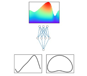
Schematic representation of the gappy DMAPs workflow: the DMAP coordinates of the full dataset are discovered. Then from partial data, the corresponding latent (DMAP) variables are inferred and, from them, it is possible to map back to the complete data.

The workflow starts by identifying a parametrization of the manifold, where the original, full dataset belongs. In this implementation, for every value of the parameter  $R$, each data point contains the wave amplitude distribution and the velocity distributions of the fluid, perpendicular to the solid–liquid interface at different points along its length
 $l$ (schematically represented with grey arrows in figure 1). Here for comparison purposes, 80 % of the dataset is used for training and the rest for testing. To derive a parsimoniously low-dimensional description of the data, the diffusion maps algorithm is implemented, as detailed in Appendix B.1. It is found by implementing the local linear regression algorithm introduced in Dsilva et al. (Reference Dsilva, Talmon, Coifman and Kevrekidis2018) and summarized in Appendix B.1, that three diffusion coordinates are enough to describe any vector in the dataset.
Then, a second round of diffusion maps is implemented, in conjunction to geometric harmonics interpolation (details can be found in Appendix B and in Evangelou et al. Reference Evangelou, Dietrich, Chiavazzo, Lehmberg, Meila and Kevrekidis2022), in order to map from any point on the reduced space to the high-dimensional ambient space.
Having established the methods for mapping between the ambient and reduced space, it is now possible, given partial information, to find first the corresponding reduced coordinates and then the entire ambient vector, including the missing information.
The accurate performance of this workflow is demonstrated in figure 10, where three cases are examined: (i) 80 points along the interface are known, from which the velocity and parameter value is recovered, with a maximum error of  $4\,\%$; (ii) 8 points, evenly distributed along the interface are known, from which again the velocity values and the parameter is recovered with a maximum error of
 $4\,\%$; (iii) 40 points are known belonging to only half of the interface shape, leading to prediction of the velocities and the parameter with a
 $4\,\%$ error.
Double DMAPS;  $R=3.5$. Each column of figures presents the actual velocity contours (a–c), predicted velocity contours (d–f) and error (g–i). The dots in the top figures signify points where the value of the amplitude is considered known. (a,d,g) The value of the amplitude at 80 points is considered known and the maximum error is
 $4\,\%$. (b,e,h) The value at 8 equidistant points is considered known and the maximum error is
 $4\,\%$. (c,f,i) The value at 40 points in the first half of the wave is considered known and the maximum error is again close to
 $4\,\%$.

The same computational experiments are conducted with gappy POD and the results are shown in figure 11. First, a POD basis is determined, based on the error (1.5  $\%$, the same as the reconstruction error achieved by DMAPs) between the reconstructed and the original test dataset, which leads to a basis with six POD vectors. The number of POD vectors required to describe the data is double the number of DMAP coordinates, suggesting that the underlying manifold is curved. The same points along the interface as before are considered known: (i) with 80 points along the interface, the maximum prediction error for the unknown velocity and parameter values is
 $10\,\%$; (ii) with 8 equidistant points along the interface, the maximum prediction error is approximately the same; (iii) when 40 points along half of the interface are considered, then the maximum error soars to
 $35\,\%$ and the predicted wave shape and velocity distribution is visibly inaccurate.
Gappy POD;  $R=3.5$. Each column of figures presents the actual velocity contours (a–c), predicted velocity contours (d–f) and error (g–i). The dots in the top figures signify points where the value of the amplitude is considered known. (a,d,g) The value of the amplitude at 80 points is considered known and the maximum error is
 $10\,\%$. (b,e,h) The value at 8 equidistant points is considered known and the maximum error is
 $10\,\%$. (c,f,i) The value at 40 points in the first half of the wave is considered known and the maximum error is close to
 $35\,\%$.

Gappy DMAPs are also successfully implemented in the case of a travelling solitary wave ( $R=20$,
 $Ca=0.00952$,
 $L=300$ and
 $\theta =6.4^\circ$) (cf. figure 12). Due to the complicated surface geometry of the solitary wave, with the presence of capillary ripples at the leading edge of the main humb, the dimensionality of the latent space, parameterized by the diffusion coordinates, is larger (four DMAPs) than in the low Reynolds case. Once the low-dimensional representation of the data is determined, it is possible to map between partial observations (i.e. interface height measurements) and the high-dimensional ambient space that includes the velocity distribution of the fluid. The prediction accuracy for the solitary wave is comparable to the low Reynolds case, leading to a maximum
 $1.5$
 $\%$ error, when 80 equidistant points are considered on the surface, which rises to
 $3\,\%$ when 40 equidistant points are considered known. When 40 points along half of the domain are considered known, then the error increases to
 $7\,\%$.
Gappy DMAPS;  $R=20$,
 $Ca=0.00952$,
 $L=300$,
 $\theta =6.4^\circ$. Each column of figures presents the predicted velocity contours (a–c) and error (d–f). The dots in the top figures signify points where the value of the amplitude is considered known. (a,d) The value of the amplitude at 80 points is considered known and the maximum error is
 $1.5\,\%$. (b,e) The value at 40 equidistant points is considered known and the maximum error is
 $3\,\%$. (c,f) The value at 40 points in the first half of the wave is considered known and the maximum error is again close to
 $7\,\%$.

5. Discussion
In this work, three different strategies for deriving accurate and economical surrogates are presented along with their application to the amplitude evolution of falling thin films.
The first option is purely data driven and physics agnostic, and relies on learning, as a black box, an amplitude PDE from observed NS data over a range of  $R$ values. In essence, the right-hand side of the PDE is substituted by an artificial neural network, which can then be integrated in time for various times, different initial conditions and parameter values.
As an alternative, we propose using a low-fidelity model, here the KS equation, in order to infuse physical intuition into the learned model. This is achieved in two different ways: the first, the additive grey box approach, uses a few high-fidelity data (results of the NS) to calibrate the KS equation, by learning an additive correction, by way of a neural network, rather than the entire right-hand side.
The second strategy, the so-called functional grey box approach, is inspired by Takens’ embedding theory, and proposes learning the accurate amplitude dynamics from a few observations of the right-hand side of an innacurate equation, such as the KS equation. Four different options are presented, utilizing either the right-hand side of the KS equation and some of its derivatives, or the value of the right-hand side operator at three points in space (at the same time instance) or in time (for the same point in space). This last approach is a demonstration of how a model that is qualitatively close to the ground truth, but quantitatively off, can be leveraged, in the data-driven era, into a more accurate and efficient learned model.
Finally, we presented a gappy DMAP methodology, the nonlinear counterpart of gappy POD, which allows us to infer quantities that are inaccessible to measuring devices, such as the velocity profile of the fluid below the surface, when only some measurements are known, such as the height of the thin film at certain points. This may be trivial for low  $R$ values, since the interface height is ‘slaved’ to the velocity. Nevertheless, for slightly higher
 $R$ values, the amplitude is no longer a function of just the position; hence, surrogate models with more than one equation become necessary in this flow regime (Chang Reference Chang1986; Oron & Gottlieb Reference Oron and Gottlieb2002; Kalliadasis et al. Reference Kalliadasis, Ruyer-Quil, Scheid and Velarde2012; Shklyaev & Nepomnyashchy Reference Shklyaev and Nepomnyashchy2017).
The benefits of the proposed approach are twofold: nonlinear manifold learning methods, such as DMAPs, yield a more parsimonious description of the manifold, requiring only a few coordinates to accurately reconstruct the original data. In contrast, we demonstrate that gappy POD requires higher-dimensional hyperplanes to span the data. The second advantage of gappy DMAPs is related to the choice of known values. Some consideration is necessary for choosing points that contain rich enough information in order to achieve accurate reconstruction; it is, nevertheless, less sensitive to the position of the provided measurements than its linear counterpart.
Funding
This work was partially supported by the US AFOSR and by the US DOE (IGK). CML received the support of a ‘la Caixa’ Foundation Fellowship (ID 100010434), code LCF/BQ/AA19/11720048. EDK received funding from the European Union's Horizon 2020 research and innovation programme under the Marie Skłodowska-Curie grant agreement No 890676 - DataProMat.
Declaration of interests
The authors report no conflict of interest.
Author contributions
C.M.L. performed computational analyses, interpreted the data and wrote the manuscript, Y.P. performed computational analyses and wrote the manuscript, G.K. developed the computational fluid dynamics model, contributed to mathematical analyses and wrote the manuscript, E.D.K. performed computational analyses, interpreted the data and wrote the manuscript and I.G.K. conceived the research, supervised the study and wrote the manuscript.
Appendix A. Transformations between NS and KS equations scales
The  $(x,t)$ NS frame of reference is mapped on the KS
 $(\xi,\tau )$ through the expressions
 \begin{equation} \xi=\epsilon(x-Ft) \quad \text{and} \quad \tau = \frac{\epsilon^4 W F}{12} t, \end{equation}
while the interfacial height,  $h(x,t)$, is related to the amplitude
 $\phi (\xi,\tau )$ as
 \begin{equation} h(x,t) \approx 1+\epsilon\frac{RF}{15}\phi(\xi,\tau). \end{equation}
To be able to compare the results between NS and KS equations, we employ the chain rule and derive the appropriate transformations for the time and spatial derivatives. To transform NS data to the KS formulation, the following expressions can be used:
 \begin{equation} \left.\begin{array}{c} \displaystyle\dfrac{\partial^{\beta} \phi}{\partial \xi^{\beta}}=\dfrac{1}{\epsilon^{\beta+1}}\dfrac{15}{RF}\dfrac{\partial^{\beta} h}{\partial x^{\beta}},\\ \displaystyle\dfrac{\partial \phi}{\partial \tau}=\dfrac{180}{\epsilon^5 W R F^2}\dfrac{\partial h}{\partial t}+\dfrac{180}{\epsilon^5 W R F}\dfrac{\partial h}{\partial x}. \end{array}\right\} \end{equation}
Inversely, to map KS data to the NS formulation, the following expressions can be used:
 \begin{equation} \left.\begin{array}{c} \displaystyle\dfrac{\partial^{\beta} h}{\partial x^{\beta}}=\epsilon^{\beta+1}\dfrac{R F}{15}\dfrac{\partial^{\beta} \phi}{\partial \xi^{\beta}},\\ \displaystyle\dfrac{\partial h}{\partial t}={-}\dfrac{\epsilon^2 R F^2}{15}\dfrac{\partial \phi}{\partial \xi}+\dfrac{\epsilon^5 W R F^2}{180}\dfrac{\partial \phi}{\partial \tau}. \end{array}\right\} \end{equation}
Appendix B. Diffusion maps and gappy POD
B.1. Diffusion maps
Diffusion maps (Coifman & Lafon Reference Coifman and Lafon2006; Nadler et al. Reference Nadler, Lafon, Coifman and Kevrekidis2006; Coifman et al. Reference Coifman, Kevrekidis, Lafon, Mauro and Nadler2008) are a framework that can (based upon diffusion processes) facilitate discovering meaningful low-dimensional intrinsic geometric descriptions of datasets, even when the data are high dimensional, nonlinear and/or corrupted by (relatively small) noise. The method is based on the construction of a Markov transition probability matrix, corresponding to a random walk, on a graph whose vertices are the data points, with transition probabilities being the local similarities between pairs of data points. The leading few eigenvectors of the Markov matrix can be used as data-driven coordinates that provide a reparametrization of the data. To construct a low-dimensional embedding for a dataset  $\boldsymbol {X}$ of
 $M$ individual points (represented as
 $d$-dimensional real vectors
 $x_1,\ldots, x_M$), a similarity measure
 $d_{ij}$ between each pair of vectors
 $x_i, x_j$ is computed. The standard Euclidean distance or the Euclidean norm may be considered to this end. By using this similarity measure, an affinity matrix is constructed. A popular choice is the Gaussian kernel
 \begin{equation} w(i,j)=\exp\left[-\left(\frac{\|x_i-x_j\|}{\epsilon_{\delta}}\right)^2\right], \end{equation}
where  $\epsilon _{\delta }$ defines a scale hyperparameter that quantifies the local similarity for each data point. To recover a parametrization regardless of the sampling density, the normalization
 \begin{equation} \tilde{\boldsymbol{W}} = \boldsymbol{P}^{-\alpha} \boldsymbol{W} \boldsymbol{P}^{-\alpha} \end{equation}
is performed, where  $P_{ii} = \sum _{j=1}^M W_{ij}$ and
 $\alpha =1$ to factor out the density effects. A second normalization applied on
 $\tilde {\boldsymbol {W}}$,
 \begin{equation} \boldsymbol{K}=\boldsymbol{D}^{{-}1} \tilde{\boldsymbol{W}}, \end{equation}
gives a  $M\times M$ Markov matrix
 $\boldsymbol {K}$, where
 $\boldsymbol {D}$ is a diagonal matrix, collecting the row sums of matrix
 $\tilde {\boldsymbol {W}}$. The stochastic matrix
 $\boldsymbol {K}$ has a set of real eigenvalues
 $1=\lambda _1\geq \cdots \geq \lambda _M$ with corresponding eigenvectors
 $\phi _i$. To check if model (variable) reduction can be achieved, the number of retained eigenvectors has to be appropriately truncated. In practice, it is useful to consider that not all obtained eigenvectors parametrize independent directions, but rather most of them can be considered as spanning the same directions with different frequencies. Eigenvectors that parametrize the same directions in this context are called harmonics and those that parametrize independent directions non-harmonics. A minimal representation of the DMAP space is made possible by carefully selecting the non-harmonic coordinates, which do not necessarily correspond to the most dominant eigenmodes of the Markov matrix. This is a stark difference between diffusion maps and its linear counterpart, POD or principal component analysis, where the dominant modes are retained for the truncated representation of the data. If the number of the non-harmonic eigenvectors is less than the number of ambient space dimensions, then model (variable) reduction is achieved.
A proposed algorithm for identifying the non-harmonic eigenvectors is presented in Dsilva et al. (Reference Dsilva, Talmon, Coifman and Kevrekidis2018), based on local linear regression. In a nutshell, a local linear function is used in order to fit the DMAP coordinate  $\phi _k$ as a function,
 $f$, of the previous vectors
 $\tilde {\varPhi }_{k-1}= [\phi _1,\phi _2,\ldots,\phi _{k-1}]$. If
 $\phi _k$ can be accurately expressed as a function of the other DMAP coordinates, then it does not represent a new direction on the dataset, and is omitted for dimensionality reduction. On the contrary, if
 $\phi _k$ cannot be expressed as a function of the previous eigenvectors then
 $\phi _k$ is a new independent eigendirection that must be retained for a parsimonious representation of the data. To quantify the accuracy of the fit, the following metric is used:
 \begin{equation} r_k=\sqrt{\frac{\displaystyle\sum_{i=1}^{n}(\phi_k(i)-f(\tilde{\varPhi}_{k-1}(i)))^2} {\displaystyle\sum_{i=1}^{n}(\phi_k(i))^2)}}. \end{equation}
A small value of  $r_k$ is associated with a
 $\phi _k$ that is a harmonic function of the previous eigenmodes, whereas a higher value of
 $r_k$ signifies that
 $\phi _k$ is a new independent direction on the data manifold. It has been shown in Dsilva et al. (Reference Dsilva, Talmon, Coifman and Kevrekidis2018) that selecting only the eigenvectors that correspond to higher values of
 $r_k$ leads to a parsimonious representation of the data. Eventually, the vector
 $x_i$ is mapped to a vector whose first component is the ith component of the first selected non-trivial eigenvector, whose second component is the ith component of the second selected non-trivial eigenvector, and so on.
To map a new point,  $x_{new}$, from the ambient space to DMAP space, a mathematically elegant approach known as the Nyström extension, introduced in (Coifman & Lafon Reference Coifman and Lafon2006) is used, summarized here for completeness. The starting point of the Nyström extension is to compute the distances,
 $d({{\cdot }, x_{new}})$, between the new point,
 $x_{new}$, and the
 $M$ data points in the original dataset, the same normalizations used for DMAP need to also be applied here. The Nyström extension formula reads
 \begin{equation} \phi_j(x_{new})=\lambda_j^{{-}1}\sum_{i=1}^{M}\tilde{k}(x_i,x_{new})\phi_{j}(x_{i}), \end{equation}
where  $\lambda _j$ is the jth eigenvector and
 $\phi _j(x_i)$ is the ith component of the
 $j$th eigenvector.
B.2. Geometric harmonics
Geometric harmonics was introduced in Coifman & Lafon (Reference Coifman and Lafon2006), inspired by the Nyström extension as a scheme for extending functions defined on data  $\boldsymbol {X}$,
 $f(\boldsymbol {X}):\boldsymbol {X} \to \mathbb {R}$, for
 $x_{new} \notin \boldsymbol {X}$. This out-of-sample extension is achieved by using a particular set of basis functions called geometric harmonics. These functions are computed as eigenvectors of the symmetric
 $M\times M$
 $\boldsymbol {W}$ matrix. The eigendecomposition of the symmetric and positive semidefinite matrix
 ${\mathbf {W}}$ leads to a set of orthonormal eigenvectors
 $\mathbf {\psi }_1,\mathbf {\psi }_2, \ldots, \mathbf {\psi }_M$ with non-negative eigenvalues
 $\sigma _1 \geq \sigma _2 \geq \cdots \geq \sigma _M \geq 0$.
From this set of eigenvectors, to avoid numerical issues, we consider a truncated subset  $S_\delta = (\alpha : {\sigma _{\alpha }\geq \delta \sigma _1})$ where
 $\delta >0$. The extension of
 $f$ for a new point
 $x_{new}$ is accomplished by first projecting the function of interest in the (truncated) computed set of eigenvectors
 \begin{equation} f\rightarrow P_\delta f =\sum_{\alpha\in S_\delta}\langle\, f,\psi_\alpha \rangle \psi_\alpha \end{equation}
and then extending the function  $f$ for
 $x_{new} \notin \boldsymbol {X}$,
 \begin{equation} (Ef)(x_{new})= \sum_{\alpha \in S_{\delta}}\langle\, f,\psi_{\alpha} \rangle\varPsi_\alpha(x_{new}), \end{equation}
where
 \begin{equation} \varPsi_\alpha(x_{new})=\lambda_\alpha^{{-}1}\sum_{i=1}^{M}w(x_{new},x_i)\psi_{\alpha}(x_{i}) \end{equation}
and
 \begin{equation} w(x_{new},x_i)=\exp\left[-\left(\frac{d_i}{\tilde{\epsilon}}\right)^2\right],\quad d_i=\|x_{new} - x_i\|_2. \end{equation}
B.3. Double diffusion maps and their latent harmonics
A slight twist of the geometric harmonics (Evangelou et al. Reference Evangelou, Dietrich, Chiavazzo, Lehmberg, Meila and Kevrekidis2022) is presented in this section. As discussed above, geometric harmonics constructs an input–output mapping between the ambient coordinates  $\boldsymbol {X}$ and a function of interest
 $f$ defined on
 $\boldsymbol {X}$. However, it is possible, if the data are lower dimensional, to construct a map in terms of only the non-harmonic eigenvectors. This is achieved similar to the traditional geometric harmonics, by firstly constructing an affinity matrix
 \begin{equation} \bar{w}(i,j)=\exp\left[-\left(\frac{\|\phi_i-\phi_j\|}{\epsilon^\star}\right)^2\right]. \end{equation}
In this case, the affinity matrix is constructed in terms of only the non-harmonic DMAPs coordinates. To distinguish the notation between geometric harmonics and double diffusion maps, we will use  $\bar {\psi }$. As in the traditional geometric harmonics, the function
 $f$ is projected to a truncated set of the obtained eigenvectors
 \begin{equation} f\rightarrow P_\delta f =\sum_{\beta\in \overline{S}_\delta}\langle\, f,\overline{\psi}_\beta \rangle \overline{\psi}_\beta. \end{equation}
The extension of  $f$ for
 $\mathbf {\phi }_{new}$ is achieved by firstly extending the values of the geometric harmonic functions
 $\varPsi _{\beta }$ for
 $\mathbf {\phi }_{new},$
 \begin{equation} \overline{\varPsi}_\beta(\boldsymbol{\phi}_{new})=\overline{\sigma}_\beta^{{-}1} \sum_{i=1}^{M}\bar{w}(\phi_{new},\phi_i)\overline{\psi}_{\beta}(\boldsymbol{\phi}_{i}), \end{equation}
and then estimating the value of  $f$ at
 $\mathbf {\phi }_{new}$,
 \begin{equation} (Ef)(\boldsymbol{\phi}_{new})= \sum_{\beta \in \overline{S}_{\delta}}\langle\, f,\overline{\psi}_{\beta} \rangle\overline{\varPsi}_\beta(\boldsymbol{\phi}_{new}). \end{equation}
B.4. Gappy POD
In this section the gappy POD method is summarized for completeness. Consider a dataset  $\boldsymbol {X}$ of
 $M$ vectors (represented as
 $d$-dimensional real vectors
 $x_1,\ldots, x_M$). A POD basis,
 $\mathbf {\varPhi } \in \Re ^{N \times M}$, of
 $\boldsymbol {X}$ is computed, such that
 $\boldsymbol {X}$ can be approximated as a linear combination of
 $\boldsymbol {p}$ vectors, i.e.
 \begin{equation} \tilde{\boldsymbol{X}}= \sum_{j=1}^{p} c^j\mathbf{\varPhi}^j \end{equation}
or in matrix-vector format,
 \begin{equation} \tilde{\boldsymbol{X}}=\mathbf{\varPhi} {\cdot} c. \end{equation}
The size of the truncated POD basis  $\mathbf {\varPhi }$ is selected based on the error between the actual vector
 $\boldsymbol {X}$ and the reconstructed approximation
 $\tilde {\boldsymbol {X}}$,
 \begin{equation} \text{Reconstruction error } = \lVert \boldsymbol{X}-\tilde{\boldsymbol{X}} \rVert. \end{equation}
Consider now a vector  $X'$ that is spanned by the same basis
 $\varPhi$ and that only
 $m$ values of this vector are known, so that the partial vector
 $X_{partial}'$ can be defined as
 \begin{equation} X_{partial}'=m {\cdot} X', m \in \Re^{m\times N}. \end{equation}
The goal is to find coefficients  $c'$, such that an approximation
 $\widetilde {X'}$ of the vector
 $X'$ can be defined as
 \begin{equation} \widetilde{X'}=X' {\cdot} c'; \end{equation}
then
 \begin{equation} X_{partial}' \approx m {\cdot} X' {\cdot} c'. \end{equation}
Finding the values of  $c'$ that satisfy the above leads to an optimization problem solved through the linear system
 \begin{equation} M {\cdot} c' = (m {\cdot} \mathbf{\varPhi})' {\cdot} X_{partial}', \end{equation}
with  $M = (m {\cdot } \mathbf {\varPhi })' {\cdot } (m {\cdot } \mathbf {\varPhi })$.


 Open access

