1. Introduction
Closed-loop flow control is of major academic and industrial interest. At the interface of control theory and fluid mechanics it is pertinent to many engineering domains, such as aeronautics and combustion. It can be used to reduce aerodynamic drag of an automobile or an airplane, increase combustion efficiency, or enhance mixing. Control of amplifier flows like boundary layers, mixing layers, jets or separated flows is particularly relevant and challenging. Indeed, amplifier flows are globally stable, however convective instabilities will amplify disturbances while being advected downstream (Marquet et al. Reference Marquet, Sipp, Chomaz and Jacquin2008; Brandt et al. Reference Brandt, Sipp, Pralits and Marquet2011). Incoming perturbations are likely to be amplified to the point where they disrupt the entire flow. Nullifying these disturbances before they can be amplified by the flow is a great challenge for the flow control community (Schmid & Henningson Reference Schmid and Henningson2001). Typically when considering a laminar amplifier flow, the control objective can be to inhibit the transition to turbulence. Examples of such flows abound, a much-studied amplifier flow being that over a backward-facing step (BFS) (Barkley, Gomes & Anderson Reference Barkley, Gomes and Anderson2002; Blackburn, Barkley & Sherwin Reference Blackburn, Barkley and Sherwin2008) which presents an unsteady region of convective instability. Another example is that of the flow over a cavity, used for studying the control of global instabilities (Rowley & Williams Reference Rowley and Williams2006).
Control of amplifier flows has been the subject of much research (Hervé et al. Reference Hervé, Sipp, Schmid and Samuelides2012; Belson et al. Reference Belson, Semeraro, Rowley and Hennginson2013). A control law can be computed in one of two ways. One possibility is to compute the model using previous knowledge of the physics of the flow (Sipp et al. Reference Sipp, Marquet, Meliga and Barbagallo2010). When derived directly from the Navier–Stokes equations these models are of very high order and require reduction before they can be used in a realistic setting. Model reduction is still a rich and very active research field, see Efe & Ozbay (Reference Efe and Ozbay2003), Rowley, Colonius & Murray (Reference Rowley, Colonius and Murray2004) and Akervik et al. (Reference Akervik, Hoepffner, Ehrenstein and Henningson2007). In some cases a physical analysis of the flow can yield simple models leading to efficient control laws as shown in Pastoor et al. (Reference Pastoor, Henning, Noack, King and Tadmor2008) and Gautier & Aider (Reference Gautier and Aider2014a ). The second option is system identification as suggested by Ljung (Reference Ljung1999). In this case, the flow is probed until a model can be derived from its responses. This approach is data based: it seeks to build an input–output model for the flow from empirical observations. Such an approach has been applied with success to the control of the recirculation bubble behind a BFS, see Becker et al. (Reference Becker, Garwon, Gutknecht, Barwolff and King2005) and Henning & King (Reference Henning and King2007).
The BFS is considered as a benchmark geometry for the study of amplifier flows: separation is imposed by a sharp edge creating a strong shear layer susceptible to Kelvin–Helmholtz instability. Upstream perturbations are amplified in the shear layer leading to significant downstream disturbances. This flow has been extensively studied both numerically and experimentally (Armaly et al. Reference Armaly, Durst, Pereira and Schonung1983; Hung, Parviz & John Reference Hung, Parviz and John1997; Beaudoin et al. Reference Beaudoin, Cadot, Aider and Wesfreid2004; Aider, Danet & Lesieur Reference Aider, Danet and Lesieur2007).
The principle of feed-forward control is to act on the flow upon detection of an event as opposed to the more common feed-back control where one reacts to an event. Feed-forward algorithms have been successfully used in flow control in numerical simulations (Belson et al. Reference Belson, Semeraro, Rowley and Hennginson2013). Recently Hervé et al. (Reference Hervé, Sipp, Schmid and Samuelides2012) have shown the effectiveness of a feed-forward algorithm computed using an auto-regressive moving-average exogenous model (ARMAX) to capture the relevant dynamics of the flow. The resulting control law leads to reduced energy levels and fluctuations. The aim of this work is to determine the feasibility and robustness of this approach in an experimental setting, a perturbed backward-facing step flow.
2. Experimental set-up
2.1. Water tunnel
Experiments were carried out in a hydrodynamic channel in which the flow is driven by gravity. The flow is stabilized by divergent and convergent sections separated by honeycombs. The quality of the main stream can be quantified in terms of flow uniformity and turbulence intensity. The standard deviation
 ${\it\sigma}$
is computed for the highest free-stream velocity featured in our experimental set-up. We obtain
 ${\it\sigma}=0.059\ \text{cm}\ \text{s}^{-1}$
which corresponds to turbulence levels of
 ${\it\sigma}/U_{\infty }=0.0023$
. For the present experiment the flow velocity is
 $U_{\infty }=2.1\ \text{cm}\ \text{s}^{-1}$
giving a Reynolds number based on step height
 $Re_{h}=U_{\infty }h/{\it\nu}=430$
, where
 ${\it\nu}$
is kinematic viscosity. Following the assumptions of Hervé et al. (Reference Hervé, Sipp, Schmid and Samuelides2012) the Reynolds number was chosen to ensure a sub-critical linear two-dimensional flow.
2.2. Backward-facing step geometry and upstream perturbation
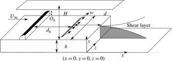
The BFS geometry and the main geometric parameters are shown in figure 1. BFS height is
 $h=1.5\ \text{cm}$
. Channel height is
 $H=7\ \text{cm}$
for a channel width
 $w=15\ \text{cm}$
. The vertical expansion ratio is
 $A_{y}=H/(h+H)=0.82$
and the spanwise aspect ratio is
 $A_{z}=w/(h+H)=1.76$
. The injection slot is located
 $d/h=2$
upstream of the step edge.
Sketch of the BFS geometry and definition of the main parameters.

The principle of the method described in Hervé et al. (Reference Hervé, Sipp, Schmid and Samuelides2012) is to devise an input–output model for the flow based on experimental data. This model is used to compute actuation aimed at negating incoming upstream noise, thereby preventing its amplification. Because our sensor is two-dimensional in the symmetry plane and our actuator can only deliver span-wise homogeneous actuation, a two-dimensional upstream perturbation is required for effective control. As shown in figure 1 a two-dimensional obstacle with a rounded leading edge of height
 $O_{h}=0.8\ \text{cm}$
has been placed at
 $d_{h}=15\ \text{cm}$
upstream from jet injection (
 $12h$
from the step edge) to perturb the flow. Because of the low Reynolds number the flow stays two-dimensional.
2.3. Sensor: two-dimensional real-time velocity field computations
The sensors used as inputs for the closed-loop experiments are visual sensors, i.e. regions of the two-dimensional PIV (particle image velocimetry) velocity fields measured in the symmetry plane as shown in figure 4 below. The flow is seeded with
 $20\ {\rm\mu}\text{m}$
neutrally buoyant polyamid seeding particles. They are illuminated by a laser sheet created by a 2 W continuous laser beam operating at
 ${\it\lambda}=532\ \text{nm}$
. Images of the vertical symmetry plane are recorded using a Basler acA 2000–340 km 8 bit CMOS camera. Velocity field computations are run on a Gforce GTX 580 graphics card. The algorithm used to compute the velocity fields is based on a Lukas–Kanade optical flow algorithm called FOLKI developed by Besnerais & Champagnat (Reference Le Besnerais and Champagnat2005). Its offline and online accuracy has been demonstrated and detailed by Champagnat et al. (Reference Champagnat, Plyer, Le Besnerais, Leclaire, Davoust and Le Sant2011) and Gautier & Aider (Reference Gautier and Aider2014b
). Furthermore this acquisition method was successfully used in Davoust, Jacquin & Leclaire (Reference Davoust, Jacquin and Leclaire2012) and Gautier & Aider (Reference Gautier and Aider2013). The size of the velocity fields is
 $17.2\ \text{cm}\times 4.6\ \text{cm}$
. They are computed every
 ${\it\delta}_{t}=40\ \text{ms}$
, for a sampling frequency
 $F_{s}=25\ \text{Hz}$
.
2.4. Uncontrolled flow
The swirling strength criterion
 ${\it\lambda}_{Ci}$
is an effective way of detecting vortices in two-dimensional velocity fields, introduced and improved by Chong, Perry & Cantwell (Reference Chong, Perry and Cantwell1990) and Zhou et al. (Reference Zhou, Adrian, Balachandar and Kendall1999). For two-dimensional data the swirling criterion is defined as
 ${\it\lambda}_{Ci}=\sqrt{4\det (\boldsymbol{{\rm\nabla}}\boldsymbol{ u })-\text{tr}(\boldsymbol{{\rm\nabla}}\boldsymbol{ u })^{2}}/2$
(when this quantity is real).
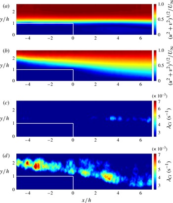
Figure 2(a,b) shows the mean velocity amplitude fields for the perturbed (with obstacle) and unperturbed (without obstacle) flows. Figure 2(c,d) shows corresponding
 ${\it\lambda}_{Ci}$
snapshots, highlighting the perturbations caused by the upstream obstacle. Figure 2(d) shows the steady stream of vortices created by the obstacle interacting with the recirculation. Quantitatively,
 ${\it\lambda}_{Ci}$
in the perturbed flow is an order of magnitude higher than in the flow unperturbed flow. The boundary layer thicknesses at the step edge for the flow with and without obstacles are
 ${\it\delta}=1.34h$
and
 ${\it\delta}=1.73h$
respectively.
Mean velocity magnitude contour fields for the unperturbed (a) and perturbed (b) flow. Instantaneous snapshots showing contours of
 ${\it\lambda}_{Ci}$
for the unperturbed (c) and perturbed (d) flow.

Turbulent kinetic energy (TKE) is defined as
 $k(x,y,t)=(u^{\prime }(x,y,t)^{2}+v^{\prime }(x,y,t)^{2})/2$
, where
 $u^{\prime }$
,
 $v^{\prime }$
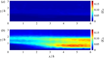
are longitudinal and vertical velocity fluctuations. Figure 3(a) shows the time-averaged TKE field
 $\langle k(x,y)\rangle _{t}$
downstream of the step for the unperturbed case, while figure 3(b) shows the perturbed case. The field exhibits two regions of high TKE. The lower region corresponds to the perturbation-induced recirculation bubble. The upper region corresponding to perturbations induced by vortices shed by the upstream obstacle.
TKE field
 $\langle k(x,y)\rangle _{t}$
downstream of the BFS: unperturbed (a) perturbed (b).

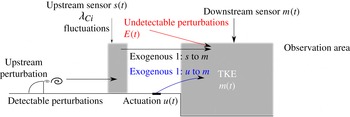
Schematic description of the main terms used in the ARMAX model.

2.5. Actuation
In Hervé et al. (Reference Hervé, Sipp, Schmid and Samuelides2012) actuation is a Gaussian flow sink/source placed above the step, which is not physically feasible. In our case, actuation is provided by a flush slot jet, 0.1 cm long and 9 cm wide. This actuation has been chose to obtain a perturbation as homogeneous along the spanwise direction as possible. The jet angle to the wall is 45°. The slot is located 3 cm (
 $2h$
) upstream of the step edge (figure 1). Jet flow is induced using water from a pressurized tank. It enters a plenum and goes through a volume of glass beads designed to homogenize the incoming flow. Jet amplitude is controlled by changing tank pressure. Because channel pressure is higher than atmospheric pressure this allows us to provide both blowing and suction. The convection time from jet injection to measurement area is 2 s (
 ${<}0.5\ \text{Hz}$
). The maximum actuation frequency
 $f_{a}$
is approximately 1 Hz which is sufficient for these experiments.
The control law output is velocities, and these are converted into pressure commands using a pre-calibrated transfer function.
3. ARMAX model
3.1. Introduction
An ARMAX model is used because it can be derived from experimental data (Pamart et al. Reference Pamart, Dandois, Garnier and Sagaut2010). Furthermore it has been shown by Hervé et al. (Reference Hervé, Sipp, Schmid and Samuelides2012) that it is particularly well adapted at modelling the BFS flow when in the linear regime.
Two exogenous inputs
 $s(t),u(t)$
and one output
 $m(t)$
are used. The first exogenous input
 $s(t)$
measures fluctuations of spatially averaged
 ${\it\lambda}_{Ci}$
(small grey area on figure 4). Such a sensor is well suited to the detection of upstream vortices created by the obstacle. The second exogenous input is jet to cross-flow velocity ratio
 $u(t)$
.
Output
 $m(t)$
is a measure of TKE fluctuations in the recirculation region. The control objective is to negate the incoming perturbations created by the obstacle in order to reduce overall downstream TKE fluctuations. TKE is averaged over the whole downstream velocity field (large grey area on figure 4):
 $$\begin{eqnarray}m(t)=\frac{\displaystyle \int k(x,y,t)\text{d}x\text{d}y}{\displaystyle \int \text{d}x\text{d}y}.\end{eqnarray}$$
Following Hervé et al. (Reference Hervé, Sipp, Schmid and Samuelides2012) the equation for the model is defined as:
 $$\begin{eqnarray}\displaystyle & \underbrace{m(t)+\mathop{\sum }\limits_{k=1}^{n_{a}}a_{k}m(t-k)}_{\text{auto-regressive}}=\underbrace{\mathop{\sum }\limits_{k=n_{du}}^{n_{du}+n_{bu}}b_{k}^{u}u(t-k)}_{\text{exogenous}1}+\underbrace{\mathop{\sum }\limits_{k=n_{ds}}^{n_{ds}+n_{bs}}b_{k}^{s}s(t-k)}_{\text{exogenous}2}+\,E(t), & \displaystyle\end{eqnarray}$$
 $$\begin{eqnarray}\displaystyle & E(t)=\underbrace{\mathop{\sum }\limits_{k=n_{1}}^{n_{c}}c_{k}e(t-k)}_{\text{moving average}}+\,e(t). & \displaystyle\end{eqnarray}$$
To achieve feed-forward control, the effects of upstream sensing
 $s(t)$
and actuation
 $u(t)$
on the output
 $m(t)$
must be quantified. For a pure feed-forward control, upstream estimation should be independent of actuation, see Semeraro (Reference Semeraro2013). During control,
 $u(t)$
is a function of
 $s(t)$
. For our experimental set-up we found that interference between actuation and the upstream sensor caused the control to saturate actuation. To avoid this effect, an inclined jet has been used instead of a wall normal jet. Moreover since
 $s(t)$
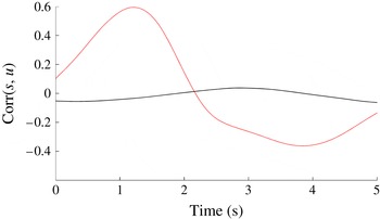
only measures the presence of vortices it is weakly affected by downstream actuation compared to vertical velocity for example. Special care must be taken to lower actuation amplitude as much as possible so that it does not affect the upstream sensor. Figure 5 shows the cross-correlation function between
 $s(t)$
and
 $u(t)$
for two cases: the calibration case and a case where there is interference (jet amplitude is too high) between the upstream sensor and the actuator. Interference results in high correlation between
 $s$
and
 $u$
whereas in our calibration case correlation is negligible.
Cross-correlation functions between
 $s(t)$
and
 $u(t)$
for the calibration case (black) and a case with interference between the upstream sensor and the actuator (grey).

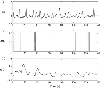
Calibration time series. (a)
 $s(t)$
captures the influence of upstream disturbances; (b)
 $u(t)$
pseudo-random control law; (c)
 $m(t)$
spatially averaged downstream TKE, mean value has been removed.

Coefficients
 $(a_{k},b_{k}^{u},b_{k}^{s})$
are computed to minimize error
 $e(t)$
at all times. To calibrate the model the user must provide time series for both inputs and outputs, the longer the better. Values for
 $n_{a},n_{du},n_{bu},n_{ds},n_{bs}$
are tied to the physics of the flow and are determined by the user. These coefficients are linked to time delays in the flow system. The flow time history required for the model to work properly is given by
 $n_{a}{\it\delta}_{t}$
(auto-regressive part). Here
 $n_{du}{\it\delta}_{t}$
and
 $n_{ds}{\it\delta}_{t}$
are the times required for the respective inputs to affect the output; they are linked to flow convective velocity. Also,
 $n_{bu}{\it\delta}_{t}$
and
 $n_{bs}{\it\delta}_{t}$
represent input time scales. They correspond to the time during which upstream effects affect the output signal. Finally
 $n_{c}$
is used to model noise and ensures robustness (Hervé et al.
Reference Hervé, Sipp, Schmid and Samuelides2012). This value is chosen iteratively, once all other coefficients have been fixed, to get the best possible fit between experimental data and model output.
3.2. Model computation
Figure 6 shows a small segment of the calibration time series. The forcing law
 $u(t)$
used in these series is one of pseudo-random pulses. Pulses are made to occur at random intervals, long enough for the effects of the previous pulse to have subsided before the next pulse. During these intervals the only input to the system is
 $s(t)$
. This allows the effects of actuation and upstream perturbations to be computed using a single time series. Impulse amplitude for actuation
 $u(t)$
should be chosen such that it is high enough to affect the output
 $m(t)$
but low enough to avoid perturbations of the upstream output
 $s(t)$
. The mean value was removed for
 $m(t)$
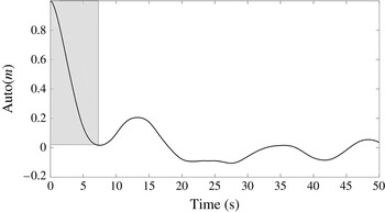
because the focus is on suppressing fluctuations in the output. Calibration data were acquired over 25 min. Figure 7 shows the auto-correlation function for
 $m(t)$
. A quasi-oscillatory behaviour can be observed. It can be used to choose
 $n_{a}$
which is such that
 $n_{a}{\it\delta}_{t}$
equals half the oscillatory period, as recommended by Hervé et al. (Reference Hervé, Sipp, Schmid and Samuelides2012).
Auto-correlation function for
 $m(t)$
.

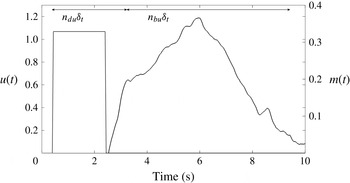
Figure 8 shows the response to an impulse, which can be used to evaluate the coefficients
 $n_{du},n_{bu},n_{ds},n_{bs}$
. The time delay
 $t_{du}=2.5\ \text{s}$
between the beginning of the actuation and the response gives
 $t_{du}=n_{du}{\it\delta}_{t}$
. The upstream sensor is located 3.5 cm upstream of the jet injection. Assuming perturbations travel at channel velocity, this implies a time delay of
 $t_{ds}\approx 1.7\ \text{s}$
for an upstream disturbance to affect the output, thus
 $n_{ds}{\it\delta}_{t}=t_{du}+t_{ds}$
.
Output impulse response.

Let
 $t_{bu}$
be the time during which an impulse in
 $u$
affects the output, as shown in figure 8, then
 $n_{bu}{\it\delta}_{t}=t_{bu}$
. Because the response to an impulse in
 $s$
is more difficult to distinguish we assume
 $n_{bs}=n_{bu}$
. Finally
 $n_{c}$
is chosen after the other coefficients have been fixed in order to get the best possible agreement between model and real outputs. Table 1 summarizes the final coefficients used in the computation of the ARMAX model using the Matlab armax function (Ljung Reference Ljung1999); it also shows the corresponding time delays and averages in seconds.
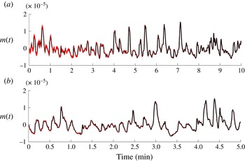
(a) Calibration data set, model performance (dotted grey) compared to experimental results (in black). (b) Validation data set, model performance (dotted grey) compared to experimental results (in black).

Figure 9(a) compares ARMAX output to the source signal for the calibration series. Agreement is good at 96 %. Figure 9(b) compares ARMAX output to the source signal for the validation series; agreement is slightly lower at 94 %. Here
 $s,u,m$
are initialized at zero, which explains the poorer agreement at the start.
ARMAX coefficients.

3.3. Linearity
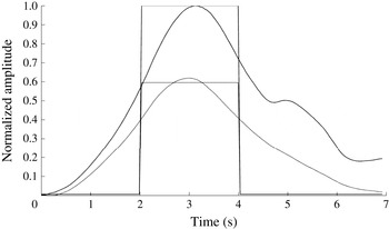
A major underlying assumption of this approach is the linearity of the system. In our set-up this was checked by imposing periodic pulsed forcing, for two different amplitudes. For both amplitudes, the response in
 $m(t)$
was averaged over each impulse. This phase-averaged response is shown in figure 10. Impulse amplitude ratio is also given for comparison. The signals were shifted in time to facilitate comparison. Figure 10 shows how a change in impulse amplitude leads to a proportional change in response amplitudes, confirming the linear behaviour of the flow. Linearity was also checked when varying the size of the window where TKE is computed. Averaging over smaller windows, closer to the step, where nonlinearities are weaker, did not improve system linearity.
Time evolutions of
 $m(t)$
in response to two short impulses (square signals) of different amplitudes (thick and thin lines). The signals have been shifted in time to better highlight the linear nature of the response.

4. Results
4.1. Control law
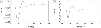
Figure 11(a,b) shows the impulse response for both exogenous inputs. These plots show that impulse responses are qualitatively similar; however they differ in amplitude.
ARMAX impulse response for (a) exogenous input
 $s(t)$
and (b) exogenous input
 $u(t)$
.

Impulses responses can help determine if a model is ‘controllable’ and whether or not the objective (negating TKE fluctuations) is a priori attainable, which makes them an invaluable diagnostics tool. To achieve fluctuation suppression the control law suggested by Hervé et al. (Reference Hervé, Sipp, Schmid and Samuelides2012) was computed.
Only perturbations detected in
 $s(t)$
can potentially be cancelled out. Other sources of disturbance are not modelled and are ignored by the control law. The following equation illustrates how the output signal can be written as a combination of the input signals:
 $$\begin{eqnarray}m(t)=\mathop{\sum }\limits_{k=0}^{\infty }h_{k}^{s}s(t-k)+h_{k}^{u}u(t-k).\end{eqnarray}$$
The coefficients
 $h_{k}^{s},h_{k}^{u}$
are obtained by computing the impulse response of the ARMAX model for an impulse response
 $s(t=0)=1,u(t=0)=1$
:
 $$\begin{eqnarray}\displaystyle & \forall km_{impulses}(t=k)=h_{k}^{s}s(0), & \displaystyle\end{eqnarray}$$
 $$\begin{eqnarray}\displaystyle & \forall km_{impulseu}(t=k)=h_{k}^{u}u(0). & \displaystyle\end{eqnarray}$$
These coefficients can be used to express
 $m(t)$
as a function of
 $s(t),u(t)$
as shown in (4.4) as follows:
 $$\begin{eqnarray}\boldsymbol{M}_{Nt}=\boldsymbol{\mathsf{H}}_{u}\boldsymbol{U}^{f}+\boldsymbol{\mathsf{G}}_{u}\boldsymbol{U}^{P}+\boldsymbol{\mathsf{G}}_{s}\boldsymbol{S}^{P},\end{eqnarray}$$
with
 $$\begin{eqnarray}\boldsymbol{M}_{Nt}=\left(\begin{array}{@{}c@{}}m_{t}\\ m_{t+1}\\ \vdots \\ m_{t+Nt}\end{array}\right),\quad \boldsymbol{U}^{f}=\left(\begin{array}{@{}c@{}}u_{t}\\ u_{t+1}\\ \vdots \\ u_{t+Nt}\end{array}\right),\quad \boldsymbol{U}^{P}=\left(\begin{array}{@{}c@{}}u_{t-1}\\ u_{t-2}\\ \vdots \\ u_{t-Nt}\end{array}\right),\quad \boldsymbol{S}^{P}=\left(\begin{array}{@{}c@{}}s_{t}\\ s_{t-1}\\ \vdots \\ s_{t-Nt}\end{array}\right),\end{eqnarray}$$

 Previously
 $s(t)$
was used to compute the model; here it is used as an input which allows us to compute
 $u(t)$
. This is done over
 $Nt=2000$
time steps (
 $T=80\ \text{s}$
).
Our goal is to find
 $\boldsymbol{U}^{f}$
such that
 $\boldsymbol{M}_{Nt}=0$
thus
 $\boldsymbol{U}^{f}=(-\boldsymbol{\mathsf{H}}_{u}^{+}\boldsymbol{\mathsf{G}}_{u})\boldsymbol{U}^{P}+(-\boldsymbol{\mathsf{H}}_{u}^{+})\boldsymbol{S}^{P}$
. Because our interest is in actuation at time
 $t$
, we have
 $u(t)=U^{f}(1)$
. This is computed at every time step. One should note the similarities with model predictive control (MPC), where the model is iteratively updated in conjunction with a cost minimizing control law at each time step, see Camacho & Bordons (Reference Camacho and Bordons2013). Here control is computed over a finite time horizon, and past control moves are taken into account when computing future control. However this approach differs from MPC because no cost function is minimized over that time horizon.
 $\boldsymbol{\mathsf{H}}_{u}^{+}$
denotes the pseudo-inverse (Penrose Reference Penrose1955). A simple inverse amplifies high frequencies, yielding an impractical control law. Using a pseudo-inverse with non-zero tolerance dampens high frequencies. Setting this tolerance level is equivalent to applying a filter and enables an effective compensator design. In practice the tolerance level must be chosen such that actuation can follow the control law. Since the actuator cannot achieve changes faster than 1 Hz, the tolerance level was chosen such that the impulse response control law did not exhibit fluctuations above 1 Hz, leading to a value of 2.5.
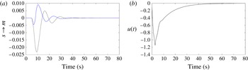
Figure 12(a) compares the controlled and uncontrolled response of
 $m(t)$
to an impulse in
 $s(t)$
. Figure 12(b) shows the corresponding non-dimensional control law. These figures show that while complete fluctuation negation is impossible, fluctuation damping is achievable. Such a control law will negate a portion of upstream disturbances. Furthermore since part of the perturbation will not have the chance to be further amplified in the shear layer this should result in noteworthy reduction in downstream TKE fluctuations. Hervé et al. (Reference Hervé, Sipp, Schmid and Samuelides2012) found a far greater reduction for the impulse responses. One of the reasons for this is the location of the actuator, at the wall in our experiment, instead of in the bulk above the wall in the numerical simulation. The vortices created by the obstacle travel too far from the wall (approximately one step height) to be as successfully suppressed.
(a) Controlled (grey) and uncontrolled (black) response to an impulse in
 $s(t)$
. (b) Resulting control law
 $u(t)$
.

4.2. Control results
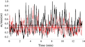
Figure 13 shows a comparison between outputs for the controlled and uncontrolled flow. Comparison was done over 14 min (21 000 iterations). The results clearly show a reduction in fluctuations for the controlled flow (
 $-35\,\%$
). Moreover a reduction in mean value is also observed (
 $-15\,\%$
). The mean value reduction is an added benefit of fluctuation reduction. Better performance could be expected when considering the impulse responses. Additional noise sources not accounted for by the upstream sensor are likely to be present in an experimental flow, contributing to degraded performance.
Controlled (grey) and uncontrolled flow (black) outputs. Mean values are also displayed.

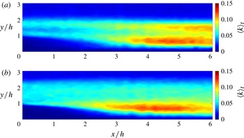
Comparison of the time-averaged two-dimensional TKE field obtained for the perturbed, uncontrolled (a) and controlled (b) flows.

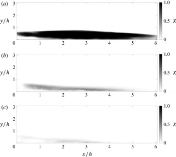
Ratio of negative to positive longitudinal velocity
 ${\it\chi}$
for the unperturbed (a), perturbed (b) and controlled (c) flows.

Figure 14 shows the mean TKE field for the controlled and uncontrolled flows in the region of interest. The reduction in mean TKE is clear, as is a slight augmentation in recirculation size. Furthermore the effects of control are heterogeneous: while the TKE in the recirculation region seems mainly unaffected, the region of high TKE induced by the obstacle is successfully suppressed.
Figure 15 shows the ratio of negative to positive longitudinal velocity (
 ${\it\chi}$
) for the perturbed unperturbed (a), perturbed (b) and controlled (c) flows. This is an effective measure measure of recirculation. This result highlights the effect of the control action on recirculation.
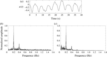
(a) Control law output
 $u(t)$
over 1 min. (b) Normalized frequency spectrum for
 $s(t)$
. (c) Normalized frequency spectrum for
 $u(t)$
.

Figure 16(a) shows the non-dimensional control output sampled over 1 min. One can see that the control signal is one of periodic suction. Figure 16(b,c) shows the frequency spectra for
 $s(t)$
and
 $u(t)$
. A double peak is present in both spectra for the same frequency. This explains the physical processes involved during control. An incoming vortex is detected as a spike in
 $s(t)$
. The response is a sharp aspiration as shown by figure 12. Thus, the control is operating in opposition.
5. Conclusion
For the first time, an experimental implementation of a feed-forward control algorithm based on an ARMAX model has been conducted on a BFS flow. Results show the validity of such an approach. Nevertheless, to ensure successful implementation special care should be given to actuation, in particular to prevent contamination of the upstream sensor. Moreover, this approach is limited to the linear regime of the flow.
Analysing impulse responses gives valuable insight into the flow controllability as well as the potential for success of the method. While these responses tell us that full negation of upstream disturbances is impossible, the computed model was able to reliably predict flow responses and yield a control law able to reduce energy levels and fluctuations. Future work should involve spanwise sensors and actuators thus allowing spanwise heterogeneous disturbances to be controlled as proposed and evaluated numerically by Semeraro et al. (Reference Semeraro, Bagheri, Brandt and Henningson2011).
Acknowledgement
The authors gratefully acknowledge the support of the DGA (Direction Générale de l’Armement).