








1 Introduction
Let k be a field. For
$x \in k$
 , we will denote

and for any set of polynomials
$\mathcal {P} \subset k[X_1,\ldots ,X_N]$
 we will call an element of
$\{0,1\}^{\mathcal {P}}$
 a zero-nonzero pattern on
$\mathcal {P}$
 .
If k is an ordered field we will denote for
$x \in k$
 ,

and for any set of polynomials
$\mathcal {P} \subset k[X_1,\ldots ,X_N]$
 we will call an element of
$\{0,1,-1\}^{\mathcal {P}}$
 a sign condition on
$\mathcal {P}$
 .
For any finite set
$\mathcal {P}$
 of polynomials in
$k[X_1,\ldots ,X_N]$
 ,
$V\subset k^N$
 , and
$\pi \in \{0,1\}^{\mathcal {P}}$
 , we denote by

In the case k is an ordered field,
$S \subset k^N$
 , and
$\sigma \in \{0,1,-1\}^{\mathcal {P}}$
 , we denote by

1.1 Background and prior work
Bounds on the number (or other topological invariants of the realizations like the number of connected components, etc.) of realizable zero-nonzero patterns or sign conditions of finite sets of polynomials have had many important applications in mathematics and theoretical computer science. To pick a few notable ones: they play a key role in bounding the number of point configurations as well as combinatorial types of polytopes in
$\mathbb {R}^d$
 [Reference Goodman and Pollack17], in bounding the number of geometric permutations induced by transversals to convex subsets of
$\mathbb {R}^d$
 [Reference Goodman, Pollack and Wenger18], bounding the number (also called the speed) of algebraically defined classes of graphs [Reference Alon, Pach, Pinchasi, Radoičić and Sharir2, Reference Sauermann34], in recent applications of the polynomial method to incidence combinatorics [Reference Basu and Sombra8, Reference Walsh41, Reference Walsh42, Reference Tao39, Reference Sheffer37, Reference Guth19], in proving lower bounds for testing membership in semi-algebraic sets using algebraic computation trees [Reference Ben-Or10, Reference Yao45, Reference Gabrielov and Vorobjov16], in proving lower bounds on projective dimensions of graphs and span programs [Reference Rónyai, Babai and Ganapathy32], bounding the
${\varepsilon }$
 -entropy of and volumes of tubes around algebraic varieties [Reference Basu and Lerario7, Reference Zhang and Kileel46], and a host of other applications (including some new ones introduced in this paper). The following two results may be considered as starting points.
Theorem A [Reference Rónyai, Babai and Ganapathy32, Reference Jeronimo and Sabia21].
Let k be a field and
$\mathcal {P} \subset k[X_1,\ldots ,X_N]_{\leq d}$
 be a finite set of polynomials of degree at most d. Then, the number of realizable zero-nonzero patterns on
$\mathcal {P}$
 (i.e., elements of
$\{0,1\}^{\mathcal {P}}$
 ) is bounded by
$(O(s d))^N$
 , where
$s = \mathrm {card}(\mathcal {P})$
 . (We say a zero-nonzero pattern
$\pi \in \{0,1\}^{\mathcal {P}}$
 is realizable if there exists
$x \in k^N$
 , such that
$\mathrm {sgn}(P(x)) = \pi (P)$
 for all
$P \in \mathcal {P}$
 .)
Theorem B [Reference Warren43].
Let k be an ordered field and
$\mathcal {P} \subset k[X_1,\ldots ,X_N]_{\leq d}$
 be a finite set of polynomials of degree at most d. Then, the number of realizable sign conditions on
$\mathcal {P}$
 is bounded by
$(O(s d))^N$
 , where
$s = \mathrm {card}(\mathcal {P})$
 . (We say a sign condition
$\sigma \in \{0,1,-1\}^{\mathcal {P}}$
 is realizable if there exists
$x \in k^N$
 , such that
$\mathrm {sign}(P(x)) = \sigma (P)$
 for all
$P \in \mathcal {P}$
 .)
The above theorems have been generalized in many different directions. For example, if
$k = \mathrm {R}$
 is a real closed field (e.g., the field
$\mathbb {R}$
 of real numbers), it is possible to obtain bounds on the higher Betti numbers of the realizations of sign conditions (see Theorem C below). Motivated by applications in discrete geometry (bounding the number of geometric permutations, as well as incidences), there was a need for more precise bounds on the number of realizable sign conditions: for example, upper bounds on the number of realizable sign conditions or even on the number of different connected components of the realizations restricted to an algebraic subset of the ambient space which may be of much smaller dimension (see, e.g., [Reference Goodman, Pollack and Wenger18] for one such application where the dimension of the algebraic subset plays a key role).
Before proceeding further, we recall some definitions from algebraic geometry and introduce some useful notations.
1.2 Basic definitions and notation
Let k denote an algebraically closed field. An algebraic subset V of
$k^N$
 Footnote 1 is the set of common zeros of a set of polynomials in
$k[X_1,\ldots ,X_N]$
 .
An algebraic subset admits a decomposition (in the Zariski topology) into a finite union of irreducible ones which are called varieties. The dimension of a variety V, denoted
$\dim V$
 , is the Krull dimension of its coordinate ring
$k[V] = k[X_1,\ldots ,X_n]/I(V)$
 , where
$I(V)$
 is the defining ideal of V, that is,
$I(V) = \{f \in k[X_1,\ldots ,X_N] \;\mid \; f(x) = 0, x \in V \}$
 . The degree of V, denoted
$\deg V$
 , is equal to the number of points in the intersection
$V \cap L$
 for a generically chosen affine subspace L of dimension
$N-\dim V$
 in
$k^N$
 .
Finally, we define the degree,
$\deg (V)$
 , of an algebraic set V to be the sum of the degrees of its irreducible components, and the dimension,
$\dim (V)$
 , of V to be the maximum of the dimensions of its irreducible components.
A subset
$S \subset k^N$
 is called a constructible subset if it is defined by a Boolean formula with atoms of the form
$P = 0$
 for
$P \in k[X_1,\ldots ,X_N]$
 . A subset
$S \subset \mathbb {P}_k^N$
 is called a constructible subset if it is defined by a Boolean formula with atoms of the form
$P = 0$
 for
$P \in k[X_0,X_1,\ldots ,X_N]$
 , with P homogeneous.
If
$\mathrm {R}$
 is a real closed field (e.g.,
$\mathbb {R}$
 ), a subset
$S \subset \mathrm {R}^N$
 is called a semi-algebraic subset if it is defined by a Boolean formula with atoms of the form
$P = 0, P> 0$
 for
$P \in \mathrm {R}[X_1,\ldots ,X_N]$
 . We call a subset of
$\mathbb {A}_{\mathrm {R}}^N$
 or
$\mathbb {P}_{\mathrm {R}}^N$
 to be
$\mathcal {P}$
 -semi-algebraic, for a finite set of polynomials
$\mathcal {P}$
 , if every P in the Boolean formula defining the set belongs to
$\mathcal {P}$
 .
If
$\mathrm {C} = \mathrm {R}[i]$
 (which is the algebraic closure of
$\mathrm {R}$
 ), then a constructible subset of
$\mathrm {C}^N$
 is also a semi-algebraic subset of
$\mathrm {R}^{2N} = \mathrm {C}^N$
 .
Notation 1.1. In case
$k = \mathrm {C} = \mathrm {R}[i]$
 , where
$\mathrm {R}$
 is a real closed field, for any locally closed semi-algebraic set S we denote by

where
$\mathrm {H}_i(S,\mathbb {Z}/2\mathbb {Z})$
 denotes the i-th homology group of S with coefficients in
$\mathbb {Z}/2\mathbb {Z}$
 (see, e.g., [Reference Basu, Pollack and Roy5, Chapter 6, Section 3]) and call
$b_i(S)$
 the i-th Betti number of S (with coefficients in
$\mathbb {Z}/2\mathbb {Z}$
 ).
Note that
$b_0(S)$
 is just the number of semi-algebraically connected components of S.Footnote 2
We can now state several generalizations of the two basic theorems mentioned before. The following theorem extends Theorem B in several directions.
Theorem C [Reference Basu, Pollack and Roy4].
Let
$\mathrm {R}$
 be a real closed field and
$V \subset \mathrm {R}^N$
 be an algebraic subset defined by polynomials of degrees bounded by d with
$\dim _{\mathrm {R}} V = p$
 , and
$\mathcal {P} \subset \mathrm {R}[X_1,\ldots ,X_N]_{\leq d}$
 . Then, for each
$i, 0 \leq i \leq p$
 , the sum of the i-th Betti numbers of the realizations in V of all sign conditions on
$\mathcal {P}$
 is bounded by

where
$s = \mathrm {card}(\mathcal {P})$
 .
However, the above result is still insufficient for certain modern applications involving applications of the polynomial partitioning technique, where one needs more refined results where the dependence of the bound on the degree of the variety V and the degrees of the polynomials in
$\mathcal {P}$
 is separated out.
Suppose that we have a sequence of algebraic sets
$V_0,\ldots ,V_\ell \subset \mathrm {R}^N$
 cut out by a sequence of real polynomials of degrees
$d_1,d_2, \ldots ,d_\ell $
 , with real dimensions
$p_1 \geq p_2 \geq \cdots \geq p_\ell $
 , and the degrees of the polynomials in
$\mathcal {P}$
 are bounded by
$d \geq d_\ell $
 .
The following result in this direction is proved in [Reference Barone and Basu3] and has been applied in the context of incidence geometry [Reference Basu and Sombra8, Reference Walsh41, Reference Walsh42].
Theorem D [Reference Barone and Basu3, Theorem 4].
Suppose that

and
$d_\ell \leq \frac {1}{N+1} d$
 . Then, the number of semi-algebraically connected components of the realizations of all sign conditions on
$\mathcal {P}$
 restricted to
$V = V_\ell $
 is bounded by

The following related result, which has applications in incidence geometry via the polynomial partitioning technique (see, e.g., [Reference Guth19, Reference Sheffer37]), was obtained by M. Walsh [Reference Walsh42]. We denote by
$\mathrm { Z}(P,V)$
 the set of zeros of a polynomial restricted to a set V. If
$V = \mathrm {R}^N,\mathrm {C}^N$
 , we will sometimes omit V and denote
$\mathrm {Z}(P) = \mathrm {Z}(P,V)$
 .
Theorem E [Reference Walsh42, Theorem 2.12].
Let
$\mathrm {R}$
 be a real closed field,
$\mathrm {C} = \mathrm {R}[i]$
 the algebraic closure of
$\mathrm {R}$
 , and
$V \subset \mathrm {C}^N$
 be an algebraic variety with
$\dim V = p$
 , and
$P \in \mathrm {R}[X_1,\ldots ,X_n]$
 . Then, the number of semi-algebraically connected components C of
$\mathrm {R}^N - \mathrm {Z}(P,\mathrm {R}^N))$
 such that
$C \cap V(\mathrm {R}) \neq \emptyset $
 is bounded by
$ C(N) \cdot \deg (V) \cdot \deg (P)^p$
 where the constant
$C(N)$
 depends on N (in an unspecified way), and
$V(\mathrm {R})$
 denotes the
$\mathrm {R}$
 -points of V.
Remark 1.2. Note that the quantity being bounded in Theorem E is a priori smaller than the number of semi-algebraically connected components of
$V(\mathrm {R}) - \mathrm {Z}(P,\mathrm {R}^N)$
 . In particular, one cannot derive any useful bound on the number of semi-algebraically connected components of
$V(\mathrm {R})$
 itself from Theorem E (by letting P be a nonzero constant polynomial).
Remark 1.3. Notice also that while Theorem C has better dependence in the combinatorial part (the part depending on s) on the dimension of the variety V, the algebraic part (the part depending on the degree) is oblivious of the dimension of the variety and depends exponentially on N, the dimension of the ambient space. The bounds in Theorems D and E are better, but they still depend on N (through the quantity
$C = C(N)$
 , presumably exponential, in the case of Theorem E).
In many applications, the dimension of V may be much smaller than N. For instance, consider the Plücker embedding of the Grassmannian variety
$\mathrm {Gr}(m,M)$
 of m-dimensional subspaces in
$k^{M}$
 in the
$\binom {M}{m} -1$
 -dimensional projective space. It is well known that
$\dim \mathrm {Gr}(m,M) = m(M-m)$
 . Thus, if
$m = \lceil M/2 \rceil $
 , while the dimension of the variety
$V = \mathrm {Gr}(m,M)$
 is polynomial in M, the dimension N of the ambient projective space is exponentially large in M. In such a situation, the bounds in Theorems D and E, which have exponential dependence on N, would produce a bound doubly exponential in M.
Laszlo and Viterbo [Reference Laszlo and Viterbo28] proved the following:
Theorem F [Reference Laszlo and Viterbo28, Theorem 1.2].
The sum of all
$\mathbb {Z}/2\mathbb {Z}$
 -Betti numbers of
$V(\mathrm {R})$
 , where V is a nonsingular real variety of degree D and dimension p, is bounded by

Remark 1.4. The proof of Theorem F relies on sophisticated calculation of characteristic classes of the underlying smooth manifold of V and hence cannot be applied to singular varieties.
Remark 1.5. The bound in Theorem F in particular gives a bound on the number of semi-algebraically connected components of V which just depends on the degree of V and is independent of the dimension of the ambient space and is closest in spirit to the results in this paper. This bound was further improved to
$D^{p+1}$
 in [Reference Kharlamov23]. However, these bounds only apply to nonsingular real projective varieties – while in the results about sign conditions proved in this paper (see Theorem 2.5 and Remark 2.6 below) the hypothesis on V is much weaker – namely that V only needs to be a union of affine varieties
$V_i$
 , such that each
$V_i$
 has the same real dimension at all points of
$V_i(\mathrm {R})$
 . Many naturally occurring real varieties, such as Schubert subvarieties of flag varieties, rank subvarieties in spaces of matrices, as well as other determinantal varieties (see [Reference Manivel30] for definitions), are often singular but satisfy the real equidimensionality condition mentioned above.
1.3 Summary of main contributions
In this paper we consider varieties and polynomials over real and complex numbers (in fact more generally over arbitrary real closed and algebraically closed fields). We prove bounds on the number of realizable zero-nonzero patterns and sign conditions (and also on the number of connected components of their realizations which is a priori bigger number) which are independent of N and depend only on the number and degrees of the polynomials, and the degree (of the embedding of V in
$\mathbb {A}_k^N$
 or in
$\mathbb {P}_k^N$
 ) and the dimension of V. These appear as Theorems 2.1, 2.5, 2.12, 2.14, and 2.17 in Section 2 below.
The independence of these bounds from the dimension N of the ambient space is a new feature of these bounds (see Remark 2.10 about the existence of such bounds). This feature is potentially useful in any application where one is interested in the number of zero-nonzero patterns (resp. sign conditions) restricted to algebraic subsets of dimension much smaller than that of the ambient dimension. We discuss examples of such applications below in Section 1.3.3.
1.3.1 Methods
Our techniques for dealing with zero-nonzero patterns and sign conditions are different. To prove the upper bound on the number of zero-nonzero patterns of a family of polynomials restricted to an algebraic subset V of
$\mathbb {A}_k^N$
 , we closely follow the proof given in [Reference Jeronimo and Sabia21, Reference Basu, Pollack and Roy6], with the modification that all algebraic subsets that are considered in the proof are contained in V and we can bound their degrees in terms of
$\deg V$
 and the degrees of the given polynomials. We prove an upper bound on the sum of the degrees of the Zariski closure of the realizations of all zero-nonzero patterns with nonempty realizations on V, which in turn gives an upper bound on the number of realized zero-nonzero patterns. An important role in the argument is played by the generalized Bezout inequality (Theorem H).
For the problem of bounding realizable sign conditions over ordered fields, we assume without loss of generality that the field
$k = \mathrm {R}$
 is a real closed field. The main technique that is used for proving bounds on the number of realizable sign conditions (or more generally bounding the Betti numbers of these realizations) is via a technique of infinitesimal perturbations (see, e.g., [Reference Basu, Pollack and Roy4, Reference Basu, Pollack and Roy5]). The idea is to perturb the given set of polynomials using infinitesimal elements in some real closed extension of
$\mathrm {R}$
 , so that:
-
A. The polynomials in the new set have the same degrees as the ones in the given set, but in addition have better algebraic properties – like being in general position. These algebraic properties help control the combinatorial part of the bound.
-
B. The realizations of the various realizable sign conditions are related to those of the given set in some way, so that bounding the number (or more generally the Betti numbers) of realizations of the sign conditions of the new set of polynomials suffices to bound the corresponding quantity for the original set.
-
C. Finally, the problem of bounding the number of realizable sign conditions (or more generally the Betti numbers of the realizations) can be reduced to bounding the corresponding quantity for all the nonempty algebraic subsets that one can define using the perturbed set of polynomials.
Our technique for proving upper bounds on the number of realizable sign conditions follows a similar paradigm but meets two important obstacles.
-
A. Since we are not given the polynomials that define V, we are not able to deform V infinitesimally maintaining its degree;
-
B. as a result, while we are able to reduce, using usual techniques, to the case of bounding the number of semi-algebraically connected components of certain algebraic subsets of $V(\mathrm {R})$
 , all existing bounds for bounding the number of semi-algebraically connected components of possibly singular real algebraic sets depend exponentially on the dimension of the ambient space.

We overcome these problems by first reducing the problem to the problem of bounding the number of semi-algebraically connected components of an appropriate number of real algebraic subsets
$X(\mathrm {R}) \subset V(\mathrm {R})$
 , of codimension one in V, then, after taking the image under a generic projection
$\pi $
 to
$\mathrm {R}^p$
 (where
$p= \dim V$
 ), to the problem of bounding the number of semi-algebraically connected components of the semi-algebraic set consisting of the
$\mathrm {R}$
 -points of
$\pi (X) - \mathrm {Sing}(\pi (X))$
 . We can use the classical bound due to Oleı̆nik and Petrovskiı̆ [Reference Petrovskiĭ and Oleĭnik31] to bound the latter quantity. This bound depends exponentially on the dimension of the ambient space, but since this is p in this situation, we can tolerate the exponential dependence on p. The technique described above for obtaining bounds on the number of semi-algebraically connected components of a real variety only in terms of its degree is new and, in our opinion, the most important technical contribution of the paper.
1.3.2 Tightness
Our bound (on the sum of the degrees of the realizations) in the algebraically closed case is tight (see Remark 2.2). In the real closed case, our main result applies to a certain slightly restricted class of algebraic subsets of
$\mathrm {R}^N$
 that includes most real algebraic sets that occur in practice. The bound is tight in this case as well up to a factor of
$O(1)^{\dim V}$
 (see Remark 2.7).
1.3.3 Applications
We give several applications of our results. Some of these results improve or generalize prior results, leveraging our new bounds. These include upper bounds on the
${\varepsilon }$
 -entropy of real varieties (Theorem 3.1), and lower bounds on the depths of algebraic computation trees testing membership in a semi-algebraic set (Theorem 3.5). In each of these cases, the new bounds depend only on the degree and dimension of the relevant algebraic subset and are independent of (or in the
${\varepsilon }$
 -entropy case very weakly dependent on) the ambient dimension.
We also introduce a notion of additive (resp. multiplicative) rank of elements of a vector space (resp. algebra) relative to some algebraic subset
$\Delta $
 (Definitions 5.1 and 5.9). This is motivated from quantum complexity theory, where
$\Delta $
 can be thought of as an algebraic family of allowed gates (i.e., a set of unitary operators operating on the Hilbert space associated to an n-qubit quantum register each having unit cost). We extend the definition of ranks to subsets of the vector space (resp. algebra), and prove lower bounds on the rank of subsets which have some structure (Theorems 5.4, 5.6, 5.12, and 5.13). As a consequence, finite subsets which are “grid”-like (i.e., have some algebraic structure) must contain elements of relatively large rank. As an application of the rank lower bound theorems, we show how to recover Shannon’s lower bound theorem for classical circuits in the case of quantum circuits with algebraic families of allowed gates (Theorems 5.21 and 5.28).
The rest of the paper is organized as follows. We state our mathematical results in the following Section 2. In Section 3 we describe some of the geometric applications of theorems stated in Section 2. These include:
-
A. bounding the ${\varepsilon }$
-entropy of real varieties (Section 3.1); -
B. an improvement of known lower bound results for algebraic computation trees (Section 3.2).

Section 4 is devoted to the proofs of all the results mentioned above.
In Section 5, we prove lower bounds on the relative ranks, additive as well as multiplicative in vector spaces and algebras, respectively, and over algebraically closed as well as real closed fields, and show that the lower bounds on ranks of subsets in an algebra imply lower bounds on quantum circuit complexity with algebraic families of allowed gates (Section 5.3).
Finally, in Section 6 we state some open problems for future research.
2 Upper bounds on zero-nonzero patterns and sign conditions
2.1 Bound on the number of realizable zero-nonzero patterns
We will denote

and call
$\Pi (\mathcal {P},V)$
 the set of realizable zero-nonzero patterns of
$\mathcal {P}$
 on V.
We are now in a position to state our first result.
Theorem 2.1. Let
$V \subset k^N$
 (resp.
$V \subset \mathbb {P}_k^n$
 ) be an algebraic subset with
$\deg V = D$
 ,
$\dim V = p$
 , and
$\mathcal {P} \subset k[X_1,\ldots ,X_N]_{\leq d}$
 (resp.
$\mathcal {P} \subset k[X_0,X_1,\ldots ,X_N]_{\leq d}$
 ) be a finite set of polynomials (resp. homogeneous polynomials), with
$\mathrm {card}(\mathcal {P}) = s$
 . Then,

(where
$\overline {({\mathcal R}(\pi ,V))}$
 denotes the Zariski-closure of
${\mathcal R}(\pi ,V)$
 ).
Remark 2.2 (Tightness).
The bound in (the second inequality of) Theorem 2.1 is tight. To see this, let
$N> 2p$
 , and V be a union of D disjoint affine subspaces of dimension p in
$k^N$
 . Let
$\mathcal {P} = \{P_1,\ldots ,P_s\} \subset k[X_1,\ldots ,X_N]$
 , where each
$P_i = \prod _{j=1}^{d} L_{i,j}$
 , with
$L_{i,j} \in k[X_1,\ldots ,X_N], \deg (L_{i,j}) =1$
 . Also suppose that the polynomials
$L_{i,j}$
 are generic (of degree
$1$
 ). It is easy to see that with these choices,

2.2 Bound on the number of realizable sign conditions
Now suppose
$\mathrm {R}$
 is a real closed field and let
$\mathrm {C} = \mathrm {R}[i]$
 . For an algebraic subset
$V \subset \mathrm {C}^N$
 , we denote by
$V(\mathrm {R}) = V \cap \mathrm {R}^N$
 the set of its real points. We say that V is a real algebraic set (or a real variety if V is irreducible), if V is closed under conjugation taking z to
$\bar {z}$
 . It is easy to see that a real algebraic set is the vanishing locus of a finite number of polynomials in
$\mathrm {R}[X_1,\ldots ,X_N]$
 .
For
$x \in V(\mathrm {R})$
 , we will denote by
$\dim _x V(\mathrm {R})$
 the local real dimension (see, e.g., [Reference Basu, Pollack and Roy5, page 191]) of
$V(\mathrm {R})$
 at x (as a semi-algebraic set). If V is a nonsingular variety of dimension p, then
$\dim _x V(\mathrm {R}) = p$
 for every
$x \in V(\mathrm {R})$
 .
We will denote

and call
$\Sigma (\mathcal {P},S)$
 the set of realizable sign conditions of
$\mathcal {P}$
 on S.
Notation 2.3. For S a semi-algebraic set, we will denote by
$\mathrm {Cc}(S)$
 the set of semi-algebraically connected components of S.
Remark 2.4. Note that
$\mathrm {card}(\mathrm {Cc}(S)) = b_0(S)$
 .
We can now state our main theorems on bounding the number of semi-algebraically connected components of the realizations of realizable sign conditions of a finite set of polynomials restricted to the real points of a given algebraic set V.
Theorem 2.5. Let
$V=V_1\cup \cdots \cup V_m\subset \mathrm {C}^N$
 be a union of real varieties. Set

and assume that

Let
$\mathcal P\subset \mathrm {R}[X_1,\ldots ,X_N]_{\le d}$
 be a finite set of polynomials, with
$\mathrm {card}(\mathcal P)=s$
 . Then

where

In particular,

(where the implied constant in the
$O(\cdot )$
 notation is an absolute constant).
Schematic for the example with
$p=1$
 and
$N=2$
 :
$V(\mathrm {R})$
 consists of
$D^2$
 disjoint ovals
$V_{i,j}$
 , and
$\mathrm {Z}(\mathcal P,\mathrm {R}^2)$
 is a collection of vertical lines
$X_1=\delta _{i,j}$
 intersecting each oval
$V_{0,j}$
 in
$2sd$
 points.

Remark 2.6. The hypothesis on V is clearly satisfied if each
$V_i$
 is nonsingular of dimension p (see also Remark 1.5).
Remark 2.7 (Tightness).
We give examples showing that the dependence on D and
$sd$
 in Theorem 2.5 is essentially sharp when
$p=1$
 , and discuss the situation for
$p>1$
 .
The case
$\mathbf {p=1, N=2}$
 Let
$V\subset \mathrm {C}^2$
 be the hypersurface defined by
$Q=0$
 , where

Then,
$\dim V=1$
 and
$\deg (V)=2D$
 . For all sufficiently small real
$\varepsilon>0$
 , the variety V is nonsingular and
$V(\mathrm {R})$
 consists of
$D^2$
 pairwise disjoint ovals

with
$(i,j)$
 contained in the bounded component of
$\mathrm {R}^2\setminus V_{i,j}$
 .
Let
$\mathcal P=\{P_1,\dots ,P_s\}$
 , where

Choose parameters satisfying

(where
$\ll $
 means “sufficiently small”). Then, for each i,
$\mathrm {Z}(P_i,\mathrm {R}^2)$
 is the union of d vertical lines, and each such line meets every oval
$V_{0,0},\dots ,V_{0,D-1}$
 in exactly two distinct points (see Figure 1). Consequently, the arrangement
$\mathrm {Z}(\mathcal P,\mathrm {R}^2)$
 meets each oval
$V_{0,j}$
 in
$2sd$
 distinct points, and hence cuts
$V_{0,j}$
 into
$2sd$
 disjoint arcs. Summing over
$j=0,\dots ,D-1$
 and accounting for the remaining ovals, one obtains

which matches the upper bound in Theorem 2.5 in the case
$p=1$
 .
The case
$\mathbf {p>1}$
 . For
$p>1$
 , the situation is more subtle. Let
$N=p+1$
 and take
$V\subset \mathrm {C}^N$
 to be the union of
-
• D real affine hyperplanes in $\mathrm {C}^N$
, together with -
• the hypersurface in $\mathrm {C}^N$
defined by $$\begin{align*}Q \;=\; \sum_{i=1}^{N}\ \prod_{j=0}^{D-1}(X_i-j)^2\;-\;\varepsilon, \qquad 0<\varepsilon\ll 1. \end{align*}$$


With this choice,
$V(\mathrm {R})$
 is the union of
$D^{p+1}$
 bounded semi-algebraically connected components coming from zeros of Q, as well as D hyperplanes. Moreover,
$\dim V = p$
 , and
$\deg (V) = D + 2 D = 3 D$
 .
Let
$\mathcal P=\mathcal P_1\cup \mathcal P_2\subset \mathrm {R}[X_1,\dots ,X_N]$
 , where
$\mathcal P_1$
 consists of s polynomials, each of which is a product of d distinct linear forms, and the resulting collection of
$sd$
 linear factors is chosen generically. Let
$\mathcal P_2=\{P_1,\dots ,P_s\}$
 with

for parameters satisfying

In this regime, one checks that the contribution from the hyperplane part of
$V(\mathrm {R})$
 and from the hypersurface part combine to give the lower bound

At present, we do not know an example that matches the upper bound in Theorem 2.5 for
$p>1$
 even up to a factor
$\Omega (1)^p$
 . Closing this gap remains an interesting open problem.
Theorem 2.5 may be interesting even in the case
$\mathcal {P} = \emptyset $
 . In this case, we just obtain a bound on the number of semi-algebraically connected components of V having the top real dimension. In order to state this formally, we introduce a new notation.
Notation 2.8. For any semi-algebraic set S and
$p \geq 0$
 , we denote

We have the following slight variant of Theorem 2.5 in the case of algebraic sets that will be useful later.
Theorem 2.9. Let
$V \subset \mathrm {C}^N$
 be a real algebraic set, with
$\deg (V) =D$
 , and
$\dim V = p$
 . Then,

In particular, if every semi-algebraically connected component of
$V(\mathrm {R})$
 has (real) dimension equal to p, then

Remark 2.10. Note that if
$V \subset \mathbb {P}_{\mathrm {C}}^N$
 is a variety with
$\dim V = p$
 , such that V is not contained in any hyperplane of
$\mathbb {P}_{\mathrm {C}}^N$
 , then
$N \leq \deg (V) + p - 1$
 (see, e.g., [Reference Beltrametti, Carletti, Gallarati and Bragadin9, Proposition 4.5.6]).Footnote 3 Now, suppose V is a real variety. Then, V can be cut out by real polynomials of degree at most D. Now using the basic inequality on the Betti numbers of real algebraic sets due to Oleı̆nik and Petrovskiı̆ [Reference Petrovskiĭ and Oleĭnik31] (see, e.g., [Reference Basu, Pollack and Roy5, Proposition 7.28]), we would obtain the bound:

Then for D large enough, the bound in inequality (2.3) is worse than the bound in Theorem 2.9. Similar remarks apply to Theorems 2.5, 2.12, and 2.19 as well.
Remark 2.11. As remarked earlier, many naturally occurring real varieties, such as Schubert subvarieties of flag varieties, rank subvarieties in spaces of matrices, as well as other determinantal varieties, are not nonsingular but satisfy the hypothesis of Theorem 2.5. These varieties in general will not satisfy the hypothesis of Theorem F because of the presence of singularities.
However, there exist real varieties for which the hypothesis of Theorem 2.5 is not satisfied.
-
A. The singular curve $V \subset \mathrm {C}^2$
in the plane defined by
$Y^2 = X^2(X-1)$
. In this case
$\dim V = 1$
, but
$V(\mathrm {R})$
contains the isolated point
$x = (0,0)$
, and
$\dim _x V(\mathrm {R}) = 0 < 1$
. Thus, V does not satisfy the hypothesis of Theorem 2.5. -
B. Another interesting example is the well-known Whitney umbrella, $V \subset \mathrm {C}^3$
, defined by the equation
$X^2 - Z Y^2 = 0$
. In this case
$V(\mathrm {R})$
has only one connected component, but every point
$x \in V(\mathrm {R})$
on the “stick” of the umbrella (namely the points satisfying
$Z < 0$
) has local dimension
$\dim _x V(\mathrm {R}) = 1 < 2 = \dim V$
. The real variety V does not satisfy the hypothesis of Theorem 2.5 (because of the lower-dimensional stick of the umbrella).


We also prove a projective version of Theorem 2.5. It is no longer meaningful to talk about the sign of a (homogeneous) polynomial in a real projective space. However, one still has the notion of zero-nonzero patterns. We bound the number of semi-algebraically connected components of the realizations on
$V(\mathrm {R})$
 of all zero-nonzero patterns of a finite set of homogeneous polynomials, where V is a nonsingular real projective variety.
Theorem 2.12 (Projective case).
Let
$V = V_1 \cup \cdots \cup V_m \subset \mathbb {P}_{\mathrm {C}}^N$
 be a union of real varieties, with
$\deg (V) = D$
 ,
$\dim V = p$
 , and such that for each
$i, 1 \leq i \leq m$
 , and
$x \in V_i(\mathrm {R})$
 ,
$\dim _x V_i(\mathrm {R}) = \dim V_i $
 , and let
$\mathcal {P} \subset \mathrm {R}[X_0,\ldots ,X_N]_{\leq d}$
 be a finite set of homogeneous polynomials, with
$\mathrm {card}(\mathcal {P}) = s$
 . Then,

Remark 2.13. Aside from the other applications that we discuss in the next section, Theorem 2.12 can be used to simplify proofs of certain quantitative results in discrete geometry. For example, in [Reference Goodman, Pollack and Wenger18], the authors prove a bound on the number of geometric permutations induced by k-dimensional transversals to a finite family of convex sets in
$\mathrm {R}^d$
 . A key role is played by a bound on the number of realizable sign conditions of a certain finite set of polynomials restricted to the Grassmannian
$\mathrm {Gr}(k,d)$
 (more accurately, the affine Grassmannian, but this is unimportant). In order to get a tight bound on this quantity that does not depend on the dimension of the Plücker embedding, the authors utilize a fact from real algebraic geometry – that the Grassmannian varieties
$\mathrm {Gr}(m,N)$
 can be embedded semi-algebraically (not scheme theoretically) as an algebraic subset of
$\mathrm {R}^{N^2}$
 [Reference Bochnak, Coste and Roy11, Theorem 3.4.4]. This last fact is somewhat remarkable as there is no such affine embedding of the complex Grassmannian (indeed the complex Grassmannian is compact as a topological space, while every complex affine algebraic set of positive dimension is necessarily noncompact). However, using Theorem 2.12 (noting that the Grassmannians are all nonsingular projective varieties) and the known expressions for the degree and the dimension of
$\mathrm {Gr}(m,N)$
 (see equation (3.2)), one can obtain a similar bound as in [Reference Goodman, Pollack and Wenger18, Theorem 2] without resorting to the clever nonstandard embedding of the real Grassmannian, and the new bound is a slight improvement over the original result when k is close to d.
The bound in Theorem 2.5 is worse than in Theorem 2.1 (in the dependence on D and d). We can prove a bound with a better dependence on D but with a more stringent assumption on V.
Theorem 2.14. Let
$\overline {V} \subset \mathbb {P}_{\mathrm {C}}^N$
 be a nonsingular complete intersection real variety with
$\deg \overline {V} = D$
 and
$\dim \overline {V} = p$
 . Let
$V = \overline {V} \cap \mathrm {C}^N$
 denote the corresponding affine variety.
Let
$\mathcal {P} \subset \mathrm {R}[X_1,\ldots ,X_N]_{\leq d}$
 be a finite set of polynomials with
$d \geq D$
 and
$\mathrm {card}(\mathcal {P}) = s$
 .
Then, for each
$i, 0 \leq i \leq p$
 ,

In particular,

(The constant in the
$O(1)$
 is absolute.)
Remark 2.15. Note that in Theorem 2.14 we can assume that V is contained in an affine subspace in
$\mathrm {C}^N$
 of dimension
$\leq p + \log _2 D$
 (see Lemma 4.23), and this removes the dependence on N from the final bound.
We are able to remove the nonsingularity restriction in Theorem 2.14. However, the bound that we prove is on an a priori smaller quantity which nevertheless arises in applications (see, e.g., Theorem E, which plays an important role in applications of the polynomial partitioning technique in problems of incidence geometry).
Notation 2.16. For
$S, V \subset \mathrm {R}^N$
 semi-algebraic subsets, we will denote

(Note that
$\mathrm {Cc}(S) = \mathrm {Cc}(S,\mathrm {R}^N)$
 .)
Theorem 2.17. Let
$V \subset \mathrm {C}^N$
 be a real complete intersection variety (not necessarily nonsingular) with
$\deg (V) = D$
 and
$\dim (V) = p$
 . Let
$\mathcal {P} \subset \mathrm {R}[X_1\ldots ,X_N]_{\leq d}$
 be a finite set of polynomials, with
$d \geq D$
 and
$\mathrm {card}(\mathcal {P}) = s$
 .
Then,

Remark 2.18. The exponent of D in the above bound comes from our proof technique which involves treating V as a real algebraic subset of
$\mathrm {R}^{2N}$
 by taking real and imaginary parts, that is, considering V as the real part of a complex complete intersection of degree
$D^2$
 .
We then use Theorem 2.14 which leads to an additional squaring. Improving this exponent will require some new idea.
2.3 Sum of Betti numbers of realizations of sign conditions
Using the result of Laszlo and Viterbo (Theorem F), we prove the following theorem, which extends Theorem C to the case when the ambient variety is more general than
$\mathrm {R}^N$
 .
Theorem 2.19. Let
$\overline {V} \subset \mathbb {P}_{\mathrm {C}}^N$
 be a nonsingular real variety with
$\deg V = D$
 and
$\dim V = p$
 . Let
$V = \overline {V} \cap \mathrm {C}^N$
 denote the corresponding affine variety. Let
$\mathcal {P} \subset \mathrm {R}[X_1,\ldots ,X_N]_{\leq d}$
 be a finite set of polynomials. Then, for each
$i, 0 \leq i \leq p$
 ,

3 Applications
3.1 Bound on the
${\varepsilon }$
-entropy of real varieties

In this section we assume that
$\mathrm {R} = \mathbb {R}$
 .
A quantitative result from real (or more accurately metric) algebraic geometry that is now of great interest in applications (in problems originating in machine learning) is a tight upper bound on the volume of an
${\varepsilon }$
 -tube around a real algebraic variety V intersected with a ball of a given radius. A recent result in this direction is [Reference Basu and Lerario7, Theorem 1.1], which gives a tight upper bound on this volume depending on the degree d of the polynomials defining V and the codimension of V.
More recently, using very different techniques (originally due to Vitushkin [Reference Vitushkin40]), Zhang and Kileel [Reference Zhang and Kileel46] proved another bound on the volume of such tubes, which matches the bound in [Reference Basu and Lerario7] in the regime of large N and fixed d. They applied their results to prove new bounds in approximation properties of low-rank tensors, on the required dimension for randomized sketching algorithms, and generalization error bounds for deep neural networks with rational or ReLU activation functions. Their technique depends crucially on a bound on the number of connected components of real algebraic varieties, and any improvement on this bound will automatically improve the bound in their paper. In particular, inequality (2.2) is applicable in their context.
We follow the same notation as in [Reference Zhang and Kileel46]. Let
$V(\mathrm {R}) \subset \mathbb {R}^N$
 be a real variety, and for
${\varepsilon }>0$
 denote by
$\mathcal {N}(V(\mathrm {R}),{\varepsilon })$
 the minimum number of
${\varepsilon }$
 -balls required to cover
$V(\mathrm {R}) \cap B_N(0,1)$
 . The quantity
$\log \mathcal {N}(V(\mathrm {R}),{\varepsilon })$
 is referred to as the
${\varepsilon }$
 -entropy of
$V(\mathrm {R}) \cap B_N(0,1)$
 , and an upper bound on
$\mathcal {N}(V(\mathrm {R}),{\varepsilon })$
 implies an upper bound on the volume of the
${\varepsilon }$
 -tube around
$V(\mathrm {R}) \cap B_N(0,1)$
 .
The following result appears in [Reference Zhang and Kileel46, page 2722, Table 1, entry on real varieties].
Theorem G. Let
$V(\mathrm {R}) \subset B_N(0,1)$
 be a real variety defined by polynomials of degrees at most d and
$\dim V = p$
 . Then,

We prove the following theorem.
Theorem 3.1. Let
$V \subset \mathrm {C}^N$
 be a real variety with
$\deg (V) = D, \dim V = p$
 , such that
$V(\mathrm {R}) \subset B_N(0,1)$
 . Then,

(see Notation 2.8).
In particular, if every point of
$V(\mathrm {R})$
 has local real dimension equal to p, then

Remark 3.2. Note that the right-hand side of the inequality in Theorem 3.1 depends very weakly on the embedding dimension N (
$\log N$
 instead of N) compared to the bound in Theorem G. Notice also that while the bound in Theorem G is in terms of the degrees of the real polynomials cutting out V, the bound in Theorem 3.1 is in terms of the degree of V (as a complex variety), which is a more intrinsic invariant. It is well known that any affine variety of degree D in
$\mathrm {C}^N$
 can be cut out by at most
$N+1$
 polynomials of degree at most D. However, if we use this fact in conjunction with Theorem G, we will end up with a much weaker bound than the one in Theorem 3.1 (N instead of
$\log N$
 in the expression on the right-hand side).

3.2 Lower bounds for algebraic computation trees
We briefly recall the definition of an algebraic computation tree (see, e.g., [Reference Gabrielov and Vorobjov16] from which the following description is taken).
Definition 3.4. An algebraic computation tree T with input variables
$X_1,\ldots ,X_N$
 is a tree having three kinds of vertices:
-
A. computation vertices having outdegree $1$
; -
B. branch vertices with outdegree $3$
, and the three outgoing edges labeled by
$0$
,
$1$
, and
$-1$
; -
C. leaves with outdegree $0$
and labeled by “YES” or “NO”.


There is a variable
$Y_v$
 attached to each vertex v of T. Moreover, an expression
$Y_v = a * b$
 , where
$* \in \{+,-,\times \}$
 is associated with each computation vertex v, and
$a,b$
 are either real constants, or input variables, or variables associated with predecessor vertices of v, or a combination of these.
At each branch vertex v, the variable
$Y_v$
 is assigned the value which is either a real constant, or an input variable, or a variable associated with a predecessor vertex. The three outgoing edges of a branch vertex v labeled
$0$
 ,
$1$
 , or
$-1$
 then correspond to signs
$Y_v = 0$
 ,
$Y_v> 0$
 ,
$Y_v <0$
 (respectively).
With each leaf w, we associate naturally a basic semi-algebraic set
$S_w \subset \mathbb {R}^N$
 , defined by a conjunction of inequalities of the type
$Y_v> 0$
 ,
$Y_v = 0$
 ,
$Y_v <0$
 , where v varies over all branch nodes on the path from the root to the leaf w and the sign of
$Y_v$
 corresponds to the sign of the branch taken by the path. The semi-algebraic set
$S_T$
 associated to the tree S is defined as the union

where
$\mathrm {Leaves}_1(T)$
 denotes the set of leaf nodes of T labeled “YES”.
We say that the algebraic computation tree T tests membership in the semi-algebraic set S. The height of a tree is the length of the longest path from its root to a leaf node.
The interpretation of this model of computation is as follows. On an input

the input variables
$X_i$
 get the corresponding values
$x_i$
 , the arithmetic operations are executed in computation vertices v, and
$Y_v$
 is assigned the corresponding real value.
At branch vertices, the outward branch is chosen corresponding to the assigned value of
$Y_v$
 . The input x belongs to the semi-algebraic set
$S_w$
 if this process ends in the leaf w. If w is a leaf marked “YES”, then x is said to be accepted by the tree T.
It was proved by Ben-Or [Reference Ben-Or10] that for any semi-algebraic set the height of an algebraic computation tree testing membership in a semi-algebraic set
$S \subset \mathrm {R}^N$
 is at least
$c_1 \log b_0(S) - c_2 N$
 , where
$c_1,c_2> 0$
 are absolute constants. Yao [Reference Yao45] proves that for any locally closed and bounded semi-algebraic set
$S \subset \mathrm {R}^N$
 , the height of any algebraic computation tree testing membership in S is bounded by

where
$b^{BM}(S)$
 denotes the Borel-Moore Betti numbers of S (they can also be defined as the dimensions of the compactly supported cohomology groups
$\mathrm {H}_c^*(S)$
 ). This result was extended recently by Gabrielov and Vorobjov [Reference Gabrielov and Vorobjov16] who proved that the height of an algebraic computation tree testing membership in a semi-algebraic set
$S \subset \mathrm {R}^N$
 (not necessarily locally closed) is at least

where
$c_1,c_2> 0$
 are absolute constants.
We prove the following theorem, which in particular improves the original result of Ben-Or in a direction that is independent of [Reference Yao45] and [Reference Gabrielov and Vorobjov16].
Theorem 3.5. Let
$S \subset \mathrm {R}^N$
 be a semi-algebraic set contained in a real algebraic set V. Suppose that V is a union of nonsingular real algebraic varieties, then the height of an algebraic computation tree testing membership in S is at least

where
$c_1, c_2> 0$
 are absolute constants.
Remark 3.6. Note that the above lower bounds are independent of the ambient dimension N. This is useful in situations where
$\dim V$
 and
$\log \deg V$
 are very small compared to the dimension of the ambient space.
Example 3.7. For example, consider the Grassmannian variety
$\mathrm {Gr}(m,N)$
 of m-dimensional subspaces in
$\mathrm {C}^N$
 , as a subvariety of
$\mathbb {P}_{\mathrm {C}}^{\binom {N}{m}-1}$
 . Let
$V = V_{m,N} \subset \mathrm {C}^{\binom {N}{m}}$
 be the affine cone over
$\mathrm {Gr}(m,N)$
 . Then, it is well known (see, e.g., [Reference Manivel30, Corollary 3.2.14]) that

where
$n = N - m$
 , while

This implies that
$\deg (V_{m,N}) = O(1)^{m(N-m)}$
 , and hence
$ \log (\deg (V_{m,N})) = O(m(N-m))$
 .
Now suppose that
$S \subset V_{m,N}(\mathrm {R})$
 is a semi-algebraic subset. Then, the lower bound in Theorem 3.5 yields that the depth of any algebraic computation tree testing membership in S is at least

while the result of Ben-Or implies a lower bound of

(with different constants
$c_1,c_2$
 ).
If
$m>2$
 and
$b_0(S) < \frac {c_2}{c_1}\binom {N}{m}$
 , then the last inequality will not give a nontrivial lower bound, while Theorem 3.5 will yield a nontrivial bound.
4 Proofs
4.1 Proof of Theorem 2.1
In our proof of Theorem 2.1, we will need to use the following generalized form of Bezout’s theorem (see for instance [Reference Fulton15, Example 8.4.6, page 148]).
Theorem H (Generalized Bezout).
Let
$V_1,\ldots ,V_s$
 be algebraic subsets of some projective space over k, such that each
$V_i$
 is a union of varieties of the same dimension, and
$Z_1,\ldots ,Z_t$
 be the irreducible components of the intersection
$V_1\cap \cdots \cap V_s$
 . Then

4.1.1 Outline of the proof of Theorem 2.1
The main idea (which is very similar to that used in [Reference Jeronimo and Sabia21], and also in [Reference Basu, Pollack and Roy6]) is to first bound the number of zero-nonzero patterns whose realizations are zero-dimensional using Theorem H. The main subtlety here is that the dimension of an algebraic set need not decrease upon intersection with another hypersurface. The problem of bounding the number of zero-nonzero patterns whose realizations have dimension
$>0$
 then can be reduced to the zero-dimensional case by taking generic hyperplane sections.
The proof of Theorem 2.1 will now follow from the following two lemmas. We follow closely the proof of Lemma 7.3 in [Reference Basu, Pollack and Roy6]. Observe that it is sufficient to prove the theorem in the case where V is irreducible of dimension p. Otherwise, we can take the irreducible decomposition of V, noting that their degrees add up to D.
Notation 4.1. For a finite set of polynomials
$\mathcal {Q} \subset k[X_1,\ldots ,X_N]$
 , and an algebraic set
$W \subset k^N$
 , we denote by
$\mathrm {Z}(\mathcal {Q},W)$
 the set of common zeros of
$\mathcal {Q}$
 in V. If
$\mathcal {Q} = \{Q\}$
 , we write
$\mathrm {Z}(Q,W)$
 for
$\mathrm {Z}(\mathcal {Q},W)$
 .
Let
$V,\mathcal {P}$
 be as in Theorem 2.1. For
$\rho \in \{0,1\}^{\mathcal {P}}$
 , let
${\mathcal P}_\rho = \{P \in {\mathcal P} \mid \rho (P) = 0\}$
 and let
$V_\rho = \mathrm {Z}({\mathcal P}_\rho ,V)$
 . Let
$V_\rho = V_{\rho ,1} \cup \cdots \cup V_{\rho ,n(\rho )}$
 denote the decomposition of
$V_\rho $
 into irreducible components.
We first prove a bound on the number of isolated points occurring as
${\mathcal R}(\rho ,V)$
 for some
$\rho \in \{0,1\}^{\mathcal {P}}$
 .
Lemma 4.2.

Proof. Let
${\mathcal P} = \{P_1,\ldots ,P_s\}$
 (the implicit ordering of the polynomials in
${\mathcal P}$
 will play a role in the proof).
First consider a sequence of p polynomials of
${\mathcal P}$
 ,
$P_{i_1},\ldots ,P_{i_p},$
 with
$1 \leq i_1 < \cdots < i_p \leq s$
 . Let
$\{W_{\alpha _1}\}_{\alpha _1 = 1,2..}$
 denote the irreducible components of
$\mathrm {Z}(P_{i_1},V)$
 . Similarly, let
$\{W_{\alpha _1,\alpha _2}\}_{\alpha _2 = 1,2,\ldots }$
 denote the irreducible components of
$W_{\alpha _1} \cap \mathrm {Z}(P_{i_2},V)$
 and so on. We prove by induction that for
$1 \leq \ell \leq p$


The claim is trivially true for
$\ell =1$
 . Suppose it is true up to
$\ell -1 $
 . Then, using Theorem H, we get that

Now suppose that
$\dim V_{\rho ,i} = 0$
 and let
$V_{\rho ,i} = \{x\}$
 .
We first claim that there must exist
$P_{i_1},\ldots ,P_{i_p} \in {\mathcal P}_{\rho }$
 , with
$1 \leq i_1 < i_2 < \cdots < i_p \leq s$
 , and irreducible affine algebraic varieties
$V_0, V_1,\ldots ,V_p$
 satisfying:
-
A. $V= V_0 \supset V_1 \supset V_2 \supset \cdots \supset V_p = \{x\}$
, and -
B. for each $j, \;1 \leq j \leq p$
,
$V_{j}$
is an irreducible component of
$\mathrm {Z}(P_{i_j},V_{j-1})$
which contains x.


Note that in the sequence,
$V_0,V_1,\ldots ,V_p$
 ,
$\dim (V_i)$
 is necessarily equal to
$p-i$
 . To prove the claim, let

with
$1 \leq j_1 < j_2 < \cdots < j_m \leq s$
 . Let
$W_0 = V$
 and for each
$h, 1 \leq h \leq m$
 , define inductively
$W_{h}$
 to be an irreducible component of
$\mathrm {Z}(P_{j_h},W_{h-1})$
 containing the point x. By definition,
$V = W_0 \supset W_1 \supset \cdots \supset W_m = \{x\}$
 and each
$W_h$
 is irreducible. Hence, there must exist precisely p indices,
$1 \leq \alpha _1 < \cdots < \alpha _p \leq m$
 such that
$\dim W_{\alpha _{i}} = \dim W_{\alpha _{i-1}} - 1$
 . If
$\beta \not \in \{\alpha _1,\ldots ,\alpha _p\}$
 , then
$W_{\beta } = W_{\beta - 1}$
 . Now, let
$i_1 = j_{\alpha _1},\ldots , i_p = j_{\alpha _p}$
 , and
$V_j = W_{\alpha _j}$
 for
$0 \leq j \leq p$
 . It is clear from construction that the sequence
$V_0,\ldots ,V_p$
 satisfies the properties stated above, thus proving the claim.
The number of sequences of polynomials of length p,
$P_{i_1},\ldots ,P_{i_p},$
 with
$1 \leq i_1 < \cdots < i_p \leq s$
 , is
$\binom {s}{p}$
 . The lemma now follows from the bound in (4.1).
The following lemma is a generalization of the above lemma to positive dimensions.
Lemma 4.3. For
$0 \leq \ell \leq p$


Proof. In order to bound the degree of
$V_{\rho ,i}$
 with
$\dim V_{\rho ,i} =\ell $
 , it suffices to count the isolated zeros of the intersection of
$V_{\rho ,i}$
 with a generic affine subspace L of dimension
$p-\ell $
 . Since there are only a finite number of
$V_{\rho ,i}$
 ’s to consider, we can assume that
-
A. L is generic for all of them,
-
B. the sets $V_{\rho ,i} \cap L$
are pairwise disjoint, -
C. for each $V_{\rho ,i}$
with
$\dim _{\mathrm {C}}V_{\rho ,i} =\ell $
,
$ \mathrm {Z}(P,L \cap V_{\rho ,i}) = \emptyset $
for each
$P \in {\mathcal P} \setminus {\mathcal P}_\rho $
.


Now, restrict to the subspace L and apply Lemma 4.2, noting that an isolated point of
$V_{\rho ,i} \cap L$
 is an isolated point of the family
${\mathcal P}$
 restricted to L.
4.2 Proofs of Theorems 2.5, 2.9, and 2.12
We first recall some preliminary definitions and results.
4.2.1 Multiplicity and singular points of a variety
Given a variety V and a point
$x \in V$
 , the multiplicity of V at x, denoted
$\mathrm {mult}_x(V)$
 , is defined as the degree of the exceptional divisor of the blow-up
$\widetilde {V}$
 of V at x [Reference Fulton15, Section 4.3, page 79]. This definition is equivalent to the definition of the Samuel multiplicity of the local ring
$\mathcal {O}_{V,x}$
 [Reference Fulton15, Example 4.3.1].
For an algebraic set V with irreducible components
$V_1,\ldots ,V_m$
 , and for
$x \in V$
 , we define
$\mathrm {mult}_x(V) = \sum _{i=1}^{m} \mathrm {mult}_x(V_i)$
 (where we define
$\mathrm {mult}_x(V_i) = 0$
 if
$x \not \in V_i$
 ).
Given a variety V, and a point
$x \in V$
 ,
$\mathrm {mult}_x(V) = 1$
 if and only if the local ring
$\mathcal {O}_{V,x}$
 is regular [Reference Fulton15, Example 4.3.5 (d)], and this is equivalent to V being nonsingular at x [Reference Fulton15, Section B.2.7, Page 429].
The following lemma follows immediately from the above which we record for future use.
Lemma 4.4. If V is an algebraic set, and
$x \in V$
 . Then, x is a nonsingular point of V if and only if
$\mathrm {mult}_x(V) = 1$
 .
The set of points of V which are not nonsingular will be denoted by
$\mathrm {Sing}(V)$
 . It is a proper closed subset of V (see [Reference Hartshorne20, Theorem 5.3]). If V is a variety, then
$\dim \mathrm {Sing}(V) < \dim V$
 .
We say that V is nonsingular if
$\mathrm {Sing}(V) = \emptyset $
 .
We also recall below the notion of an extension of a real closed field
$\mathrm {R}$
 by the real closed field
$\mathrm {R}{\langle }\zeta {\rangle }$
 of algebraic Puiseux series in
$\zeta $
 (where
$\zeta $
 is an infinitesimal, i.e.,
$\zeta $
 is positive but smaller than all positive elements of
$\mathrm {R}$
 ). These extensions are used for making infinitesimal perturbations of the given polynomials.
4.2.2 Real closed extensions and Puiseux series
We will need some properties of Puiseux series with coefficients in a real closed field. We refer the reader to [Reference Basu, Pollack and Roy5] for further details.
Notation 4.5. For
$\mathrm {R}$
 a real closed field, we denote by
$\mathrm {R} \left \langle {\varepsilon } \right \rangle $
 the real closed field of algebraic Puiseux series in
${\varepsilon }$
 with coefficients in
$\mathrm {R}$
 . We use the notation
$\mathrm {R} \left \langle {\varepsilon }_{1}, \ldots , {\varepsilon }_{m} \right \rangle $
 to denote the real closed field
$\mathrm {R} \left \langle {\varepsilon }_{1} \right \rangle \left \langle {\varepsilon }_{2} \right \rangle \cdots \left \langle {\varepsilon }_{m} \right \rangle $
 . Note that in the unique ordering of the field
$\mathrm {R} \left \langle {\varepsilon }_{1}, \ldots , {\varepsilon }_{m} \right \rangle $
 ,
$0< {\varepsilon }_{m} \ll {\varepsilon }_{m-1} \ll \cdots \ll {\varepsilon }_{1} \ll 1$
 .
Notation 4.6. For elements
$x \in \mathrm {R} \left \langle {\varepsilon } \right \rangle $
 which are bounded over
$\mathrm {R}$
 , we denote by
$\lim _{{\varepsilon }} x$
 the image in
$\mathrm {R}$
 under the usual map that sets
${\varepsilon }$
 to
$0$
 in the Puiseux series x.
Notation 4.7. If
$\mathrm {R}'$
 is a real closed extension of a real closed field
$\mathrm {R}$
 , and
$S \subset \mathrm {R}^{k}$
 is a semi-algebraic set defined by a first-order formula with coefficients in
$\mathrm {R}$
 , then we will denote by
$\mathrm {Ext}(S, \mathrm {R}') \subset \mathrm {R}^{\prime {k}}$
 the semi-algebraic subset of
$\mathrm {R}^{\prime {k}}$
 defined by the same formula. It is well known that
$\mathrm {Ext}(S, \mathrm {R}')$
 does not depend on the choice of the formula defining S [Reference Basu, Pollack and Roy5, Proposition 2.87].
4.2.3 Outline of the proof of Theorem 2.5
We first observe that it suffices to consider the case when V is irreducible of degree D and dimension p, satisfying that
$\dim _x V(\mathrm {R}) = p$
 for all
$x \in V(\mathrm {R})$
 . We introduce an infinitesimal
$\gamma _0$
 . Using the conic structure theorem for semi-algebraic sets [Reference Basu, Pollack and Roy5, Proposition 5.49], we are able to restrict attention to realizations of sign conditions which are contained in a ball of radius
$(1/\gamma _0)^{1/2}$
 . This necessitates the introduction of a new polynomial denoted by
$P_0$
 in the proof. We then define infinitesimal perturbations (using
$s+2$
 additional infinitesimals
$\gamma _1,\ldots ,\gamma _s,{\varepsilon },\delta $
 ) of the polynomials in
$\mathcal {P}$
 and prove that it suffices to bound the number of semi-algebraically connected components of the realizations on
$\widetilde {S} := \mathrm {Ext}(V(\mathrm {R}),\widetilde {\mathrm {R}})$
 (the extension of
$V(\mathrm {R})$
 to the field
$\widetilde {\mathrm {R}}$
 obtained from
$\mathrm {R}$
 by adjoining infinitesimal elements) of a certain set of weak sign conditions on this new set of
$4s+1$
 polynomials (Lemma 4.11). We then show that in order to bound these, it suffices to bound the number of semi-algebraically connected components of all the nonempty real algebraic sets defined by the perturbed set of
$4s +1$
 polynomials which are contained in
$\widetilde {S}$
 (Lemma 4.15).
If we consider the real algebraic set defined as the intersection of
$\widetilde {S}$
 with
$i, 0 \leq i \leq p$
 of the perturbed polynomials, then we get a real algebraic set of dimension
$p-i$
 and of degree bounded by
$D d^i$
 . So it now suffices to bound the number of semi-algebraically connected components of each of these real algebraic sets. Taking a sum of squares, we reduce to the case where the real algebraic set (say)
$\widetilde {Z}$
 is defined as the intersection of
$\widetilde {S}$
 with the
$\mathrm {Z}(\widetilde {Q}, \widetilde {\mathrm {R}}^N)$
 for a single polynomial
$\widetilde {Q}$
 .
We bound
$b_0(\widetilde {Z})$
 in two steps.
-
A. We first prove (using the semi-algebraic curve selection lemma and the intermediate value theorem for real closed fields) that
$$\begin{align*}b_0(\widetilde{Z}) \leq b_0(\mathrm{Z}(\widetilde{Q} - \zeta, \mathrm{Ext}(\widetilde{S},\widetilde{R}{\langle}\zeta{\rangle})) \end{align*}$$where $\zeta $
is a new infinitesimal (Lemma 4.16).
-
B. The real algebraic set
$$\begin{align*}\mathrm{Z}(\widetilde{Q} - \zeta, \mathrm{Ext}(\widetilde{S},\widetilde{R}{\langle}\zeta{\rangle}) \end{align*}$$if nonempty, is of dimension $p-1$
, satisfies the local dimension condition, and is of degree
$2 D d^i$
. If
$\pi $
denotes a generic projection to a real subspace of dimension p, then
$\pi (\mathrm {Z}(\widetilde {Q} - \zeta , \mathrm {Ext}(\widetilde {S},\widetilde {R}{\langle }\zeta {\rangle }))$
is a real hypersurface of degree
$2Dd^i$
and is defined by a real polynomial of that degree. Denoting
$\widetilde {Z} = \mathrm {Z}(\widetilde {Q} - \zeta , \mathrm {Ext}(\widetilde {S},\widetilde {R}{\langle }\zeta {\rangle }))$
we prove that
$b_0(\widetilde {Z})$
is bounded by
$b_0(\pi (\widetilde {Z}) - \mathrm {Sing}(\pi (\widetilde {Z})))$
(Lemma 4.19). Since
$\mathrm {Sing}(\pi (\widetilde {Z})))$
is a real algebraic subset of
$\pi (\widetilde {Z})$
, we can define its real points by taking the sum of squares of all partial derivatives of the polynomial defining
$\pi (\widetilde {Z})$
. We then use the Oleı̆nik-Petrovskiı̆ inequality [Reference Petrovskiĭ and Oleĭnik31] bounding the Betti numbers of real algebraic sets to bound the last quantity (Lemma 4.20).
-
C. We also need a bound on $b_0(V(\mathrm {R}))$
, since this term appears in the case
$i=0$
in the arguments described above.


Theorem 2.5 now reduces to bounding the contributions from the different algebraic sets mentioned above. We summarize this reduction step in Proposition 4.8 below.
4.2.4 Proof of Theorem 2.5
Let

We denote

where

and

For
$I \subset [1,s]$
 and
$\alpha \in \{\pm {\varepsilon }, \pm \delta \}^I$
 we denote

or

The following proposition is a key step in the proof of Theorem 2.5: it reduces the problem of bounding
$\sum _{\sigma \in \{0,1,-1\}^{\mathcal P}} b_0\big ({\mathcal R}(\sigma ,V(\mathrm {R}))\big )$
 to that of bounding the number of semi-algebraically connected components of certain auxiliary real algebraic sets constructed from
$\mathcal {P}$
 .
Proposition 4.8 (Master bound).
Let
$V\subset \mathrm {C}^N$
 be a real variety, with
$\dim V = p$
 . Let
$\mathcal P=\{P_1,\dots ,P_s\}\subset \mathrm {R}[X_1,\dots ,X_N]$
 , and let the notation
$\widetilde {\mathrm {R}}$
 ,
$P_0$
 ,
$Q_{I,\alpha }$
 , and
$Q_{I,\alpha ,0}$
 be as above. Let
$\zeta $
 be an infinitesimal over
$\widetilde {\mathrm {R}}$
 .
Define


Then

Theorem 2.5 will follow from Proposition 4.8 and bounds on A, B, and C appearing on the right-hand side of inequality (4.5) as given in the following two propositions.
Proposition 4.9 (Bound on C).
Let V be as in Proposition 4.8 with
$\deg (V) = D$
 , and such that for each
$x \in V(\mathrm {R})$
 ,
$\dim _x V(\mathrm {R}) = \dim V$
 . Then (following notation introduced in Proposition 4.8 (4.4))

Proposition 4.10 (Bounds on A and B).
Let V be as in Proposition 4.9, and
$\mathcal {P} \subset \mathrm {R}[X_1,\ldots ,X_N]_{\leq d}$
 . Suppose that
$\deg (V) = D$
 and
$\mathrm {card}(\mathcal {P}) = s$
 . Then (following notation introduced in Proposition 4.8 (4.2) and (4.3))

We now prove Propositions 4.8, 4.9, and 4.10.
We begin by proving Proposition 4.8. We will use the following lemmas.
Lemma 4.11. Let
$\sigma \in \Sigma (\mathcal {P},V(\mathrm {R}))$
 and
$C \in \mathrm {Cc}({\mathcal R}(\sigma ,V(\mathrm {R})))$
 . Then there exists a unique element
$\widetilde {C}_\sigma \in \mathrm {Cc}({\mathcal R}(\widetilde {\phi }_\sigma ,\mathrm {Ext}(V(\mathrm {R}),\widetilde {\mathrm {R}}))), $
 where

such that

Proof. Let
$x \in C$
 . Then,
$x \in {\mathcal R}(\widetilde {\phi }_\sigma ,\mathrm {Ext}(V(\mathrm {R}),\widetilde {\mathrm {R}}))$
 , and let
$\widetilde {C}_\sigma $
 be the semi-algebraically connected component of
${\mathcal R}(\widetilde {\phi }_\sigma ,\mathrm {Ext}(V(\mathrm {R}),\widetilde {\mathrm {R}}))$
 containing x. Then
$\widetilde {C}_\sigma \cap V(\mathrm {R}) = C \cap V(\mathrm {R})$
 (see [Reference Basu, Pollack and Roy5, Proposition 13.7]).
Lemma 4.12. For
$I \subset \{1,\ldots ,s\}$
 and
$\alpha \in \{\pm {\varepsilon }, \pm \delta \}^I$
 ,

Proof. Follows from the fact that
$\alpha (i)\gamma _i, i \in I$
 are independent transcendentals over
$\mathrm {C}$
 .
Remark 4.13. Note that as an immediate consequence of Lemma 4.12 we get that

whenever
$\mathrm {card}(I)> p$
 .
Lemma 4.14. Let
$V \subset \mathrm {R}^N$
 be a closed semi-algebraic set and
$\mathcal {Q} \subset \mathrm {R}[X_1,\ldots ,X_N]$
 a finite subset. Let
$C \in \mathrm {Cc}(S)$
 , where
$S \subset V$
 is the semi-algebraic set defined by

Then there exist a subset
$\mathcal {Q}' \subset \mathcal {Q}$
 and
$D \in \mathrm {Cc}(V \cap \mathrm {Z}(\mathcal {Q}',\mathrm {R}^N))$
 such that
$D \subset C$
 .
Proof. Let
$\mathcal {Q}'$
 be a maximal subset of
$\mathcal {Q}$
 with the property that
$\mathrm {Z}(\mathcal {Q}',\mathrm {R}^N) \cap C \neq \emptyset $
 . Then,
$\mathcal {Q}'$
 satisfies the required property in the lemma (see [Reference Basu, Pollack and Roy5, Proposition 13.1]).
Lemma 4.15. Let
$\sigma \in \{0,1,-1\}^{\mathcal {P}}$
 and
$C \in \mathrm {Cc}({\mathcal R}(\sigma ,V(\mathrm {R})))$
 . Then there exist
$I \subset \{1,\ldots ,s\}$
 ,
$\alpha \in \{\pm {\varepsilon },\pm \delta \}^I$
 , and D in the union of

and

such that

and

Lemma 4.16. Let
$S \subset \mathrm {R}^N$
 be a closed and bounded semi-algebraic set and
$Q \in \mathrm {R}[X_1,\ldots ,X_N]$
 , such that at every point
$x \in \mathrm {Z}(Q,S)$
 ,
$\dim _x \mathrm {Z}(Q,S) < \dim _x S$
 . Then,

In particular, if Q is nonnegative over S, then

Proof. Let
$\widetilde {S}$
 be the intersection of
$\mathrm {Ext}(S,\mathrm {R}{\langle }\zeta {\rangle })$
 with the set defined by
$-\zeta \leq Q \leq \zeta $
 . Let
$C \in \mathrm {Cc}(\mathrm {Z}(Q,S))$
 and
$x \in C$
 . Then, it follows from the hypothesis that
$\dim _x \mathrm {Z}(Q,C) < \dim _x S$
 . Hence, for all
$r>0$
 , denoting (here and elsewhere) by
$B_N(x,r)$
 the open Euclidean ball centered at x of radius r,
$\mathrm {Z}(Q,C) \cap B_N(x,r)$
 is nonempty and properly contained in
$S \cap B_N(x,r)$
 . So
$S - \mathrm {Z}(Q,C) \neq \emptyset $
 and
$x \in \overline {S - \mathrm {Z}(Q,C)}$
 . Applying the semi-algebraic curve selection lemma (see, e.g., [Reference Basu, Pollack and Roy5, Theorem 3.19]), there exists a semi-algebraic curve
$\gamma :[0,1] \rightarrow S$
 , such that
$\gamma (0) = x$
 , and
$\gamma ((0,1]) \subset S - \mathrm {Z}(Q,C)$
 . In particular,
$Q(\gamma (1)) \neq 0$
 .
Suppose without loss of generality that
$Q(\gamma (1))> 0$
 . Using the intermediate value property of the field
$\mathrm {R}{\langle }\zeta {\rangle }$
 ([Reference Basu, Pollack and Roy5, Proposition 4.3]), there exists
$\widetilde {t} \in \mathrm {R}{\langle }\zeta {\rangle }, \widetilde {t}> 0$
 , such that
$Q(\mathrm {Ext}(\gamma ,\mathrm {R}{\langle }\zeta {\rangle })(\widetilde {t})) = \zeta $
 , and let
$\widetilde {x} = \mathrm {Ext}(\gamma ,\mathrm {R}{\langle }\zeta {\rangle })(\widetilde {t})$
 . Then,
$\widetilde {x} \in \mathrm {Z}(Q-\zeta , \mathrm {Ext}(S,\mathrm {R}{\langle }\zeta {\rangle }))$
 . Let
$\widetilde {C} \in \mathrm {Cc}(\mathrm { Z}(Q-\zeta , \mathrm {Ext}(S,\mathrm {R}{\langle }\zeta {\rangle })))$
 with
$\widetilde {x} \in \widetilde {C}$
 . Then,
$\lim _\zeta \widetilde {C} \subset C$
 . Thus we have proved that for each
$C \in \mathrm {Cc}(\mathrm {Z}(Q,S))$
 , there exists
$\widetilde {C} \in \mathrm {Cc}(\mathrm {Z}(Q-\zeta , \mathrm {Ext}(S,\mathrm {R}{\langle }\zeta {\rangle }))) \cup \mathrm {Cc}(\mathrm { Z}(Q+\zeta , \mathrm {Ext}(S,\mathrm {R}{\langle }\zeta {\rangle })))$
 , with
$\lim _\zeta \widetilde {C} \subset C$
 . The lemma follows.
Remark 4.17. Note that the same conclusion in Lemma 4.16 holds for the number of bounded components when S is merely closed and not necessarily bounded.
Proof of Proposition 4.8.
Using Lemma 4.15, we are reduced to bounding the number of semi-algebraically connected components of the real algebraic sets,

and

where
$I \subset [1,s]$
 and
$\alpha $
 is as defined in Lemma 4.15. Using Lemma 4.12 and Remark 4.13, we only need to consider I with
$\mathrm {card}(I) \leq p$
 for the algebraic sets
$\bigcap _{i\in I} \mathrm {Z}(P_i + \alpha (i)\gamma _i,\mathrm {Ext}(V(\mathrm {R}),\widetilde {\mathrm {R}}))$
 and of cardinality at most
$p-1$
 for the algebraic sets
$\mathrm {Z}(P_0 - {\varepsilon } \gamma _0,\mathrm {Ext}(V(\mathrm {R}),\widetilde {\mathrm {R}})) \cap \bigcap _{i\in I} \mathrm {Z}(P_i + \alpha (i)\gamma _i,\mathrm {Ext}(V(\mathrm {R}),\widetilde {\mathrm {R}}))$
 .
Thus in order to bound
$\sum _{\sigma \in \{0,1,-1\}^{\mathcal {P}}} b_0({\mathcal R}(\sigma ,V(\mathrm {R})))$
 it suffices to bound (using Lemma 4.16 and Remark 4.17)
-
A. $b_0(\mathrm {Z}(Q_{I,\alpha } - \zeta , \mathrm {Ext}(V,\widetilde {\mathrm {R}}{\langle }\zeta {\rangle })))$
,
$I \subset [1,s], 1 \leq \mathrm {card}(I) \leq p$
, -
B. $b_0(\mathrm {Z}(Q_{I,\alpha ,0} - \zeta , \mathrm {Ext}(V,\widetilde {\mathrm {R}}{\langle }\zeta {\rangle })))$
,
$I \subset [1,s], 1 \leq \mathrm {card}(I) < p$
, and -
C. $b_0(V(\mathrm {R}))$
.


Item (A) corresponds to A, item (B) to B, and item (C) to C in the right-hand side of inequality (4.5).
We now prove Propositions 4.9 and 4.10.
Lemma 4.18. Let
$V \subset \mathrm {C}^N$
 be a variety with
$\dim V = p$
 . Then for all generically chosen linear maps
$\pi :\mathrm {C}^N \rightarrow \mathrm {C}^{p+1}$
 , the set of points
$w \in W = \pi (V)$
 such that
$\mathrm {card}(\pi ^{-1}(w) \cap V)=1$
 is Zariski dense in W.
Proof. It follows from the Noether normalization theorem (see, e.g., [Reference de Jong and Pfister13, Theorem 2.2.9]) that for a generic linear projection map
$P:\mathrm {C}^{N} \rightarrow \mathrm {C}^p$
 of rank p,
$V_\ell := P^{-1}(\ell ) \cap V$
 is (nonempty and) finite for all
$\ell \in L = \mathrm {Im}(P) \subset \mathrm {C}^N$
 .
Let
$P_0: \mathrm {C}^N \rightarrow \mathrm {C}^N$
 be a generic projection of rank p, and denote
$L_0 = \mathrm {Im}(P_0) \subset \mathrm {C}^N$
 .
The set
$\mathcal {Q}$
 of linear projections
$Q:\mathrm {C}^N \rightarrow \mathrm {C}^N$
 of rank
$p+1$
 such that
$L_0 \subset \mathrm {Im}(Q) $
 is a subvariety of the variety of all projections of rank
$p+1$
 .
Let

Notice that
$\dim \Gamma < p + \dim \mathcal {Q}$
 .
Let
$\pi _1: \Gamma \rightarrow U$
 ,
$\pi _2: \Gamma \rightarrow \mathcal {Q}$
 be the two projection maps.
For a generic choice of
$Q_0 \in \mathcal {Q}$
 ,

since otherwise
$\dim \Gamma = p + \dim \mathcal {Q}$
 .
Let
$W' = Q_0(P_0^{-1}(\pi _1(\pi _2^{-1}(Q_0))))$
 . Then
$\dim W' < p$
 (using equation (4.6) and the fact that
$P_0|_V$
 is a finite map).
Now define
$\pi : \mathrm {C}^{N} \rightarrow \mathrm {Im}(Q_0) \cong \mathrm {C}^{p+1}$
 , by
$\pi (x) = Q_0(x)$
 . Then, with
$W = \pi (V)$
 ,
$W' \subset W$
 , with
$\dim (W') < p = \dim (W)$
 . Hence, we have for each
$w \in W - W'$
 ,
$\mathrm {card}(\pi ^{-1}(w) \cap V) = 1$
 . This proves the lemma.
Lemma 4.19. Let
$V \subset \mathrm {C}^N$
 be a variety with
$\dim V = p$
 . Then for all generically chosen linear maps
$\pi :\mathrm {C}^N \rightarrow \mathrm {C}^{p+1}$
 ,
$W = \pi (V) \subset \mathrm {C}^{p+1}$
 is a hypersurface, and the subset
$W' \subset W$
 , defined by
$W' = \{w \in W \mid \mathrm {card}(\pi ^{-1}(w) \cap V)> 1\}$
 is contained in
$\mathrm {Sing}(W)$
 .
Proof. It follows from the Noether normalization theorem (see, e.g., [Reference de Jong and Pfister13, Theorem 2.2.9]) that for
$\pi $
 generic,
$\pi (V)$
 is a hypersurface in
$\mathrm {C}^{p+1}$
 .
Let
$w \in W = \pi (V)$
 , and let
$V_w = \pi ^{-1}(w) \cap V$
 . It follows from Lemma 4.18 that there exists a neighborhood
$U_w \subset W$
 of w in W, such that each
$z \in V_w$
 has a neighborhood
$U_{z}$
 in
$\pi ^{-1}(U_w) \cap V$
 , such that
$\pi |_{U_z}$
 is injective, and moreover for
$z \neq z' \in V_w$
 , the neighborhoods
$U_{z}$
 and
$U_{z'}$
 are disjoint, and moreover it follows from Lemma 4.18 that
$\pi (U_z) \neq \pi (U_{z'})$
 .
Let
$\widetilde {\pi }: \widetilde {U} \rightarrow U_w$
 (shrinking
$U_w$
 if necessary) be a blow-up of
$U_w$
 at w. By the universal property of the blow-up morphism (see, e.g., [Reference Hartshorne20, Chapter II, Proposition 7.14]) there exists a unique morphism
$\pi ': \pi ^{-1}(U_w) \rightarrow \widetilde {U}$
 , such that
$\pi |_{\pi ^{-1}{U_w}} = \widetilde {\pi } \circ \pi '$
 . It follows from the fact that
$\pi (U_z) \neq \pi (U_{z'})$
 , that
$\pi '(z) \neq \pi '(z')$
 . But
$\pi '(z), \pi '(z')$
 belong to the exceptional divisor of the blow-up
$\widetilde {\pi }$
 . It now follows from the definition of multiplicity (see Section 4.2.1) that
$\mathrm {mult}_w(W)>1$
 , and it follows from Lemma 4.4 that in this case
$w \in \mathrm {Sing}(W)$
 .
We are now going to use the equidimensionality property of V in the hypothesis of Proposition 4.9 (and also in Theorem 2.5), that is, the local real dimension at all the real points of V equals
$\dim V$
 .
Lemma 4.20. Let
$V \subset \mathrm {C}^N$
 be a real variety such that
$\dim _x V(\mathrm {R}) = p$
 for all
$x \in V(\mathrm {R})$
 . Then, for all generically chosen linear maps
$\pi :\mathrm {R}^N \rightarrow \mathrm {R}^{p+1}$
 ,

where
$\pi _{\mathrm {C}}: \mathrm {C}^N \rightarrow \mathrm {C}^{p+1}$
 is obtained from
$\pi $
 by extending the base field to
$\mathrm {C}$
 .
Proof. It follows from Lemma 4.19 that for any
$z \in \pi _{\mathrm {C}}(V) - \mathrm {Sing}(\pi _{\mathrm {C}}(V))$
 ,

Now, since V is defined over
$\mathrm {R}$
 , for
$x \in \pi (V(\mathrm {R}))$
 ,
$\mathrm {card}(\pi _{\mathrm {C}}^{-1}(x) \cap V) = 1$
 implies that
$\pi _{\mathrm {C}}^{-1}(x) \cap V \subset V(\mathrm {R})$
 , since otherwise
$\pi _{\mathrm {C}}^{-1}(x) \cap V$
 would contain at least one pair of conjugate points
$z \neq \bar {z}, z,\bar {z} \in \pi _{\mathrm {C}}^{-1}(x) \cap V$
 .
Taken together, the previous two statements imply:

We now prove that for each
$C \in \mathrm {Cc}(V(\mathrm {R}))$
 , there exists
$D \in \mathrm {Cc}(\pi _{\mathrm {C}}(V)(\mathrm {R}) - \mathrm {Sing}(\pi _{\mathrm {C}}(V)))$
 , such that
$\pi ^{-1}(D) \subset C$
 . It would follow that

Let
$C \in \mathrm {Cc}(V(\mathrm {R}))$
 . Since
$\pi (V(\mathrm {R})) \subset \pi _{\mathrm {C}}(V)(\mathrm {R})$
 , there exists
$D' \in \mathrm {Cc}(\pi _{\mathrm {C}}(V)(\mathrm {R}))$
 such that
$\pi (C) \subset D'$
 .
Since the local real dimension of
$V(\mathrm {R})$
 is equal to p at all points of
$V(\mathrm {R})$
 ,
$\dim _{\mathrm {R}} C = \dim _{\mathrm {R}} D' = p$
 . (This is the place where the equidimensionality property of V plays a role.) Moreover,
$\dim _{\mathrm {R}} D' \cap \mathrm {Sing}(\pi _C(V)) < p$
 , and hence
$D' - \mathrm {Sing}(\pi _C(V)) \neq \emptyset $
 . Now let

Then,
$\pi ^{-1}(D) \subset C$
 and we are done.
Lemma 4.21. Let
$V = \mathrm {Z}(P,\mathrm {C}^{m})$
 and
$P \in \mathrm {R}[X_1,\ldots ,X_m]_{\leq d}$
 . Then

Proof. Let
$Q = \sum _{i=1}^m \left (\frac {\partial P}{\partial X_i}\right )^2$
 . Then, there exists
$R> 0$
 , such that

and

where
$S \subset \mathrm {R}{\langle }{\varepsilon }{\rangle }^N$
 is defined by

It follows from Lemma 4.14 that
$b_0(S)$
 is at most the number of semi-algebraically connected components of the
$\binom {3}{1} + \binom {3}{2} + \binom {3}{3} = 7$
 algebraic sets defined by taking one, two, or three polynomials
$P,Q - {\varepsilon }, \sum _{i=1}^m X_i^2 -R$
 at a time.
The number of semi-algebraically connected components of each one of them is bounded by

using the basic inequality on the Betti numbers of real algebraic sets due to Oleı̆nik and Petrovskiı̆ [Reference Petrovskiĭ and Oleĭnik31] (see, e.g., [Reference Basu, Pollack and Roy5, Proposition 7.28]). The lemma follows.
Proof of Proposition 4.10.
Note that for any
$I \subset [1,s] \mathrm {Z}(Q_{I,\alpha ,0} - \zeta , \mathrm {Ext}(V,\widetilde {\mathrm {R}}{\langle }\zeta {\rangle }))$
 and
$\mathrm {Z}(Q_{I,\alpha } - \zeta , \mathrm {Ext}(V,\widetilde {\mathrm {R}}{\langle }\zeta {\rangle }))$
 are real algebraic sets in
$\widetilde {R}{\langle }\zeta {\rangle }[i]^N$
 of dimension
$p - 1$
 if nonempty, satisfying the property of constancy of local real dimension, and of degree bounded by
$2 D d$
 .
The number of summands appearing in the definition of A (equation (4.2)) is equal to
$\sum _{1 \leq j \leq p} 4^j \binom {s}{j}$
 , and the number of summands appearing in the definition of B (equation (4.3)) is equal to
$\sum _{1 \leq j \leq p-1}4^j \binom {s}{j}$
 .
The proposition follows from applying Lemmas 4.20 and 4.21 to the algebraic sets
$\mathrm {Z}(Q_{I,\alpha } - \zeta , \mathrm {Ext}(V(\mathrm {R}),\widetilde {\mathrm {R}}{\langle }\zeta {\rangle }))$
 and
$\mathrm {Z}(Q_{I,\alpha ,0} - \zeta , \mathrm {Ext}(V(\mathrm {R}),\widetilde {\mathrm {R}}{\langle }\zeta {\rangle }))$
 , and the combinatorial count on the number of terms appearing in the right-hand side of the definitions of A and B stated in the previous paragraph.
Proof of Theorem 2.5.
First of all, observe that using the fact that

and for each
$\sigma \in \{0,1,-1\}^{\mathcal {P}}$
 ,

we can reduce to the case
$m=1$
 and assume that
$V = V_1$
 .
The theorem now follows directly from Propositions 4.8, 4.9, and 4.10.
We now prove Theorem 2.9 by modifying the proof of Theorem 2.5 in the special case when
$\mathcal {P} = \emptyset $
 . The constancy of the local dimension of V is used in the proof of Theorem 2.5 only in Lemma 4.20. The following lemma replaces Lemma 4.20 in the proof of Theorem 2.9. Note that as in Lemma 4.20, the projection step in the following lemma removes the dependency on N from the bound, and the subsequent bound (Lemma 4.21) is for a hypersurface in
$\mathrm {R}^{p+1}$
 of controlled degree.
Lemma 4.22. Let
$V \subset \mathrm {C}^N$
 be an algebraic subset of dimension p defined over
$\mathrm {R}$
 . Then, for all generically chosen linear maps
$\pi :\mathrm {R}^N \rightarrow \mathrm {R}^{p+1}$
 ,

where
$\pi _{\mathrm {C}}: \mathrm {C}^N \rightarrow \mathrm {C}^{p+1}$
 is obtained from
$\pi $
 by extending the base field to
$\mathrm {C}$
 .
Proof. We follow closely the proof of Lemma 4.20. Using the same argument as in the proof of Lemma 4.20, we have

We now prove that for each
$C \in \mathrm {Cc}(V(\mathrm {R})_p)$
 , there exists
$D \in \mathrm {Cc}(\pi _{\mathrm {C}}(V)(\mathrm {R}) - \mathrm {Sing}(\pi _{\mathrm {C}}(V)))$
 , such that
$\pi ^{-1}(D) \subset C$
 . It would follow that

Let
$C \in \mathrm {Cc}(V(\mathrm {R})_p)$
 . Since
$\pi (V(\mathrm {R})) \subset \pi _{\mathrm {C}}(V)(\mathrm {R})$
 , there exists
$D' \in \mathrm {Cc}(\pi _{\mathrm {C}}(V)(\mathrm {R}))$
 such that
$\pi (C) \subset D'$
 .
Since the local real dimension of
$V(\mathrm {R})_p$
 is equal to p at all points of
$V(\mathrm {R})_p$
 ,
$\dim _{\mathrm {R}} C = \dim _{\mathrm {R}} D' = p$
 . Moreover, since
$\dim _{\mathrm {R}} (D' \cap \mathrm {Sing}(\pi _C(V))) < p$
 ,
$D' - \mathrm {Sing}(\pi _C(V)) \neq \emptyset $
 . Now let

Then,
$\pi ^{-1}(D) \subset C$
 and we are done.
Proof of Theorem 2.12.
Let
$H\subset \mathbb {P}^N_{\mathrm {C}}$
 be a generic real hyperplane. Then

Indeed, for each
$\pi \in \{0,1\}^{\mathcal {P}}$
 the semi-algebraic set
${\mathcal R}(\pi ,V(\mathrm {R}))$
 is the disjoint union of
${\mathcal R}(\pi ,V(\mathrm {R})\setminus H)$
 and
${\mathcal R}(\pi ,(V\cap H)(\mathrm {R}))$
 , and every semi-algebraically connected component of
${\mathcal R}(\pi ,V(\mathrm {R}))$
 contains a semi-algebraically connected component of one of these two sets.
The first sum can be bounded by the affine estimate (Theorem 2.5). For the second sum, note that the hypothesis that the local real dimension is constant on each
$V_i(\mathrm {R})$
 is preserved after intersecting with a generic real hyperplane; hence
$V\cap H$
 satisfies the same regularity assumption. Since
$\dim (V\cap H)=p-1$
 , we may apply the inductive hypothesis to
$V\cap H$
 to bound
$\sum _{\pi \in \{0,1\}^{\mathcal P}} b_0\big ({\mathcal R}(\pi ,\,(V\cap H)(\mathrm {R}))\big )$
 , thereby completing the induction step.
4.3 Proofs of Theorems 2.14 and 2.17
We can assume without loss of generality that V is a complete intersection variety having degree D and dimension p. If V is a union of complete intersection varieties,
$V_1,\ldots ,V_m$
 , then the sum of the degrees of the
$V_i$
 is bounded by D, and

Thus, it suffices to prove the inequality in the proposition for each
$V_i$
 and then take the sum of the upper bounds.
We will use the following lemma.
Lemma 4.23. Let V be a complete intersection variety in
$\mathrm {C}^N$
 of degree D and dimension p. Then V is contained in an affine subspace in
$\mathrm {C}^N$
 of dimension
$\leq p + \log _2 D$
 .
Proof. There exist polynomials
$Q_1,\ldots ,Q_{N-p} \in \mathrm {C}[Z_1,\ldots ,Z_N]$
 such that V is the set of common zeros in
$\mathrm {C}^N$
 of
$Q_1,\ldots , Q_{N-p}$
 , and
$D = d_1 \cdots d_{n-p}$
 , where
$d_i = \deg (Q_i), 1 \leq i \leq N-p$
 . We can also assume without loss of generality that
$d_1 \geq \cdots \geq d_{N-p}$
 . Let
$q, 1 \leq q \leq N-p$
 be the largest integer such that
$d_q> 1$
 . Then,
$d_1,\ldots ,d_q \geq 2$
 and
$d_{q+1} = \cdots = d_{n-p} = 1$
 . So
$D = d_1 \cdots d_q \geq 2^q$
 . Hence,
$q \leq \log _2 D$
 . Thus, V is contained in an affine subspace in
$\mathrm {C}^N$
 of dimension
$N - (N - p - q) = p+q \leq p + \log _2 D$
 .
4.3.1 Outline of the proof of Theorem 2.14
There are several new ingredients. Firstly, as in the proof of Theorem 2.5, adding a new inequality (that defining a ball of large radius), we can restrict our attention to the realizations of sign conditions which are bounded. Then using infinitesimal deformations of the kind already used in the proof of Theorem 2.5, we go to a situation where the perturbed polynomials are in general position (meaning that their zeros in
$\mathbb {P}^N_{\mathrm {C}}$
 are nonsingular complete intersections), and for each semi-algebraically connected component C of the realization on
$V(\mathrm {R})$
 of any realizable sign condition on the original family, there exists a semi-algebraically connected component
$\widetilde {C}$
 of the realization on the extension of
$V(\mathrm {R})$
 of a strict sign condition on the perturbed family such that
$\widetilde {C}$
 is semi-algebraically homotopy equivalent to the extension of C (Lemma 4.26). This is stronger than just requiring
$\widetilde {C} \cap \mathrm {R}^N = C$
 (as in the proof of Theorem 2.5), but we need the stronger property in this proof.
We then observe that each bounded semi-algebraically connected component C of a realizable sign condition of
$\mathcal {P}$
 on
$V(\mathrm {R})$
 is semi-algebraically homotopically equivalent to a semi-algebraically connected component of the complement in
$\overline {V}(\mathrm {R})$
 of the union of the set of zeros of the homogenizations of the perturbed family (Lemma 4.27).
Now using the fact that
$\overline {V}(\mathrm {R})$
 is nonsingular (and hence a compact semi-algebraic manifold), and Lefschetz duality, in order to bound the sum of all the Betti numbers of the realizations on
$V(\mathrm {R})$
 of all realizable sign conditions on the original family, it suffices to bound the sum of the Betti numbers of V and those of the union of the algebraic sets defined by the perturbed family (Lemma 4.28).
At this point we use a standard reduction via the Mayer-Vietoris spectral sequence to reduce this latter problem to bounding the Betti numbers of the algebraic sets on
$\overline {V}(\mathrm {R})$
 defined by the perturbed family (Lemma 4.29).
These intersections are nonsingular complete intersections. For the corresponding algebraic sets over
$\mathrm {C}$
 which are projective nonsingular complete intersections, one can bound the Betti numbers using a classical formula coming from Chern class computation of the tangent bundle (Lemma 4.31). This gives us an upper bound on the Betti numbers of the real parts of these varieties using the Thom-Smith inequalities (Lemma 4.30). The theorem follows by aggregating the contributions to the Betti numbers from the different algebraic sets.
4.3.2 Proof of Theorem 2.14
We will need the following notation and lemmas.
Notation 4.24. For any closed and bounded semi-algebraic set S, we denote by
$b(S) = \sum _{i \geq 0} b_i(S)$
 the sum of the
$\mathbb {Z}/2\mathbb {Z}$
 -Betti numbers of S.
Notation 4.25. Let
$\mathcal {P} = \{P_1,\ldots ,P_s\} \subset \mathrm {R}[X_1,\ldots ,X_N]$
 be a finite set. Let
$H_1,\ldots ,H_s \in \mathrm {R}[X_1,\ldots ,X_N]$
 with
$H_1(x),\ldots , H_N(x)> 0$
 , for all
$x \in S$
 , and

For
$\sigma \in \sigma \in \{0,1,-1\}^{\mathcal {P}}$
 define
$\widetilde {\sigma } \in \{0,1,-1\}^{\widetilde {\mathcal {P}}}$
 as follows. For each
$i, 1 \leq i \leq s$
 , If
$\sigma (P_i) = 0$
 :

If
$\sigma (P_i) = 1$
 :

If
$\sigma (P_i) = -1$
 :

Lemma 4.26. Let
$S \subset \mathrm {R}^N$
 be a closed and bounded semi-algebraic set. Then using the notation in Notation 4.25, for each
$i \geq 0$
 ,

Proof. Using the fact that S is closed and bounded, it is immediate that

where
$\sim $
 denotes semi-algebraic homotopy equivalence.
Lemma 4.27. Let
$\overline {V} \subset \mathbb {P}_{\mathrm {C}}^N$
 and
$V(\mathrm {R}) = \overline {V} \cap \mathrm {R}^N$
 , where
$\overline {V}$
 is a variety. Let
$\mathcal {P} = \{P_1,\ldots ,P_s\} \subset \mathrm {R}[X_1,\ldots ,X_N]$
 be a finite subset, and let
$P_0 = \sum _{i=1}^N X_i^2 - R$
 with
$R \in \mathrm {R}, R>0$
 . For
$i=0,\ldots ,s$
 , let
$H_i \in \mathrm {R}[X_1,\ldots ,X_N]$
 be generic polynomials with
$H_i(x)> 0$
 for all
$x \in \mathrm {R}^N$
 , and
$\deg (H_i) = \deg (P_i)$
 . Let
$\widetilde {\mathcal {P}} = \bigcup _{i=0}^{s} \{P_i \pm {\varepsilon } H_i, P_i \pm \delta H_i\} \subset \mathrm {R}{\langle }{\varepsilon },\delta {\rangle }[X_1,\ldots ,X_N]$
 .
Then, for all large
$R> 0$
 and
$i \geq 0$
 ,

Proof. It follows from the conic structure at infinity of semi-algebraic sets [Reference Bochnak, Coste and Roy11] that for all large enough
$R> 0$
 , for each
$\sigma \in \{0,1,-1\}^{\mathcal {P}}$
 ,
${\mathcal R}(\sigma , V(\mathrm {R}))$
 is semi-algebraically homeomorphic to
${\mathcal R}(\sigma , V(\mathrm {R})\cap B_N(0,R))$
 . Let
$\sigma _0$
 denote the extension of the sign condition
$\sigma $
 to
$\mathcal {P}_0 = \{P_0\} \cup \mathcal {P}$
 , by setting
$\sigma _0(P_0) = -1$
 . Then, for all large enough
$R> 0$
 ,
${\mathcal R}(\sigma ,V(R))$
 is semi-algebraically homeomorphic to
${\mathcal R}(\sigma _0,V(\mathrm {R}))$
 . Now, let
$S = V(\mathrm {R}) \cap \overline {B_N(0,2R)}$
 . Notice that S is a closed and bounded semi-algebraic set, and
${\mathcal R}(\sigma _0,V(\mathrm {R})) = {\mathcal R}(\sigma _0,S)$
 . The lemma now follows from Lemma 4.26.
In the following lemma, we will consider a projective variety in
$\mathbb {P}^N_{\mathrm {C}}$
 with homogeneous coordinates
$[X_0:\cdots :X_N]$
 . We will identify
$\mathrm {C}^N$
 (resp.
$\mathrm {R}^N$
 ) with the affine chart in
$\mathbb {P}^N_{\mathrm {C}}$
 (resp.
$\mathbb {P}^N_{\mathrm {R}}$
 ) defined by
$X_0 \neq 0$
 . For any polynomial
$Q \in \mathrm {C}[X_1,\ldots ,X_N]$
 , we will denote by
$Q^h \in \mathrm {C}[X_0,\ldots ,X_N]$
 its homogenization.
Finally, for any semi-algebraic set
$S \subset \mathrm {R}^N$
 , we denote by
$\mathrm {Cc}_b(S)$
 the subset of
$\mathrm {Cc}(S)$
 consisting of the semi-algebraically connected components of S which are bounded.
Lemma 4.28. Let
$\overline {V} \subset \mathbb {P}_{\mathrm {C}}^N$
 and
$V(\mathrm {R}) = \overline {V} \cap \mathrm {R}^N$
 , where
$\overline {V}$
 is a nonsingular real variety. Let
$\mathcal {Q} \subset \mathrm {R}[X_1,\ldots ,X_N]$
 be a finite subset.
Then, for each
$i, 0 \leq i \leq \dim \overline {V}$
 ,

Proof. Let
$K = \bigcup _{Q \in \mathcal {Q}} \mathrm {Z}(Q^h,\overline {V}(\mathrm {R}))$
 . Since
$\overline {V}(\mathrm {R})$
 is a compact (real) manifold (orientable over
$\mathbb {Z}/2\mathbb {Z}$
 ), and K is a closed and bounded semi-algebraic subset, we obtain from the Lefschetz duality theorem (see, e.g., [Reference Spanier38, page 297, Theorem 18]) that for each i,
$b_i(\overline {V}(\mathrm {R}) - K) = b_{\dim \overline {V} - i}(\overline {V}(\mathrm {R}),K)$
 .Footnote 4 Moreover, using the cohomology long exact sequence, one has

Thus, we get

Now suppose that
$C \in \mathrm {Cc}_b({\mathcal R}(\sigma ,V(\mathrm {R}))$
 for some
$\sigma \in \{1,-1\}^{\mathcal {Q}}$
 . Then,
$C \in \mathrm {Cc}(\overline {V}(\mathrm {R}) - \bigcup _{Q \in \mathcal {Q}} \mathrm {Z}(Q^h,\overline {V}(\mathrm {R})))$
 .
This implies that for each
$i \geq 0$
 ,

Lemma 4.29. Let
$\overline {V} \subset \mathbb {P}^N_{\mathrm {C}}$
 be a real variety and
$\mathcal {Q} = \{Q_1,\ldots ,Q_s\} \subset \mathrm {R}[X_0,\ldots ,X_N]$
 be a finite set of homogeneous polynomials. Then, for each
$n \geq 0$
 ,

Proof. The first inequality follows from the Mayer-Vietoris spectral sequence associated to the cover of the closed semi-algebraic set
$S = \overline {V}(\mathrm {R}) \cap \bigcup _{i \in I} \mathrm {Z}(Q_i,\mathbb {P}^N_{\mathrm {R}})$
 by the closed semi-algebraic subsets
$S_i = \overline {V}(\mathrm {R}) \cap \mathrm {Z}(Q_i,\mathbb {P}^N_{\mathrm {R}})$
 . The
$E_1$
 -page of this spectral sequence is given by

with

The first inequality in the lemma is an immediate consequence.
Lemma 4.30 (Thom-Smith inequality).
Let
$\overline {V} \subset \mathbb {P}^N_{\mathrm {C}}$
 be a real variety and
$Q \in \mathrm {R}[X_0,\ldots ,X_N]$
 a homogeneous polynomial. Then,

Proof. If X is a compact space (or a regular complex) equipped with an involution map
$c:X \rightarrow S$
 , and
$\mathrm {Fix}(c) \subset X$
 denotes the subspace of fixed points of X, the Smith exact sequence (see, e.g., [Reference Bredon12, page 126]) then implies that

To prove the lemma, take the involution c to be complex conjugation.
Lemma 4.31. Let
$\overline {V} \subset \mathbb {P}^N_{\mathrm {C}}$
 be a complete intersection nonsingular variety with
$\dim \overline {V} = p, \deg (\overline {V}) = D$
 . Let
$P_1,\ldots ,P_q \in \mathrm {C}[X_0,\ldots ,X_N]$
 be generic homogeneous polynomials with
$\deg (P_i) \leq d$
 ,
$D \leq d$
 ,
$q \leq p$
 . Then,

Proof. If
$\overline {V} \subset \mathbb {P}^N_{\mathrm {C}}$
 is a nonsingular complete intersection variety with
$\dim \overline {V} = N - \ell $
 and defined as the intersection of nonsingular hypersurfaces of degrees
$e_1,\ldots ,e_{\ell }$
 , then
$b(\overline {V})$
 is given by the following classical formula (see, e.g., [Reference Eisenbud and Harris14, §5.7.2–3])

where
$h_j(e_1,\ldots ,e_\ell )$
 is the complete homogeneous symmetric polynomial of degree j in
$(e_1,\ldots , e_\ell )$
 .
In our case, we can assume that the degree sequence of the polynomials defining
$\overline {V}$
 is of length
$\ell = N-p+q$
 . Suppose that the degree sequence is
$e_1,\ldots ,e_{N-p+q}$
 . We can assume without loss of generality that
$e_1 \cdots e_{N-p} =D$
 , and
$e_{N-p+1} \leq d,\ldots ,e_{N-p+q} \leq d$
 .
Thus,

and

The lemma now follows from the equality (4.10), and the inequalities (4.11) and (4.12).
Proof of Theorem 2.14.
Let
$\overline {V} \subset \mathbb {P}_{\mathrm {C}}^N$
 be a nonsingular complete intersection real variety with
${\deg (V) = D}$
 and
$\dim (V) = p$
 , and
$V = \overline {V} \cap \mathrm {C}^N$
 .
Let
$\mathcal {P} \subset \mathrm {R}[X_1,\ldots ,X_N]_{\leq d}$
 be a finite set of polynomials with
$d \geq D$
 and
$\mathrm {card}(\mathcal {P}) = s$
 .
First, observe that it follows from the theorem of conic structure at infinity [Reference Basu, Pollack and Roy5, Proposition 5.49] that for all large enough
$R> 0$
 ,

Now, let
$\mathcal {P}_0 = \mathcal {P} \cup \{\sum _{i=1}^N X_i^2 - R\}$
 . We have that

4.3.3 Outline of the proof of Theorem 2.17
In Theorem 2.17 (unlike in Theorem 2.14), we do not assume that the given complete intersection is nonsingular. Our conclusion is also weaker, both from the point of view of the bound and from that of the quantity being bounded.
The main idea is that after making an initial perturbation, we can restrict our attention to strict conditions on the perturbed family of polynomials
$\widetilde {P}$
 (Lemma 4.32).
We now make an infinitesimal perturbation of the polynomials defining the complete intersection V to obtain a nonsingular complete intersection
$\widetilde {V} \subset \widetilde {\mathrm {C}}^N$
 (Lemma 4.33). We cannot ensure that if a semi-algebraically connected component C of
$\mathcal {P}$
 meets
$V(\mathrm {R})$
 , then the corresponding semi-algebraically connected component
$\widetilde {C}$
 of the realization of a strict sign condition on
$\widetilde {P}$
 will meet
$\widetilde {V}(\mathrm {R})$
 . Nevertheless, identifying
$\mathrm {C}^N$
 with
$\mathrm {R}^{2N}$
 , and interpreting the polynomials in
$\mathcal {P}$
 and
$\widetilde {\mathcal {P}}$
 as polynomials in
$2N$
 variables, it is true that the variety
$\widetilde {V} \subset \mathrm {C}^N = \mathrm {R}^{2N}$
 will meet
$\widetilde {C} \times \widetilde {\mathrm {R}}^N$
 (Lemma 4.35).
Moreover, separating the real and complex parts of the polynomials defining the variety
$\widetilde {V}$
 , one obtains a complex nonsingular complete intersection in
$\mathbb {P}^{2 N}_{\mathrm {C}}$
 , of degree
$D^2$
 and dimension
$2p$
 . We can now apply Theorem 2.14.
4.3.4 Proof of Theorem 2.17
We need the following lemmas.
Lemma 4.32. Let
$\mathcal {P} = \{P_1,\ldots ,P_s\} \subset \mathrm {R}[X_1,Y_1,\ldots ,X_N,Y_N]$
 be a finite set, and
$P_0 = \sum _{i=1}^{N} (X_i^2 + Y_i^2) - R$
 , where
$R>0, R\in \mathrm {R}$
 . For each
$i,0 \leq i \leq s$
 , let
$H_i \in \mathrm {R}[X_1,Y_1,\ldots ,X_N,Y_N]$
 be a generic polynomial with
$H_i(x)> 0$
 for all
$x \in \overline {B_{2N}(0,R)}$
 , and
$\deg (H_i) = \deg (P_i)$
 .
For each
$\sigma \in \{0,1,-1\}^{\mathcal {P}}$
 , and
$C \in \mathrm {Cc}({\mathcal R}(\sigma , \overline {B_{2 N}(0,R)})$
 , there exist a unique
$\widetilde {\sigma } \in \{-1,1\}^{\widetilde {\mathcal {P}}}$
 and a unique
$\widetilde {C} \in \mathrm {Cc}({\mathcal R}(\widetilde {\sigma },\overline {B_{2N}(0,R)}))$
 , such that
$\widetilde {C} \cap \mathrm {R}^{2N} = C$
 , where

Proof. Similar to the proof of Lemma 4.26 and omitted.
Lemma 4.33. Let
$V \subset \mathrm {C}^N$
 be a complete intersection variety of dimension p defined by polynomials
$\mathcal {Q} = \{Q_1,\ldots ,Q_{N-p}\} \subset \mathrm {C}[Z_1,\ldots ,Z_N]$
 .
Then there exist polynomials
$\widetilde {\mathcal {Q}} = \widetilde {Q}_{1},\ldots ,\widetilde {Q}_{N-p} \subset \mathrm {C}{\langle }{\varepsilon }{\rangle }[Z_1,\ldots ,Z_N]$
 such that:
-
A. for each $i, 1\leq i \leq N-p$
,
$\deg (\widetilde {Q}_i) = \deg (Q_i)$
; -
B. the homogenizations $\widetilde {Q}_1^h,\ldots ,\widetilde {Q}_{N-p}^h$
define a nonsingular complete intersection in
$\mathbb {P}_{\mathrm {C}{\langle }{\varepsilon }{\rangle }}^{N}$
; -
C. for all $R \in \mathrm {R}, R> 0$
,
$\lim _{\varepsilon } \mathrm {Z}(\widetilde {\mathcal {Q}},B_{2N}(0,R+1)) \cap \overline {B_{2N}(0,R)} = \mathrm { Z}(\mathcal {Q},\overline {B_{2N}(0,R)})$
, where
$B_{2N}(0,R) \subset \mathrm {C}^N$
is the open ball of radius R in
$\mathrm {C}^N = \mathrm {R}^{2 N}$
.


Proof. For
$1 \leq i \leq N-p$
 , let
$H_1,\ldots ,H_{N-p}$
 be generically chosen polynomials with
$\deg (H_i) = \deg (Q_i)$
 . Now, let
$\widetilde {Q}_i = (1-{\varepsilon })Q_i + {\varepsilon } H_i$
 . Then, properties (A) and (B) follow from the fact that the same holds for the polynomials
$H_1,\ldots ,H_{N-p}$
 and a standard transfer argument.
For property (C), first observe that clearly

from which it follows that

To prove the reverse inclusion, let
$x \in (\mathcal {Q},\overline {B_{2N}(0,R)})$
 . We prove that there exists
$\widetilde {x} \in \mathrm { Z}(\widetilde {\mathcal {Q}},B_{2N} (0,R+1))$
 such that
$\lim _{\varepsilon } \widetilde {x} = x$
 .
Let
$\mathbb {P}^{N-p}_{\mathrm {C}} \subset \mathbb {P}^{N}_{\mathrm {C}}$
 be a generic
$(N-p)$
 -dimensional plane through x. Then, using Bezout’s theorem,
$\mathrm {Z}(\mathcal {Q}^h,\mathbb {P}^{N-p}_{\mathrm {C}})$
 contains x and has
$d_1 \cdots d_{N-p}$
 points counted with multiplicities. But
$\mathrm {Z}(\widetilde {\mathcal {Q}}^h,\mathbb {P}^{N-p}_{\mathrm {C}})$
 also contains
$d_1 \cdots d_{N-p}$
 points each of multiplicity one, and moreover
$\lim _{\varepsilon } \mathrm {Z}(\widetilde {\mathcal {Q}}^h,\mathbb {P}^{N-p}_{\mathrm {C}}) = \mathrm { Z}(\widetilde {\mathcal {Q}}^h,\mathbb {P}^{N-p}_{\mathrm {C}})$
 . From this it follows that there must exist
$\widetilde {x} \in \mathrm {Z}(\widetilde {\mathcal {Q}}^h,\mathbb {P}^{N-p}_{\mathrm {C}})$
 such that
$\lim _{\varepsilon } \widetilde {x} = x$
 , and clearly
${\widetilde {x} \in \mathrm {Z}(\widetilde {\mathcal {Q}},B_{2N}(0,R+1))}$
 .
Now, let
$V \subset \mathrm {C}^N$
 be a complete intersection variety of dimension p defined by polynomials

and let
$\widetilde {\mathcal {Q}}$
 be the set of corresponding polynomials in Lemma 4.33.
Lemma 4.34. Let
$\widetilde {P} \subset \mathrm {R}[X_1,Y_1,\ldots ,X_N,Y_N]$
 be a finite set,
$\sigma \in \{-1,1\}^{\widetilde {\mathcal {P}}}$
 ,
$C \in \mathrm {Cc}({\mathcal R}(\sigma ,\mathrm {C}^N))$
 such that
$C \cap V \neq \emptyset $
 . Then,
$\mathrm {Ext}(C,\mathrm {C}{\langle }{\varepsilon }{\rangle }) \cap \widetilde {V} \neq \emptyset $
 , where
$\widetilde {V} = \mathrm {Z}(\widetilde {\mathcal {Q}},\mathrm {C}{\langle }{\varepsilon }{\rangle }^N)$
 .
Proof. This follows immediately from Lemma 4.32, noting that
${\mathcal R}(\sigma ,\mathrm {C}^N)$
 is an open semi-algebraic subset.
Lemma 4.35 (Reduction from weak to strict sign conditions).
Let
$V,\widetilde {V}$
 be as in Lemma 4.34 and
$\mathcal {P},\widetilde {\mathcal {P}}$
 be as in Lemma 4.32. Then

(Note that in the above inequality
$\widetilde {V}$
 is being considered as a semi-algebraic subset of
$\widetilde {\mathrm {C}}^N = \widetilde {\mathrm {R}}^{2 N}$
 .)
Proof. This follows immediately from Lemma 4.34.
Proof of Theorem 2.17.
Using Lemma 4.35, it suffices to bound

Now for
$j=1,\ldots ,N-p$
 , let

where
$\widetilde {Q}_{j,0}, \widetilde {Q}_{j,1} \in \mathrm {R}[X_1,Y_1,\ldots ,X_n,Y_n]$
 have generic coefficients.
Thus,

define a nonsingular complete intersection in
$\widetilde {W} \subset \mathrm {C}^{2N}$
 , with
$\deg (\widetilde {W}) = D^2$
 and
$\dim \widetilde {W} = 2p$
 , and with
$\widetilde {W}(\mathrm {R}) = \widetilde {V}$
 .
Now apply Theorem 2.14 with a nonsingular complete intersection
$\widetilde {W}$
 and the family of polynomials
$\widetilde {\mathcal {P}}$
 to obtain

4.4 Proof of Theorem 2.19
4.4.1 Outline of the proof of Theorem 2.19
The proof borrows from the proof of Theorem 2.14 the main technique of making perturbations of the given family
$\mathcal {P}$
 , and using the inequalities arising from the Mayer-Vietoris spectral sequence to reduce to the case of bounding the Betti numbers of certain nonsingular projective varieties. Instead of using the Thom-Smith inequalities and the Chern class formula as we do in the proof of Theorem 2.14, we make a further reduction using the same technique as in the proof of Theorem 2.5 to reduce to bounding the Betti numbers of nonsingular real projective varieties of dimension
$p-1$
 (and also bounding those of
$V(\mathrm {R})$
 , which is of dimension p). We use in this case the bound provided by Theorem F and the adjoining Remark 1.5 to bound these.
4.4.2 Proof of Theorem 2.19
We already have the necessary ingredients to start the proof without having to prove additional lemmas.
Proof of Theorem 2.19.
Using the conic structure at infinity for semi-algebraic sets (see, e.g., [Reference Basu, Pollack and Roy5, Proposition 5.49]), choose
$R> 0, R \in \mathrm {R}$
 , such that for each
$\sigma \in \{0,1,-1\}^{\mathcal {P}}$
 ,
${\mathcal R}(\sigma ,V(\mathrm {R}))$
 is semi-algebraically homeomorphic to
${\mathcal R}(\sigma ,V(\mathrm {R}) \cap B_N(0,R))$
 . We denote
$\mathcal {P}_0 = \mathcal {P} \cup P_0$
 , where
$P_0 = \sum _{i=1}^N X_i^2 - R$
 .
Applying Lemma 4.27 (using the same notation as in Lemma 4.27), we have

and finally, using Lemma 4.28, that
$\sum _{\widetilde {\sigma } \in \{1,-1\}^{\widetilde {P}_0}} b_i({\mathcal R}(\widetilde {\sigma }),\mathrm { Ext}(V(\mathrm {R}),\widetilde {\mathrm {R}}))$
 is bounded by

We now use the Mayer-Vietoris spectral sequence to observe that the right-hand side of the previous equation is bounded by the sum of three terms (we use the convenient notation
$A \subset _n B$
 to denote
$A \subset B$
 and
$\mathrm {card}(A) = n$
 ):
-
A.
$$\begin{align*}\sum_{0 \leq j \leq p-i-1} \sum_{\widetilde{\mathcal{P}}_0' \subset_{j+1} \widetilde{\mathcal{P}}_0} b_{p-i-1-j}(\mathrm{ Z}((\widetilde{\mathcal{P}}_0')^h, \mathrm{Ext}(\overline{V}(\mathrm{R}),\widetilde{\mathrm{R}}))), \end{align*}$$
-
B.
$$\begin{align*}\sum_{0 \leq j \leq p-i-2} \sum_{\widetilde{\mathcal{P}}_0' \subset_{j+1} \widetilde{\mathcal{P}}_0} b_{p-i-1-j}(\mathrm{Z}(\{X_0\} \cup (\widetilde{\mathcal{P}}_0')^h, \mathrm{ Ext}(\overline{V}(\mathrm{R}),\widetilde{\mathrm{R}}))), \end{align*}$$
-
C.
$$\begin{align*}b( \mathrm{Ext}(\overline{V}(\mathrm{R}),\widetilde{\mathrm{R}})). \end{align*}$$


We are now going to bound from above each one of the three items. Firstly, observe that, using Remark 1.5 and the fact that V is nonsingular, we can bound the quantity in Part (C) by
$D^{p+1}$
 .
We now bound for each
$\widetilde {\mathcal {P}}_0' \subset _{j+1} \widetilde {\mathcal {P}}_0$
 , the Betti number

Note that
$\mathrm {Z}((\widetilde {\mathcal {P}}_0')^h, \mathrm {Ext}(\overline {V}(\mathrm {R}),\widetilde {\mathrm {R}}))$
 is the real part of a nonsingular projective hypersurface with degree bounded by
$D d^{j+1}$
 and dimension
$p-j -1$
 . Using Remark 1.5 and the Thom-Smith inequality will give us

Using perturbation techniques, we prove a slightly better bound as follows.
Let
$S = \mathrm {Z}((\widetilde {\mathcal {P}}_0')^h, \mathrm {Ext}(\overline {V}(\mathrm {R}),\widetilde {\mathrm {R}}))$
 .
First let

Let
$H \in \widetilde {\mathrm {R}}[X_0,\ldots ,X_N]$
 be a generic homogeneous polynomial of the same degree as
$\widetilde {Q}$
 and which is nonnegative in
$\mathrm {R}^{N+1}$
 . Note that in
$\mathbb {P}_{\mathrm {R}}^N$
 the sign of a homogeneous polynomial of even degree is well defined. It follows from [Reference Basu, Pollack and Roy5, Lemma 16.17] that the semi-algebraic set
$\widetilde {S} \subset \mathrm {Ext}(\overline {V}(R),\widetilde {R}{\langle }\zeta {\rangle }))$
 defined as the intersection of
$\mathrm {Ext}(\overline {V}(R),\widetilde {R}{\langle }\zeta {\rangle }))$
 with the semi-algebraic set defined by
$(1-\zeta )\widetilde {Q} - \zeta H \leq 0$
 is semi-algebraically homotopy equivalent to
$ \mathrm {Ext}(S,\widetilde {\mathrm {R}}{\langle }\zeta {\rangle })$
 .
Moreover, it follows from the Mayer-Vietoris exact sequence that

Now observe that
$\mathrm {Z}((1-\zeta )\widetilde {Q} - \zeta H, \mathrm { Ext}(\overline {V}(\mathrm {R}),\widetilde {\mathrm {R}}{\langle }\zeta {\rangle }))$
 is the real part of a nonsingular projective variety of degree bounded by
$2 D d$
 and dimension
$p-1$
 . It follows (using Remark 1.5 and the Thom-Smith inequality again) that

Thus, the sum in Part (A) is bounded by

We use the same method to bound the sum in Part (B), noting that all subvarieties are contained in the
$\mathbb {P}_{\mathrm {R}}^{N-1}$
 defined by
$X_0=0$
 . This yields that the sum in Part (B) is bounded by

Finally, summing the three parts together, we obtain that

4.5 Proof of Theorem 3.1
We first recall a notion from [Reference Zhang and Kileel46] that plays a key role.
Definition 4.36. A set
$V \subset \mathrm {R}^N$
 is called a
$(K, n)$
 -regular set if
-
A. For almost all affine planes L of codimension $n' \leq n$
in
$\mathrm {R}^N$
,
$V \cap L$
has at most K path-connected components. -
B. For almost all affine planes L of codimension $n' \geq n+1$
in
$\mathrm {R}^N$
,
$V \cap L$
is empty.


The main theorem in [Reference Zhang and Kileel46] is the following theorem.
Theorem I. Let V be
$(K, n)$
 -regular set in the cube
$[-1, 1]^N$
 ; the covering number is bounded by

for some absolute constant C.
Proof of Theorem 3.1.
We begin by observing that in this proof we work over
$\mathrm {R}=\mathbb R$
 , and that

since, by hypothesis,
$V(\mathrm {R})$
 is contained in the unit ball.
We claim that
$V(\mathrm {R})_p$
 is a
$(K,p)$
 -regular set with

Let
$L\subset \mathrm {R}^N$
 be a generic affine subspace of codimension
$q\le p$
 . By genericity,

Applying equation (2.2) from Theorem 2.9 to the variety
$V\cap L$
 , we obtain

If instead
$\mathrm {codim}(L)>p$
 , then
$V(\mathrm {R})\cap L=\emptyset $
 , and hence
$b_0(V(\mathrm {R})_p\cap L)=0$
 . This verifies the
$(K,p)$
 -regularity of
$V(\mathrm {R})_p$
 with the above choice of K. The theorem now follows immediately from equation (4.13).
4.6 Proof of Theorem 3.5
Proof of Theorem 3.5.
First suppose that
$S \subset V(\mathrm {R})$
 , and V is a union of nonsingular real varieties, with
$\dim V = p$
 and
$\deg V = D$
 . Suppose there exists an algebraic computation tree of height t testing membership in S. Then, the number of leaves of the tree (in particular, the number of leaves labeled YES) is bounded by
$2^t$
 . Let w denote a leaf of the tree labeled YES. Then, the path from the root to w defines a basic semi-algebraic set
$S_w \subset V(\mathrm {R}) \times \mathrm {R}^{t_w}$
 , where
$t_w \leq t$
 is the number of variables introduced in the path to w (i.e., the number of computation vertices on this path; see Definition 3.4), and
$S_w$
 is defined by a set
$\mathcal {P}_w$
 of at most t polynomials of degree at most
$2$
 .
Then,
$b_0(S_w)$
 is bounded by
$2^t O(D)^{p+t_w} = O(D)^{p+t}$
 using Theorem 2.5.
This implies that

Taking the logarithm of both sides, we obtain the desired lower bound on t.
5 Relative ranks in vector spaces and algebras and quantum circuit complexity
The notion of rank of tensors plays a very important role in many applications – from understanding the complexity of matrix multiplication to machine learning and quantum information theory (see, e.g., [Reference Landsberg27] for an overview). We introduce here a notion of relative rank for finite-dimensional vector spaces and algebras (relative to an arbitrary algebraic subset
$\Delta $
 of the vector space or algebra), which generalizes the notion of rank for tensors. We prove lower bounds on the relative rank for algebraically defined subsets W of the vector space or algebra, in terms of the dimension and degree of
$\Delta $
 and the cardinality (or the number of semi-algebraically connected components) of the set (Theorems 5.4, 5.6, 5.12, and 5.13 below).
Note that while proving upper bounds on the classical rank of specific tensors, such as the matrix multiplication tensor (see, e.g., [Reference Landsberg26, Reference Landsberg27]), is an important and active area of research, proving lower bounds on the rank of sets of tensors (particularly in the relative setting) has not been equally well studied. We believe the results stated below will prove useful in applications in addition to quantum complexity theory that we discuss here.
5.1 Relative rank in vector spaces
Definition 5.1 (Relative rank in vector spaces).
Let V be a k-vector space, and
$\Delta \subset V$
 . For
$v \in V$
 , we define

as the smallest number t, if it exists, such that there exist
$v_1,\ldots ,v_t \in \Delta $
 such that
$v = v_1 + \cdots + v_t$
 , and
$\infty $
 otherwise. We will call
$\mathrm {rank}_{V,\Delta }(v)$
 the rank of v relative to
$\Delta $
 .
For any subset
$W \subset V$
 , we will denote

Remark 5.2. Note that if
$\Delta \subset \Delta '$
 , then
$\mathrm {rank}_{V,\Delta }(v) \geq \mathrm {rank}_{V,\Delta '}(v)$
 for all
$v \in V$
 , and
$\mathrm {rank}_{V,\Delta }(W) \geq \mathrm {rank}_{V,\Delta '}(W)$
 for all subsets
$W \subset V$
 .
Remark 5.3. Notice that Definition 5.1 generalizes the standard notion of rank of a tensor. For example, if
$V = V_1 \otimes \cdots \otimes V_m$
 , and
$\Delta = \{v_1 \otimes \cdots \otimes v_m \mid v_i \in V_i, 1 \leq i \leq m\}$
 , the subset of tensors of rank at most one, then for all
$v \in V$
 ,
$\mathrm {rank}_{V,\Delta }(v)$
 is the usual rank of v as an element of the tensor product
$V_1 \otimes \cdots \otimes V_m$
 .
Theorem 5.4. Let k be an algebraically closed field and V a finite-dimensional vector space. Let
$\Delta \subset V$
 be an algebraic subset with
$\dim (\Delta ) = p$
 and
$\deg (\Delta ) = D$
 , and
$\mathcal {P} \subset k[V]_{\leq \delta }$
 with
$\mathrm {card}(\mathcal {P}) = s$
 . Then, for any finite
$\mathcal {P}$
 -constructible subset
$W \subset V$


(where the constant in the
$\Omega (\cdot )$
 is an absolute constant).
In the real closed case, we have a similar lower bound (with an added equidimensional assumption on V). Let
$\mathrm {R}$
 be a real closed field, V a finite-dimensional
$\mathrm {R}$
 -vector space, and
$\Delta \subset V$
 . The following definition generalizes the notion of rank in Definition 5.1.
Definition 5.5 (Relative max-min rank in real vector spaces).
Let W be a semi-algebraic subset of V (not necessarily finite). We define the max-min-rank,

of W relative to
$\Delta $
 by

(Note that if W is finite
$\mathrm {mmrank}_{V,\Delta }(W) = \mathrm {rank}_{V,\Delta }(W)$
 .)
Theorem 5.6. Let
$\mathrm {R}$
 be a real closed field,
$\mathrm {C}=\mathrm {R}[i]$
 , and V a finite-dimensional
$\mathrm {R}$
 -vector space. Let
$\Delta \subset V_{\mathrm {C}}=V\otimes _{\mathrm {R}} \mathrm {C}$
 be a real algebraic set with irreducible components
$\Delta _1,\dots ,\Delta _m$
 , with
$\dim \Delta =p$
 ,
$\deg \Delta =D$
 , such that

Let
$\mathcal {P}\subset \mathrm {R}[V]_{\le \delta }$
 ,
$\delta \geq 2$
 , with
$\mathrm {card}(\mathcal {P})=s$
 , and let
$W\subset V$
 be a
$\mathcal {P}$
 -semi-algebraic set. Then, with rank taken relative to
$\Delta (\mathrm {R})=\Delta \cap V$
 ,

In particular, if W is finite,

Remark 5.7. The hypothesis of Theorem 5.6 is weaker than the requirement that
$\Delta $
 be a union of nonsingular real varieties, since nonsingular real varieties are equidimensional at their real points. Also notice the factor
$p+1$
 multiplying
$\log D$
 , which makes the bound in (5.3) slightly worse than the one in (5.1). This is intrinsic to our method.
Remark 5.8. Note that we cannot use Theorem 5.4 with
$k = C = \mathrm {R}[i]$
 to deduce Theorem 5.6 as a special case. A finite
$\mathcal {P}$
 -semi-algebraic set need not be realizable as a finite
$\mathcal {Q}$
 -constructible set over
$\mathrm {C}$
 , where the cardinality and the degrees of the polynomials in
$\mathcal {Q}$
 are proportional to those of
$\mathcal {P}$
 .
5.2 Relative rank in algebras
Let k be a field and A a finite-dimensional k-algebra. The algebra A is allowed to be noncommutative or nonassociative, and we do not require A to be unital. For example, A could be a finite-dimensional Lie algebra, the algebra of endomorphisms of a finite-dimensional k-vector space, or the group algebra
$k[G]$
 for some finite group G (or any subalgebra of
$k[G]$
 ). In each of these cases, it is meaningful to ask, given some subset
$\Delta $
 of A and an element
$f\in A$
 , how many elements of
$\Delta $
 does one need to express f as a product of elements of
$\Delta $
 .
Definition 5.9 (Relative rank in algebras).
Let A be a k-algebra and
$\Delta \subset A$
 . For
$\alpha \in A$
 , we define

as the smallest number t, if it exists, such that there exist
$\alpha _1,\ldots ,\alpha _t \in \Delta $
 such that
$\alpha $
 is the product of
$\alpha _1, \ldots , \alpha _t$
 under some bracketing, and
$\infty $
 otherwise. We will call
$\mathrm {rank}_{A,\Delta }(\alpha )$
 the rank of
$\alpha $
 relative to
$\Delta $
 .
For any subset
$W \subset A$
 , we will denote

Remark 5.10. Note that if
$\Delta \subset \Delta '$
 , then
$\mathrm {rank}_{A,\Delta }(\alpha ) \geq \mathrm {rank}_{A,\Delta '}(\alpha )$
 for all
$\alpha \in A$
 , and
$\mathrm {rank}_{A,\Delta }(W) \geq \mathrm {rank}_{A,\Delta '}(W)$
 for all subsets
$W \subset A$
 .
The following definition will play a role in the application of the notion of rank in algebras to proving lower bounds on quantum circuit complexity discussed in the following section. Let
$\mathrm {R}$
 be a real closed field, A a finite-dimensional
$\mathrm {R}$
 -algebra, and
$\Delta \subset A$
 . The following definition generalizes the notion of rank in Definition 5.9.
Definition 5.11 (Relative max-min rank in real algebras).
Let W be a semi-algebraic subset of A (not necessarily finite). We define the max-min-rank,

of W relative to
$\Delta $
 by

(Note that if W is finite
$\mathrm {mmrank}_{A,\Delta }(W) = \mathrm {rank}_{A,\Delta }(W)$
 .)
Notice that a finite-dimensional k-algebra A has the structure of a vector space (by forgetting the multiplication), and it makes sense to consider algebraic subsets of A. We denote the ring of polynomials on A by
$k[A]$
 and the subspace of polynomials in
$k[A]$
 of degree at most
$\delta $
 by
$k[A]_{\leq \delta }$
 .
Theorem 5.12. Let k be an algebraically closed field and A a finite-dimensional k-algebra. Let
$\Delta \subset A$
 be an algebraic subset with
$\dim (\Delta ) = p$
 and
$\deg (\Delta ) = D$
 , and
$\mathcal {P} \subset k[A]_{\leq \delta }$
 with
$\mathrm {card}(\mathcal {P}) = s$
 . Then, for any finite
$\mathcal {P}$
 -constructible subset
$W \subset A$


(where the constant in the
$\Omega (\cdot )$
 is an absolute constant).
We have the following theorem in the real closed case.
Theorem 5.13. Let
$\mathrm {R}$
 be a real closed field,
$\mathrm {C}=\mathrm {R}[i]$
 , A a finite-dimensional
$\mathrm {R}$
 -algebra, and let
$N=\dim _{\mathrm {R}} A$
 . Let
$\Delta \subset A_{\mathrm {C}}=A\otimes _{\mathrm {R}} \mathrm {C}$
 be a real algebraic set with irreducible components
$\Delta _1,\dots ,\Delta _m$
 , with
$\dim \Delta =p$
 ,
$\deg \Delta =D$
 , such that

Let
$\mathcal {P} \subset \mathrm {R}[A]_{\leq \delta }$
 ,
$\delta \geq 2$
 , with
$s=\mathrm {card}(\mathcal {P})$
 , and let
$W\subset A$
 be a
$\mathcal {P}$
 -semi-algebraic set. Then, with rank taken relative to
$\Delta (\mathrm {R})=\Delta \cap A$
 ,

5.3 Quantum circuit lower bounds
5.3.1 Shannon’s lower bound for classical circuits
Boolean circuit complexity measures the complexity of Boolean functions
$f: \{0,1\}^n \rightarrow \{0,1\}$
 by the size of the smallest circuit computing f. We assume that the gates of a circuit come from some fixed finite universal set of gates. We refer the reader to [Reference Wegener44, Page 7, Definition 3.1] for the precise definition of a circuit. Notice that in this case the set of circuits of bounded size is finite.
Shannon [Reference Shannon36] showed using a counting argument (using the fact that, as noted before, the set of circuits of bounded size is finite) very early that almost all Boolean functions need circuits of size
$\Omega ({2^n}/{n})$
 (see [Reference Wegener44, Page 90, Theorem 2.1]). Here “almost all” refers to the fact that the number of Boolean functions that require circuits of size
$\Omega ({2^n}/{n})$
 is bounded from below by
$2^{2^n}(1 - o(1))$
 . It is also known (see for instance [Reference Wegener44, Page 92, Theorem 2.2]) that every Boolean function
$f: \{0,1\}^n \rightarrow \{0,1\}$
 can be computed by a circuit of size
$O({2^n}/{n})$
 .
Remark 5.15. In the theorems cited above, the set of gates used is assumed to be all possible gates of arity two (i.e., the finite set of
$2^{2^2} = 16$
 gates computing all possible Boolean functions
$g:\{0,1\}^2 \rightarrow \{0,1\}$
 ). The arity two is not important. The same asymptotic results will hold even if we allow all gates of some bounded arity
$q \geq 2$
 (the constants will depend on the arity).
5.4 Analog of Shannon’s lower bound for quantum circuits
We begin with a brief review of quantum complexity since it motivates our definition. Recall that in quantum complexity theory a qubit refers to a two-dimensional complex Hermitian vector space V with a fixed orthonormal basis
$\mathcal {B} = \{|0{\rangle }, |1{\rangle }\}$
 . An n-qubit register refers to the n-fold tensor power
$V^{\otimes n}$
 of V, with an induced Hermitian structure in which the vectors
$\mathcal {B}^{\otimes n} = \{|j{\rangle } | 0 \leq j \leq N-1\}$
 form an orthonormal basis (here
$N = 2^n$
 , and we identify a
$0$
 -
$1$
 string
$x_{n-1}\cdots x_{0}$
 of length n with the integer

and denote
$|x_{n-1}{\rangle }\otimes \cdots \otimes |x_0{\rangle }$
 simply by
$|\mathbf {x}{\rangle }$
 ).
A q-ary quantum gate g is an element
$U_g \in \mathbf {U}(V^{\otimes q})$
 . In a quantum circuit C with input n-qubits, such a gate operates on a subset of q of the n-qubits (say labeled by the tuple
$\mathbf {i} = (i_1,\ldots ,i_q), 1 \leq i_1 <\cdots <i_q \leq n $
 ), which gives rise to an element
$U_{g,\mathbf {i}}$
 of
$\mathbf {U}(V^{\otimes n})$
 , which can be identified with
$U_g \otimes \mathrm {Id}_{V^{\otimes (n-q)}}$
 (after rearranging the order of the copies of V in the tensor power
$V^{\otimes n}$
 bringing the ones indexed by
$(i_1,\ldots ,i_q)$
 to the positions
$(1,\ldots ,q)$
 ).
A quantum circuit C with n input qubits labeled by
$1,\ldots ,n$
 , having
$r q$
 -ary gates is determined by the following data:
-
A. an ordering of the r gates (let us suppose the ordered tuple of gates is $g_1,\ldots ,g_r$
), and -
B. for each $i, 1 \leq i \leq r$
, an ordered choice
$\mathbf {i} = (i_1,\ldots ,i_q)$
of q elements from among
$1,\ldots ,n$
.


We denote

the unitary transformation implemented by C (where
$N = 2^{n}$
 ), and we denote
$\mathrm {size}(C) = r$
 .
For
$q \geq 1$
 , we will denote by
$\mathcal {C}_q$
 the set of quantum circuits using q-ary quantum gates.
Definition 5.16 (Quantum circuit complexity of a unitary transformation).
The q-ary quantum circuit complexity of a unitary transformation
$U \in \mathbf {U}(V^{\otimes n})$
 is defined as

In other words, if we denote

then the q-ary quantum circuit complexity of a unitary transformation
$U \in \mathbf {U}(V^{\otimes n})$
 is precisely (using Definition 5.9)

considering U as an element of
$\mathrm {End}(V^{\otimes n})$
 . This motivates the following definition:
Definition 5.17 (Relative quantum circuit complexity).
For arbitrary
$\Delta \subset \mathrm {End}(V^{\otimes n})$
 , we will call

the quantum complexity of U relative to
$\Delta $
 .
Remark 5.18.
$\Delta $
 should be thought of as an algebraic family of allowed gates – with unit cost for each application of an element of
$\Delta $
 in a quantum circuit. Notice, though, that we do not assume that
$\Delta $
 is contained in the unitary group
$\mathbf {U}(V^{\otimes n})$
 .
Remark 5.19 (Relation with nonunitary quantum computation).
Aaronson [Reference Aaronson1] considered the complexity class
$\mathbf {BQP}_{\mathrm {nu}}$
 , obtained by allowing quantum circuits to use arbitrary invertible linear transformations of bounded arity, rather than only unitary transformations, with the resulting state normalized before the final measurement. He proved that

The proof proceeds by showing that nonunitary evolution can simulate postselection, together with the equality
$\mathbf {PostBQP}=\mathbf {PP}$
 .
At the level of allowed gates, Aaronson’s enlargement is closely related to replacing the family

by

The latter is an algebraic family and is the Zariski closure of the corresponding family of invertible local transformations.
There is, however, an important distinction between Aaronson’s model and the relative-rank framework used here. Aaronson studies the languages decidable by uniform polynomial-size circuits, with normalization and measurement included in the computational model. By contrast,

is the minimum length of an exact factorization of a prescribed endomorphism E into elements of
$\Delta '$
 . In particular, it does not by itself incorporate normalization, postselection, or a measurement rule. Thus, Aaronson’s result should be viewed as motivation for studying complexity relative to nonunitary algebraic families of gates, rather than as an identification of the relative-rank model with the complexity class
$\mathbf {PP}$
 .
The main theorems in this section (Theorems 5.21 and 5.28) point in a complementary direction: they show that Shannon-type lower bounds continue to hold relative to algebraic families of allowed transformations of controlled dimension and degree, even when these families contain nonunitary or nonlocal transformations.
We now explain (following [Reference Lipton and Regan29]) what is meant by a quantum circuit computing a Boolean function. For ease of understanding, we start with a provisional (very stringent) definition and then give a more general (much less stringent) definition afterwards.
Let
$f: \{0,1\}^n \rightarrow \{0,1\}$
 be a Boolean function. We associate a unitary transformation
$U_f \in \mathbf {U}(2^{n+1})$
 to f, which takes, for
$x_0,\ldots ,x_{n-1},y \in \{0,1\}$
 , the separable state
$|\mathbf {x} {\rangle } \otimes |y{\rangle }$
 to the state
$|\mathbf {x} {\rangle } \otimes |f(x) \oplus y{\rangle }$
 , where
$\oplus $
 denotes “exclusive-or”. Note that, using the measurement postulate of quantum mechanics, if we set the input qubits to
$|\mathbf {x}{\rangle } \otimes |0{\rangle }$
 and measure the ancillary qubit in the output, we will be left in the state
$|1{\rangle }$
 if
$f(x) = 1$
 and in the state
$|0{\rangle }$
 if
$f(x) = 0$
 with probability 1.
Definition 5.20. We will call the quantum circuit complexity of
$U_f$
 the stringent quantum circuit complexity of f, and the quantum complexity of
$U_f$
 relative to
$\Delta $
 the stringent quantum complexity of f relative to
$\Delta $
 .
We prove the following theorem.
Theorem 5.21. There exists
$C> 0$
 , such that for all
$n> 0$
 ,
$\Delta \subset \mathrm {End}(V^{\otimes (n+1)})$
 algebraic subset with
$\dim \Delta = p$
 and
$\deg \Delta = D$
 , there exists a Boolean function
$f:\{0,1\}^n \rightarrow \{0,1\}$
 , such that the stringent quantum complexity of f relative to
$\Delta $
 is at least

We can deduce as a corollary (setting
$p = 2^q \times 2^q$
 and
$D = \binom {n+1}{q}$
 in Theorem 5.21) the following lower bound, which is the quantum analog of Shannon’s lower bound for classical circuits.
Corollary 5.22. For each
$q \geq 1$
 , there exists
$C=C_q> 0$
 (depending only on q), such that for each
$n>0$
 there exists a Boolean function
$f:\{0,1\}^n \rightarrow \{0,1\}$
 , such that the stringent quantum circuit complexity of f is at least
$C \cdot \frac {2^n}{n}$
 .
Remark 5.23. The same counting argument also shows that the fraction of Boolean functions that need quantum circuits in
$\mathcal {C}_q$
 of size greater than
$C \cdot \frac {2^n}{n}$
 is
$1- 2^{-2^{n-1}} = 1 - o(1)$
 .
Remark 5.24. Notice that the set
$\mathbf {U}(V^{\otimes q})$
 of q-ary quantum gates is infinite (uncountably so), and hence the number of distinct quantum circuits of any bounded size is also uncountably infinite. So a priori there is no reason for such circuits not being able to compute all Boolean functions on n variables.
As mentioned before, we will work with a more general notion of what it means for a quantum circuit to compute a Boolean function. We relax our prior definition in two ways. First, instead of ending up in the right state depending on the value of the function f with probability
$1$
 , we are satisfied if we end up in the right state with probability
$> 1/2$
 . We will also allow more than one ancillary qubit. The precise definition is as follows.
Definition 5.25 (Unitary transformations computing a Boolean function).
Let

where the first n qubits form the input register, the next qubit is the output qubit, and the remaining t qubits are work qubits.
For
$E\in \mathrm {End}(\mathcal H_{n,t})$
 ,
$x\in \{0,1\}^{n}$
 , and
$b\in \{0,1\}$
 , define

and put

Each
$Q_x$
 is a real polynomial of degree at most
$2$
 on
$\mathrm {End}(\mathcal H_{n,t})$
 , viewed as a real vector space.
Given a Boolean function

let

Equivalently,
$U\in \mathcal U^{+}_{f,t}$
 if, for every input x, measurement of the output qubit after applying U to
$\lvert x\,0\,0^{t}\rangle $
 produces
$f(x)$
 with probability strictly greater than
$1/2$
 .
We also introduce the auxiliary semi-algebraic set

Then

Remark 5.26. For a unitary transformation U,

so the condition in Definition 5.25 is precisely that the output qubit has the correct value with probability greater than
$1/2$
 . No condition is imposed on the final state of the input and work registers.
The definition is an unbounded-error definition: no uniform positive gap from
$1/2$
 is required. Moreover,

for every
$t\geq 0$
 ; in particular,
$U_f\in \mathcal U^{+}_{f,0}$
 .
Definition 5.27. We will call the minimum of the quantum circuit complexities of
$U \in U_{f,t}^+$
 the quantum circuit complexity of f with
$t+1$
 ancillary qubits, and the minimum of quantum complexities of
$U \in U_{f,t}^+$
 relative to
$\Delta $
 the quantum complexity of f with
$t+1$
 ancillary qubits relative to
$\Delta $
 .
In the following theorem, we consider
$A = \mathrm {End}(V^{\otimes (n+t+1)})$
 as a real algebra of dimension
$2\cdot 4^{n+t+1}$
 .
Theorem 5.28. Let
$n>0, t \geq 0$
 , and
$A=\mathrm {End}(V^{\otimes (n+t+1)})$
 , viewed as a real algebra, and let
$\Delta \subset A_{\mathrm {C}}$
 be a real algebraic set whose real points are equidimensional on each irreducible component, with
$\dim \Delta =p$
 and
$\deg \Delta =D$
 . Then, there is an absolute constant
$C>0$
 and a Boolean function
$f:\{0,1\}^n\to \{0,1\}$
 whose quantum complexity with
$t+1$
 ancillary qubits relative to
$\Delta $
 is at least

In the absence of the algebraic gate family
$\Delta $
 , a stronger Shannon-type lower bound follows by a direct adaptation of the Warren-bound argument of [Reference Roychowdhury and Vatan33, Theorem 7.1]. We record the following slightly weaker consequence of Theorem 5.28 to illustrate how the classical quantum-circuit setting is recovered from our general relative-rank framework.
Corollary 5.29 (cf. [Reference Roychowdhury and Vatan33, Theorem 7.1]).
For each
$q \geq 1$
 , there exists
$C = C_q> 0$
 (depending only on q), such that for each
$n>0$
 and
$t \geq 0$
 , there exists a Boolean function
$f:\{0,1\}^n \rightarrow \{0,1\}$
 , such that the quantum circuit complexity of f with
$t+1$
 ancillary qubits is at least
$C \cdot \frac {2^n}{n+\log (n+t)}$
 .
Remark 5.30. A more traditional approach to proving quantum circuit lower bounds is to replace arbitrary local unitary gates by circuits over a fixed finite universal gate set, such as Clifford+T, using standard unitary approximation results (see, e.g., [Reference Knill25, Reference Kliuchnikov, Maslov and Mosca24, Reference Selinger35]), and then apply a counting argument analogous to Shannon’s classical argument.
To make this approach quantitative, one must strengthen Definition 5.25 by imposing a prescribed gap. More precisely, for a fixed
$\delta \in (0,1/2)$
 , suppose that a circuit C is required to satisfy

Since
$U(C)$
 is unitary, this is equivalently expressed as

This condition is stable under sufficiently small perturbations in operator norm. Indeed, for any two unitary transformations
$U,U'$
 ,

Consequently, if
$U'$
 satisfies

then every circuit satisfying (5.6) with gap
$\delta $
 is replaced by one satisfying the same condition with gap at least
$\delta /2$
 . If
$U(C)=U_r\cdots U_1$
 , it is enough to approximate each gate
$U_j$
 within
$O(\delta /r)$
 in operator norm, since

One may therefore approximate a circuit satisfying (5.6) by a circuit over Clifford+T and then count circuits over this finite gate set. Using the standard synthesis bounds, this gives that almost all Boolean functions on n variables require quantum circuits of size

under the fixed-gap condition (5.6).
This argument does not yield a uniform lower bound as
$\delta \to 0$
 . Definition 5.25 requires only that the success probability be strictly greater than
$1/2$
 , with no gap uniform over functions or circuit sizes. Thus, a finite-gate approximation may require arbitrarily high precision. This is analogous to the distinction between bounded-error probabilistic computation, as in
$\mathbf {BPP}$
 , and unbounded-error computation, as in
$\mathbf {PP}$
 . The relative-rank argument used in Theorem 5.28 avoids this approximation issue and applies directly to the strict inequalities in Definition 5.25. On the other hand, it is presently nonconstructive and does not produce explicit Boolean functions having the asserted circuit complexity; see [Reference Jia and Wolf22] for recent progress concerning explicit functions.
5.5 Proofs of Theorems 5.4 and 5.6
We use the following convention concerning pullbacks of finite families of polynomials. If
$\mathcal P$
 is a finite family and
$\psi $
 is a polynomial map, then

denotes the corresponding indexed family; thus, equal pullback polynomials arising from different elements of
$\mathcal P$
 retain their original labels. A zero-nonzero pattern or sign condition on
$\psi ^*(\mathcal P)$
 is understood as an assignment to these labels. If two equal polynomials are assigned incompatible values, the corresponding realization is empty.
The bounds used below continue to hold for such indexed families. Indeed, after equal polynomials are identified, the compatible patterns are in bijection with the patterns on the resulting set of distinct polynomials, while all incompatible patterns have empty realization. Moreover, the number of distinct polynomials is at most
$\text {card}(\mathcal P)$
 .
Lemma 5.31. Let
$X \subset k^M$
 be an algebraic subset,
$\psi \colon k^M \to k^N$
 a polynomial map, and
$\mathcal {P} \subset k[X_1,\dots ,X_N]$
 a finite family with
$\mathrm {card}(\mathcal {P}) = s$
 . Let
$F \subset k^N$
 be a finite
$\mathcal {P}$
 -constructible set. Then

Proof. Membership in F is determined by the zero-nonzero pattern of
$\mathcal {P}$
 , since F is defined by a Boolean formula with atoms
$P = 0$
 ,
$P \in \mathcal {P}$
 . Hence

and each
${\mathcal R}(\pi , k^N)$
 ,
$\pi \in \Pi $
 , is finite. For
$\pi \in \Pi $
 , define the zero-nonzero pattern

by assigning to the copy of
$P\circ \psi $
 indexed by
$P\in \mathcal P$
 the value

Since the indices are retained, the assignment

is injective.
Then

is a finite disjoint union of Zariski closed subsets of X. In particular
${\mathcal R}(\widetilde \pi , X)$
 is Zariski closed, equal to its own closure, and each nonempty term
$\psi ^{-1}(w) \cap X$
 is open and closed in
${\mathcal R}(\widetilde \pi ,X)$
 , hence a union of irreducible components of
${\mathcal R}(\widetilde \pi ,X)$
 . Since every irreducible component has degree at least one,

Summing over
$\pi \in \Pi $
 proves the lemma.
Proof of Theorem 5.4.
If
$\mathrm {rank}_{V,\Delta }(W) {\kern-1pt}={\kern-1pt} \infty $
 , then there is nothing to prove. Otherwise, let
${\mathrm {rank}_{V,\Delta }(W) {\kern-1pt}={\kern-1pt} t_0}$
 . Every
$w \in W$
 satisfies
$1 \le \mathrm {rank}_{V,\Delta }(w) \le t_0$
 , so
$W = \bigsqcup _{t=1}^{t_0} W_t$
 with
$W_t = \{w \in W \;\mid \; \mathrm {rank}_{V,\Delta }(w) = t\}$
 .
Fix t and let
$\varphi _t\colon V^t \to V$
 ,
$\varphi _t(v_1,\dots ,v_t) = v_1 + \cdots + v_t$
 , a linear map. If
$w \in W_t$
 then
$w = v_1 + \cdots + v_t$
 with
$v_1,\dots ,v_t \in \Delta $
 , that is,
$\varphi _t^{-1}(w) \cap \Delta ^t \neq \emptyset $
 . Apply Lemma 5.31 with
$X = \Delta ^t$
 ,
$\psi = \varphi _t$
 ,
$F = W$
 , and then Theorem 2.1 to the algebraic set
$\Delta ^t$
 , which has dimension
$\le tp$
 and degree
$\le D^t$
 – and the family
$\varphi _t^*(\mathcal {P})$
 of s polynomials of degree
$\le \delta $
 (as
$\varphi _t$
 is linear):

Summing over t and using
$\binom {s}{i}\delta ^i \le (s\delta )^{tp}$
 for
$i \le tp$
 , together with
$D^t \le D^{t_0}$
 and
$(s\delta )^{tp} \le (s\delta )^{t_0 p}$
 , gives

The theorem follows after taking the logarithm of both sides.
In order to prove Theorem 5.6, we need the following proposition, which is a generalization of Theorem 2.5. Since the proof of this generalization repeats the salient points of the proof of Theorem 2.5, we relegate it to an appendix (Section A).
Proposition 5.32. Let
$\Delta $
 be as in Theorem 5.6,
$k\ge 1$
 , and
$\mathcal {Q} \subset \mathrm {R}[X_1,\dots ,X_{Nk}]_{\le d}$
 with
$\mathrm {card}(\mathcal {Q}) =s$
 ,
$d \geq 2$
 . Then

Proof. See Section A.
Proof of Theorem 5.6.
Let
$t_0=\mathrm {mmrank}_{V,\Delta }(W)$
 ; if
$t_0=\infty $
 there is nothing to prove, so assume
${1\le t_0<\infty }$
 . For
$k\ge 1$
 let
$\phi _k:V^k\to V$
 ,
$\phi _k(v_1,\dots ,v_k)=v_1+\dots +v_k$
 , and denote by
$\phi _k^{*}: \mathrm {R}[V] \rightarrow \mathrm {R}[V^k]$
 the corresponding pullback homomorphism.
Let

Note that
$\mathrm {card}(\mathcal {Q}_k) = s$
 and
$\mathcal {Q}_k \subset \mathrm {R}[V^k]_{\le \delta }$
 . For
$\sigma \in \{0,1,-1\}^{\mathcal {P}}$
 , we denote by
$\phi _k^*(\sigma ) \in \{0,1,-1\}^{\mathcal {Q}_k}$
 the element defined by

We claim

For each
$C\in \mathrm {Cc}(W)$
 , choose
$\alpha _C\in C$
 with
$\mathrm {rank}_{V,\Delta }(\alpha _C) \leq t_0$
 . Hence, there exists
$a_C \in \Delta (\mathrm {R})^{k}$
 , such that
$\alpha _C=\phi _k(a_C)$
 with
$k\leq t_0$
 . Let
$\sigma _C \in \{0,1,-1\}^{\mathcal {P}}$
 such that
$\mathrm {sign}(P(\alpha _C)) = \sigma _C(P), P \in \mathcal {P}$
 , and let
$E_C$
 be the semi-algebraically connected component of
${\mathcal R}(\phi _k^*(\sigma _C),\Delta (\mathrm {R})^k)$
 containing
$a_C$
 . We say that the triple
$(k,\sigma _C,E_C)$
 is associated to C.
Suppose that
$(k,\sigma ,E)$
 is associated to both
$C,C' \in \mathrm {Cc}(W)$
 . Then
$\phi _k(E)$
 is a semi-algebraically connected subset of
${\mathcal R}(\sigma ,V)$
 ; as W is a
$\mathcal {P}$
 -semi-algebraic set and meets
${\mathcal R}(\sigma ,V)$
 ,
${\mathcal R}(\sigma ,V)\subset W$
 ; so
$\phi _k(E)$
 is a semi-algebraically connected subset of W meeting C and
$C'$
 , whence
$C=C'$
 . Thus
$C\mapsto (k,\sigma _C,E_C)$
 is injective, proving equation (5.7).
By Proposition 5.32 applied with
$d=\delta $
 ,

Combining, we get

from which inequality (5.2) follows.
Inequality (5.3) follows from inequality (5.2), since for any finite semi-algebraic set W,
$\mathrm {mmrank}_{V,\Delta }(W) =\mathrm {rank}_{V,\Delta }(W)$
 and
$b_0(W)=\mathrm {card}(W)$
 .
5.6 Proofs of Theorems 5.12 and 5.13
Proof of Theorem 5.12.
If
$\mathrm {rank}_{A,\Delta }(W) = \infty $
 , then there is nothing to prove. Otherwise, let
$\mathrm {rank}_{A,\Delta } (W) = t_0$
 .
Then,
$W = \bigsqcup _{t=1}^{t_0} W_t$
 with
$W_t = \{\alpha \in W \mid \mathrm {rank}_{A,\Delta }(\alpha ) = t\}$
 . Fix t. If
$\alpha \in W_t$
 , there exist a bracketing
$\beta $
 and
$a \in \Delta ^t$
 with
$\psi _{t,\beta }(a) = \alpha $
 , where
$\psi _{t,\beta }: A^t \rightarrow A$
 is the map that sends
$(\alpha _1,\ldots ,\alpha _t)$
 to the product of
$\alpha _1,\ldots ,\alpha _t$
 under the bracketing
$\beta $
 ; hence

For each fixed
$\beta $
 , Lemma 5.31 (with
$X = \Delta ^t$
 ,
$\psi = \psi _{t,\beta }$
 ,
$F = W$
 ) followed by Theorem 2.1 applied to
$\Delta ^t$
 (dimension
$\le tp$
 , degree
$\le D^t$
 ) and the family
$\psi _{t,\beta }^*(\mathcal {P})$
 of s polynomials of degree
$\le t\delta $
 bounds the corresponding set by
$D^t \sum _{i=0}^{tp}\binom {s}{i}(t\delta )^i$
 . Summing over the
$\leq 4^{t-1} \leq 4^{t_0}$
 bracketings and then over t gives

The theorem follows after taking the logarithm of both sides.
Proof of Theorem 5.13.
Let
$t_0=\mathrm {mmrank}_{A,\Delta }(W)$
 . If
$t_0=\infty $
 there is nothing to prove, so assume
$1\le t_0<\infty $
 .
For
$k\geq 1$
 and a bracketing
$\beta $
 of k factors (a full binary tree with k leaves; there are
$\mathrm {Cat}(k-1)\le 4^k$
 of them, and a single one suffices if A is associative), let
$\phi _{k,\beta }:A^k\to A$
 be the iterated product. It is multilinear, hence a polynomial map of degree k. We denote by
$\phi _{k,\beta }^*: \mathrm {R}[A] \rightarrow \mathrm {R}[A^k]$
 the corresponding pullback homomorphism.
We denote by

the corresponding indexed family. Thus,

where the cardinality is the indexed cardinality. For
$\sigma \in \{0,1,-1\}^{\mathcal P}$
 , define

by assigning to the copy of
$\phi _{k,\beta }^*(P)$
 indexed by
$P\in \mathcal P$
 the value

We claim:

To prove the claim, for each
$C\in \mathrm {Cc}(W)$
 choose
$\alpha _C\in C$
 with
$\mathrm {rank}_{A,\Delta }(\alpha _C)\leq t_0$
 . Then,
$\alpha _C=\phi _{k,\beta }(a_C)$
 for some
$k\leq t_0$
 , some bracketing
$\beta $
 , and some
$a_C\in \Delta (\mathrm {R})^k$
 .
Let
$\sigma _C\in \{0,1,-1\}^{\mathcal {P}}$
 be defined by
$\sigma _C(P) = \mathrm {sign}(P(\alpha _C)), P \in \mathcal {P}$
 , and let
$E_C$
 be the semi-algebraically connected component of
${\mathcal R}(\phi _{k,\beta }^*(\sigma _C), \Delta (\mathrm {R})^k)$
 containing
$a_C$
 .
We say that the tuple
$(k,\beta ,\sigma _C,E_C)$
 is associated to C. We now prove that if a tuple
$(k,\beta ,\sigma ,E)$
 is associated to both
$C,C' \in \mathrm {Cc}(W)$
 , then
$C = C'$
 , which suffices to prove the claim. Suppose
$(k,\beta ,\sigma ,E)$
 is associated to both
$C,C' \in \mathrm {Cc}(W)$
 . Then,
$\phi _{k,\beta }(E)$
 is a semi-algebraically connected subset of
${\mathcal R}(\sigma ,A)$
 . Since W is a
$\mathcal {P}$
 -semi-algebraic set and
$\alpha _C\in W\cap {\mathcal R}(\sigma ,A)$
 , we have
${\mathcal R}(\sigma ,A)\subset W$
 . Hence
$\phi _{k,\beta }(E)$
 is a semi-algebraically connected subset of W containing
$\alpha _C$
 and
$\alpha _{C'}$
 , and so
$C=C'$
 .
Using Proposition 5.32, we have

The theorem now follows from the last inequality.
5.7 Proofs of Theorems 5.21 and 5.28
Proof of Theorem 5.21.
Recall that for any Boolean function
$f \in \{0,1\}^n \rightarrow \{0,1\}$
 , the stringent quantum circuit complexity of f relative to
$\Delta $
 is by definition

where V is a two-dimensional complex inner product space. Let
$W = \{U_f \;\mid \; f: \{0,1\}^n \rightarrow \{0,1\}\} \subset \mathrm {End}(V^{\otimes (n+1)})$
 . It is easy to see that
$\mathrm {card}(W) = 2^{2^n}$
 , and W is
$\mathcal {P}$
 -constructible where
$\mathcal {P}$
 is a set of
$2^{2(n+1)}$
 polynomials of degrees bounded by
$2$
 . Now, apply Theorem 5.12.
Proof of Corollary 5.22.
For
$\mathbf {i} = (i_1,\ldots ,i_q), 1 \leq i_1 <\cdots <i_q \leq n+1$
 , let
$A_{\mathbf {i}} \subset \mathrm {End}(V^{\otimes (n+1)})$
 be the subalgebra obtained by tensoring
$\mathrm {End}(V)$
 in the
$i_j$
 -th slots
$1 \leq i_1 < \cdots < i_{q} \leq n+1$
 with
$1_V$
 in the remaining slots. Thus,

Let

Then,
$\Delta $
 is a union of
$\binom {n+1}{q}$
 subvarieties of dimension
$p = 2^q \times 2^q$
 , and
$D = \deg (\Delta ) = \binom {n+1}{q}$
 .
Moreover, the subset of
$\mathrm {End}(V^{\otimes (n+1)})$
 consisting of unitary transformations of the form
$U_{g,\mathbf {i}}$
 , where g is a q-ary quantum gate and
$\mathbf {i} = (i_1,\ldots ,i_q)$
 is a q-tuple of distinct indices with
$1 \leq i_j \leq n+1$
 is contained in the
$\Delta $
 defined above, and using Remark 5.10, it suffices to bound from below

where
$W = \{U_f \;\mid \; f: \{0,1\}^n \rightarrow \{0,1\}\} \subset \mathrm {End}(V^{\otimes (n+1)})$
 . The corollary now follows immediately from Theorem 5.21.
Proof of Theorem 5.28.
Put

viewed as a real algebra. For each
$x\in \{0,1\}^{n}$
 , decompose

according to the value
$0$
 or
$1$
 of the output qubit. Thus

and

We first observe that each
$\mathcal E^{+}_{f,t}$
 is semi-algebraically connected. Indeed, for a fixed x, the condition
$Q_x(E)>0$
 has the form

The homotopy

preserves this inequality and retracts the set onto

which is semi-algebraically connected. The same argument, with the two factors interchanged, applies to
$Q_x(E)<0$
 .
The conditions corresponding to distinct x’s involve distinct columns of the matrix of E, while all other columns are unrestricted. Consequently,
$\mathcal E^{+}_{f,t}$
 is a product of semi-algebraically connected sets and is therefore semi-algebraically connected.
Now let

Equivalently,

If
$f\neq g$
 , then for some x the sets
$\mathcal E^{+}_{f,t}$
 and
$\mathcal E^{+}_{g,t}$
 impose opposite strict signs on
$Q_x$
 , and hence are disjoint. Since each
$\mathcal E^{+}_{f,t}$
 is nonempty and semi-algebraically connected, these sets are precisely the semi-algebraically connected components of
$W^{+}$
 . Therefore

Let

Then,
$W^{+}$
 is a
$\mathcal P$
 -semi-algebraic set,

Applying Theorem 13 gives

for an absolute constant
$C>0$
 .
Since the semi-algebraically connected components of
$W^{+}$
 are exactly the sets
$\mathcal E^{+}_{f,t}$
 , there exists a Boolean function f such that

Finally,

and hence

The left-hand side is the quantum complexity of f with
$t+1$
 ancillary qubits relative to
$\Delta $
 , which proves the theorem.


6 Open problems and future work
We end with some open problems and suggestions for future work.
-
A. Close the gap between the upper and lower bounds in Theorem 2.5.
-
B. Is it possible to eliminate the restriction of local constancy of the real dimension in the hypothesis of Theorem 2.5?
-
C. Is it possible to extend Theorem 2.1 to a bound on the sum of the Betti numbers of the realizations of all realizable zero-nonzero patterns?
For example, the following result is proved in [Reference Basu, Pollack and Roy6].
Theorem J. Let ${\mathcal P} \subset \mathrm {C}[X_1,\ldots ,X_N]$
be a family of polynomials with
$\#{\mathcal P} = s$
and
$\deg (P) \leq d$
for all
$P \in {\mathcal P}$
. Then $$ \begin{align*} \sum_{\pi \in \{0,1\}^{\mathcal{P}}} b^{BM}({\mathcal R}(\pi,\mathrm{C}^N)) & \leq \sum_{0 \leq \ell \leq N} \binom{s}{N-\ell}\binom{s}{\ell}d^N \\&\quad + \sum_{1 \leq i \leq \ell} \binom{s}{N - \ell}\binom{s}{\ell - i}d^{O(N^2)} , \end{align*} $$
where $b^{BM}(\cdot )$
denotes the sum of the Borel-Moore Betti numbers.Is it possible to prove a similar bound for all realizable zero-nonzero patterns restricted to an algebraic set but where the bound is independent of the ambient dimension N and depends only on the degree and the dimension of the algebraic set?


A Appendix
The proof of Proposition 5.32 follows that of Theorem 2.5 of the paper, but the projection step (Lemmas 4.20 and 4.21 there) is replaced by one adapted to products, so that the degree
$D^k$
 of
$\Delta ^k$
 enters only through k separate hypersurface equations of degree D rather than a single hypersurface of degree
$D^k$
 .
Lemma A.1 (Birational projection with rational inverse).
Let
$\Delta \subset \mathrm {C}^N$
 be an irreducible real variety with
$\dim \Delta =p$
 and
$\deg \Delta =D$
 . There exist a real linear map
$\pi :\mathrm {C}^N\to \mathrm {C}^{p+1}$
 and polynomials
$F,w,v_1,\dots ,v_N\in \mathrm {R}[Y_1,\dots ,Y_{p+1}]$
 with
$\deg F=D$
 ,
$w=\partial F/\partial Y_{p+1}$
 ,
$\deg v_i\le D$
 , such that
-
A. $\pi |_\Delta $
is finite and
$H:=\pi (\Delta )=Z(F)$
is an irreducible hypersurface; -
B. w does not vanish identically on H;
-
C. $w(\pi (x))\,x_i=v_i(\pi (x))$
for all
$x\in \Delta $
and all
$1\le i\le N$
.


Consequently, for
$y\in H$
 with
$w(y)\ne 0$
 , the fiber
$\pi ^{-1}(y)\cap \Delta $
 is the single point
$\rho (y)=\big (v_1(y)/w(y),\dots ,v_N(y)/w(y)\big )$
 , which is in
$\mathrm {R}^{N}$
 if
$y \in \mathrm {R}^{p+1}$
 .
Proof. Since
$\mathrm {R}^N$
 is Zariski dense in
$\mathrm {C}^N$
 , all generic conditions below can be satisfied by real linear forms.
Choose real linear forms
$Y_1,\dots ,Y_p$
 giving a Noether normalization
$\mathrm {C}[Y']\hookrightarrow \mathrm {C}[\Delta ]$
 ,
$Y'=(Y_1,\dots ,Y_p)$
 , finite with generic fiber of cardinality D, and a real linear form
$u=Y_{p+1}$
 separating the D points of a generic fiber. Then,
$L=\mathrm {C}(\Delta )$
 has degree D over
$K=\mathrm {C}(Y')$
 and u is a primitive element. Its minimal polynomial
$F\in K[T]$
 is monic of degree D with coefficients in
$\mathrm {C}[Y']$
 (they are symmetric functions of the conjugates of the integral element u, and
$\mathrm {C}[Y']$
 is integrally closed). By Gauss’s lemma, F is irreducible in
$\mathrm {C}[Y',T]$
 . The map
$\pi =(Y',u)$
 is finite on
$\Delta $
 , so
$H=\pi (\Delta )$
 is closed and irreducible of dimension p, and F vanishes on H; hence F is (up to a scalar) the reduced equation of H. This proves Part (A.1). Since
$\pi ^{-1}(\Lambda )\cap \Delta $
 is finite for a generic linear subspace
$\Lambda \subset \mathrm {C}^{p+1}$
 of codimension p, Bézout’s inequality gives
$\deg H\le D$
 . Since F is monic of degree D in T,
$\deg F\ge D$
 ; together with
$\deg H\le D$
 , this gives
$\deg F=D$
 .
As H is stable under complex conjugation and F is monic in T, F has real coefficients. Finally,
$w=\partial _TF\ne 0$
 has T-degree
$D-1<D$
 , so
$F\nmid w$
 , which proves Part (A.1).
In order to prove Part (A.1), fix i and for
$\lambda \in \mathrm {C}$
 put
$u_\lambda =u+\lambda X_i$
 and

the characteristic polynomial of multiplication by
$u_\lambda $
 on
$L\cong K^D$
 . For each fixed
$\lambda _0\in \mathrm {C}$
 , this is the characteristic polynomial of an integral element, hence lies in
$\mathrm {C}[Y'][T]$
 ; by Vandermonde interpolation in
$\lambda $
 ,
$F_\lambda \in \mathrm {C}[Y'][\lambda ,T]$
 . For all but finitely many
$\lambda _0$
 ,
$u_{\lambda _0}$
 still separates the points of a fixed generic fiber, hence is primitive, and the argument of the previous paragraph shows
$\deg _{(Y',T)}F_{\lambda _0}\le D$
 . A polynomial in
$\lambda $
 whose values have
$(Y',T)$
 -degree
$\le D$
 for infinitely many
$\lambda $
 has all its coefficients of degree
$\le D$
 ; hence
$F_\lambda \in \mathrm {C}[Y',T]_{\le D}[\lambda ]$
 . Set

Over a generic
$y'\in \mathrm {C}^p$
 , the fiber
$\Delta _{y'}$
 is reduced with D points and
$F_\lambda (y',T)=\prod _{x\in \Delta _{y'}}(T-u(x)-\lambda x_i)$
 , so

and at
$T=u(x_0)$
 ,
$x_0\in \Delta _{y'}$
 , this gives
$v_i(\pi (x_0))=x_{0,i}\,\partial _TF(\pi (x_0))=x_{0,i}\,w(\pi (x_0))$
 . Thus, the polynomial
$w(\pi (X))X_i-v_i(\pi (X))$
 vanishes on the preimage in
$\Delta $
 of a nonempty Zariski open subset of
$\mathrm {C}^p$
 ; this preimage is Zariski dense in the irreducible
$\Delta $
 , so the polynomial vanishes on
$\Delta $
 . For real
$\lambda $
 , the fiber over a real generic
$y'$
 is conjugation-stable and
$u_\lambda $
 is real, so
$F_\lambda $
 has real coefficients; hence so do its
$\lambda $
 -coefficients, and
$v_i$
 is real. This proves Part (A.1).
Uniqueness of the fiber when
$w(y)\ne 0$
 follows from Part (A.1), and existence from the fact that
$\pi (\Delta )=H$
 .
Lemma A.2 (Descent to a product of hypersurfaces).
Let
$\Delta _1,\dots ,\Delta _k\subset \mathrm {C}^N$
 be irreducible real varieties with
$\dim \Delta _j=p_j\le p$
 ,
$\deg \Delta _j\le D$
 , and
$\dim _x\Delta _j(\mathrm {R})=p_j$
 for all
$x\in \Delta _j(\mathrm {R})$
 . Let
$V=\Delta _1\times \cdots \times \Delta _k\subset \mathrm {C}^{Nk}$
 and
$p_V=\sum _jp_j$
 . Let
$\mathrm {R}'\supset \mathrm {R}$
 be real closed,
$G\in \mathrm {R}'[X_1,\dots ,X_{Nk}]$
 of degree
$\le e$
 with
$e\ge 1$
 ,
$\zeta $
 a positive infinitesimal over
$\mathrm {R}'$
 , and

Then

Proof. Apply Lemma A.1 to each
$\Delta _j$
 , obtaining
$\pi _j$
 ,
$F_j$
 ,
$w_j$
 , and
$v^{(j)}_i$
 in variables
$Y^{(j)}=(Y^{(j)}_1,\dots ,Y^{(j)}_{p_j+1})$
 . Put
$\pi =\pi _1\times \cdots \times \pi _k:\mathrm {C}^{Nk}\to \mathrm {C}^M$
 with
$M=\sum _j(p_j+1)\le k(p+1)$
 , and
$\mathbf {W}=\prod _j w_j(Y^{(j)})$
 , so
$\deg \mathbf {W}\le k(D-1)$
 . Then,
$\pi (V)=\prod _jH_j=Z(F_1,\dots ,F_k)$
 , and over each
$y\in \prod _jH_j$
 with
$\mathbf {W}(y)\ne 0$
 the fiber
$\pi ^{-1}(y)\cap V$
 is the single point
$\rho (y)$
 with coordinates
$x^{(j)}_i=v^{(j)}_i(y^{(j)})/w_j(y^{(j)})$
 , real if y is real. Let

since each monomial of G has at most e factors,
$\widehat G$
 is a polynomial, of degree
$\leq ke(D-1)+e\le keD$
 . Define

By Hardt’s triviality theorem applied to
$G:V(\mathrm {R}')\to \mathrm {R}'$
 , there is a finite set
$E\subset \mathrm {R}'$
 such that G is semi-algebraically trivial over each interval of
$\mathrm {R}'\setminus E$
 . Since
$V(\mathrm {R}')=\prod _j\Delta _j(\mathrm {R}')$
 has local dimension
$p_V$
 at every point (the local dimension of a product is the sum of the local dimensions), triviality gives
$\dim _x\big (V(\mathrm {R}')\cap G^{-1}(c)\big )=p_V-1$
 for every
$c\notin E$
 and every x in that fiber. This is a first-order statement in c over
$\mathrm {R}'$
 , so it transfers to
$\mathrm {R}'\langle \zeta \rangle $
 with
$c=\zeta \notin E$
 :
$\dim _xX=p_V-1$
 for all
$x\in X$
 . In particular,

Let
$T=V\cap \pi ^{-1}(\mathrm {Z}(\mathbf {W}))$
 . By Lemma A.1 Part (A.1),
$\mathbf {W}\not \equiv 0$
 on
$\prod _jH_j$
 , so T is a proper closed subset of the irreducible variety V; hence
$\dim T\le p_V-1$
 and
$\dim T(\mathrm {R}')\le p_V-1$
 . By the fiber-dimension formula for semi-algebraic maps, the set
$E'$
 of
$c\in \mathrm {R}'$
 with
$\dim \big (T(\mathrm {R}')\cap G^{-1}(c)\big )=\dim T(\mathrm {R}')$
 is finite; transferring this statement to
$\mathrm {R}'\langle \zeta \rangle $
 as above,
$\dim \big (X\cap T(\mathrm {R}'\langle \zeta \rangle )\big )\le p_V-2$
 . Using equation (A.1), no semi-algebraically connected component of X is contained in
$T(\mathrm {R}'\langle \zeta \rangle )$
 . Setting
$X^\circ =X\setminus T(\mathrm {R}'\langle \zeta \rangle )=X\cap \pi ^{-1}\{\mathbf {W}\ne 0\}$
 , every semi-algebraically connected component of X contains a semi-algebraically connected component of
$X^\circ $
 , so
$b_0(X)\le b_0(X^\circ )$
 .
If
$x\in X^\circ $
 and
$y=\pi (x)$
 , then y is a real point of
$\prod _jH_j$
 with
$\mathbf {W}(y)\ne 0$
 ,
$x=\rho (y)$
 , and
$\widehat G(y)/\mathbf {W}(y)^e=G(x)=\zeta $
 , so
$y\in Y$
 . Conversely, for
$y\in Y$
 ,
$\rho (y)$
 is a real point of V (Lemma A.1, extended) with
$G(\rho (y))=\zeta $
 , so
$\rho (y)\in X^\circ $
 . Thus
$\pi :X^\circ \to Y$
 is a bijection, continuous with continuous inverse
$\rho $
 , that is, a semi-algebraic homeomorphism.
Y is semi-algebraically homeomorphic to the real algebraic set

defined by polynomials of degree
$\le keD$
 .
By the Oleı̆nik-Petrovskiı̆ bound (see, e.g., [Reference Basu, Pollack and Roy5, Proposition 7.28]), applied to the sum of squares of the defining polynomials, of degree
$\le 2keD$
 ,

Combining,
$b_0(X)\le b_0(X^\circ )=b_0(Y)=b_0(Y')$
 , as claimed.
Proof of Proposition 5.32.
First observe that the components with empty real locus may be discarded from
$\Delta (\mathrm {R})$
 and any component with
$\dim _x(\Delta _i(\mathrm {R})) = \dim \Delta _i$
 at some real point x is automatically defined over
$\mathrm {R}$
 . This is because the full-dimensional real locus is Zariski dense in
$\Delta _i$
 ; therefore complex conjugation fixes
$\Delta _i$
 .
Write
$\Delta =\Delta _1\cup \dots \cup \Delta _m$
 with
$m\le D$
 . Then,
$\Delta ^k=\bigcup _{\mathbf {i}\in [m]^k}V_{\mathbf {i}}$
 with
$V_{\mathbf {i}}=\Delta _{i_1}\times \cdots \times \Delta _{i_k}$
 , and every connected component of
${\mathcal R}(\sigma ,\Delta (\mathrm {R})^k)$
 contains a connected component of some
${\mathcal R}(\sigma ,V_{\mathbf {i}}(\mathrm {R}))$
 . It therefore suffices to bound
$\sum _\sigma b_0({\mathcal R}(\sigma ,V_{\mathbf {i}}(\mathrm {R})))$
 for a fixed
$\mathbf {i}$
 and multiply by
$m^k\le D^k$
 .
Each
$V_{\mathbf {i}}$
 is an irreducible real variety of dimension
$p_V\le kp$
 whose real points have constant local dimension
$p_V$
 . Proposition 4.8 (the master bound), applied with
$V:=V_{\mathbf {i}}\subset \mathrm {C}^{Nk}$
 and
$\mathcal {P}:=\mathcal {Q}$
 , gives

where
$C=b_0(V_{\mathbf {i}}(\mathrm {R}))$
 , and
$A,B$
 are sums of at most

quantities of the form
$b_0\big (\mathrm {Z}(G-\zeta ,V_{\mathbf {i}}(\widetilde {\mathrm {R}}\langle \zeta \rangle ))\big )$
 , where
$G=Q_{I,\alpha }$
 or
$Q_{I,\alpha ,0}$
 is a polynomial of degree
$\leq 2d$
 (for
$d \geq 2$
 ) over the real closed field
$\widetilde {\mathrm {R}}=\mathrm {R}\langle \gamma _0,\dots ,\gamma _s,\varepsilon ,\delta \rangle $
 and
$\zeta $
 is infinitesimal over
$\widetilde {\mathrm {R}}$
 .
The term C. Since
$V_{\mathbf {i}}(\mathrm {R})=\prod _j\Delta _{i_j}(\mathrm {R})$
 , we have
$b_0(V_{\mathbf {i}}(\mathrm {R}))=\prod _jb_0(\Delta _{i_j}(\mathrm {R}))$
 . Proposition 4.9 of the paper applied to each factor gives

The terms A,B. By Lemma A.2 with
$\mathrm {R}'=\widetilde {\mathrm {R}}$
 and
$e=2d$
 , each summand is at most
$(8kdD)^{k(p+1)+1}$
 .
Hence

the last inequality being a routine comparison of exponents (each factor
$D^k$
 ,
$(16D)^{k(p+1)}$
 ,
$3(4s)^{kp}$
 ,
$(8kdD)^{k(p+1)+1}$
 is at most
$(16skdD)^{k(p+1)}$
 , and there are at most three of them in each term).
Competing interests
The authors have no competing interests to declare.
Funding statement
SB was partially supported by NSF grants CCF-1910441 and CCF-2128702.
Declaration of generative AI and AI-assisted technologies in the writing process
During the final preparation of this work, the authors used OpenAI’s ChatGPT, accessed through a ChatGPT Pro subscription, and Anthropic’s Claude, accessed through a Claude Max subscription, to assist with proofreading and the supplementary verification of mathematical arguments. The authors independently reviewed and verified all suggestions and outputs produced by these tools, revised the manuscript as appropriate, and take full responsibility for the content and correctness of the work.


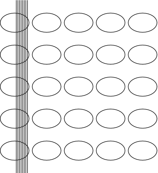


 Open access

