1. Introduction
In turbulent flow, turbulent kinetic energy is transferred from large-scale eddies to small-scale eddies, following a cascade process (Kolmogorov Reference Kolmogorov1991; Pope Reference Pope2000; Sreenivasan Reference Sreenivasan2019). To characterise this process, the velocity spectrum is often used in wavenumber space, obtained from either the temporal or spatial sequence of the flow velocity, before ensemble averaging is applied to obtain a smoother spectrum, if possible and if necessary. In physical space, space–time correlations are fundamental for characterising the dynamic coupling between spatial and temporal scales in turbulent flows, providing insights into the behaviour of turbulent fluctuations across these scales (He, Jin & Yang Reference He, Jin and Yang2017). The space–time correlation is given by
 \begin{equation} C_u(z, \tau )=\frac {\langle u(\boldsymbol{x}+{z}, t+\tau ) u(\boldsymbol{x}, t)\rangle }{u_\textit{rms}(\boldsymbol{x}) u_\textit{rms}(\boldsymbol{x}+{z})}, \end{equation}
where
 $u(\boldsymbol{x})$
is a velocity component at a spatial position
 $\boldsymbol{x}$
and
 $u_\textit{rms}(\boldsymbol{x})$
is the root-mean-square velocity (Pope Reference Pope2000; Zhou et al. Reference Zhou, Li, Lu and Liu2011; He et al. Reference He, Jin and Yang2017). In addition,
 $z$
and
 $\tau$
are the space and time separation, respectively, and
 $\langle \boldsymbol{\cdot }\rangle$
denotes the ensemble-averaging operation. The velocity temporal autocorrelation function
 $C_u(0,\tau )$
, obtained from time-series measurement at a single point, is often used in experiments (Pope Reference Pope2000; Nobach & Tropea Reference Nobach and Tropea2012). Taylor’s hypothesis can be employed to translate
 $C_u(0,\tau )$
in the time domain to
 $C_u(r,0)$
in the space domain (Taylor Reference Taylor1938). The space–time correlation has
 $C_u(z,\tau ) \approx C_u(z_T,0)$
with
 $z_T = z-U\tau$
, where
 $U$
is the convection velocity of the flow. Taylor’s hypothesis is generally valid under conditions of low turbulence intensity, negligible viscous forces and minimal mean shear (Lin Reference Lin1953; Lumley Reference Lumley1965; He et al. Reference He, Jin and Yang2017). In many turbulent flows, these flow conditions cannot be satisfied; accordingly, He & Zhang (Reference He and Zhang2006) proposed an elliptic approximation (EA) model using the second-order Taylor expansion to approximate
 $C(z,\tau )$
. In the EA model,
 $C(z,\tau ) \approx C(z_E,0)$
is established with an effective separation
 $z_E^2 = (z-U \tau )^2+V^2\tau ^2$
, where
 $U$
is the convection velocity and
 $V$
is a sweeping velocity (Zhao & He Reference Zhao and He2009; He et al. Reference He, Jin and Yang2017). When
 $U/V \gg 1$
(or
 $V\rightarrow 0$
), the EA model simplifies to Taylor’s hypothesis. When the mean flow advection vanishes (i.e.
 $U\rightarrow 0$
), the EA model reduces to the Kraichnan sweeping velocity model (Kraichnan Reference Kraichnan1964). The EA model has been validated in a variety of flows, including numerical simulations of turbulent channel flows (Guo et al. Reference Guo, Li, Zhang and He2012; Geng et al. Reference Geng, He, Wang, Xu, Lozano-Durán and Wallace2015) and simulations of planetary boundary layers (Ghate & Lele Reference Ghate and Lele2017), experiments of turbulent Rayleigh–Bénard convection (RBC) (Zhou et al. Reference Zhou, Li, Lu and Liu2011) and experiments of turbulent boundary layers (Wang, Guan & Jiang Reference Wang, Guan and Jiang2014).
When taking into consideration the passive scalar in turbulent flows, the space–time correlation of the scalar concentration,
 \begin{equation} C_\phi (z, \tau )=\frac {\langle \phi (\boldsymbol{x}+{z}, t+\tau ) \phi (\boldsymbol{x}, t)\rangle }{\phi _{{rms}}(\boldsymbol{x}) \phi _\textit{rms}(\boldsymbol{x}+{z})}, \end{equation}
is expected to display characteristics similar to those of the corresponding velocity field, given by the passive nature. Here
 $\phi$
is scalar concentration and
 $\phi _\textit{rms}$
denotes the root mean square of
 $\phi$
. He, He & Tong (Reference He, He and Tong2010) and He & Tong (Reference He and Tong2011) applied the EA model to the passive scalar (i.e. temperature) in RBC, which has a Schmidt number
 $Sc = 4.3$
(in this study, we do not distinguish between the Schmidt number (the ratio of kinematic viscosity to mass diffusivity) and the Prandtl number (the ratio of kinematic viscosity to thermal diffusivity)), to obtain the convection and the sweeping velocities. They show that using the EA model, the measured
 $C_\phi (z,\tau )$
can be converted to
 $C_\phi (z_E,0)$
where the data from different space separations collapse. The scalar spectrum
 $E_\phi (k)$
obtained from
 $C_\phi (z_E,0)$
shows distinct ranges in wavenumber space
 $k\lambda _\phi$
, where
 $k$
and
 $\lambda _\phi$
are the wavenumber and the Taylor microscale, respectively. Importantly, they show that one can use
 $ft_\phi =k\lambda _\phi$
to obtain a reliable spectrum
 $E_\phi (k)$
from single-point time-series measurements, where
 $f$
and
 $t_\phi$
are the frequency and the Taylor microtime, respectively. In later studies of RBC (where
 $Sc\approx 0.8$
), He et al. (Reference He, Funfschilling, Nobach, Bodenschatz and Ahlers2012, 2014, 2015) used the EA model to investigate RBC flow characteristics. Hogg & Ahlers (Reference Hogg and Ahlers2013) applied the EA model to the space–time correlations of shadowgraph images recorded in RBC for determining the Reynolds number parameter in the Grossmann–Lohse model.
In studies of the space–time correlation of the scalar concentration so far, the Schmidt number is around unity (i.e.
 $Sc\approx 0.8$
in air flow and
 $5$
in liquid flow). Correlation
 $C_\phi (z,\tau )$
displays similar characteristics to
 $C_u(z,\tau )$
, which is consistent with other quantities between the passive scalar and the velocity fields (e.g. Kim & Moin Reference Kim and Moin1989; Abe & Antonia Reference Abe and Antonia2009; Antonia, Abe & Kawamura Reference Antonia, Abe and Kawamura2009). In many other flows, such as water–ethanol mixing, the Schmidt number is typically of the order of
 $10^3$
(Sreenivasan Reference Sreenivasan2019). Under these high-Schmidt-number conditions, the analogy between velocity and scalar fluctuations weakens considerably, complicating predictions of flow properties and presenting challenges for accurate flow modelling and analysis (Pirozzoli Reference Pirozzoli2023). Furthermore, the spectrum of scalar fluctuations exhibits distinct characteristics depending on
 $Sc$
(as shown in figure 2 in Sreenivasan (Reference Sreenivasan2019)). For
 $Sc \sim \mathcal{O} (1 )$
, in the inertial-convective range, the spectrum is expected to scale as approximately
 $k^{-5/3}$
in homogeneous isotropic turbulence, where
 $k$
is the wavenumber. When
 $Sc\gg \mathcal{O} (1 )$
, an additional viscous-convective range emerges at smaller scales than the Kolmogorov scales with a
 $k^{-1}$
scaling in the spectrum (Batchelor Reference Batchelor1959; Kraichnan Reference Kraichnan1968), where viscosity prevails while scalar diffusion remains negligible. This range, characterised by fine-scale scalar structures, presents significant challenges for both numerical simulations and experimental measurements due to the small length scales involved (Yeung, Xu & Sreenivasan Reference Yeung, Xu and Sreenivasan2002; Gotoh & Yeung Reference Gotoh and Yeung2012). Consequently, the scaling properties of this viscous-convective range have not been well understood (Dimotakis Reference Dimotakis2005; Sreenivasan Reference Sreenivasan2019). Similarly, the characteristics of the space–time correlations (the inverse Fourier transform of the space–time energy spectra; Pope Reference Pope2000) for high-Schmidt-number passive scalar flow have been much less explored. In this study, the space–time correlations for passive scalar flows (
 $Sc\approx 2000$
) are examined in a turbulent pipe flow. In addition, the space–time correlations for the velocity field in the same turbulent pipe flow are also examined. Correspondingly, comparisons between
 $C_\phi (z,\tau )$
and
 $C_u(z,\tau )$
can be carried out, which have not yet been performed to the best of our knowledge.
The rest of this paper is organised as follows. Section 2 provides detailed descriptions of the experimental set-ups and measurement configuration, as well as the EA model. In § 3, the space–time correlations of the velocity field and scalar field are investigated, and comparisons between the two fields and discussions are presented. Finally, conclusions are drawn in § 4.
2. Methodology
2.1. Experimental configuration
The experiments are carried out in a pipe set-up, as sketched in figure 1. A constant head tank is connected to the pipe through a nozzle. The pipe is composed of several acrylic pipe segments connected with custom-made connectors. The inner pipe diameter is
 $D = 40$
mm and the pipe is 4 m (
 $=100D$
) long. A flow meter and a valve are installed at the outlet of the pipe. Purified water is the working fluid. The fluid is driven by gravity; meanwhile, the valve is adjusted to control the flow rate monitored by the flow meter. The Reynolds number is
 $Re=U_0D/\nu$
, where
 $U_0$
is the mean velocity and
 $\nu$
is the kinematic viscosity of the fluid. The Reynolds numbers in this study are
 $ Re=10\,000$
,
 $15\,000$
and
 $20\,000$
. A dilute concentration (100 μg l−1) of fluorescent dye (Rhodamine 6G; Schmidt number is about
 $2000$
) is used as the passive scalar. To release the fluorescent dye into the turbulent pipe flow, an L-shaped injector is installed through a small hole in the pipe wall, as schematically illustrated in figure 1. The horizontal part of the injector is at the pipe centre and aligned with the pipe axis. The inner diameter of the injector is
 $d=2$
mm and the outer diameter of the injector is
 $2.4$
mm. A gear pump (LEADFLUID CT3001F) is used to discharge the fluorescent dye into the pipe. The fluorescent dye is continuously discharged and the discharge flow rate is precisely controlled to match the mean velocity, in order to reduce the perturbation of the discharge flow to the turbulence. The Cartesian coordinate system is set such that the origin (
 $O$
) is at the intersection point of the pipe axis and the left border of the field of view,
 $Z$
is along the pipe axis and
 $X$
is along the pipe radius.
Sketch of the experimental set-up. The Cartesian coordinates are indicated by red arrows.

The planar laser-induced fluorescence (PLIF) technique is implemented to measure the passive scalar mixing in the
 $X{-}Z$
plane. The measurement field of view is about
 $1.2D\times 1.2D$
, about
 $220d$
from the injector exit, which is far away from
 $2d$
as demonstrated by Villermaux & Innocenti (Reference Villermaux and Innocenti1999). Besides, the disturbances of the injector and discharge flow to the base turbulent flow are examined through the probability density function distributions of concentration fluctuations and are very small and ignorable (see Li, Xu & He Reference Li, Xu and He2025). The laser sheet is formed by a group of optical lenses. The average thickness of the laser sheet for the field of view is about
 $200$
μm. A high-repetition-rate pulse laser is used for illumination. To correct the laser intensity variation in the PLIF measurements, a photodetector is used to monitor the intensity of laser pulses simultaneously with the PLIF measurements. The PLIF images are recorded at a sampling rate (
 $f$
) of
 $1000$
Hz and the photodetector measurements are at a sampling rate of
 $40\,000$
Hz. The signal of the photodetector averaged per pulse is used for correction. Approximately 10 000 PLIF images are captured per Reynolds number, covering a duration of about
 $60D/U_0$
. The calibration of the PLIF measurements follows the procedure detailed in Xu & Chen (Reference Xu and Chen2012). The configurations of the measurement hardware in the mixing measurements are kept unchanged from the calibration. The maximum relative uncertainty of the concentration measurements is about 1 %.
Two-dimensional particle image velocimetry (PIV) is used to measure the flow velocity in the
 $X{-}Z$
plane, separately from the PLIF measurements. Hollow glass spheres with a median diameter of about 11 μm are used as the tracers. The same illumination and camera configurations as in the PLIF measurements are used for the PIV measurements. The sampling rate (
 $f$
) is tuned for each
 $ Re$
to maintain maximum particle displacements of about 8 pixels, adhering to the one-quarter rule for the interrogation window size at the last step of the multi-step algorithm (Raffel et al. Reference Raffel, Willert, Scarano, Kähler, Wereley and Kompenhans2018), where the interrogation window is
 $64\times 64$
px
 $^2$
at the initial step and
 $32\times 32$
px
 $^2$
at the last step with a
 $50\,\%$
window overlap. A subpixel Gaussian interpolation is used (Raffel et al. Reference Raffel, Willert, Scarano, Kähler, Wereley and Kompenhans2018) and the uncertainty is around 0.1 px or smaller (from Lavision Davis software; see Wieneke (Reference Wieneke2015)). For each Reynolds number, approximately 10 000 instantaneous velocity fields are obtained.
2.2. Elliptic approximation model
The EA model was proposed to account for the space–time correlation of flow velocity in turbulent flows (He & Zhang Reference He and Zhang2006; Zhao & He Reference Zhao and He2009; He et al. Reference He, Jin and Yang2017). For completeness of this paper, the key derivation is summarised here. In the EA model, the correlation function
 $C_u(z,\tau )$
is expanded to second order in a Taylor series as follows:
 \begin{equation} \begin{aligned} C_u(z, \tau )\,=\, & C_u(0,0)+\frac {\partial C_u(0,0)}{\partial z} z+\frac {\partial C_u(0,0)}{\partial \tau } \tau \\ & +\frac {\partial ^2 C_u(0,0)}{\partial z \partial \tau } z \tau +\frac {1}{2}\left [\frac {\partial ^2 C_u(0,0)}{\partial z^2} z^2+\frac {\partial ^2 C_u(0,0)}{\partial \tau ^2} \tau ^2\right ]+\cdots . \end{aligned} \end{equation}
Here,
 $z$
and
 $\tau$
are the separation length and time, respectively. For spatially homogeneous and statistically stationary turbulence, the first-order derivatives vanish (He & Zhang Reference He and Zhang2006). Thus, (2.1) simplifies to
 \begin{equation} C_u(z, \tau )=C_u(0,0)+\frac {1}{2} \frac {\partial ^2 C_u(0,0)}{\partial z^2} z_E^2, \end{equation}
where
 \begin{equation} z_E^2=(z-U \tau )^2+V^2 \tau ^2. \end{equation}
The terms
 $U$
and
 $V$
are given by
 \begin{equation} U=-\frac {\partial ^2 C_u(0,0)}{\partial z \partial \tau }\left [\frac {\partial ^2 C_u(0,0)}{\partial z^2}\right ]^{-1} \end{equation}
and
 \begin{equation} V^2=\frac {\partial ^2 C_u(0,0)}{\partial \tau ^2}\left [\frac {\partial ^2 C_u(0,0)}{\partial z^2}\right ]^{-1}-U^2, \end{equation}
where
 $U$
is the advection velocity and
 $V$
is the sweeping velocity from the velocity fluctuation. From the isocorrelation curves of the correlation
 $C_u$
, it can be found that
 \begin{equation} C_u(z,0) = C_u(0,\tau ), \end{equation}
where
 $z = \sqrt {U^2+V^2}\tau$
. For small values of
 $z$
and
 $\tau$
,
 $C_u(z,0)$
and
 $C_u(0,\tau )$
can be expanded as
 \begin{equation} \begin{aligned} & C_u(z, 0)=1-\left (\frac {z}{\lambda _z}\right )^2+\cdots , \\ & C_u(0, \tau )=1-\left (\frac {\tau }{\lambda _\tau }\right )^2+\cdots , \end{aligned} \end{equation}
where
 $\lambda _z$
is the Taylor microscale in space and
 $\lambda _\tau$
is the Taylor microscale in time.
The characteristic velocities
 $U$
and
 $V$
in the EA model can be obtained from the conditions
 $\partial z_E/\partial z|_\tau = 0$
and
 $\partial z_E/\partial \tau |_r = 0$
(Zhou et al. Reference Zhou, Li, Lu and Liu2011; Hogg & Ahlers Reference Hogg and Ahlers2013; He & Tong Reference He and Tong2014), yielding that
 \begin{equation} z_p = U\tau \end{equation}
and
 \begin{equation} \tau _p = \frac {U}{U^2+V^2} z, \end{equation}
where
 $C_u(z,\tau )$
is maximised at
 $z_p$
for a given
 $\tau$
, and similarly maximised at
 $\tau _p$
for a given
 $z$
(He et al. Reference He, He and Tong2010). For a given time separation
 $\tau$
,
 $z_p$
can be determined by fitting a Gaussian curve to the correlation function
 $C_u(z,\tau )$
, i.e.
 \begin{equation} C_u\left (z, \tau \right )=C_0 \exp \big[(z-z_p)^2 /\big(2 C_1^2\big)\big ]+C_2, \end{equation}
where
 $C_0$
,
 $C_1$
and
 $C_2$
are free parameters. By repeating the curve-fitting process across different values of
 $\tau$
, the corresponding
 $z_p$
values are obtained. Then,
 $U$
is obtained by performing a linear fit of
 $z_p$
versus
 $\tau$
in accordance with (2.8). Similarly, for a given spatial separation
 $z$
, we fit
 $C_u(z,\tau )$
as a function of
 $\tau$
using
 \begin{equation} C_u (z, \tau)=C_3 \exp \big [ (\tau -\tau _p)^2 /\big(2 C_4^2\big)\big]+C_5 \end{equation}
to obtain
 $\tau _p$
, where
 $C_3$
,
 $C_4$
and
 $C_5$
are fitting parameters. By repeating the curve-fitting process over the available spatial separation
 $z$
, the corresponding
 $\tau _p$
can be obtained. A linear fit of
 $\tau _p$
versus
 $z$
then gives
 $U/(U^2 + V^2)$
, from which the sweeping velocity
 $V$
can be computed.
3. Results and discussion
3.1. Elliptic approximation for flow velocity
The space–time correlation
 $C_u(z,\tau )$
is analysed using the streamwise velocity component and the length separation along the pipe axis, especially at radial positions
 $r/D=0$
(pipe centre), 0.2, 0.3 and 0.4. At the pipe centre, where the mean shear is approximately zero, the fluctuation velocity is smaller compared with the mean velocity, and Taylor’s hypothesis is usually employed in studies (e.g. van Doorne & Westerweel Reference van Doorne and Westerweel2007; Ganapathisubramani, Lakshminarasimhan & Clemens Reference Ganapathisubramani, Lakshminarasimhan and Clemens2007; Lopez, Choueiri & Hof Reference Lopez, Choueiri and Hof2019). Closer to the wall, the velocity fluctuations increase and shear effects become more significant, Taylor’s hypothesis leaves the ideal circumstance for application. Figure 2(a–d) presents the contours of
 $C_u(z,\tau )$
at
 $r/D=0$
to
 $0.4$
for
 $ Re= 10\,000$
, illustrating the space–time correlation with space separation
 $z$
and time separation
 $\tau$
, and the corresponding isocorrelation curves are plotted in figure 2(e–h). The
 $C_u(z,\tau )$
exhibits a decay along both the separations
 $z$
and
 $\tau$
. The isocorrelation contours exhibit self-similarity and share the same preferred orientation and aspect ratio. It is noted that
 $C_u(z,\tau )$
decays relatively slowly along the preferential direction (i.e. the elliptical major axis) but declines more rapidly along the perpendicular direction (i.e. the elliptical minor axis) at
 $r/D = 0$
. Here the isocorrelation contours of
 $C_u(z,\tau )\approx 0.5$
appear as straight lines, as shown in figure 2(a,e). The decay of the correlation becomes faster at
 $r/D=0.3$
and
 $0.4$
along the preferential direction. For instance, the isocorrelation contours of
 $C_u(z,\tau )\approx 0.5$
are shortened along the preferential direction and expanded along the perpendicular direction, more like an ellipse, in agreement with the EA description.
(a–d) Space–time correlations
 $C_u$
as a function of
 $z$
and
 $\tau$
at
 $r/D = 0$
(a), 0.2 (b), 0.3 (c) and 0.4 (d) for Re = 10 000. (e–h) The corresponding isocorrelation contours of
 $C_u(z,\tau )$
with the colour-coded correlation amplitude varying from 0.2 to 0.8 with an increment of 0.1.

The characteristic velocities
 $U$
and
 $V$
in (2.3) are determined following the procedure introduced in § 2.2. Our results for the measured
 $z_p$
as a function of time separation
 $\tau$
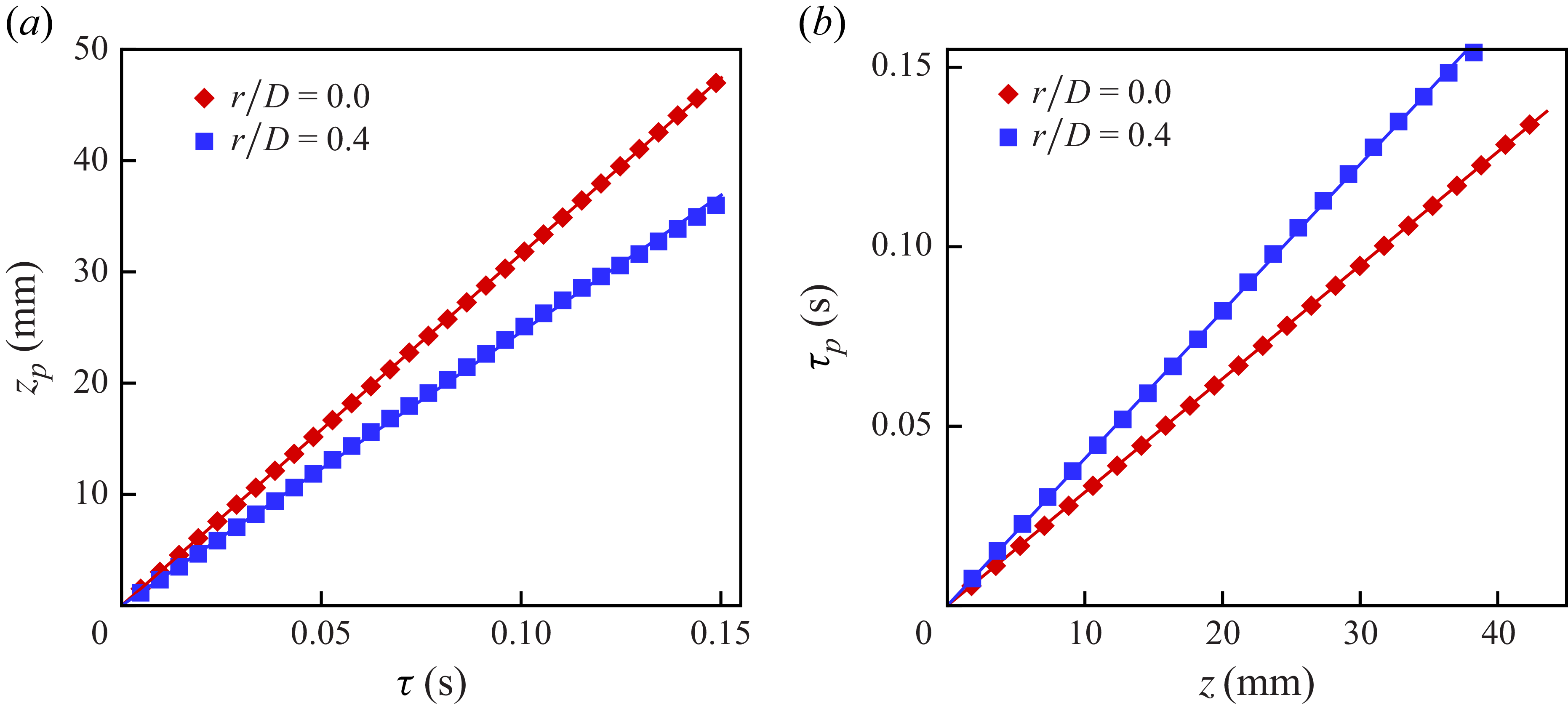
(i.e. (2.8)) are shown in figure 3(a). As expected,
 $z_p$
increases with the increase of
 $\tau$
, which indicates that a longer time lag is required to transport velocity fluctuations across a larger separation. Notably, this relationship appears to be linear,
 $z_p = U\tau$
, where
 $U \approx 315.7$
mm s−1 at
 $r/D = 0$
and
 $U \approx 245.9$
mm s−1 at
 $r/D = 0.4$
. Similarly, figure 3(b) displays that the measured
 $\tau _p$
varies with the separation
 $r$
. Similar to the behaviour of
 $z_p$
,
 $\tau _p$
increases linearly with the increase of
 $z$
, as suggested by (2.9). A linear fitting to the data yields that
 $U/(U^2+V^2)$
 $\approx$
 $3.16\times 10^{-3}$
s mm−1 at
 $r/D = 0.0$
and
 $U/(U^2+V^2)$
 $\approx$
 $3.98\times 10^{-3}$
s mm−1 at
 $r/D = 0.4$
. Correspondingly, the sweeping velocity is
 $V\approx 15.44$
mm s−1 and
 $V\approx 35.66$
mm s−1 at
 $r/D = 0$
and
 $r/D = 0.4$
, respectively.
(a) The measured peak position
 $z_p$
as a function of
 $\tau$
for the velocity field at Re = 10 000. The solid line shows the corresponding fitted linear function,
 $z_p = U \tau$
, with
 $U(r/D = 0.0) \approx 316.08$
mm s−1 and
 $U(r/D = 0.4) \approx 245.92$
mm s−1. (b) The measured peak position
 $\tau _p$
as a function of
 $z$
. The solid line shows the corresponding fitted linear function,
 $\tau _p = [U/(U^2 + V^2)]z$
with
 $U/(U^2+V^2)$
 $\approx$
 $3.16 \times 10^{-3}$
s mm−1 at
 $r/D = 0$
and
 $U/(U^2+V^2)$
 $\approx$
 $3.98\times 10^{-3}$
s mm−1 at
 $r/D = 0.4$
.

Figure 4 shows that the profiles of the convection velocity
 $U$
and sweeping velocity
 $V$
along the pipe radius for different Reynolds numbers. As
 $r/D$
increases, the convection velocity decreases while the sweeping velocity increases. The trend of the former aligns with the results from Kim & Hussain (Reference Kim and Hussain1993) for channel flow. In the centre region of the pipe (
 $r/D \lesssim 0.2$
), the convection velocity decreases slowly with the increase of
 $r/D$
and
 $U/V \gg 1$
, which meets the ideal application condition of Taylor’s hypothesis, corresponding to the straight lines of the isocorrelation contour (in figure 2). For
 $r/D \gtrsim 0.3$
, as
 $r/D$
increases, the convection velocity decreases rapidly and the sweeping velocity increases, leading to
 $U$
and
 $V$
being of comparable magnitude. In this region,
 $U/V\gg 1$
does not hold, suggesting that Taylor’s hypothesis is not valid here, and both the convection and sweeping effects contribute to the turbulence transport dynamics.
The normalised convection velocity
 $U$
(a) and sweeping velocity
 $V$
(b) of the velocity field along the pipe radius,
 $U_c$
being the ensemble average streamwise velocity at the pipe centre. The cyan dashed symbol line is the convection velocity from Kim & Hussain (Reference Kim and Hussain1993) for channel flow. Error bars in both panels indicate 95 % confidence bounds for the fitted
 $ U$
and
 $ V$
. Insets display the convection and sweeping velocities in wall units, where
 $ y = (D/2 - r)$
is the wall-normal distance, and the superscript
 $+$
denotes non-dimensionalisation using kinematic viscosity
 $ \nu$
and friction velocity
 $ u_\tau$
. The insets confirm that measurements are taken far from the wall. The friction velocity is determined from the relationship between
 $ u_\tau$
and
 $ Re$
reported in Draad, Kuiken & Nieuwstadt (Reference Draad, Kuiken and Nieuwstadt1998). Symbols are omitted for clarity.

Using the obtained values of
 $U$
and
 $V$
, the relation between
 $C_u(z,\tau )$
and
 $C_u(z_E,0)$
can be explored. Figures 5(a) and 5(d) show the change of
 $C_u(z,\tau )$
as a function of the space separation
 $z$
for several
 $\tau$
at
 $r/D = 0$
and
 $r/D = 0.4$
, respectively. In these two plots, each
 $C_u(z,\tau )$
curve exhibits a single peak at position
 $z_p$
. The
 $z_p$
shifts to larger values as
 $\tau$
increases, while the correlation amplitude of
 $C_u(z_p)$
gradually decreases. This trend shows that velocity fluctuations decorrelate as the space separation increases. Figure 5(b,e) shows the measured
 $C_u$
against the Taylor’s hypothesis separation
 $z_T$
in semi-logarithmic plots to highlight the small separation. Figure 5(c, f) shows the measured
 $C_u$
against the EA separation
 $z_E$
from (2.3) using the obtained values of
 $U$
and
 $V$
. The results show an approximate collapse of the correlation curves, especially for small-time separation, confirming that the space–time correlations
 $C_u(z,\tau )$
can be described by
 $C_u(z_E,0)$
with
 $z_E$
given in (2.3), comparing with Taylor’s hypothesis.
The space–time correlations
 $C_u$
obtained at
 $r/D=0$
(a–c, sharing the same legend) and
 $r/D = 0.4$
(d–f, sharing the same legend) for
 $ Re=10\,000$
. Correlations (b,e)
 $C_u$
versus the separation
 $z_T = z-U \tau$
and (c, f)
 $C_u$
versus the separation
 $z_E = \sqrt {(z-U \tau )^2+(V \tau )^2}$
with
 $U$
and
 $V$
obtained from figure 3.

Direct comparison between the two sample spatial velocity fluctuation profiles reconstructed using Taylor’s hypothesis (
 $z_T = -U\tau$
) and the EA model (
 $z_E = -\sqrt {U^2+V^2}\tau$
) from the same time series at
 $r/D = 0$
(a) and
 $r/D = 0.4$
(b) for Re = 10 000. The velocity is normalised by the bulk mean velocity
 $U_0$
. The velocity spectrum
 $E_u$
as a function of the wavenumber
 $k\eta _{\scriptscriptstyle K}$
, where
 $\eta _{\scriptscriptstyle K}$
is the Kolmogorov length scale, for
 $r/D = 0$
(c) and
 $r/D = 0.4$
(d), where the time-series data at
 $(z/D,r/D)=(0,0)$
and
 $(z/D,r/D)=(0,0.4)$
are converted to the space series using Taylor’s hypothesis and the EA model before obtaining the spectra.

To clarify the difference between Taylor’s hypothesis and the EA model, the space series of velocity reconstructed using the time series at a point is shown in figures 6(a) and 6(b) for
 $r/D=0$
and
 $r/D=0.4$
, respectively. At the pipe centre (shown in figure 6
a), the velocity series from the two methods are very similar, but a distinct difference can be observed at
 $r/D = 0.4$
(see figure 6
b), where the data series from the EA model has a clear shift to larger
 $z_E$
. In figures 6(c) and 6(d), the velocity spectrum
 $E_u$
using one-dimensional space data is shown for
 $r/D=0$
and
 $r/D=0.4$
, respectively. In addition, the velocity spectra obtained by the time series after being converted to space using the EA model and Taylor’s hypothesis are also shown, and they approximately agree with the spectrum obtained using the space data, although fluctuations can be clearly observed. Similar fluctuations in the spectrum can also be observed in Rosenberg et al. (Reference Rosenberg, Hultmark, Vallikivi, Bailey and Smits2013) and Vallikivi, Ganapathisubramani & Smits (Reference Vallikivi, Ganapathisubramani and Smits2015), where the spectrum is also obtained using the time series of a single-point measurement.
3.2. Space–time correlation of passive scalar
The space–time correlation
 $C_\phi$
for the passive scalar is obtained using (1.2). Correlation
 $C_\phi$
is obtained with space separation
 $z$
along the streamwise direction. Figure 7(a–d) shows the contours of
 $C_\phi (z,\tau )$
at Re = 10 000. Multiple local peaks can be observed in
 $C_\phi (z,\tau )$
. This is a result of the insufficient temporal sampling rate of the passive scalar field, compared with the measurement spatial resolution and the flow advection speed. For this Reynolds number, the spatial resolution is about 27 μm, correspondingly the current sampling rate of
 $1$
kHz is far less than the approximate
 $U_c/\eta _B \approx 53$
kHz and the rendering in contours possibly leads to the visual local peaks for large
 $C_\phi$
(see discussion in § 3.4). Regardless of these peaks, the amplitude of
 $C_\phi$
decays as
 $z$
and (or)
 $\tau$
increase(s). Figure 7(e–h) displays corresponding isocorrelation curves of
 $C_\phi$
. As
 $r/D$
increases, the isocorrelation contours decay more quickly along the preferential direction and more slowly along the perpendicular direction. The isocorrelation contours display closed elliptic-like curves, maintaining a consistent orientation and aspect ratio, sharing the same characteristics as
 $C_u(z,\tau )$
. In the turbulent RBC study of He et al. (Reference He, He and Tong2010), the fluctuations of velocity and passive scalar (i.e. temperature with
 $Sc \sim 1$
) are assumed to share similar decorrelation mechanisms, suggesting that
 $C_\phi$
may exhibit a scaling behaviour similar to that of
 $C_u$
. In the present study, although the correlation decay rates of
 $C_\phi$
differ from those of
 $C_u$
, due to the influence of high
 $Sc$
on scalar mixing dynamics, the isocorrelation contours of the scalar field retain elliptical shapes. This structural similarity leads us to assume that the EA model is applicable to the passive scalar field to estimate the convection and sweeping velocities of the scalar field.
Space–time correlations
 $C_\phi$
as a function of
 $z$
and
 $\tau$
at
 $r/D = 0$
(a,e), 0.2 (b,f), 0.3 (c,g) and 0.4 (d,h) for Re = 10 000. The isocorrelation contours (e–h) of
 $C_\phi$
with the colour-coded correlation amplitudes varying from 0.2 to 0.8 with an increment of 0.1.

Following the process outlined in § 2.2, the scalar fluctuations are analysed to derive characteristic velocities of the correlation function
 $C_\phi$
, with
 $U_\phi$
denoting the convection velocity and
 $V_\phi$
representing the sweeping velocity for the scalar field. Also, with analogy to the velocity field, the peak position of
 $C_\phi$
is fitted using a Gaussian curve in space and time separation, respectively, for a given separation, following (2.10) and (2.11). The results for the peak position
 $z_{p}$
as a function of time separation
 $\tau$
are shown in figure 8(a) and
 $\tau _{p}$
as a function of time separation
 $z_\phi$
is shown in figure 8(b). Within the separations shown, both
 $z_{p}$
and
 $\tau _{p}$
increase linearly with
 $\tau$
and
 $z$
, respectively. Linearly fitting the data in figure 8 yields
 $U_\phi \approx 318.01$
mm s−1 and
 $V_\phi \approx 8.62$
mm s−1 at the pipe centre, and
 $U_\phi \approx 268.22$
mm s−1 and
 $V_\phi \approx 85.39$
mm s−1 at
 $r/D = 0.4$
, using (2.8) and (2.9).
The profiles of convection and sweeping velocities along the pipe radius are plotted in figure 9. At
 $r/D=0$
, the convection velocity
 $U_\phi$
is approximately
 $0.97U_c$
, where
 $U_c$
denotes the ensemble-average streamwise velocity at
 $r/D=0$
. Velocity
 $U_\phi$
decreases slightly along the pipe radius until
 $r/D\approx 0.2$
. Beyond
 $r/D \approx 0.2$
, a remarkable decrease in convection velocity is observed. In contrast, the sweeping velocity
 $V_\phi$
increases along the pipe radius. At
 $r/D=0$
,
 $U_\phi /V_\phi \gg 1$
, indicating that the scalar fluctuations are primarily governed by the convection velocity, which aligns with the requirement of Taylor’s hypothesis. However, for
 $r/D\gt 0.3$
, where the flow shear effects become strong,
 $U_\phi /V_\phi \lt 5$
, showing that both convection and sweeping effects contribute comparably to scalar transport. This means that, in such regions, small-scale scalar fluctuations are distorted by large-scale shearing and small-scale interactions, instead of being ‘frozen’ as assumed under Taylor’s hypothesis. Thus, the limitations of Taylor’s hypothesis are apparent for scalar transport, and the EA model is more suitable for describing the scalar transport dynamics.
(a) The extracted peak position
 $z_{p}$
as a function of
 $\tau$
for the passive scalar field at Re = 10 000. The solid line represents the corresponding fitted linear function,
 $z_{p} = U_\phi \tau$
. (b) The measured peak position
 $\tau _{p}$
as a function of
 $z$
. The solid line shows the fitted linear function,
 $\tau _{p} = [U_\phi /(U_\phi ^2+V_\phi ^2)]z$
.

The normalised convection velocity
 $U_\phi /U_c$
(a) and sweeping velocity
 $V_\phi /U_c$
(b) of the passive scalar field along the pipe radius. Error bars in both panels indicate 95 % confidence bounds. Symbols are omitted for clarity.

Furthermore, figures 10(a) and 10(d) show the space–time correlations for several time separations
 $\tau$
at
 $r/D=0$
and
 $r/D=0.4$
, respectively. For a given time separation,
 $C_\phi (z_{p})$
decays faster at
 $r/D = 0.4$
than at
 $r/D = 0$
. In addition,
 $C_\phi (z)$
is broader at
 $r/D=0.4$
than at
 $r/D=0$
. The measured
 $C_\phi (z)$
is shown in figure 10(b,e) as function of
 $z_T=U\tau$
using Taylor’s hypothesis for the corresponding
 $r/D$
, where
 $C_\phi$
at
 $r/D=0.4$
shows a distinct difference for the time separations at small
 $z_T$
. With respect to
 $U_\phi$
and
 $V_\phi$
in figure 8, the measured
 $C_\phi (z)$
are also converted to be a function of
 $z_E$
(2.3) for the corresponding
 $r/D$
, as shown in figure 10(c, f). Here, by analogy to the velocity field,
 $z_E = \sqrt {(z-U_\phi \tau )^2+(V_\phi \tau )^2}$
with the corresponding
 $U_\phi$
and
 $V_\phi$
. At the pipe centre,
 $C_\phi$
exhibits a collapse onto a master curve and its peak amplitude decreases as
 $z_E$
increases. In addition,
 $C_\phi \approx 0$
at
 $z_E\approx 1.5$
, representing the decorrelation length. At
 $r/D = 0.4$
,
 $C_\phi (z_E)$
from different
 $\tau$
shows much better collapse than
 $C_\phi (z_T)$
. The peak amplitude of
 $C_\phi$
decreases but the correlation width broadens with the increase of
 $z_E$
, giving
 $z_E\approx 10$
for
 $C_\phi \approx 0$
. The broadening of
 $C_\phi$
demonstrates that at larger
 $r/D$
the decorrelation is established with larger separation distance. The approximately collapsed
 $C_\phi (z_E, 0)$
suggests that the EA model for the scalar concentration field is valid, in agreement with the expectation in He et al. (Reference He, He and Tong2010, Reference He, van Gils, Bodenschatz and Ahlers2015).
The space–time correlations
 $C_\phi$
versus the space separation
 $z$
at
 $r/D=0$
(a–c) and
 $r/D = 0.4$
(d–f) for
 $ Re=10\,000$
. Correlations (b,e)
 $C_\phi$
versus the separation
 $z_T = z-U_\phi \tau$
and (c, f)
 $C_\phi$
versus the separation
 $z_E = \sqrt {(z-U_\phi \tau )^2+(V_\phi \tau )^2}$
with
 $U_\phi$
and
 $V_\phi$
obtained from figure 8.

Time-series scalar fluctuation profiles reconstructed using Taylor’s hypothesis
 $(z_T = -U_\phi \tau )$
and the EA model
 $(z_E = -\sqrt {U_\phi ^2+V_\phi ^2}\tau )$
at
 $r/D = 0$
(a) and
 $r/D = 0.4$
(b) for Re = 10 000. The scalar spectrum
 $E_\phi$
from the one-dimensional spatial data and the spatial data converted from the time series using the EA model at
 $r/D=0$
(c) and
 $r/D=0.4$
(d), where the time-series data at
 $(z/D,r/D)=(0,0)$
and
 $(z/D,r/D)=(0,0.4)$
are converted to the space series using Taylor’s hypothesis and the EA model before obtaining the spectra. The grey dash-dot lines indicate the scaling
 $k^{-4/3}$
(e.g. Sreenivasan Reference Sreenivasan1991; Lohse Reference Lohse1994) and
 $k^{-1}$
(e.g. Batchelor Reference Batchelor1959; Kraichnan Reference Kraichnan1968) from small to large wavenumbers.

The time-series data of the scalar fluctuation at
 $r/D = 0$
and
 $0.4$
are converted to the corresponding space series using Taylor’s hypothesis and the EA model, and they are shown in figures 11(a) and 11(b), respectively. The curves from the two methods are nearly collapsed at
 $r/D=0$
, and are visually similar at
 $r/D=0.4$
but with a noticeable shift. For instance, in figure 11(b), a peak of the scalar fluctuation is observed around
 $z_T \approx 180$
, but it is clear that this scalar fluctuation has a different spatial coordinate under the EA model. The discrepancy of the converted fluctuation in space between Taylor’s hypothesis and the EA model increases with the increase of
 $z_E$
.
The time-series data from a spatial point at
 $r/D=0$
and
 $r/D=0.4$
are converted to the corresponding space data using the EA model. The spectra of the scalar fluctuations
 $E_\phi$
are obtained using the one-dimensional space data and the converted data from the time series, as shown in figures 11(c) and 11(d) for
 $r/D = 0$
and
 $r/D = 0.4$
, respectively. At
 $r/D = 0$
, where the camera pixel resolution and laser sheet thickness provide a spatial resolution closest to the Batchelor length scale in the present measurement,
 $E_\phi$
shows a narrow band of approximate
 $k^{-4/3}$
scaling in the inertial-convection range (as also noted in scalar mixing in other shear flows; e.g. Sreenivasan Reference Sreenivasan1991; Lohse Reference Lohse1994) and the incipient
 $k^{-1}$
scaling in the viscous-convection range (e.g. Batchelor Reference Batchelor1959; Kraichnan Reference Kraichnan1968; Gotoh & Yeung Reference Gotoh and Yeung2012; Sreenivasan Reference Sreenivasan2019). In contrast, at
 $r/D = 0.4$
, the
 $k^{-1}$
scaling is not observed in the spectrum, possibly due to the non-trivial flow shear and/or insufficient measurement resolution to resolve the Batchelor scale.
3.3. Comparison between velocity and scalar fields
In §§ 3.1 and 3.2, the space–time correlations for the velocity and the scalar fields have been examined and both correlations display elliptical characteristics. However, distinctions between the two correlations can be observed in that
 $C_\phi$
is much narrower than
 $C_u$
, indicating that the scalar fluctuations decorrelate faster in either space or time than the corresponding velocity fluctuations. From the correlations, the Taylor microscale can be estimated by using the equation
 $C_u \simeq 1-(z_E/\lambda _u)^2$
in the velocity field (Pope Reference Pope2000; Zhou et al. Reference Zhou, Li, Lu and Liu2011) and
 $C_\phi \simeq 1-(z_E/\lambda _\phi )^2$
(He et al. Reference He, He and Tong2010, Reference He, van Gils, Bodenschatz and Ahlers2014) in the scalar field for very small
 $z_E$
. In this study, three points near
 $z_E = 0$
were used for the estimation of the Taylor microscale. The curve fitting for the correlations presented in figures 5(c) and 10(c) gives
 $\lambda _u \approx 4.21$
mm for the velocity field and
 $\lambda _\phi \approx 0.14$
mm for the scalar field, respectively, showing that
 $\lambda _\phi /\lambda _u \approx 1/30$
. This is in agreement with
 $\lambda _\phi /\lambda _u \ll 1$
in isotropic turbulence with
 $Sc\gg 1$
(George Reference George1992). In RBC, He et al. (Reference He, He and Tong2010) reported
 $\lambda _\phi \approx 8.5$
mm for
 $Sc \approx 4.3$
and Rayleigh number
 $Ra\approx 1.4 \times 10^{10}$
. Similarly, in the RBC of Zhou et al. (Reference Zhou, Li, Lu and Liu2011),
 $\lambda _u\approx 18.2$
mm (estimated using their correlation data in figure 5
c) for
 $Sc \approx 5.5$
and
 $Ra\approx 9.5 \times 10^{10}$
. If the effect of the Rayleigh number is assumed to be small on the Taylor microscale, the Taylor microscales from these two RBC studies can be put together for comparison, affording
 $\lambda _\phi /\lambda _u\lt 1$
for
 $Sc \approx 5$
.
A direct comparison of the convection velocity and sweeping velocity between the velocity field (shown in figure 4) and the passive scalar field (presented in figure 9) is shown in figure 12. For the convection velocity, the ratio
 $U_\phi /U$
increases gradually with
 $r/D$
when
 $r/D\lt 0.1$
and rapidly for
 $0.1\lt r/D\lt 0.2$
. Then
 $U_\phi /U$
increases gradually again for
 $0.2\lt r/D\lt 0.35$
and more rapidly for
 $r/D \gt 0.35$
. In contrast, for the sweeping velocity,
 $V_\phi /V$
increases rapidly with
 $r/D$
for
 $r/D \lt 0.1$
, then
 $V_\phi /V$
is nearly constant for
 $0.1\lt r/D\lt 0.3$
, followed by another rapid increase for
 $r/D \gt 0.3$
. Importantly, the increase of
 $U_\phi /U$
and
 $V_\phi /V$
continues as
 $r/D$
increases. A few rational questions arise but cannot be answered in this study, such as, Is there a peak for
 $U_\phi /U$
and
 $V_\phi /V$
?, What is
 $r/D$
for the peak?, What is the physical mechanism behind it? and What is the effect of Schmidt number on this ratio?
(a) The convection velocity ratio between the velocity field and the passive scalar field. (b) The sweeping velocity ratio between the velocity field and the passive scalar field. Error bars are calculated using error propagation. Symbols are omitted for clarity.

Wavenumber-dependent convection velocities. Dashed lines with open symbols represent the velocity field (
 $ U_k^u$
) and solid lines with filled symbols represent the scalar field (
 $ U_k^\phi$
). The grey region is selected for comparison, with results shown in the inset. Symbols in the inset match the radial positions in the legend. Symbols are omitted for clarity.

To further understand the differences between the convection velocity in the scalar and velocity fields, the wavenumber-dependent convection velocity
 $ U_k(k)$
is calculated (Del Álamo & Jiménez Reference Del Á lamo and Jiménez2009; Wu & He Reference Wu and He2021a
,
Reference Wu and Heb
):
 \begin{equation} U_k(k) = \frac {f_c(k)}{k}, \quad \text{where} \quad f_c(k) = \frac {\int f E(k,f) {\textrm{d}}f}{\int E(k,f) {\textrm{d}}f}. \end{equation}
Here
 $f_c(k)$
is the mean frequency of space–time energy spectra
 $E(k,f)$
at a given wavenumber
 $k$
. Equation (3.1) provides a general formulation. In this study, the wavenumber-dependent convection velocities for
 $ U_k^\phi$
(scalar field) and
 $ U_k^u$
(velocity field) are calculated using their respective space–time energy spectra, namely
 $ E_\phi (k,f)$
for the scalar field and
 $ E_u(k,f)$
for the velocity field, according to (3.1). Besides, the convection velocity (
 $ U$
in figure 4 and
 $ U_\phi$
in figure 9) can be understood as the weighted average of the wavenumber-dependent convection velocities:
 \begin{equation} U = \frac {\int U_k^u k^2 E_u(k) {\textrm{d}} k}{\int k^2 E_u(k) {\textrm{d}} k} \quad \text{and} \quad U_\phi = \frac {\int U_k^\phi k^2 E_\phi (k) {\textrm{d}} k}{\int k^2 E_\phi (k) {\textrm{d}} k}, \end{equation}
where the space spectra
 $E_u(k) = \int E_u(k,f){\textrm{d}} f$
and
 $E_\phi (k) = \int E_\phi (k,f){\textrm{d}} f$
. The results for
 $ U_k^\phi$
(scalar field) and
 $ U_k^u$
(velocity field) are presented in figure 13. For the velocity field,
 $ U_k^u$
slightly increases with wavenumber and then decreases slightly for
 $ r/D \leqslant 0.3$
, indicating that the fluctuations at medium wavelengths propagate slightly faster. Notably, at
 $ r/D = 0.3$
, the peak velocity occurs at small wavenumbers (see the green dashed line with open symbols in figure 13). For
 $ r/D = 0.4$
,
 $ U_k^u$
decreases as wavenumber increases, meaning that the fluctuations at longer wavelengths propagate relatively faster. These trends align with observations in channel flows (e.g. Del Álamo & Jiménez Reference Del Á lamo and Jiménez2009; Wu & He Reference Wu and He2021b
). The rapid increase in the convection velocity ratio near
 $ r/D = 0.3$
may be due to near-wall effects, where the wall’s influence alters the flow dynamics. For the scalar field,
 $ U_k^\phi$
shows a pattern of slight increase followed by a decrease for all
 $ r/D$
. Additionally, at the same
 $ r/D$
,
 $ U_k^\phi$
is consistently larger than
 $ U_k^u$
, as highlighted in the inset of figure 13. This suggests that the passive scalar field is more readily propagated by the turbulent field. Consequently, the weighted average of the wavenumber-dependent convection velocities for the scalar field (
 $ U_\phi$
) exceeds that of the velocity field (
 $ U$
). Regarding the sweeping velocity, it can be understood that
 $ V$
is primarily influenced by the root-mean-square fluctuation of velocity or scalar (Hogg & Ahlers Reference Hogg and Ahlers2013). For high-Schmidt-number passive scalar fields, scalar fluctuations are more pronounced compared with those in scalar fields with
 $ Sc = 1$
(Antonia & Orlandi Reference Antonia and Orlandi2003; Buaria et al. Reference Buaria, Clay, Sreenivasan and Yeung2021) (the sweeping velocity of the latter is assumed to be similar to that of the velocity field). Thus, the enhanced fluctuations in the scalar field may lead to an increase in the scalar sweeping velocity. Previous studies have shown that convection velocities in the velocity field vary with specific flow variables or structures (Kim & Moin Reference Kim and Moin1989; Lozano-Durán & Jiménez Reference Lozano-Durán and Jiménez2014). Similarly, for the scalar field, it seems plausible that the convection velocities may be influenced by mixing structures, although the exact mechanisms remain elusive. The findings that
 $U_\phi \gt U$
and
 $V_\phi \gt V$
in the present study, to the best of our knowledge, have not been documented in the literature, and appear not to be predicted in current theories. These experimental observations need further investigation in other (independent) studies, together with better understandings of the underlying mixing dynamics at high
 $\textit{Sc}$
.
(a) Plot of
 $C_u$
as a function of
 $z_E/\eta _K$
at
 $r/D=0$
, where the grey symbols denote
 $C_u$
presented in figure 5(c). The black line denotes the interpolation data from the
 $z_E/\eta _K$
bin average of
 $C_\phi$
. The inset shows a semi-logarithmic plot to highlight the small
 $z_E$
. (b) The velocity spectrum
 $E_u$
obtained by taking the Fourier transform of
 $C_u$
. The grey symbols denote the data in figure 6(c). The grey dash-dot line indicates the scaling
 $k^{-5/3}$
.

(a) Plot of
 $C_\phi$
as a function of
 $z_E/\eta _K$
shown by grey symbols for various time separations (shown in figure 10
c). The black line denotes the interpolation data from the
 $z_E/\eta _K$
bin average of
 $C_\phi$
. The inset shows the semi-logarithmic version of the main plot. (b) Scalar power spectrum
 $E_\phi$
by Fourier transforming of
 $C_\phi$
. The grey symbols are the spectrum shown in figure 11(c). The grey dash-dot lines indicate the scaling
 $k^{-4/3}$
(e.g. Sreenivasan Reference Sreenivasan1991; Lohse Reference Lohse1994) and
 $k^{-1}$
(e.g. Batchelor Reference Batchelor1959; Kraichnan Reference Kraichnan1968) from small to large wavenumbers.

Taking the Fourier transform of the correlation function
 $C$
yields the spectrum
 $E$
(Pope Reference Pope2000). The space–time correlations
 $C_u(z_E,0)$
presented in figure 5(b) are shown in figure 14(a) as grey symbols. An averaging operation was performed to
 $C_u(z_E,0)$
within each small bin of
 $z_E/\eta _K$
, then a spline interpolation over the average data is carried out to obtain the solid black line in figure 14(a). The Fourier transform of the averaged
 $C_u(z_E,0)$
produces the spectrum
 $E_u$
, shown as a black line in figure 14(b). This spectrum is similar to that obtained from the one-dimensional data (which is presented as the red curve in figure 6
c). Similarly, for the scalar concentration field, the space–time correlations
 $C_\phi (z_E,0)$
presented in figure 8(b) are shown in figure 15(a) as grey symbols. Given the insufficient resolution in the PLIF measurement for resolving the Batchelor scale and very rapid decorrelation in the scalar fluctuation, there are a few points close to
 $C_\phi (z_E,0)\approx 1$
. Hence, a spline interpolation was performed to the average data to obtain the solid black line in figure 15(a). The Fourier transform of
 $C_\phi (z_E,0)$
presented by the solid black line gives the spectrum
 $E_\phi$
(see the black line in figure 15
b). Due to the better resolution from the interpolation,
 $E_\phi$
shows a wider range of approximate
 $k^{-1}$
scaling, in addition to a narrow range of approximate
 $k^{-4/3}$
scaling.
3.4. Discussion
Local peaks in the isocorrelations are observed in figure 7, a close-up view of which is shown in figure 16(a). The emergence of local peaks is likely to be an artefact arising from the insufficient temporal sampling rate, which leads to the imbalance between the measurement resolution in space (about
 $4.5\eta _B$
) and in time (about 52
 $\eta _B/U_\phi$
); see the corresponding
 $C_\phi (\tau )$
extracted at
 $z\approx 0.48$
mm and
 $z\approx 0.78$
mm shown in figure 16(b) and
 $C_\phi (z)$
extracted at
 $\tau =0.001$
s and
 $\tau =0.002$
s shown in figure 16(c). The imbalance in resolution between space and time leads to the local peaked isocorrelations, given by the contour algorithm. To examine this speculation, the interpolation is performed following
 $C_\phi (\tau )$
from the EA model, and shown in figure 16(b) as open symbols. The resolution of the interpolated data is about
 $4.5\eta _B/U_\phi$
. The space–time correlations using the interpolated and the measurement data are presented in figure 16(d), which does not show local peaks in isocorrelations. This examination provides an indirect explanation for the cause of the local peaks. The direct evidence from the measurement is better. In the measurements, if the PLIF pixel spatial resolution is about
 $4.5\eta _B$
, then the necessary sampling rate is approximately
 $U_\phi /(4.5\eta _B) \approx 12$
kHz for
 $ Re=10\,000$
. If the measurement pixel spatial resolution is about
 $\eta _B$
, the sampling rate is about
 $53$
kHz, very challenging for the current hardware.
(a) The isocorrelation contours of
 $C_\phi$
at
 $r/D$
= 0 for
 $ Re= 10\,000$
, a zoom-in of figure 7(e). Grey lines indicate the measurement resolution in time and space. (b) The correlation profiles along time separations marked by dashed lines in (a), where the filled symbols represent measurements and the solid lines are the results from
 $C_\phi (z_E,0)$
, the black solid line in figure 15(a). The open symbols denote the interpolated data points. (c) The correlation profiles along space separations marked by the dash-dot lines in (a). (d) The isocorrelation contours of
 $C_\phi$
using the interpolated and measurement data. The line colour is the same as in (a).

4. Conclusion
Space–time correlations are important for understanding the coupling between the spatial and temporal scales of fluid motions in turbulent flows. In this study, we investigate the space–time correlations of the velocity and passive scalar fields in turbulent pipe flows. The passive scalar has a Schmidt number of about
 $2000$
. The PIV and PLIF techniques are applied to measure the velocity and scalar concentration fields, respectively. The EA model, which was originally proposed for velocity space–time correlations, is used for the velocity and concentration fields in this study.
The space–time correlations of the velocity fields
 $C_u(z,\tau )$
in the turbulent pipe flow are found to also display characteristic elliptical patterns. Using the EA model,
 $C_u(z,\tau )$
from different time separations is converted to
 $C_u(z_E,0)$
, where the curves collapse. The convection and sweeping velocities in the EA model are extracted from the measured
 $C_u(z,\tau )$
. Along the pipe radius, the convection velocity decreases first gradually and then slightly rapidly. Correspondingly, along the pipe radius, the sweeping velocity increases approximately linearly.
The space–time correlations of the scalar concentration field
 $C_\phi (z,\tau )$
also display elliptical characteristics. Based on this observation, the EA model is assumed to hold for the passive scalar field. Using the EA model, the curves of
 $C_\phi (z,\tau )$
collapse to
 $C_\phi (z_E,0)$
, showing that the EA model provides a good description of scalar transport. The extracted convection velocity is approximately constant near the pipe centre, then decreases with the increase of the radial positions, where the sweeping velocity increases along the pipe radius.
The convection velocity ratio between the scalar and velocity fields is found to be larger than unity, indicating that the high-Schmidt-number scalar fluctuations convect faster than the corresponding velocity fluctuations, from the perspective of the EA model. The sweeping velocity ratio between the scalar and velocity fields is also larger than unity and can be larger than two for the radial positions away from the pipe centre. In addition, the high-Schmidt-number scalar is found to decorrelate more rapidly than the corresponding velocity. Correspondingly, the scalar Taylor microscale is much smaller than the velocity Taylor microscale, distinctly different from those in the low-Schmidt-number scalar flows, where the two are comparable. In practice, dispersion of scalars in the liquid usually has large Schmidt numbers,
 $\mathcal{O}(10^3)$
, and estimating their convection and dispersion speeds using the flow velocity may give an underestimation result. The effect of the Schmidt number on the convection and dispersion speeds needs to be taken into account in empirical estimation models, after further examining and validating the observation here.
Acknowledgements
H.L. would like to acknowledge the experimental support from Ms H. Liu and elaborate discussions with Professor T. Wu and Mr L. Wang.
Funding
This work was supported by NSFC Excellence Research Group Program for ‘Multiscale Problems in Nonlinear Mechanics’ (no. 12588201), National Natural Science Foundation of China (nos. 12372224 and 92152106), Chinese Academy of Sciences (Project for Young Scientists in Basic Research, no. YSBR-087; Strategic Priority Research Program, no. XDB0620102) and China Postdoctoral Science Foundation (nos. 2023M733589 and 2025T180520).
Declaration of interests
The authors report no conflict of interest.
Data availability statement
The data that support the findings of this study are available upon a reasonable request to the corresponding author.
Author contributions
H.L.: performed and implemented the experiments, wrote the main manuscript text, prepared the figures, wrote the manuscript. D.X.: conceptualised the study, guided the experiments, wrote and reviewed the manuscript. G.H.: discussed, wrote and reviewed the manuscript.